Abstract

Multilayer graphs encode different kind of interactions between the same set of entities. When one wants to cluster such a multilayer graph, the natural question arises how one should merge the information from different layers. We introduce in this paper a one-parameter family of matrix power means for merging the Laplacians from different layers and analyze it in expectation in the stochastic block model. We show that this family allows to recover ground truth clusters under different settings and verify this in real world data. While computing the matrix power mean can be very expensive for large graphs, we introduce a numerical scheme to efficiently compute its eigenvectors for the case of large sparse graphs.

1 Introduction

Multilayer graphs have received an increasing amount of attention due to their capability to encode different kinds of interactions between the same set of entities [6, 28]. This kind of graphs arise naturally in diverse applications such as transportation networks [16], financial-asset markets [4], temporal dynamics [54, 55], semantic world clustering [49], multi-video face analysis [7], mobile phone networks [27], social balance [8], citation analysis [53], and many others. The extension of clustering techniques to multilayer graphs is a challenging task and several approaches have been proposed so far. See [26, 52, 59, 65] for an overview. For instance, [13, 14, 53, 64] rely on matrix factorizations, whereas [11, 40, 42, 47, 48] take a Bayesian inference approach, and [29, 30] enforce consistency among layers in the resulting clustering assignment. In [38, 41, 57] Newman’s modularity [39] is extended to multilayer graphs. Recently [12, 51] proposed to compress a multilayer graph by combining sets of similar layers (called ‘strata’) to later identify the corresponding communities. Of particular interest to our work is the popular approach [1, 9, 24, 54, 66] that first blends the information of a multilayer graph by finding a suitable weighted arithmetic mean of the layers and then apply standard clustering methods to the resulting mono-layer graph.

In this paper we focus on extensions of spectral clustering to multilayer graphs. Spectral clustering is a well established method for one-layer graphs which, based on the first eigenvectors of the graph Laplacian, embeds nodes of the graphs in $\mathbb{R}^{k}$ and then uses $k$-means to find the partition. We propose to blend the information of a multilayer graph by taking certain matrix power means of Laplacians of the layers.

The power mean of scalars is a general family of means that includes as special cases, the arithmetic, geometric and harmonic means. The arithmetic mean of Laplacians has been used before in the case of signed networks [31] and thus our family of matrix power means, see Section 2.2, is a natural extension of this approach. One of our main contributions is to show that the arithmetic mean is actually suboptimal to merge information from different layers.

We analyze the family of matrix power means in the Stochastic Block Model (SBM) for multilayer graphs in two settings, see Section 3. In the first one all the layers are informative, whereas in the second setting none of the individual layers contains the full information but only if one considers them all together. We show that as the parameter of the family of Laplacian means tends to $-\infty$, in expectation one can recover perfectly the clusters in both situations. We provide extensive experiments which show that this behavior is stable when one samples sparse graphs from the SBM. Moreover, in Section 5, we provide additional experiments on real world graphs which confirm our finding in the SBM.

A main challenge for our approach is that the matrix power mean of sparse matrices is in general dense and thus does not scale to large sparse networks in a straightforward fashion. Thus a further contribution of this paper in Section 4 is to show that the first few eigenvectors of the matrix power mean can be computed efficiently. Our algorithm combines the power method with a Krylov subspace approximation technique and allows to compute the extremal eigenvalues and eigenvectors of the power mean of matrices without ever computing the matrix itself.

2 Spectral clustering of multilayer graphs using matrix power means of Laplacians

Let $V=\{v_{1},\ldots,v_{n}\}$ be a set of nodes and let $T$ the number layers, represented by adjacency matrices $\mathbb{W}=\{W^{(1)},\ldots,W^{(T)}\}$. For each non-negative weight matrix $W^{(t)}\in\mathbb{R}^{n\times n}_{+}$ we have a graph $G^{(t)}=(V,W^{(t)})$ and a multilayer graph is the set ${\mathbb{G}=\{G^{(1)},\ldots,G^{(T)}\}}$. In this paper our main focus are assortative graphs. This kind of graphs are the most common in the literature (see f.i. [35]) and are used to model the situation where edges carry similarity information of pairs of vertices and thus are indicative for vertices being in the same cluster. For an assortative graph $G=\!(V,W)$ spectral clustering is typically based on the Laplacian matrix and its normalized version, defined respectively as

  $L=D-W\quad\qquad\,\,L_{\mathrm{sym}}=D^{-1/2}LD^{-1/2}$  

where $D_{ii}=\sum_{j=1}^{n}w_{ij}$ is the diagonal matrix of the degrees of $G$. Both Laplacians are symmetric positive semidefinite and the multiplicity of eigenvalue $0$ is equal to the number of connected components in $G$.

Given a multilayer graph with all assortative layers $G^{(1)},\dots,G^{(T)}$, our goal is to come up with a clustering of the vertex set $V$. We point out that in this paper a clustering is a partition of $V$, that is each vertex is uniquely assigned to one cluster.

2.1 Matrix power mean of Laplacians for multilayer graphs

Let us briefly recall the scalar power mean of a set of non-negative scalars $x_{1},\ldots,x_{T}$. This is a general one-parameter family of means defined for $p\in\mathbb{R}$ as $m_{p}(x_{1},\ldots,x_{T})=({\frac{1}{T}}\sum_{{i=1}}^{T}x_{i}^{p})^{{{1/p}}}$. It includes some well-known means as special cases:

$$\textstyle\lim\limits_{p\to\infty}m_{p}(x_{1},\dots,x_{T}) \textstyle=\max\{x_{1},\dots,x_{T}\}$$

$$\textstyle m_{1}(x_{1},\dots,x_{T}) \textstyle=(x_{1}+\dots+x_{T})/T$$

$$\textstyle\lim\limits_{p\to 0}m_{p}(x_{1},\dots,x_{T}) \textstyle=\sqrt[T]{x_{1}\cdot\dots\cdot x_{T}}$$

$$\textstyle m_{-1}(x_{1},\dots,x_{T}) \textstyle=T\,(\frac{1}{x_{1}}+\dots+\frac{1}{x_{T}})^{-1}$$

$$\textstyle\lim\limits_{p\to-\infty}m_{p}(x_{1},\dots,x_{T}) \textstyle=\min\{x_{1},\dots,x_{T}\}$$

corresponding to the maximum, arithmetic, geometric, harmonic mean and minimum, respectively.

Since matrices do not commute, the scalar power mean can be extended to positive definite matrices in a number of different ways, all of them coinciding when applied to commuting matrices. In this work we use the following matrix power mean.

Definition 1 ([5]).

Let $A_{1},\ldots,A_{T}$ be symmetric positive definite matrices, and $p\in\mathbb{R}$. The matrix power mean of $A_{1},\ldots,A_{T}$ with exponent $p$ is

$$\textstyle{M_{p}(A_{1},\ldots,A_{T})=\left({\frac{1}{T}}\sum_{{i=1}}^{T}A_{i}^{p}\right)^{1/p}}$$ (1)

where $A^{1/p}$ is the unique positive definite solution of the matrix Equation $X^{p}=A$.

The previous definition can be extended to positive semi-definite matrices. For $p\!>\!0$, $M_{p}(A_{1},\ldots,A_{T})$ exists for positive semi-definite matrices, whereas for $p\!\leq\!0$ it is necessary to add a suitable diagonal shift to $A_{1},\ldots,A_{T}$ to enforce them to be positive definite (see [5] for details).

We call the matrix above matrix power mean and we recover for $p=1$ the standard arithmetic mean of the matrices. Note that for $p\to 0$, the power mean (1) converges to the Log-Euclidean matrix mean [3]

  $M_{0}(A_{1},\ldots,A_{T})=\exp\left({\frac{1}{T}}\sum_{{i=1}}^{T}\log A_{i}\right)\,,$  

which is a popular form of matrix geometric mean used, for instance, in diffusion tensor imaging or quantum information theory (see f.i. [2, 43]).

Based on the Karcher mean, a different one-parameter family of matrix power means has been discussed for instance in [32]. When the parameter goes to zero, the Karcher-based power mean of two matrices $A$ and $B$ converges to the geometric mean $A\#B=A^{1/2}(A^{-1/2}BA^{-1/2})^{1/2}A^{-1/2}$. The mean $A\#B$ has been used for instance in [15, 37] for clustering in signed networks, for metric learning [63] and geometric optimization [50]. However, when more than two matrices are considered, the Karcher-based power mean is defined as the solution of a set of nonlinear matrix equations with no known closed-form solution and thus is not suitable for multilayer graphs.

The matrix power mean (1) is symmetric positive definite and is independent of the labeling of the vertices in the sense that the matrix power mean of relabeled matrices is the same as relabeling the matrix power mean of the original matrices. The latter property is a necessary requirement for any clustering method. The following lemma illustrates the relation to the scalar power mean and is frequently used in the proofs.

Lemma 1.

Let $\mathbf{u}$ be an eigenvector of $A_{1},\ldots,A_{T}$ with corresponding eigenvalues $\lambda_{1},\ldots,\lambda_{T}$. Then $\mathbf{u}$ is an eigenvector of $M_{p}(A_{1},\ldots,A_{T})$ with eigenvalue $m_{p}(\lambda_{1},\ldots,\lambda_{T})$.

2.2 Matrix power means for multilayer spectral clustering

We consider the multilayer graph $\mathbb{G}=(G^{(1)},\ldots,G^{(T)})$ and define the power mean Laplacian $L_{p}$ of $\mathbb{G}$ as

$$L_{p}=M_{p}(L_{\mathrm{sym}}^{(1)},\ldots,L_{\mathrm{sym}}^{(T)})$$ (2)

where $L_{\mathrm{sym}}^{(t)}$ is the normalized Laplacian of the graph $G^{(t)}$. Note that Definition 1 of the matrix power mean $M_{p}(A_{1},\ldots,A_{T})$ requires $A_{1},\ldots,A_{T}$ to be positive definite. As the normalized Laplacian is positive semi-definite, in the following, for $p\leq 0$ we add to $L_{\mathrm{sym}}^{(t)}$ in Equation (2) a small diagonal shift which ensures positive definiteness, that is we consider $L_{\mathrm{sym}}^{(t)}+\varepsilon I$ throughout the paper. For all numerical experiments we set $\epsilon\!=\!\log(1\!+\!\left|p\right|)$ for $p\!<\!0$ and $\epsilon=10^{-6}$ for $p=0$. Abusing notation slightly, we always mean the shifted versions in the following, unless the shift is explicitly stated.

Similar to spectral clustering for a single graph, we propose Alg. 1 for the spectral clustering of multilayer graphs based on the matrix power mean of Laplacians.

Input: Symmetric matrices $W^{(1)},\ldots,W^{(T)}$, number $k$ of clusters to construct.

Output: Clusters $C_{1},\ldots,C_{k}$.

1 Compute eigenvectors $\mathbf{u}_{1},\ldots,\mathbf{u}_{k}$ corresponding to the $k$ smallest eigenvalues of $L_{p}$.

2 Set $U=(\mathbf{u}_{1},\ldots,\mathbf{u}_{k})$ and cluster the rows of $U$ with $k$-means into clusters $C_{1},\ldots,C_{k}$.

Algorithm 1 Spectral clustering with $L_{p}$ on multilayer networks

As in standard spectral clustering, see [35], our Algorithm 1 uses the eigenvectors corresponding to the $k$ smallest eigenvalues of the power mean Laplacian $L_{p}$. Thus the relative ordering of the eigenvalues of $L_{p}$ is of utmost importance. By Lemma 3 we know that if $A_{i}\mathbf{u}=\lambda(A_{i})\mathbf{u}$, for $i=1,\ldots,n$, then the corresponding eigenvalue of the matrix power mean is $m_{p}\left(\lambda(A_{1}),\ldots,\lambda(A_{T})\right)$. Hence, the ordering of eigenvalues strongly depends on the choice of the parameter $p$. In the next Section we study the effect of the parameter $p$ on the ordering of the eigenvectors of $L_{p}$ for multilayer graphs following the stochastic block model.

3 Stochastic block model on multilayer graphs

In this Section we present an analysis of the eigenvectors and eigenvalues of the power mean Laplacian under the Stochastic Block Model (SBM) for multilayer graphs. The SBM is a widespread random graph model for single-layer networks having a prescribed clustering structure [45]. Studies of community detection for multilayer networks following the SBM can be found in [19, 21, 25, 60, 61, 62].

In order to grasp how different methods identify communities in multilayer graphs following the SBM we will analyze three different settings. In the first setting all layers follow the same node partition (see f.i. [19]) and we study the robustness of the spectrum of the power mean Laplacian when the first layer is informative and the other layers are noise or even contain contradicting information. In the second setting we consider the particularly interesting situation where multilayer-clustering is superior over each individual clustering. More specifically, we consider the case where we are searching for three clusters but each layer contains only information about one of them and only considering all of the layers together reveals the information about the underlying cluster structure. In a third setting we go beyond the standard SBM and consider the case where we have a graph partition for each layer, but this partition changes from layer to layer according to a generative model (see f.i.[4]). However, for the last setting we only provide an empirical study, whereas for the first two settings we analyze the spectrum also analytically. For brevity, all the proofs are moved to the Appendix.

In the following we denote by $\mathcal{C}_{1},\ldots,\mathcal{C}_{k}$ the ground truth clusters that we aim to recover. All the $\mathcal{C}_{i}$ are assumed to have the same size $\left|\mathcal{C}\right|$. Calligraphic letters are used for the expected matrices in the SBM. In particular, for a layer $G^{(t)}$ we denote by $\mathcal{W}^{(t)}$ its expected adjacency matrix, by $\mathcal{D}^{(t)}=\mathrm{diag}(\mathcal{W}^{(t)}\mathbf{1})$ the exptected degree matrix and by $\mathcal{L}_{\mathrm{sym}}^{(t)}=I-(\mathcal{D}^{(t)})^{-1/2}\mathcal{W}^{(t)}(\mathcal{D}^{(t)})^{-1/2}$ the expected normalized Laplacian.

3.1 Case 1: Robustness to noise where all layers have the same cluster structure

The case where all layers follow a given node partition is a natural extension of the mono-layer SBM to the multilayer setting. This is done by having different edge probabilities for each layer [19], while fixing the same node partition in all layers. We denote by $p_{\mathrm{in}}^{(t)}$ (resp. $p_{\mathrm{out}}^{(t)}$) the probability that there exists an edge in layer $G^{(t)}$ between nodes that belong to the same (resp. different) clusters. Then $\mathcal{W}^{(t)}_{ij}\!\!=\!p_{\mathrm{in}}^{(t)}$ if $v_{i},v_{j}$ belong to the same cluster and $\mathcal{W}^{(t)}_{ij}\!\!=\!p_{\mathrm{out}}^{(t)}$ if $v_{i},v_{j}$ belong to different clusters. Consider the following $k$ vectors:

• $\bm{\chi}_{1}=\mathbf{1},\qquad\bm{\chi}_{i}=(k-1)\mathbf{1}_{\mathcal{C}_{i}}-\mathbf{1}_{\overline{\mathcal{C}_{i}}}$  .

The use of $k$-means on the embedding induced by the vectors $\{\bm{\chi}_{i}\}_{i=1}^{k}$ identifies the ground truth communities $\{\mathcal{C}_{i}\}_{i=1}^{k}$. It turns out that in expectation $\{\bm{\chi}_{i}\}_{i=1}^{k}$ are eigenvectors of the power mean Laplacian $L_{p}$. We look for conditions so that they correspond to the $k$ smallest eigenvalues as this implies that our spectral clustering Algorithm 1 recovers the ground truth.

Before addressing the general case, we discuss the case of two layers. For this case we want to illustrate the effect of the power mean by simply studying the extreme limit cases

$$\mathcal{L}_{\infty}:=\lim_{p\to\infty}\mathcal{L}_{p}\quad\text{and}\quad\mathcal{L}_{-\infty}:=\lim_{p\to-\infty}\mathcal{L}_{p}\,.$$

where $\mathcal{L}_{p}=M_{p}(\mathcal{L}^{(1)}_{\mathrm{sym}},\mathcal{L}^{(2)}_{\mathrm{sym}})$. The next Lemma shows that $\mathcal{L}_{\infty}$ and $\mathcal{L}_{-\infty}$ are related to the logical operators AND and OR, respectively, in the sense that in expectation $\mathcal{L}_{\infty}$ recovers the clusters if and only if $G^{(1)}$ and $G^{(2)}$ have both clustering structure, whereas in expectation $\mathcal{L}_{-\infty}$ recovers the clusters if and only if $G^{(1)}$ or $G^{(2)}$ has clustering structure.

Lemma 2.

Let $\mathcal{L}_{p}=M_{p}(\mathcal{L}^{(1)}_{\mathrm{sym}},\mathcal{L}^{(2)}_{\mathrm{sym}})$.

• $\{\bm{\chi}_{i}\}_{i=1}^{k}$ correspond to the $k$ smallest eigenvalues of $\mathcal{L}_{\infty}$ if and only if $p_{\mathrm{in}}^{(1)}>p_{\mathrm{out}}^{(1)}$ and $p_{\mathrm{in}}^{(2)}>p_{\mathrm{out}}^{(2)}$.

• $\{\bm{\chi}_{i}\}_{i=1}^{k}$ correspond to the $k$ smallest eigenvalues of $\mathcal{L}_{-\infty}$ if and only if $p_{\mathrm{in}}^{(1)}>p_{\mathrm{out}}^{(1)}$ or $p_{\mathrm{in}}^{(2)}>p_{\mathrm{out}}^{(2)}$.

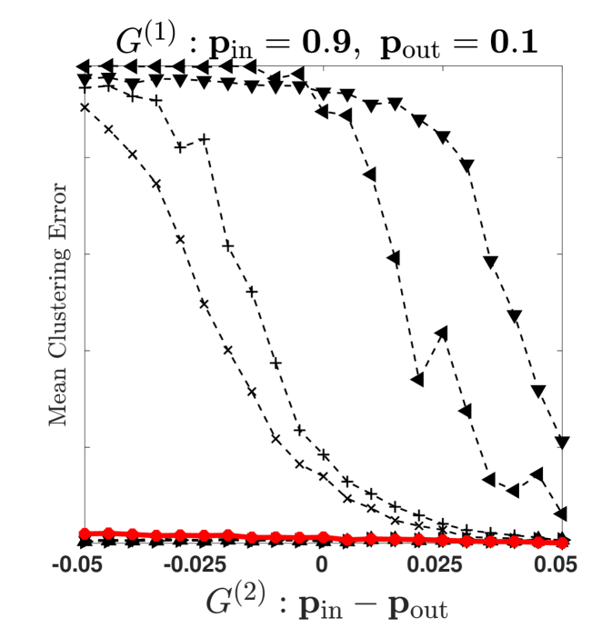
(a) $L_{p}=M_{p}(L_{\textrm{sym}}^{(1)},L_{\textrm{sym}}^{(2)})$

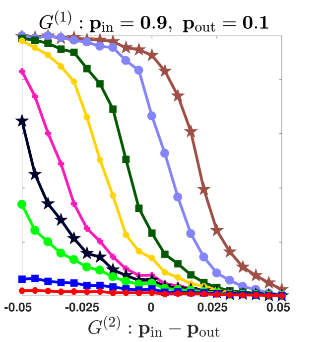
(b) $L_{p}=M_{p}(L_{\textrm{sym}}^{(1)},L_{\textrm{sym}}^{(2)})$

Figure 1: Mean Clustering Error under the SBM with two clusters. First layer $G^{(1)}$ is assortative and ${L_{p}=M_{p}(L_{\textrm{sym}}^{(1)},L_{\textrm{sym}}^{(2)})}$. Second layer $G^{(2)}$ transitions from disassortative to assortative. Fig. 1(a): Comparison of $L_{-10}$ with state of art. Fig. 1(b): Performance of $L_{p}$ with ${p\in\{0,\pm 1,\pm 2,\pm 5,\pm 10\}}$.

The following theorem gives general conditions on the recovery of the ground truth clusters in dependency on $p$ and the size of the shift in $\mathcal{L}_{p}$, see Section 2.2. Note that, in analogy with Lemma 2, as $p\rightarrow-\infty$ the recovery of the ground truth clusters is achieved if at least one of the layers is informative, whereas if $p\rightarrow\infty$ all of them have to be informative in order to recover the ground truth.

   

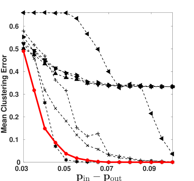
(a)

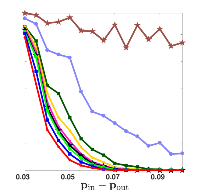
(b)

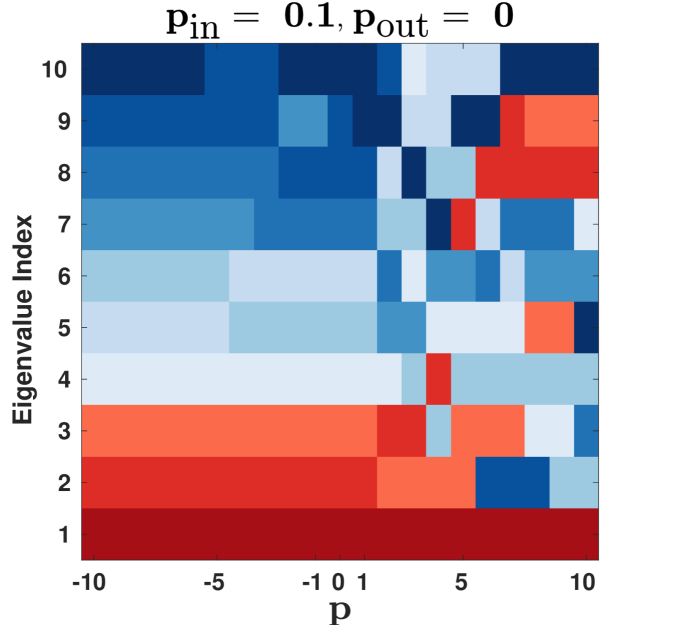
(c)

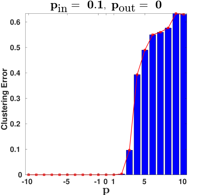
(d)

Figure 2: SBM experiments with three layers. Each layer is informative with respect to one cluster. 2(a): Comparison of $L_{-10}$ with state of art. 2(b): Performance of $L_{p}$ with ${p\in\{0,\pm 1,\pm 2,\pm 5,\pm 10\}}$. 2(c): Eigenvalue ordering of power mean Laplacian $L_{p}$ across different powers. The ordering clearly changes for powers $p\geq 2$, inducing non-informative eigenvectors to the bottom of the spectrum. 2(d): Clustering error of the power mean Laplacian $L_{p}$. Clustering error increases with $p\geq 2$, as suggested by ordering changes depicted in  2(c).

Theorem 1.

Let $p\!\in\![-\infty,\infty]$, then $\bm{\chi}_{1},\ldots,\bm{\chi}_{k}$ correspond to the $k$-smallest eigenvalues of $\mathcal{L}_{p}$ if and only if $m_{p}(\bm{\mu}+\epsilon\mathbf{1})\!<\!1+\epsilon$, where $\bm{\mu}=(1-\rho_{1},\ldots,1-\rho_{T})$, and $\rho_{t}\!=\!(p_{\mathrm{in}}^{(t)}\!-\!p_{\mathrm{out}}^{(t)})/(p_{\mathrm{in}}^{(t)}\!+\!(k\!-\!1)p_{\mathrm{out}}^{(t)})$.

In particular, for $p\to\pm\infty$, we have

1. $\bm{\chi}_{1},\ldots,\bm{\chi}_{k}$ correspond to the $k$-smallest eigenvalues of $\mathcal{L}_{\infty}$ if and only if all layers are informative, i.e. $p_{\mathrm{in}}^{(t)}>p_{\mathrm{out}}^{(t)}$ holds for all $t\in\{1,\ldots,T\}$.

2. $\bm{\chi}_{1},\ldots,\bm{\chi}_{k}$ correspond to the $k$-smallest eigenvalues of $\mathcal{L}_{-\infty}$ if and only if there is at least one informative layer, i.e. there exists a $t\in\{1,\ldots,T\}$ such that $p_{\mathrm{in}}^{(t)}>p_{\mathrm{out}}^{(t)}$.

Theorem 1 shows that the informative eigenvectors of $\mathcal{L}_{p}$ are at the bottom of the spectrum if and only if the scalar power mean of the corresponding eigenvalues is small enough. Since the scalar power mean is monotonically decreasing with respect to $p$, this explains why the limit case $p\to\infty$ is more restrictive than $p\to\!-\infty$. The corollary below shows that the coverage of parameter settings in the SBM for which one recovers the ground truth becomes smaller as $p$ grows.

Corollary 1.

Let $q\leq p$. If $\bm{\chi}_{1},\ldots,\bm{\chi}_{k}$ correspond to the $k$-smallest eigenvalues of $\mathcal{L}_{p}$, then $\bm{\chi}_{1},\ldots,\bm{\chi}_{k}$ correspond to the $k$-smallest eigenvalues of $\mathcal{L}_{q}$.

The previous results hold in expectation. The following experiments show that these findings generalize to the case where one samples from the SBM. In Fig. 1 we present experiments on sparse sampled multilayer graphs from the SBM. We consider two clusters of size $\left|\mathcal{C}\right|=100$ and show the mean of clustering error of $50$ runs. We evaluate the power mean Laplacian $L_{p}$ with $p\in\{0,\pm 1,\pm 2,\pm 5,\pm 10\}$ and compare with other methods described in Section 5.

In Fig. 1 we fix the first layer $G^{(1)}$ to be strongly assortative and let the second layer $G^{(2)}$ run from a disassortative to an assortative configuration. In Fig.1(a) we can see that the power mean Laplacian $L_{-10}$ returns the smallest clustering error, together with the multitensor method, the best single view and the heuristic approach across all parameter settings. The latter two work well by construction in this setting. However, we will see that they fail for the second setting we consider next. All the other competing methods fail as the second graph $G^{(2)}$ becomes non-informative resp. even violates the assumption to be assortative. In Fig. 1(b) we can see that the smaller the value of $p$, the smaller the clustering error of the power mean Laplacian $L_{p}$, as stated in Corollary 1.

3.2 Case 2: No layer contains full information on the clustering structure

We consider a multilayer SBM setting where each individual layer contains only information about one of the clusters and only considering all the layers together reveals the complete cluster structure. For this particular instance, all power mean Laplacians $\mathcal{L}_{p}$ allow to recover the ground truth for any non-zero integer $p$.

For the sake of simplicity, we limit ourselves to the case of three layers and three clusters, showing an assortative behavior in expectation. Let the expected adjacency matrix $\mathcal{W}^{(t)}$ of layer $G^{(t)}$ be defined by

$$\mathcal{W}^{(t)}_{i,j}=\begin{cases}p_{\mathrm{in}},&\quad v_{i},v_{j}\in\mathcal{C}_{t}\text{ or }v_{i},v_{j}\in\overline{\mathcal{C}_{t}}\\ p_{\mathrm{out}},&\quad\textrm{else}\\ \end{cases}$$ (3)

for ${t=1,2,3}$. Note that, up to a node relabeling, the three expected adjacency matrices have the form

$$\underbrace{\left(\begin{array}[]{c|c|c}\pagecolor{black!10}\color[rgb]{0.9,0.9,0.9}1\color[rgb]{0,0,0}&\color[rgb]{1,1,1}1\color[rgb]{0,0,0}&\color[rgb]{1,1,1}1\color[rgb]{0,0,0}\\ \hline\cr\color[rgb]{1,1,1}1\color[rgb]{0,0,0}&\pagecolor{black!10}\color[rgb]{0.9,0.9,0.9}1\color[rgb]{0,0,0}&\pagecolor{black!10}\color[rgb]{0.9,0.9,0.9}1\color[rgb]{0,0,0}\\ \hline\cr\color[rgb]{1,1,1}1\color[rgb]{0,0,0}&\pagecolor{black!10}\color[rgb]{0.9,0.9,0.9}1\color[rgb]{0,0,0}&\pagecolor{black!10}\color[rgb]{0.9,0.9,0.9}1\color[rgb]{0,0,0}\\ \end{array}\right)}_{\mathcal{W}^{(1)}},\quad\underbrace{\left(\begin{array}[]{c|c|c}\pagecolor{black!10}\color[rgb]{0.9,0.9,0.9}1\color[rgb]{0,0,0}&\color[rgb]{1,1,1}1\color[rgb]{0,0,0}&\pagecolor{black!10}\color[rgb]{0.9,0.9,0.9}1\color[rgb]{0,0,0}\\ \hline\cr\color[rgb]{1,1,1}1\color[rgb]{0,0,0}&\pagecolor{black!10}\color[rgb]{0.9,0.9,0.9}1\color[rgb]{0,0,0}&\color[rgb]{1,1,1}1\color[rgb]{0,0,0}\\ \hline\cr\pagecolor{black!10}\color[rgb]{0.9,0.9,0.9}1\color[rgb]{0,0,0}&\color[rgb]{1,1,1}1\color[rgb]{0,0,0}&\pagecolor{black!10}\color[rgb]{0.9,0.9,0.9}1\color[rgb]{0,0,0}\\ \end{array}\right)}_{\mathcal{W}^{(2)}},\quad\underbrace{\left(\begin{array}[]{c|c|c}\pagecolor{black!10}\color[rgb]{0.9,0.9,0.9}1\color[rgb]{0,0,0}&\pagecolor{black!10}\color[rgb]{0.9,0.9,0.9}1\color[rgb]{0,0,0}&\color[rgb]{1,1,1}1\color[rgb]{0,0,0}\\ \hline\cr\pagecolor{black!10}\color[rgb]{0.9,0.9,0.9}1\color[rgb]{0,0,0}&\pagecolor{black!10}\color[rgb]{0.9,0.9,0.9}1\color[rgb]{0,0,0}&\color[rgb]{1,1,1}1\color[rgb]{0,0,0}\\ \hline\cr\color[rgb]{1,1,1}1\color[rgb]{0,0,0}&\color[rgb]{1,1,1}1\color[rgb]{0,0,0}&\pagecolor{black!10}\color[rgb]{0.9,0.9,0.9}1\color[rgb]{0,0,0}\\ \end{array}\right)}_{\mathcal{W}^{(3)}}\,,$$

where each (block) row and column corresponds to a cluster $\mathcal{C}_{i}$ and gray blocks correspond to nodes whose probability of connections is $p_{\mathrm{in}}$, whereas white blocks correspond to nodes whose probability of connections is $p_{\mathrm{out}}$. Let us assume an assortative behavior on all the layers, that is $p_{\mathrm{in}}>p_{\mathrm{out}}$. In this case spectral clustering applied on a single layer ${\mathcal{W}^{(t)}}$ would return cluster $\mathcal{C}_{t}$ and a random partition of the complement, failing to recover the ground truth clustering $\mathcal{C}_{1},\mathcal{C}_{2},\mathcal{C}_{3}$. This is shown in the following Theorem.

Theorem 2.

If $p_{\mathrm{in}}>p_{\mathrm{out}}$, then for any $t=1,2,3$, there exist scalars $\alpha>0$ and $\beta>0$ such that the eigenvectors of $\mathcal{L}_{\mathrm{sym}}^{(t)}$ corresponding to the two smallest eigenvalues are

$$\bm{\chi}_{1}=\alpha\mathbf{1}_{\mathcal{C}_{t}}+\mathbf{1}_{\overline{\mathcal{C}_{t}}}\quad\text{and}\quad\bm{\chi}_{2}=-\beta\mathbf{1}_{\mathcal{C}_{t}}+\mathbf{1}_{\overline{\mathcal{C}_{t}}}$$

whereas any vector orthogonal to both $\bm{\chi}_{1}$ and $\bm{\chi}_{2}$ is an eigenvector for the third smallest eigenvalue.

On the other hand, it turns out that the power mean Laplacian $L_{p}$ is able to merge the information of each layer, obtaining the ground truth clustering, for all integer powers different from zero. This is formally stated in the following.

$\bm{\tilde{p}}$
	0.5	0.6	0.7	0.8	0.9	1.0
$L_{\text{agg}}$	0.3	1.3	3.0	8.0	22.3	100.0
Coreg	0.3	0.0	0.3	0.0	0.0	64.7
BestView	9.7	1.0	0.3	0.0	0.7	77.3
Heuristic	0.0	0.0	0.0	0.0	0.3	59.3
TLMV	0.7	0.7	4.0	6.0	24.7	100.0
RMSC	1.0	1.7	4.0	7.0	19.7	100.0
MT	1.3	0.3	0.7	3.0	17.0	100.0
$L_{10}$	0.0	0.0	0.0	0.0	1.0	100.0
$L_{5}$	0.0	0.0	0.0	0.0	5.0	100.0
$L_{2}$	0.0	0.0	0.3	2.3	18.3	100.0
$L_{1}$	1.0	1.0	3.0	7.0	30.3	100.0
$L_{0}$	4.3	4.3	9.7	15.3	38.3	100.0
$L_{-1}$	6.7	7.7	15.7	16.3	42.3	100.0
$L_{-2}$	8.0	13.0	20.3	20.7	42.7	100.0
$L_{-5}$	22.3	23.0	36.3	37.7	50.0	100.0
$L_{-10}$	69.0	76.3	68.0	67.3	59.7	100.0

$\bm{\mu}$
	0.0	0.1	0.2	0.3	0.4	0.5
$L_{\text{agg}}$	24.7	21.7	21.3	21.7	24.3	21.3
Coreg	16.7	16.7	13.3	11.7	6.0	1.0
BestView	16.7	17.0	17.0	17.7	11.7	9.0
Heuristic	16.7	16.3	15.0	9.0	2.0	0.7
TLMV	25.7	24.3	21.7	23.3	21.0	20.0
RMSC	26.3	22.0	23.0	21.7	20.3	20.0
MT	19.7	19.7	21.0	20.7	20.7	20.7
$L_{10}$	16.7	17.3	17.0	16.7	16.7	16.7
$L_{5}$	17.0	18.0	17.3	17.7	18.0	17.0
$L_{2}$	23.0	21.3	19.3	19.0	20.3	18.0
$L_{1}$	26.3	25.3	24.0	23.0	22.3	21.3
$L_{0}$	33.3	30.3	28.7	28.0	28.0	23.7
$L_{-1}$	36.3	33.0	33.3	32.0	29.0	25.0
$L_{-2}$	37.3	36.3	36.7	34.0	31.3	29.0
$L_{-5}$	48.0	45.0	49.0	44.3	43.0	40.0
$L_{-10}$	71.7	72.3	72.7	74.7	76.3	72.7

Table 1: Percentage of cases where the minimum clustering error is achieved by different methods. Left: Columns correspond to a fixed value of $\tilde{p}$ and we aggregate over $\mu\in\{0.0,0.1,0.2,0.3,0.4,0.5\}$. Left: Columns correspond to a fixed value of $\mu$ and we aggregate over $\tilde{p}\in\{0.5,0.6,0.7,0.8,0.9,1.0\}$.

Theorem 3.

Let $p_{\mathrm{in}}>p_{\mathrm{out}}$ and for $\varepsilon>0$ define

$$\tilde{\mathcal{L}}_{\mathrm{sym}}^{(t)}=\mathcal{L}_{\mathrm{sym}}^{(t)}+\varepsilon I,\quad t=1,2,3.$$

Then the eigenvectors of $\mathcal{L}_{p}=M_{p}(\tilde{\mathcal{L}}_{\mathrm{sym}}^{(1)},\tilde{\mathcal{L}}_{\mathrm{sym}}^{(2)},\tilde{\mathcal{L}}_{\mathrm{sym}}^{(3)})$

corresponding to its three smallest eigenvalues are

$$\bm{\chi}_{1}=\mathbf{1},\quad\bm{\chi}_{2}=\mathbf{1}_{\mathcal{C}_{2}}-\mathbf{1}_{\mathcal{C}_{1}},\quad\text{and}\quad\bm{\chi}_{3}=\mathbf{1}_{\mathcal{C}_{3}}-\mathbf{1}_{\mathcal{C}_{1}}$$

for any nonzero integer $p$.

The proof of Theorem 20 is more delicate than the one of Theorem 1, as it involves the addition of powers of matrices that do not have the same eigenvectors.

Note that Theorem 20 does not distinguish the behavior for distinct values of $p$. In expectation all nonzero integer values of $p$ work the same. This is different to Theorem 1, where the choice of $p$ had a relevant influence on the eigenvector embedding even in expectation. However, we see in the experiments on graphs sampled from the SBM (Figure 2) that the choice of $p$ has indeed a significant influence on the performance even though they are the same in expectation. This suggests that the smaller $p$, the smaller the variance in the difference to the expected behavior in the SBM. We leave this as an open problem if such a dependency can be shown analytically.

In Figs. 2(a) and 2(b) we present the mean clustering error out of ten runs. In Fig. 2(a) one can see that BestView and Heuristic, which rely on clusterings determined by single views, return high clustering errors which correspond to the identification of only a single cluster. The result of Theorem 20 explains this failure. The reason for the increasing clustering error with $p$ can be seen in Fig. 2(c) where we analyze how the ordering of eigenvectors changes for different values of $p$. We can see that for negative powers, the informative eigenvectors belong to the bottom three eigenvalues (denoted in red). For the cases where $p\geq\!2$ the ordering changes, pushing non-informative eigenvectors to the bottom of the spectrum and thus resulting into a high clustering error, as seen in Fig. 2(d). However, we conclude that also for this second case a strongly negative power mean Laplacian as $L_{-10}$ works best.

Input: $\mathbf{x}_{0}$, $p<0$

Output: Eigenpair $(\lambda,\mathbf{x})$ of $M_{p}$

1repeat

2       $\mathbf{u}^{(1)}_{k}$ $\leftarrow$ $(A_{1})^{p}\mathbf{x}_{k}$

3       $\vdots$

4       $\mathbf{u}^{(T)}_{k}$ $\leftarrow$ $(A_{T})^{p}\mathbf{x}_{k}$

5      $\mathbf{y}_{k+1}$ $\leftarrow$ ${\frac{1}{T}}\sum_{{i=1}}^{T}\mathbf{u}^{(i)}_{k}$

6       $\mathbf{x}_{k+1}$ $\leftarrow$ $\mathbf{y}_{k+1}/\|\mathbf{y}_{k+1}\|_{2}$

7      

8until tolerance reached

9$\lambda$ $\leftarrow$ $(\mathbf{x}_{k+1}^{T}\mathbf{x}_{k})^{1/p}$, $\mathbf{x}$ $\leftarrow$ $\mathbf{x}_{k+1}$

Algorithm 2 PM applied to $M_{p}.^{{\color[rgb]{1,1,1}1/2}}$

Input: $\mathbf{u}_{0}=\mathbf{y}$, $V_{0}=[\,\cdot\,],p<0$

Output: $\mathbf{x}=A^{p}\mathbf{y}$

1 $\mathbf{v}_{0}$ $\leftarrow$ $\mathbf{y}/\left|\left|\mathbf{y}\right|\right|_{2}$

2 for $s=0,1,2,\dots,n$ do

3       $\tilde{V}_{s+1}$ $\leftarrow$ $[V_{s},\mathbf{v}_{s}]$

4       $V_{s+1}$ $\leftarrow$ Orthogonalize columns of $\tilde{V}_{s+1}$

5       $H_{s+1}$ $\leftarrow$ $V_{s+1}^{T}AV_{s+1}$

6       $\mathbf{x}_{s+1}$ $\leftarrow$ $V_{s+1}(H_{s+1})^{p}\mathbf{e}_{1}\left|\left|\mathbf{y}\right|\right|_{2}$

7       if tolerance reached then break

8       $\mathbf{v}_{s+1}$ $\leftarrow$ $A\mathbf{v}_{s}$

9      

10 end for

11$\mathbf{x}$ $\leftarrow$ $\mathbf{x}_{s+1}$

Algorithm 3 PKSM for the computation of $A^{p}\mathbf{y}$

[capbesideposition=right,top,capbesidewidth=.6]figure[]

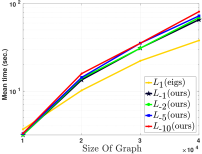
Figure 3: Mean execution time of 10 runs for the power mean Laplacian $L_{p}$. $L_{-1}(\textrm{ours}),L_{-2}(\textrm{ours}),L_{-5}(\textrm{ours}),L_{-10}(\textrm{ours})$ stands for the power mean Laplacian together with our proposed Power Method (Alg. 2) based on the Polynomial Krylov Approximation Method (Alg. 3). $L_{1}(\textrm{eigs})$ stands for the arithmetic mean Laplacian together with Matlab’s eigs function. Experiments are performed using one thread. We generate multilayer graphs with two layers, each with two clusters of same size with parameters $p_{\mathrm{in}}=0.05$ and $p_{\mathrm{in}}=0.025$ and graphs of size $\left|V\right|\in\{10000,20000,30000,40000\}$.

3.3 Case 3: Non-consistent partitions between layers

We now consider the case where all the layers follow the same node partition (as in Section 3.1), but the partitions may fluctuate from layer to layer with a certain probability. We use the multilayer network model introduced in [4]. This generative model considers a graph partition for each layer, allowing the partitions to change from layer to layer according to an interlayer dependency tensor. For the sake of clarity we consider a one-parameter interlayer dependency tensor with parameter $\tilde{p}\in[0,1]$ (i.e. a uniform multiplex network according to the notation used in Section 3.B in [4]), where for $\tilde{p}=0$ the partitions between layers are independent, and for $\tilde{p}=1$ the partitions between layers are identical. Once the partitions are obtained, edges are generated following a multilayer degree-corrected SBM (DCSBM in Section 4 of [4]), according to a one-parameter affinity matrix with parameter $\mu\in[0,1]$, where for $\mu=0$ all edges are within communities whereas for $\mu=1$ edges are assigned ignoring the community structure.

We choose ${\tilde{p}\in\{0.5,0.6,0.7,0.8,0.9,1\}}$ and ${\mu\in\{0.0,0.1,0.2,0.3,0.4,0.5\}}$ and consider all possible combinations of $(\tilde{p},\mu)$. For each pair we count how many times, out of $50$ runs, each method achieves the smallest clustering error. The remaining parameters of the DCSBM are set as follows: exponent $\gamma\!\!=\!\!-3$, minimum degree and maximum degree $k_{min}\!=\!k_{max}\!=\!10$, $\left|V\right|\!=\!100$ nodes, $T\!=\!10$ layers and $K\!=\!2$ communities. As partitions between layers are not necessarily the same, we take the most frequent node assignment among all 10 layers as ground truth clustering.

In Table 1, left side, we show the result for fixed values of $\tilde{p}$ and average over all values of $\mu$. On the right table we show the corresponding results for fixed values of $\mu$ and average over all values of $\tilde{p}$. On the left table we can see that for $\tilde{p}=1$, where the partition is the same in all layers, all methods recover the clustering, while, as one would expect, the performance decreases with smaller values of $\tilde{p}$. Further, we note that the performance of the power mean Laplacian improves as $\tilde{p}$ decreases and $L_{-10}$ again achieves the best result. On the right table we see that performance is degrading with larger values of $\mu$. This is expected as for larger values of $\mu$ the edges inside the clusters are less concentrated. Again the performance of the power mean Laplacian improves as $p$ decreases and $L_{-10}$ performs best.

	3Sources	BBC	BBCS	Wiki	UCI	Citeseer	Cora	WebKB
# vertices	169	685	544	693	2000	3312	2708	187
# layers	3	4	2	2	6	2	2	2
# classes	6	5	5	10	10	6	7	5
$L_{\textrm{agg}}$	0.194	0.156	0.152	0.371	0.162	0.373	0.452	0.277
Coreg	0.215	0.196	0.164	0.784	0.248	0.395	0.659	0.444
Heuristic	0.192	0.218	0.198	0.697	0.280	0.474	0.515	0.400
TLMV	0.284	0.259	0.317	0.412	0.154	0.363	0.533	0.430
RMSC	0.254	0.255	0.194	0.407	0.173	0.422	0.507	0.279
MT	0.249	0.133	0.158	0.544	0.103	0.371	0.436	0.298
$L_{1}$	0.194	0.154	0.148	0.373	0.163	0.285	0.367	0.440
$\bm{L_{-10}}$ (ours)	0.200	0.159	0.144	0.368	0.095	0.283	0.374	0.439

Table 2: Average Clustering Error

4 Computing the smallest eigenvalues and eigenvectors of $M_{p}(A_{1},\dots,A_{T})$

We present an efficient method for the computation of the smallest eigenvalues of $M_{p}(A_{1},\dots,A_{T})$ which does not require the computation of the matrix $M_{p}(A_{1},\dots,A_{T})$. This is particularly important when dealing with large-scale problems as $M_{p}(A_{1},\dots,A_{T})$ is typically dense even though each $A_{i}$ is a sparse matrix. We restrict our attention to the case $p<0$ which is the most interesting one in practice. The positive case $p>0$ as well as the limit case $p\to 0$ deserve a different analysis and are not considered here.

Let $A_{1},\dots,A_{T}$ be positive definite matrices. If ${\lambda_{1}\leq\cdots\leq\lambda_{n}}$ are the eigenvalues of $M_{p}(A_{1},\dots,A_{T})$ corresponding to the eigenvectors $\mathbf{u}_{1},\dots,\mathbf{u}_{n}$, then $\mu_{i}\!=\!(\lambda_{i})^{p}$, $i\!=\!1,\dots,n$, are the eigenvalues of $M_{p}(A_{1},\dots,A_{T})^{p}$ corresponding to the eigenvectors $\mathbf{u}_{i}$. However, the function $f(x)\!=\!x^{p}$ is order reversing for $p<0$. Thus, the relative ordering of the $\mu_{i}$’s changes into $\mu_{1}\geq\cdots\geq\mu_{n}$. Thus, the smallest eigenvalues and eigenvectors of $M_{p}(A_{1},\dots,A_{T})$ can be computed by addressing the largest ones of $M_{p}(A_{1},\dots,A_{T})^{p}$. To this end we propose a power method type outer-scheme, combined with a Krylov subspace approximation inner-method. The pseudo code is presented in Algs. 2 and 3. Each step of the outer iteration in Alg. 2 requires to compute the $p$th power of $T$ matrices times a vector. Computing $A^{p}\times vector$, reduces to the problem of computing the product of a matrix function times a vector. Krylov methods are among the most efficient and most studied strategies to address such a computational issue. As $A^{p}$ is a polynomial in $A$, we apply a Polynomial Krylov Subspace Method (PKSM), whose pseudo code is presented in Alg. 3 and which we briefly describe in the following. For further details we refer to [22] and the references therein. For the sake of generality, below we describe the method for a general positive definite matrix $A$.

The general idea of PKSM $s$-th iteration is to project $A$ onto the subspace $\mathbb{K}^{s}(A,\mathbf{y})=\mathrm{span}\{\mathbf{y},A\mathbf{y},\dots,A^{s-1}\mathbf{y}\}$ and solve the problem there. The projection onto $\mathbb{K}^{s}(A,\mathbf{y})$ is realized by means of the Lanczos process, producing a sequence of matrices $V_{s}$ with orthogonal columns, where the first column of $V_{s}$ is $\mathbf{y}/\left|\left|\mathbf{y}\right|\right|_{2}$ and $\mathrm{range}(V_{s})=\mathbb{K}^{s}(A,\mathbf{y})$. Moreover at each step we have $AV_{s}=V_{s}H_{s}+\mathbf{v}_{s+1}\mathbf{e}_{s}^{T}$ where $H_{s}$ is $s\times s$ symmetric tridiagonal, and $\mathbf{e}_{i}$ is the $i$-th canonical vector. The matrix vector product $\mathbf{x}=A^{p}\mathbf{y}$ is then approximated by $\mathbf{x}_{s}=V_{s}(H_{s})^{p}\mathbf{e}_{1}\|\mathbf{y}\|\approx A^{p}\mathbf{y}$.

Clearly, if operations are done with infinite precision, the exact $\mathbf{x}$ is obtained after $n$ steps. However, in practice, the error $\|\mathbf{x}_{s}-\mathbf{x}\|$ decreases very fast with $s$ and often very few steps are enough to reach a desirable tolerance. Two relevant observations are in order: first, the matrix $H_{s}=V_{s}^{T}AV_{s}$ can be computed iteratively alongside the Lanczos method, thus it does not require any additional matrix multiplication; second, the $p$ power of the matrix $H_{s}$ can be computed directly without any notable increment in the algorithm cost, since $H_{s}$ is tridiagonal of size $s\times s$.

Several eigenvectors can be simultaneously computed with Algs. 2 and 3 by orthonormalizing the current eigenvector approximation at every step of the power method (Alg. 2) (see f.i. algorithm 5.1 Subspace iteration in [46]). Moreover, the outer iteration in Alg. 2 can be easily run in parallel as the vectors $\mathbf{u}_{k}^{(i)}$, $i=1,\dots,T$ can be built independently of each other.

A numerical evaluation of Algs. 2 and 3 is presented in Fig. 3. We consider graphs of sizes ${\left|V\right|\in\{1\!\times\!10^{4},2\!\times\!10^{4},3\!\times\!10^{4},4\!\times\!10^{4}\}}$. Further, for each multilayer graph we generate two assortative graphs with parameters $p_{\mathrm{in}}\!=\!0.05$ and $p_{\mathrm{in}}\!=\!0.025$, following the SBM. Moreover, we consider the power mean Laplacian $L_{p}=M_{p}(L_{\mathrm{sym}}^{(1)},L_{\mathrm{sym}}^{(2)})$ with parameter ${p\!\in\!\{-1,-2,-5,-10\}}$. As a baseline we take the arithmetic mean Laplacian ${L_{1}=M_{1}(L_{\mathrm{sym}}^{(1)},L_{\mathrm{sym}}^{(2)})}$ and use Matlab’s eigs function. For all cases, we compute the two eigenvectors corresponding to the smallest eigenvalues. We present the mean execution time of 10 runs. Experiments are performed using one thread.

5 Experiments

We take the following baseline approaches of spectral clustering applied to: the average adjacency matrix ($\mathbf{L_{agg}}$), the arithmetic mean Laplacian ($\mathbf{L_{1}}$), the layer with the largest spectral gap (Heuristic), and to the layer with the smallest clustering error (BestView). Further, we consider: Pairwise Co-Regularized Spectral Clustering [30], with parameter $\lambda=0.01$ (Coreg), which proposes a spectral embedding generating a clustering consistent among all graph layers, Robust Multi-View Spectral Clustering [58], with parameter $\lambda=0.005$ (RMSC), which obtains a robust consensus representation by fusing noiseless information present among layers, spectral clustering applied to a suitable convex combination of normalized adjacency matrices [66] (TLMV), and a tensor factorization method [11] (MT), which considers a multi-layer mixed membership (SBM).

We take several datasets: 3sources[33], BBC[17] and BBC Sports[18] news articles, a dataset of Wikipedia articles[44], the hand written UCI digits dataset with six different features and citations datasets CiteSeer[34], Cora[36] and WebKB[10], (from WebKB we only take the subset Texas). For each layer we build the corresponding adjacency matrix from the $k$-nearest neighbour graph based on the Pearson linear correlation between nodes, i.e. the higher the correlation the nearer the nodes are. We test all clustering methods over all choices of ${k\in\{20,40,60,80,100\}}$, and present the average clustering error in Table 2. Datasets CiteSeer, Cora and WebKB have two layers: one is a fixed citation network, whereas the second one is the $k$-nearest neighbour graph built on documents features. We can see that in four out of eight datasets the power mean Laplacian $L_{-10}$ gets the smallest clustering error. The largest difference in clustering error is present in the UCI dataset, where the second best is MT. Further, $L_{1}$ presents the smallest clustering error in Cora, being $L_{-10}$ close to it. The smallest clustering error in WebKB is achieved by $L_{\textrm{agg}}$. This dataset is particularly challenging, due to conflictive layers[20].

Acknowledgments. The work of P.M., A.G. and M.H. has been funded by the ERC starting grant NOLEPRO n. 307793. The work of F.T. has been funded by the Marie Curie Individual Fellowship MAGNET n. 744014.

Appendix A Proofs for the Stochastic Block Model analysis

This section has two parts corresponding to the Case 1 and 2 of the stochastic block model analysis. At the beginning of each of these sections, we first state what will be proved and discuss further refinements implied by the results presented here. For convenience we recall the notation where needed.

The correspondence between the results of the main paper and those proved here is as follows: In Section A.1 we discuss and prove Lemma 1, 2, Theorem 1 and Corollary 1 of the main paper. These results are directly implied by Lemma 3, Theorem 4 and Corollaries 2, 3, respectively, of the present manuscript. Then, in Section A.2, we prove Theorem 2 and Theorem 3 of the main paper which are respectively equivalent to Theorems 5 and 6 below.

Before proceeding to the proofs, let us recall the setting. Let $V=\{v_{1},\ldots,v_{n}\}$ be a set of nodes and let $T$ be the number of layers, represented by the adjacency matrices $\mathbb{W}=\{W^{(1)},\ldots,W^{(T)}\}$. For each matrix $W^{(t)}$ we have a graph $G^{(t)}=(V,W^{(t)})$ and, overall, a multilayer graph ${\mathbb{G}=(G^{(1)},\ldots,G^{(T)})}$. We denote the ground truth clusters by $\mathcal{C}_{1},\ldots,\mathcal{C}_{k}$ and assume that they all have the same size, i.e. $\left|\mathcal{C}_{i}\right|=\left|\mathcal{C}\right|$ for $i=1,\ldots,k$.

In the following, we denote the identity matrix in $\mathbb{R}^{m}$ by $I_{m}$. Furthermore, for a matrix $X\in\mathbb{R}^{m\times m}$, we denote its eigenvalues by $\lambda_{1}(X),\ldots,\lambda_{m}(X)$.

A.1 All layers have the same clustering structure

For $t=1,\ldots,T$, let $p_{\mathrm{in}}^{(t)}$ (resp. $p_{\mathrm{out}}^{(t)}$) denote the probability that there exists an edge in layer $G^{(t)}$ between nodes that belong to the same (resp. different) clusters. Suppose that for $t=1,\ldots,T$, the expected adjacency matrix $\mathcal{W}^{(t)}\in\mathbb{R}^{n\times n}$ of $G^{(t)}$ is given for $i,j=1,\ldots,n$ as

$$\mathcal{W}^{(t)}_{ij}=\begin{cases}p_{\mathrm{in}}^{(t)}&\text{if }v_{i},v_{j}\text{ belong to the same cluster}\\ p_{\mathrm{out}}^{(t)}&\text{otherwise}.\end{cases}$$

Furthermore, for every $t=1,\ldots,T,$ and $\epsilon\geq 0$, let

$$\mathcal{D}^{(t)}=\mathrm{diag}(\mathcal{W}^{(t)}\mathbf{1}),\quad\rho_{t}=\frac{p_{\mathrm{in}}^{(t)}-p_{\mathrm{out}}^{(t)}}{p_{\mathrm{in}}^{(t)}+(k-1)p_{\mathrm{out}}^{(t)}},$$

$$L_{sym}^{(t)}=I_{n}-(\mathcal{D}^{(t)})^{-1/2}\mathcal{W}^{(t)}(\mathcal{D}^{(t)})^{-1/2}+\epsilon I_{n}$$

Observe that $L_{sym}^{(t)}$ is the normalized Laplacian of the expected graph plus a diagonal shift. The diagonal shift is necessary to enforce this matrix to be positive definite for the cases $p\leq 0$, as stated in [5].

We consider the vectors $\bm{\chi}_{1},\ldots,\bm{\chi}_{k}\in\mathbb{R}^{n}$ defined as

$$\bm{\chi}_{1}=\mathbf{1},\quad\bm{\chi}_{i}=(k-1)\mathbf{1}_{\mathcal{C}_{i}}-\mathbf{1}_{\overline{\mathcal{C}_{i}}},\quad i=2,\ldots,k.$$

By construction, $\bm{\chi}_{1},\ldots,\bm{\chi}_{k}$ are all eigenvectors of $\mathcal{W}^{(t)}$ for every $t=1,\ldots,T$. These eigenvectors are precisely the vectors allowing to recover the ground truth clusters. Let

$$\mathcal{L}_{p}=M_{p}\big{(}L_{sym}^{(1)},\ldots,L_{sym}^{(T)}\big{)}$$

where we assume that $\epsilon>0$ if $p\leq 0$. We prove the following:

Theorem 4.

Let $p\in[-\infty,\infty]$, and assume that $\epsilon>0$ if $p\leq 0$. Then, there exists $\lambda_{i}$ such that $\mathcal{L}_{p}\bm{\chi}_{i}=\lambda_{i}\bm{\chi}_{i}$ for all $i=1,\ldots,k$. Furthermore, $\lambda_{1},\ldots,\lambda_{k}$ are the $k$-smallest eigenvalues of $\mathcal{L}_{p}$ if and only if $m_{p}(\bm{\mu}+\epsilon\mathbf{1})<1+\epsilon$, where $\bm{\mu}=(1-\rho_{1},\ldots,1-\rho_{T})$.

Before giving a proof of Theorem 4 we discuss some of its implications in order to motivate the result. First, we note that it implies that if $\bm{\chi}_{1},\ldots,\bm{\chi}_{k}$ are among the smallest eigenvectors of $\mathcal{L}_{p}$ then they are among the smallest eigenvectors of $\mathcal{L}_{q}$ for any $q\leq p$.

Corollary 2.

Let $q\leq p$ and assume that $\epsilon>0$ if $\min\{p,q\}\leq 0$. If $\bm{\chi}_{1},\ldots,\bm{\chi}_{k}$ correspond to the $k$-smallest eigenvalues of $\mathcal{L}_{p}$, then $\bm{\chi}_{1},\ldots,\bm{\chi}_{k}$ correspond to the $k$-smallest eigenvalues of $\mathcal{L}_{q}$.

Proof.

If $\lambda_{1},\ldots,\lambda_{k}$ are among the $k$-smallest eigenvalues of $\mathcal{L}_{p}$, then by Theorem 4, we have $m_{p}(\bm{\mu}+\epsilon\mathbf{1})<1+\epsilon$. As $m_{q}(\bm{\mu}+\epsilon\mathbf{1})\leq m_{p}(\bm{\mu}+\epsilon\mathbf{1})$, Theorem 4 concludes the proof. ∎

The next corollary deals with the extreme cases where $p=\pm\infty$. In particular, it implies that whenever at least one layer $G^{(t)}$ is informative then the eigenvectors of $\mathcal{L}_{-\infty}$ allow to recover the clusters. This contrasts with $p=\infty$ where the clusters can be recovered from the eigenvectors of $\mathcal{L}_{\infty}$ if and only if all layers are informative.

Corollary 3.

Let $p\in[-\infty,\infty]$ and $\epsilon>0$ if $p\leq 0$.

1. If $p=\infty$, then $\bm{\chi}_{1},\ldots,\bm{\chi}_{k}$ correspond to the $k$-smallest eigenvalues of $\mathcal{L}_{\infty}$ if and only if all layers are informative, i.e. $p_{\mathrm{in}}^{(t)}>p_{\mathrm{out}}^{(t)}$ holds for all $t\in\{1,\ldots,T\}$.

2. If $p=-\infty$, then $\bm{\chi}_{1},\ldots,\bm{\chi}_{k}$ correspond to the $k$-smallest eigenvalues of $\mathcal{L}_{-\infty}$ if and only if there is at least one informative layer, i.e. there exists a $t\in\{1,\ldots,T\}$ such that $p_{\mathrm{in}}^{(t)}>p_{\mathrm{out}}^{(t)}$.

Proof.

Recall that $\lim_{p\to\infty}m_{p}(\mathbf{v})=\max_{i=1,\ldots,m}v_{i}$ and $\lim_{p\to-\infty}m_{p}(\mathbf{v})=\min_{i=1,\ldots,m}v_{i}$ for any $\mathbf{v}\in\mathbb{R}^{m}$ with nonnegative entries. Hence, we have $m_{\pm\infty}(\bm{\mu}+\epsilon\mathbf{1})=m_{\pm\infty}(\bm{\mu})+\epsilon$ and thus the condition $m_{p}(\bm{\mu}+\epsilon\mathbf{1})<1+\epsilon$ of Theorem 4 reduces to $m_{\pm\infty}(\bm{\mu})<1$ for $p=\pm\infty$. Furthermore, note that we have $\mu_{t}=1-\rho_{t}<1$ if and only if $p_{\mathrm{in}}^{(t)}>p_{\mathrm{out}}^{(t)}$. To conclude, note that $m_{\infty}(\bm{\mu})=\max_{t=1,\ldots,T}\mu_{t}<1$ if and only if $\mu_{t}<1$ for all $t=1,\ldots,T$ and $m_{-\infty}(\bm{\mu})=\min_{t=1,\ldots,T}\mu_{t}<1$ if and only if there exists $t\in\{1,\ldots,T\}$ such that $\mu_{t}<1$. ∎

For the proof of Theorem 4, we give an explicit formula for eigenvalues of $\mathcal{L}_{p}$ in terms of the eigenvalues of $L_{sym}^{(1)},\ldots,L_{sym}^{(T)}$. Then, we discuss the ordering of these eigenvalues. Furthermore, we show that $\bm{\chi}_{i}$ are all eigenvectors of $\mathcal{L}_{p}$ and compute their corresponding eigenvalues.

By construction, there are $k$ eigenvectors $\bm{\chi}_{i}$ of $\mathcal{W}^{(t)}$ corresponding to a possibly nonzero eigenvalue $\lambda_{i}^{(t)}$. These are given by

$$\bm{\chi}_{1}=\mathbf{1},\qquad\lambda_{1}^{(t)}=\left|\mathcal{C}\right|(p_{\mathrm{in}}^{(t)}+(k-1)p_{\mathrm{out}}^{(t)}),$$

$$\bm{\chi}_{i}=(k-1)\mathbf{1}_{\mathcal{C}_{i}}-\mathbf{1}_{\overline{\mathcal{C}_{i}}},\quad\lambda_{i}^{(t)}=\left|\mathcal{C}\right|(p_{\mathrm{in}}^{(t)}-p_{\mathrm{out}}^{(t)})$$

for $i=2,\ldots,k$. It follows that $\bm{\chi}_{1},\ldots,\bm{\chi}_{k}$ are eigenvectors of $L_{sym}^{(t)}$ with eigenvalues $\lambda_{i}(L_{sym}^{(t)})$. Furthermore, we have

$$\lambda_{1}(L_{sym}^{(t)})={\color[rgb]{0,0,0}\epsilon},\quad\lambda_{i}(L_{sym}^{(t)})=1-\rho_{t}{\color[rgb]{0,0,0}+\epsilon},\quad i=2,\ldots,k,$$

$$\lambda_{j}(L_{sym}^{(t)})=1{\color[rgb]{0,0,0}+\epsilon},\quad j=k+1,\ldots,n$$ (4)

Let

$$\mathcal{L}_{p}=M_{p}\big{(}L_{sym}^{(1)},\ldots,L_{sym}^{(T)}\big{)}.$$

The following lemma will be helpful to show that $\bm{\chi}_{1},\ldots,\bm{\chi}_{k}$ are all eigenvectors $\mathcal{L}_{p}$ and gives a formula for their corresponding eigenvalue.

Lemma 3.

Let $A_{1},\ldots,A_{T}\in\mathbb{R}^{n\times n}$ be symmetric positive semi-definite matrices and let $p\in\mathbb{R}$. Suppose that $A_{1},\ldots,A_{T}$ are positive definite if $p\leq 0$. If $\mathbf{u}$ is an eigenvector of $A_{i}$ with corresponding eigenvalue $\lambda_{i}$ for all $i=1,\ldots,T$, then $\mathbf{u}$ is an eigenvector of $M_{p}(A_{1},\ldots,A_{T})$ with eigenvalue $m_{p}(\lambda_{1},\ldots,\lambda_{T})$.

Proof.

First, note that $M=M_{p}(A_{1},\ldots,A_{T})$ is symmetric positive (semi-)definite as it is a positive sum of such matrices. In particular, $M$ is diagonalizable and thus the eigenvectors of $M$ and $M^{p}$ are the same for every $p$. Now, as $A_{i}\mathbf{u}=\lambda_{i}\mathbf{u}$ for $i=1,\ldots,T$, we have $A_{i}^{p}\mathbf{u}=\lambda_{i}^{p}\mathbf{u}$ for all $i$ and thus

$$M_{p}^{p}(A_{1},\ldots,A_{T})\mathbf{u} ={\frac{1}{T}}\sum_{{i=1}}^{T}A_{i}^{p}\mathbf{u}={\frac{1}{T}}\sum_{{i=1}}^{T}\lambda_{i}^{p}\mathbf{u}$$

$$=m_{p}^{p}(\lambda_{1},\ldots,\lambda_{T})\mathbf{u}.$$

Thus, $\mathbf{u}$ is an eigenvector of $M_{p}(A_{1},\ldots,A_{T})$ with eigenvalue $m_{p}(\lambda_{1},\ldots,\lambda_{T})$. ∎

The above lemma, allows to obtain an explicit formula for $\mathcal{L}_{p}$ which fully describes its spectrum. Indeed, we have the following

Corollary 4.

Let $X$ and $\Lambda^{(1)}$ be matrices such that $L_{sym}^{(1)}=X\Lambda^{(1)}X^{T}$, $X$ is orthogonal and $\Lambda^{(1)}=\mathrm{diag}(\lambda_{1}(L_{sym}^{(1)}),\ldots,\lambda_{n}(L_{sym}^{(1)}))$. Then, we have $\mathcal{L}_{p}=X\Lambda X$ where $\Lambda$ is the diagonal matrix $\Lambda=\mathrm{diag}(\lambda_{1}(\mathcal{L}_{p}),\ldots,\lambda_{n}(\mathcal{L}_{p}))$ with $\lambda_{i}(\mathcal{L}_{p})=m_{p}(\lambda_{i}(L_{sym}^{(1)}),\ldots,\lambda_{i}(L_{sym}^{(T)}))$, for all $i=1,\ldots,n$.

Proof.

As $L_{sym}^{(t)}$ have the same eigenvectors for every $t=1,\ldots,T$, it follows by Lemma 3 that $\mathcal{L}_{p}X=X\Lambda$ and thus $\mathcal{L}_{p}=X\Lambda X^{\top}$. ∎

We note that on top of providing information on the spectral properties of $\mathcal{L}_{p}$, Corollary 4 ensures the existence of $\mathcal{L}_{\pm\infty}\in\mathbb{R}^{n\times n}$ such that $\lim_{p\to\pm\infty}\mathcal{L}_{p}=\mathcal{L}_{\pm\infty}$.

Combining Lemma 3 with equation (A.1) we obtain the following

Lemma 4.

The limits $\lim_{p\to\pm\infty}\mathcal{L}_{p}=\mathcal{L}_{\pm\infty}$ exist. Furthermore, for $p\in[-\infty,\infty]$, we have $\mathcal{L}_{p}\bm{\chi}_{i}=\lambda_{i}\bm{\chi}_{i}$ with

$$\lambda_{1}=\epsilon,\quad\lambda_{i}=m_{p}(\bm{\mu}+\epsilon\mathbf{1}),\quad i=2,\ldots,k$$

where $\bm{\mu}=(1-\rho_{1},\ldots,1-\rho_{T})$. Furthermore, the remaining eigenvalues satisfy $\lambda_{k+1}=\cdots=\lambda_{n}=1+\epsilon$.

Proof.

With Corollary 4 and Equation (A.1) we directly obtain for $i=2,\ldots,k$ and $j=k+1,\ldots,n$,

$$\lambda_{1} =\Big{(}\frac{1}{T}\sum_{t=1}^{T}\epsilon^{p}\Big{)}^{1/p}=m_{p}(\epsilon\mathbf{1})=\epsilon$$

$$\lambda_{i} =\Big{(}\frac{1}{T}\sum_{t=1}^{T}(1-\rho_{t}+\epsilon)^{p}\Big{)}^{1/p}=m_{p}(\bm{\mu}+\epsilon\mathbf{1})$$

$$\lambda_{j} =\Big{(}\frac{1}{T}\sum_{t=1}^{T}(1+\epsilon)^{p}\Big{)}^{1/p}=m_{p}((1+\epsilon)\mathbf{1})=1+\epsilon$$

∎

We are now ready to prove Theorem 4.

Proof of Theorem 4.

Clearly, $\lambda_{1},\ldots,\lambda_{k}$ are among the $k$-smallest eigenvalues of $\mathcal{L}_{p}$ if and only if $\lambda_{1}<\lambda_{k+1}\leq\cdots\leq\lambda_{n}$ and $\lambda_{2}\leq\ldots\leq\lambda_{k}<\lambda_{k+1}\leq\cdots\lambda_{n}$ where $\lambda_{1},\ldots,\lambda_{n}$ are all eigenvalues of $\mathcal{L}_{p}$. By Lemma 4, we have $\lambda_{1}=\epsilon$, $\lambda_{2}=\cdots=\lambda_{k}=m_{p}(\bm{\mu}+\epsilon\mathbf{1})$ and $\lambda_{k+1}=\cdots=\lambda_{n}=1+\epsilon$. Clearly $\lambda_{1}=\epsilon<1+\epsilon=\lambda_{k}\leq\cdots\leq\lambda_{n}$, thus, the first condition holds. Hence, $\lambda_{1},\ldots,\lambda_{k}$ correspond to the $k$-smallest eigenvalues of $\mathcal{L}_{p}$ if and only if $m_{p}(\bm{\mu}+\epsilon\mathbf{1})<1+\epsilon$ which concludes the proof. ∎

A.2 No layer contains full information of the Graph

In this setting, we fix the number $k$ of cluster to $k=3$.

For convenience, we slightly overload the notation for the remaining of this section: we denote by $n$ the size of each cluster $\mathcal{C}_{1},\dots,\mathcal{C}_{k}$, i.e. $\left|\mathcal{C}_{i}\right|=\left|\mathcal{C}\right|=n$ for $i=1,\dots,k$. Thus, the size of the graph is expressed in terms of the number and size of clusters, i.e. $\left|V\right|=nk$.

Furthermore, we suppose that for $t=1,2,3$, the expected adjacency matrix $\mathcal{W}^{(t)}\in\mathbb{R}^{3n\times 3n}$ of $G^{(t)}$, are given, for all $i,j=1,\ldots,3n$, as

$$\mathcal{W}^{(t)}_{ij}=\begin{cases}p_{in}&\text{if }v_{i},v_{j}\in\mathcal{C}_{t}\text{ or }v_{i},v_{j}\in\overline{\mathcal{C}_{t}}\\ p_{out}&\text{otherwise},\end{cases}$$

where $0<p_{out}\leq p_{in}\leq 1$. For $t=1,2,3$ and $\epsilon\geq 0$, let $\mathcal{D}^{(t)}=\mathrm{diag}(\mathcal{W}^{(t)}\mathbf{1})$,

$$L_{sym}^{(t)}=I-(\mathcal{D}^{(t)})^{-1/2}\mathcal{W}^{(t)}(\mathcal{D}^{(t)})^{-1/2}+\epsilon I,$$

and for a nonzero integer $p$ let

$$\mathcal{L}_{p}=M_{p}(L_{sym}^{(1)},L_{sym}^{(2)},L_{sym}^{(3)}),$$

where we assume that $\epsilon>0$ if $p<0$. Consider further $\bm{\chi}_{1},\bm{\chi}_{2},\bm{\chi}_{3}\in\mathbb{R}^{3n}$ the vectors defined as

$$\bm{\chi}_{1}=\mathbf{1},\quad\bm{\chi}_{2}=\mathbf{1}_{\mathcal{C}_{1}}-\mathbf{1}_{\mathcal{C}_{2}},\quad\bm{\chi}_{3}=\mathbf{1}_{\mathcal{C}_{1}}-\mathbf{1}_{\mathcal{C}_{3}}.$$

In opposition to the previous model, it turns out that $L_{sym}^{(1)},L_{sym}^{(2)}$ and $L_{sym}^{(3)}$ do not commute and thus do not share the same eigenvectors. Hence, we can not derive an explicit expression for $\mathcal{L}_{p}$ as in Corollary 4. In particular this implies that we need to use different mathematical tools in order to study the eigenpairs of $\mathcal{L}_{p}$.

The first main result of this section, presented in Theorem 5, shows that, in general, the ground truth clusters can not be reconstructed from the $3$ smallest eigenvectors of $L_{sym}^{(t)}$ for any $t=1,2,3$.

Theorem 5.

If $1\geq p_{\mathrm{in}}>p_{\mathrm{out}}>0$, then for any $t=1,2,3$, there exist scalars $\alpha>0$ and $\beta>0$ such that the eigenvectors of $\mathcal{L}_{\mathrm{sym}}^{(t)}$ corresponding to the two smallest eigenvalues are

$$\bm{\varkappa}_{1}=\alpha\mathbf{1}_{\mathcal{C}_{t}}+\mathbf{1}_{\overline{\mathcal{C}_{t}}}\quad\text{and}\quad\bm{\varkappa}_{2}=-\beta\mathbf{1}_{\mathcal{C}_{t}}+\mathbf{1}_{\overline{\mathcal{C}_{t}}}$$

whereas any vector orthogonal to both $\bm{\varkappa}_{1}$ and $\bm{\varkappa}_{2}$ is an eigenvector for the third smallest eigenvalue.

In fact, we prove even more by giving a full description of the eigenvectors of $L_{sym}^{(t)}$ as well as the ordering of their corresponding eigenvalues. These results can be found in Lemma 14 below.

Our second main result is the following Theorem 6. It shows that the ground truth clusters can always be recovered from the three smallest eigenvectors of $\mathcal{L}_{p}$.

Theorem 6.

Let $p$ be any nonzero integer and assume that $\epsilon>0$ if $p<0$. Furthermore, suppose that $0<p_{out}<p_{in}\leq 1$. Then, there exists $\lambda_{i}$ such that $\mathcal{L}_{p}\bm{\chi}_{i}=\lambda_{i}\bm{\chi}_{i}$ for $i=1,2,3$ and $\lambda_{1},\lambda_{2},\lambda_{3}$ are the three smallest eigenvalues of $\mathcal{L}_{p}$.

Again, we actually prove more than just Theorem 6. In fact, a full description of the eigenvectors of $\mathcal{L}_{p}$ and of the ordering of their corresponding eigenvalues is given in Lemma 20 below.

For the proof of Theorems 5 and 6, and the corresponding additional results, we proceed as follows. First we assume that $n=|\mathcal{C}_{i}|=1$ and prove our claims. Then, we generalize these results to the case $n>1$. For the sake of clarity, as we will need to refer to the case $n=1$ for the proofs of the case $n>1$, we put a tilde on the matrices in $\mathbb{R}^{3\times 3}$.

The case $n=1$:

Suppose that $n=1$, then $\tilde{\mathcal{L}}_{\mathrm{sym}}=L_{sym}^{(1)}$ is given by

$$\tilde{\mathcal{L}}_{\mathrm{sym}}=\tau I_{3}-\tilde{\mathcal{D}}^{-1/2}\tilde{\mathcal{W}}\tilde{\mathcal{D}}^{-1/2}=\tau I_{3}-\tilde{\mathcal{M}},$$

where $\tau=1+\epsilon$, $\tilde{\mathcal{W}}=\mathcal{W}^{(1)}$, $\tilde{\mathcal{D}}=\mathrm{diag}(\tilde{\mathcal{W}}\mathbf{1})$,

$$\tilde{\mathcal{D}}=\begin{pmatrix}\alpha&0&0\\ 0&\beta&0\\ 0&0&\beta\end{pmatrix},\qquad\tilde{\mathcal{M}}=\begin{pmatrix}a&b&b\\ b&c&c\\ b&c&c\end{pmatrix},$$ (5)

and $\alpha,\beta,a,b,c>0$ are given by

$$\alpha=p_{in}+2p_{out},\qquad\beta=2p_{in}+p_{out},$$

$$a=\frac{p_{in}}{\alpha},\qquad b=\frac{p_{out}}{\sqrt{\alpha\beta}},\qquad c=\frac{p_{in}}{\beta}.$$

Moreover, note that for any $(\lambda,\mathbf{v})\in\mathbb{R}\times\mathbb{R}^{3}$ we have

$$\tilde{\mathcal{M}}\mathbf{v}=\lambda\mathbf{v}\qquad\iff\qquad\tilde{\mathcal{L}}_{\mathrm{sym}}\mathbf{v}=(\tau-\lambda)\mathbf{v}.$$ (6)

This implies that we can study the spectrum of $\tilde{\mathcal{M}}$ in order to obtain the spectrum of $\tilde{\mathcal{L}}_{\mathrm{sym}}$. We have the following lemma:

Lemma 5.

Suppose that $p_{out}>0$ and let $\Delta>0$ be defined as $\Delta=\sqrt{(a-2c)^{2}+8b^{2}}$. Then the eigenvalues of $\tilde{\mathcal{M}}$ are

$$\tilde{\lambda}_{1}=0,\qquad\tilde{\lambda}_{2}=\frac{a+2c-\Delta}{2},\qquad\tilde{\lambda}_{3}=1,$$

and it holds $\tilde{\lambda}_{1}<\tilde{\lambda}_{2}<\tilde{\lambda}_{3}$. Furthermore, the corresponding eigenvectors are given by

$$\mathbf{u}_{1}=(0,-1,1)^{\top},\qquad\mathbf{u}_{2}=\Big{(}\frac{a-2c-\Delta}{2b},1,1\Big{)}^{\top},$$

$$\mathbf{u}_{3}=\big{(}\sqrt{\alpha},\sqrt{\beta},\sqrt{\beta}\big{)}^{\top},$$

and it holds $\frac{a-2c-\Delta}{2b}<0$.

Proof.

The equality $\tilde{\mathcal{M}}\mathbf{u}_{1}=0$ follows from a direct computation. Furthermore, note that $\mathbf{u}_{3}=\tilde{\mathcal{D}}^{1/2}\mathbf{1}$ and so

$$\tilde{\mathcal{M}}\mathbf{u}_{3} =\tilde{\mathcal{D}}^{-1/2}\tilde{\mathcal{W}}\tilde{\mathcal{D}}^{-1/2}\mathcal{D}^{1/2}\mathbf{1}=\tilde{\mathcal{D}}^{-1/2}\tilde{\mathcal{W}}\mathbf{1}=\mathbf{u}_{3}$$

implying $\tilde{\mathcal{M}}\mathbf{u}_{3}=\mathbf{u}_{3}$. Now, let $s_{\pm}=\frac{a-2c\pm\Delta}{2b}$. Then $s_{+}$ and $s_{-}$ are the solutions of the quadratic equation $bs^{2}+(2c-a)s-2b=0$ which can be rearranged as $as+2b=(bs+2c)s.$ The latter equation is equivalent to

$$\begin{cases}as+2b=\lambda s\\ bs+2c=\lambda\end{cases}\quad\iff\quad\tilde{\mathcal{M}}\begin{pmatrix}s\\ 1\\ 1\end{pmatrix}=\lambda\begin{pmatrix}s\\ 1\\ 1\end{pmatrix}.$$

Hence, $\mathbf{u}_{\pm}=(s_{\pm},1,1)$ are both eigenvectors of $\tilde{\mathcal{M}}$ corresponding to the eigenvalues

$$\lambda_{\pm}=b\,s_{\pm}+2c=\frac{a-2c\pm\Delta}{2}+2c=\frac{a+2c\pm\Delta}{2}.$$

Note in particular that we have $\mathbf{u}_{2}=\mathbf{u}_{-}$ and $\tilde{\lambda}_{2}=\lambda_{-}$. This concludes the proof that $(\lambda_{i},\mathbf{u}_{i})$ are eigenpairs of $\tilde{\mathcal{M}}$ for $i=1,2,3$. We now show that $\tilde{\lambda}_{1}<\tilde{\lambda}_{2}<\tilde{\lambda}_{3}$ and $(a-2c-\Delta)/2b<0$.

As $\Delta>0$, we have $\lambda_{-}<\lambda_{+}$. We prove $\lambda_{-}>0$. As $p_{in}>p_{out}$ by assumption, the definition of $a,b,c>0$ implies that

$$b^{2} =\frac{p_{out}^{2}}{(2p_{in}+p_{out})(p_{in}+2p_{out})}$$

$$<\frac{p_{in}^{2}}{(2p_{in}+p_{out})(p_{in}+2p_{out})}=ac.$$

And from $ac>b^{2}$ it follows that $a^{2}+4ac+4c^{2}>a^{2}-4ac+4c^{2}+8b^{2}$ which implies that $(a+2c)^{2}>(a-2c)^{2}+8b^{2}=\Delta^{2}.$ Hence, $a+2c-\Delta>0$ and thus $\lambda_{-}>0$. Thus we have $0<\lambda_{-}<\lambda_{+}$. Now, as $\tilde{\mathcal{M}}$ has strictly positive entries, the Perron-Frobenius theorem (see for instance Theorem 1.1 in [56]) implies that $\tilde{\mathcal{M}}$ has a unique nonnegative eigenvector $\mathbf{u}$. Furthermore, $\mathbf{u}$ has positive entries and its corresponding eigenvalue is the spectral radius of $\tilde{\mathcal{M}}$. As $\mathbf{u}_{3}=\tilde{\mathcal{D}}^{1/2}\mathbf{1}$ has positive entries and is an eigenvector of $\tilde{\mathcal{M}}$, we have $\mathbf{u}=\mathbf{u}_{3}$. It follows that $\rho(\tilde{\mathcal{M}})=\lambda_{+}=\tilde{\lambda}_{3}$. Furthermore, $\mathbf{u}_{2}$ must have a strictly negative entry and thus it holds $s_{-}<0$. ∎

Combining the results of Lemma 5 and Equation (6) we directly obtain the following corollary which fully describes the eigenvectors of $\tilde{\mathcal{L}}_{\mathrm{sym}}$ as well as the ordering of the corresponding eigenvalues:

Corollary 5.

There exists $\tilde{\lambda}\in(0,1)$ and $s_{-}<0<s_{+}<1$ such that $\big{(}\tau-1,(s_{+},1,1)^{\top}\big{)},\big{(}\tau-\tilde{\lambda},(s_{-},1,1)^{\top}\big{)},\big{(}\tau,(0,-1,1)^{\top}\big{)}$ are the eigenpairs of $\tilde{\mathcal{L}}_{\mathrm{sym}}$.

Proof.

The only thing which is not directly implied by Lemma 5 and Equation (6) is that $s_{+}<1$. But this follows again from Lemma 5. Indeed, as $(s_{+},1,1)$ and $(\sqrt{\alpha},\sqrt{\beta},\sqrt{\beta})$ must span the same line, we have

$$s_{+}=\sqrt{\frac{\alpha}{\beta}}=\sqrt{\frac{p_{in}+2p_{out}}{2p_{in}+p_{out}}}.$$

As $p_{out}<p_{in}$, we get $0<s_{+}<1$. ∎

Now, we study the spectral properties of $\mathcal{\tilde{L}}_{p}=\mathcal{L}_{p}\in\mathbb{R}^{3\times 3}$. To this end, for $t=1,2,3$ let $\tilde{\mathcal{W}}^{(t)}={\mathcal{W}^{(t)}},\tilde{\mathcal{L}}_{\operatorname{sym}}^{(t)}=L_{sym}^{(t)}\in\mathbb{R}^{3\times 3}$. Furthermore, consider the permutation matrices $\tilde{P}_{1},\tilde{P}_{2},\tilde{P}_{3}\in\mathbb{R}^{3\times 3}$ defined as

$$\tilde{P}_{1}=I_{3},\quad\tilde{P}_{2}=\begin{pmatrix}0&0&1\\ 0&1&0\\ 1&0&0\end{pmatrix},\quad\tilde{P}_{3}=\begin{pmatrix}0&1&0\\ 1&0&0\\ 0&0&1\end{pmatrix}.$$

Then, we have $\tilde{\mathcal{W}}^{(t)}=\tilde{P}_{t}\tilde{\mathcal{W}}\tilde{P}_{t}$ for $t=1,2,3$. The following lemma relates $\tilde{\mathcal{L}}_{\operatorname{sym}}^{(t)}$ and $\tilde{\mathcal{L}}_{\mathrm{sym}}$.

Lemma 6.

For $t=1,2,3$, we have $\tilde{P}_{t}=\tilde{P}_{t}^{-1}=\tilde{P}_{t}^{\top}$ and $\tilde{\mathcal{L}}_{\operatorname{sym}}^{(t)}=\tilde{P}_{t}\tilde{\mathcal{L}}_{\mathrm{sym}}\tilde{P}_{t}$.

Proof.

The identity $\tilde{P}_{t}=\tilde{P}_{t}^{-1}=\tilde{P}_{t}^{\top}$ follows by a direct computation. Now, as $\tilde{P}_{t}\mathbf{1}=\mathbf{1}$, we have $\tilde{P}_{t}\tilde{\mathcal{W}}\tilde{P}_{t}\mathbf{1}=\tilde{P}_{t}\tilde{\mathcal{W}}\mathbf{1}$. Assuming the exponents on the vector in the following expressions are taken component wise, we have $\mathrm{diag}(\tilde{\mathcal{W}}\mathbf{1})^{-1/2}=\mathrm{diag}\big{(}(\tilde{\mathcal{W}}\mathbf{1})^{-1/2}\big{)}$ and thus

$$\mathrm{diag}(\tilde{P}_{t}\tilde{\mathcal{W}}\tilde{P}_{t}\mathbf{1})^{-1/2}=\mathrm{diag}\big{(}(\tilde{P}_{t}\tilde{\mathcal{W}}\tilde{P}_{t}\mathbf{1})^{-1/2}\big{)}$$

$$\quad=\mathrm{diag}\big{(}\tilde{P}_{t}(\tilde{\mathcal{W}}\mathbf{1})^{-1/2}\big{)}=\tilde{P}_{t}\mathrm{diag}\big{(}(\tilde{\mathcal{W}}\mathbf{1})^{-1/2}\big{)}\tilde{P}_{t}$$

$$\quad=\tilde{P}_{t}\mathrm{diag}(\tilde{\mathcal{W}}\mathbf{1})^{-1/2}\tilde{P}_{t}=\tilde{P}_{t}\tilde{\mathcal{D}}^{-1/2}\tilde{P}_{t}.$$

It follows that

$$\tilde{\mathcal{L}}_{\operatorname{sym}}^{(t)} =\tau\tilde{P}_{t}\tilde{P}_{t}-\tilde{P}_{t}\tilde{\mathcal{D}}^{-1/2}\tilde{P}_{t}\tilde{P}_{t}\tilde{\mathcal{W}}\tilde{P}_{t}\tilde{P}_{t}\tilde{\mathcal{D}}^{-1/2}\tilde{P}_{t}$$

$$=\tilde{P}_{t}\tilde{\mathcal{L}}_{\mathrm{sym}}\tilde{P}_{t},$$

which concludes our proof. ∎

Combining Corollary 5 with Lemma 6, we directly obtain the following

Corollary 6.

There exists $\tilde{\lambda}\in(0,1)$ and $s_{-}<0<s_{+}$ such that $\big{(}\tau-1,\tilde{P}_{t}(s_{+},1,1)^{\top}\big{)},\big{(}\tau-\lambda,\tilde{P}_{t}(s_{-},1,1)^{\top}\big{)},\big{(}\tau,\tilde{P}_{t}(0,-1,1)^{\top}\big{)}$ are the eigenpairs of $\tilde{\mathcal{L}}_{\operatorname{sym}}^{(t)}$ for $t=1,2,3$.

A similar argument as in the proof of Lemma 3 implies that the eigenvectors of $\mathcal{\tilde{L}}_{p}$ coincide with those of the matrix $\mathsf{\tilde{L}}_{p}\in\mathbb{R}^{3\times 3}$ defined as

$$\mathsf{\tilde{L}}_{p}=(\tilde{\mathcal{L}}_{\operatorname{sym}}^{(1)})^{p}+(\tilde{\mathcal{L}}_{\operatorname{sym}}^{(2)})^{p}+(\tilde{\mathcal{L}}_{\operatorname{sym}}^{(3)})^{p}=3\mathcal{\tilde{L}}_{p}^{p}.$$

We study the spectral properties of $\mathsf{\tilde{L}}_{p}$. To this end, we consider the following subspaces of matrices:

$$\mathcal{U}_{3}=\Big{\{}\begin{pmatrix}s_{1}&s_{2}&s_{2}\\ s_{3}&s_{5}&s_{4}\\ s_{3}&s_{4}&s_{5}\end{pmatrix}\ \Big{|}\ s_{1},\ldots,s_{5}\in\mathbb{R}\Big{\}},$$

$$\mathcal{Z}_{3}=\Big{\{}\begin{pmatrix}t_{1}&t_{2}&t_{2}\\ t_{2}&t_{1}&t_{2}\\ t_{2}&t_{2}&t_{1}\end{pmatrix}\ \Big{|}\ t_{1},t_{2}\in\mathbb{R}\Big{\}}.$$

We prove that for every $p$, it holds $(\tilde{\mathcal{L}}_{\operatorname{sym}}^{(1)})^{p}\in\mathcal{U}_{3}$ and $\mathsf{\tilde{L}}_{p}\in\mathcal{Z}_{3}$. We need the following lemma:

Lemma 7.

The following holds:

1. For all $\tilde{A},\tilde{B}\in\mathcal{U}_{3}$ we have $\tilde{A}\tilde{B}\in\mathcal{U}_{3}$.

2. If $\tilde{A}\in\mathcal{U}_{3}$ and $\det(\tilde{A})\neq 0$, then $\tilde{A}^{-1}\in\mathcal{U}_{3}$.

3. $\mathcal{Z}_{3}=\tilde{P}_{1}\mathcal{U}_{3}\tilde{P}_{1}+\tilde{P}_{2}\mathcal{U}_{3}\tilde{P}_{2}+\tilde{P}_{3}\mathcal{U}_{3}\tilde{P}_{3}$.

Proof.

Let $\tilde{A}\in\mathcal{U}_{3},\tilde{C}\in\mathcal{Z}_{3}$ be respectively defined as

$$\tilde{A}=\begin{pmatrix}s_{1}&s_{2}&s_{2}\\ s_{3}&s_{5}&s_{4}\\ s_{3}&s_{4}&s_{5}\end{pmatrix},\quad\tilde{C}=\begin{pmatrix}t_{1}&t_{2}&t_{2}\\ t_{2}&t_{1}&t_{2}\\ t_{2}&t_{2}&t_{1}\end{pmatrix}$$

1. Follows from a direct computation.

2. If $\det(\tilde{A})\neq 0$, then $\tilde{A}$ is invertible and

   $$\det(\tilde{A})\tilde{A}^{-1}=$$

   $$\begin{pmatrix}s_{5}^{2}-s_{4}^{2}&s_{2}(s_{4}-s_{5})&s_{2}(s_{4}-s_{5})\\ s_{3}(s_{4}-s_{5})&s_{1}s_{5}-s_{2}s_{3}&s_{2}s_{3}-s_{1}s_{4}\\ s_{3}(s_{4}-s_{5})&s_{2}s_{3}-s_{1}s_{4}&s_{1}s_{5}-s_{2}s_{3}\end{pmatrix}.$$

   It follows that $\tilde{A}^{-1}\in\mathcal{U}_{3}.$

3. We have

   $$\sum_{i=1}^{3}\tilde{P}_{i}\tilde{A}\tilde{P}_{i}=$$ (7)

   $$\begin{pmatrix}s_{1}+2s_{5}&s_{2}+s_{3}+s_{4}&s_{2}+s_{3}+s_{4}\\ s_{2}+s_{3}+s_{4}&s_{1}+2s_{5}&s_{2}+s_{3}+s_{4}\\ s_{2}+s_{3}+s_{4}&s_{2}+s_{3}+s_{4}&s_{1}+2s_{5}\end{pmatrix}$$

   and conversely, there clearly exists $s_{1},\ldots,s_{4}$ such that $s_{1}+2s_{5}=t_{1}$ and $s_{2}+s_{3}+s_{4}=t_{2}$, so we have $\sum_{i=1}^{3}\tilde{P}_{i}\tilde{A}\tilde{P}_{i}=\tilde{C}$ implying the reverse inclusion.

∎

Now, we show that $\mathsf{\tilde{L}}_{p}\in\mathcal{Z}_{3}$ for all nonzero integer $p$.

Lemma 8.

For every integer $p\neq 0$ we have $\mathsf{\tilde{L}}_{p}\in\mathcal{Z}_{3}$.

Proof.

From (5), we know that $\tilde{\mathcal{L}}_{\operatorname{sym}}^{(1)}\in\mathcal{U}_{3}$. By point 2 in Lemma 7, this implies that $(\tilde{\mathcal{L}}_{\operatorname{sym}}^{(1)})^{\operatorname{sign}(p)}\in\mathcal{U}_{3}$. Now point 1 of Lemma 7 implies that $(\tilde{\mathcal{L}}_{\operatorname{sym}}^{(1)})^{p}=\big{(}(\tilde{\mathcal{L}}_{\operatorname{sym}}^{(1)})^{\operatorname{sign}(p)}\big{)}^{|p|}\in\mathcal{U}_{3}$. Finally, by Lemma 6 and point 3 in Lemma 7, we have

$$\mathsf{\tilde{L}}_{p}=\sum_{t=1}^{3}(\tilde{\mathcal{L}}_{\operatorname{sym}}^{(t)})^{p}=\sum_{t=1}^{3}\tilde{P}_{t}(\tilde{\mathcal{L}}_{\operatorname{sym}}^{(1)})^{p}\tilde{P}_{t}\in\mathcal{Z}_{3},$$

which concludes the proof. ∎

Matrices in $\mathcal{Z}_{3}$ have the interesting property that they have a simple spectrum and they all share the same eigenvectors. Indeed we have the following:

Lemma 9.

Let $\tilde{C}\in\mathcal{Z}_{3}$ and $t_{1},t_{2}$ be such that $\tilde{C}=(t_{1}-t_{2})I_{3}+t_{2}\tilde{E}$ where $\tilde{E}\in\mathbb{R}^{3\times 3}$ is the matrix of all ones. Then the eigenpairs of $\tilde{C}$ are given by:

$$\big{(}t_{1}-t_{2},(-1,0,1)^{\top}\big{)},\quad\big{(}t_{1}-t_{2},(-1,1,0)^{\top}\big{)},$$

$$\big{(}t_{1}+2t_{2},(1,1,1)^{\top}\big{)}.$$

Proof.

Follows from a direct computation. ∎

So, the last thing we need to discuss is the order of the eigenvalues of $\mathsf{\tilde{L}}_{p}$. To this end, we study the sign pattern of the powers of this matrix.

Lemma 10.

For every positive integer $p>0$ we have $(\tilde{\mathcal{L}}_{\mathrm{sym}}^{p})_{i,j}<0<(\tilde{\mathcal{L}}_{\mathrm{sym}}^{p})_{i,i}<\tau^{p}$ for all $i,j=1,2,3$ with $i\neq j$. For every negative integer $p<0$ we have $(\tilde{\mathcal{L}}_{\mathrm{sym}}^{p})_{i,j}>0$ for all $i,j=1,2,3$.

Proof.

First, assume that $p>0$ and let $\tilde{S}=\mathcal{\tilde{D}}^{-1}\tilde{\mathcal{W}}$. We have

$$\tilde{\mathcal{L}}_{\mathrm{sym}}^{p} =(\tau I_{3}-\tilde{\mathcal{D}}^{-1/2}\tilde{\mathcal{W}}\tilde{\mathcal{D}}^{-1/2})^{p}$$

$$=\sum_{r=0}^{p}\binom{p}{r}\tau^{p-r}(-1)^{r}(\tilde{\mathcal{D}}^{-1/2}\tilde{\mathcal{W}}\tilde{\mathcal{D}}^{-1/2})^{r}$$

$$=\tilde{\mathcal{D}}^{1/2}\Big{(}\sum_{r=0}^{p}\binom{p}{r}\tau^{p-r}(-1)^{r}(\tilde{\mathcal{D}}^{-1}\tilde{\mathcal{W}})^{r}\Big{)}\tilde{\mathcal{D}}^{-1/2}$$

$$=\tilde{\mathcal{D}}^{1/2}(\tau I_{3}-\tilde{S})^{p}\tilde{\mathcal{D}}^{-1/2}.$$

As $\tilde{\mathcal{D}}^{1/2}$ and $\tilde{\mathcal{D}}^{-1/2}$ are diagonal with positive diagonal entries, the sign of the entries of $\tilde{\mathcal{L}}_{\mathrm{sym}}^{p}$ coincide with those of $(\tau I_{3}-\tilde{S})^{p}$. Furthermore, we have $(\tilde{\mathcal{L}}_{\mathrm{sym}}^{p})_{i,i}=((\tau I_{3}-\tilde{S})^{p})_{i,i}$ for all $i$. Now the matrix $\tilde{S}$ is row stochastic, that is $\tilde{S}\mathbf{1}=\mathbf{1}$ and has the following form

$$\tilde{S}=\begin{pmatrix}1-2\hat{a}&\hat{a}&\hat{a}\\ 1-2\hat{b}&\hat{b}&\hat{b}\\ 1-2\hat{b}&\hat{b}&\hat{b}\end{pmatrix}\quad\hat{a}=\frac{\hat{\alpha}}{1+2\hat{\alpha}},\quad\hat{b}=\frac{1}{2+\hat{\alpha}}$$

where $\hat{\alpha}=p_{out}/p_{in}\in(0,1)$. Let

$$\gamma=(\hat{a}-\hat{b})=\frac{p_{out}^{2}-p_{in}^{2}}{(2p_{in}+p_{out})(2p_{out}+p_{in})}<0,$$

$$\mu=(1-2\hat{b})=\frac{p_{in}}{2p_{out}+p_{in}}>0$$

For all positive integer $p$, we have

$$(\tau I_{3}-\tilde{S})^{p}=\frac{1}{2\gamma+1}\begin{pmatrix}q_{p}&r_{p}&r_{p}\\ s_{p}&t_{p}&u_{p}\\ s_{p}&u_{p}&t_{p}\end{pmatrix}$$

where $q_{p},r_{p},s_{p},t_{p},u_{p}$ are given by

$$q_{p} =\mu(\tau-1)^{p}+2\hat{a}(2\gamma+\tau)^{p},$$

$$r_{p} =\hat{a}\big{[}(\tau-1)^{p}-(2\gamma+\tau)^{p}\big{]},$$

$$s_{p} =\frac{\mu}{\hat{a}}r_{p},$$ (8)

$$t_{p} =\hat{a}\big{[}(\tau-1)^{p}+\tau^{p}\big{]}+\frac{\mu}{2}\big{[}\tau^{p}+(2\gamma+\tau)^{p}\big{]},$$

$$u_{p} =\hat{a}\big{[}(\tau-1)^{p}-\tau^{p}\big{]}-\frac{\mu}{2}\big{[}\tau^{p}-(2\gamma+\tau)^{p}\big{]}.$$

Note that as $p_{in}>p_{out}>0$, we have

$$\delta =2\gamma+1=2(\hat{a}-\hat{b})+1=2\hat{a}+\mu$$

$$=\frac{5p_{in}p_{out}+4p_{out}^{2}}{2p_{in}^{2}+5p_{in}p_{out}+2p_{out}^{2}}\in(0,1),$$

Furthermore, as $\tau\geq 1$ and $\gamma<0$, we have $\delta\leq(2\gamma+\tau)<\tau$. It follows that

$$0 <\mu(\tau-1)^{p}+2\hat{a}\delta^{p}\leq q_{p}<\mu(\tau-1)^{p}+2\hat{a}\tau^{p}$$

$$\leq\delta\tau^{p}<\tau^{p}$$

$$0 <\hat{a}\big{[}(\tau-1)^{p}+\tau^{p}\big{]}+\frac{\mu}{2}(\tau^{p}+\delta^{p})\leq t_{p}$$

$$<2\hat{a}\tau^{p}+\mu\tau^{p}=\delta\tau^{p}<\tau^{p}.$$

Finally, we have

$$r_{p}=\hat{a}\big{[}(\tau-1)^{p}-\big{(}\delta+(\tau-1)\big{)}^{p}\big{]}<0,\quad s_{p}=\frac{\mu}{\hat{a}}r_{p}<0.$$

Now, suppose that $p<0$, then we have $\tau>1$ and

$$(\tau I_{3}-\tilde{\mathcal{D}}^{-1/2}\tilde{\mathcal{W}}\tilde{\mathcal{D}}^{1/2})^{-1}=\sum_{k=0}^{\infty}(\tilde{\mathcal{D}}^{-1/2}\tilde{\mathcal{W}}\tilde{\mathcal{D}}^{1/2})^{k}.$$

As $\tilde{\mathcal{M}}=\tilde{\mathcal{D}}^{-1/2}\tilde{\mathcal{W}}\tilde{\mathcal{D}}^{1/2}$ is a matrix with strictly positive entries, this implies that $\tilde{\mathcal{L}}_{\mathrm{sym}}$ has positive entries as well. Furthermore, it also implies that $\tilde{\mathcal{L}}_{\mathrm{sym}}^{p}=(\tilde{\mathcal{L}}_{\mathrm{sym}}^{-1})^{|p|}$ is positive for every $p<0$. ∎

Observation 1.

Numerical evidences strongly suggest that the formulas in (A.2) for the coefficients of $(\tau I_{3}-\tilde{S})^{p}$ hold for any real $p\in\mathbb{R}\setminus\{0\}$.

We can now use the above lemma to determine the ordering of the eigenvalues of $\mathsf{\tilde{L}}_{p}$.

Lemma 11.

Let $t_{1},t_{2}\in\mathbb{R}$ be such that it holds $\mathsf{\tilde{L}}_{p}=(t_{1}-t_{2})I_{3}+t_{2}\tilde{E}$. Furthermore, for any nonzero integer $p$, it holds $0<t_{1}-t_{2}<t_{1}+2t_{2}$ if $p<0$ and $t_{1}-t_{2}>t_{1}+2t_{2}$ otherwise.

Proof.

If $p<0$, then we must have $\tau>1$ for $\mathsf{\tilde{L}}_{p}$ to be well defined. By Lemma 10, $(\tilde{\mathcal{L}}_{\operatorname{sym}}^{(1)})^{p}$ has strictly positive entries. Hence, $\mathsf{\tilde{L}}_{p}=\sum_{t=1}^{3}\tilde{P}_{t}(\tilde{\mathcal{L}}_{\operatorname{sym}}^{(1)})^{p}\tilde{P}_{t}$ is also a matrix with positive entries. It follows that $t_{1}-t_{2}>0$ and $t_{2}>0$ so that $0<t_{1}-t_{2}<t_{1}+2t_{2}$. Now assume that $p>0$, Lemma 10 implies that $(\tilde{\mathcal{L}}_{\operatorname{sym}}^{(1)})^{p}$ with positive diagonal elements and negative off-diagonal. It follows from (7) that $\mathsf{\tilde{L}}_{p}$ also has positive diagonal elements and negative off-diagonal. Hence, we have $t_{2}<0<t_{1}$ and thus $t_{1}-t_{2}>t_{1}+2t_{2}$ which concludes the proof. ∎

We have the following corollary on the spectral properties of the Laplacian $p$-mean.

Corollary 7.

Let $p$ be a nonzero integer and let $\epsilon\geq 0$ if $p>0$ and $\epsilon>0$ if $p<0$. Define

$$\mathcal{\tilde{L}}_{p}=\Big{(}\frac{(\tilde{\mathcal{L}}_{\operatorname{sym}}^{(1)})^{p}+(\tilde{\mathcal{L}}_{\operatorname{sym}}^{(2)})^{p}+(\tilde{\mathcal{L}}_{\operatorname{sym}}^{(3)})^{p}}{3}\Big{)}^{1/p},$$

then there exists $0\leq\tilde{\lambda}_{1}<\tilde{\lambda}_{2}$ such that the eigenpairs of $\mathcal{\tilde{L}}_{p}$ are given by

$$\big{(}\tilde{\lambda}_{1},(-1,0,1)^{\top}\big{)},\qquad\big{(}\tilde{\lambda}_{1},(-1,1,0)^{\top}\big{)},$$

$$\big{(}\tilde{\lambda}_{2},(1,1,1)^{\top}\big{)}.$$

Proof.

First, note that $\mathcal{\tilde{L}}_{p}=\big{(}\tfrac{1}{3}\mathsf{\tilde{L}}_{p}\big{)}^{1/p}$ hence as they are positive semi-definite matrices, $\mathcal{\tilde{L}}_{p}$ and $\mathsf{\tilde{L}}_{p}$ share the same eigenvectors. Precisely, we have $\mathsf{\tilde{L}}_{p}\mathbf{v}=\lambda\mathbf{v}$ if and only if $\mathcal{\tilde{L}}_{p}\mathbf{v}=f(\lambda)\mathbf{v}$ where $f(t)=(t/3)^{1/p}$. Now, by Lemmas 8 and 9 we know all eigenvectors of $\mathsf{\tilde{L}}_{p}$ and the corresponding eigenvalues are $\theta_{1}=t_{1}-t_{2}$ and $\theta_{2}=t_{1}+2t_{2}$. Finally, using Lemma 11 and the fact that $f$ is increasing if $p>0$ and decreasing if $p<0$ we deduce the ordering of $\tilde{\lambda}_{i}=f(\theta_{i})$. ∎

The case $n>1$:

We now generalize the previous results to the case $n>1$. To this end, we use mainly the properties of the Kronecker product $\otimes$ which we recall is defined for matrices $A\in\mathbb{R}^{m_{1}\times m_{2}},B\in\mathbb{R}^{m_{3}\times m_{4}}$ as the block matrix $A\otimes B\in\mathbb{R}^{m_{1}m_{3}\times m_{2}m_{4}}$ with $m_{1}m_{2}$ blocks of the form $A_{i,j}B\in\mathbb{R}^{m_{3}\times m_{4}}$ for all $i,j$. In particular, for $n>1$, if $E$ denotes the matrix of all ones in $\mathbb{R}^{n\times n}$, we have then $\mathcal{W}^{(t)}=\tilde{\mathcal{W}}^{(t)}\otimes E$ for every $t=1,2,3$. Furthermore, let us define $\mathcal{W}=\tilde{\mathcal{W}}\otimes E$ and $P_{t}=\tilde{P}_{t}\otimes I_{n}$ for $t=1,2,3$ so that $\mathcal{W}^{(t)}=P_{t}\mathcal{W}P_{t}$ for $t=1,2,3$. Finally, let $\mathcal{L}_{\mathrm{sym}}=\tau I_{3n}-\mathcal{D}^{-1/2}\mathcal{W}\mathcal{D}^{-1/2}$ where we recall that $\tau=1+\epsilon$ and $\mathcal{D}=\mathrm{diag}(\mathcal{W}\mathbf{1})$. The normalized Laplacians of $\mathcal{W}$ and $\tilde{\mathcal{W}}$ are related in the following lemma:

Lemma 12.

It holds

$$\mathcal{L}_{\mathrm{sym}}=\tau I_{3n}-\big{[}\tfrac{1}{n}\tilde{\mathcal{D}}^{-1/2}\tilde{\mathcal{W}}\tilde{\mathcal{D}}^{-1/2}\big{]}\otimes E.$$

Proof.

First, note that $\mathcal{D}=n\tilde{\mathcal{D}}\otimes I_{n}$, as $(A_{1}\otimes B_{1})(A_{2}\otimes B_{2})=(A_{1}A_{2}\otimes B_{1}B_{2})$ for any compatible matrices $A_{1},A_{2},B_{1},B_{2}$. We have

$$\mathcal{D}^{-1/2}\mathcal{W}\mathcal{D}^{-1/2} =\frac{(\tilde{\mathcal{D}}^{-1/2}\otimes I_{n})(\tilde{\mathcal{W}}\otimes E)(\tilde{\mathcal{D}}^{-1/2}\otimes I_{n})}{n}$$

$$=\tfrac{1}{n}\tilde{\mathcal{D}}^{-1/2}\tilde{\mathcal{W}}\tilde{\mathcal{D}}^{-1/2}\otimes E,$$

which concludes the proof. ∎

In order to study the eigenpairs of $\mathcal{L}_{\mathrm{sym}}$, we combine Lemma 5 with the following theorem from [23] which implies that eigenpairs of Kronecker products are Kronecker products of the eigenpairs:

Theorem 7 (Theorem 4.2.12, [23]).

Let $A\in\mathbb{R}^{m\times m}$ and $B\in\mathbb{R}^{n\times n}$. Let $(\lambda,x)$ and $(\mu,y)$ be eigenpairs of $A$ and $B$ respectively. Then $(\lambda\mu,x\otimes y)$ is an eigenpair of $A\otimes B$.

Indeed, the above theorem implies that the eigenpairs of ${\mathcal{D}}^{-1/2}\mathcal{W}{\mathcal{D}}^{-1/2}$ are Kronecker products of the eigenpairs of ${\mathcal{\tilde{D}}}^{-1/2}\tilde{\mathcal{W}}{\mathcal{\tilde{D}}}^{-1/2}$ and $E$. As we already know those of ${\mathcal{\tilde{D}}}^{-1/2}\tilde{\mathcal{W}}{\mathcal{\tilde{D}}}^{-1/2}$, we briefly describe those of $E$:

Lemma 13.

Let $E\in\mathbb{R}^{n\times n}$, $n\geq 2$ be the matrix of all ones, then the eigenpairs of $E$ are given by $(n,\mathbf{1})$ and $(0,\mathbf{v}_{1}),\ldots,(0,\mathbf{v}_{n-1})$ where $\mathbf{v}_{k}\in\mathbb{R}^{n}$ is given as

$$(\mathbf{v}_{k})_{j}=\begin{cases}1&\text{if }j\leq k,\\ -k&\text{if }j=k+1,\\ 0&\text{otherwise.}\end{cases}$$ (9)

Proof.

As $E=\mathbf{1}\mathbf{1}^{\top}$, it is clear that $(n,\mathbf{1})$ is an eigenpair of $E$. Now, for every $i$ we have $E\mathbf{v}_{i}=(\mathbf{1}^{\top}v_{i})\mathbf{1}$ and $\mathbf{1}^{\top}\mathbf{v}_{i}=i-i=0$. ∎

We can now describe the spectral properties of $L_{sym}^{(t)}$ for $t=1,2,3$.

Lemma 14.

There exists $\lambda\in(0,1)$ and $s_{-}<0<s_{+}<1$ such that, for $t=1,2,3$, the eigenpairs of $\tilde{\mathcal{L}}_{\operatorname{sym}}^{(t)}$ are given by

$$\big{(}\tau-1,P_{t}(s_{+},1,1)^{\top}\otimes\mathbf{1}\big{)},\,\big{(}\tau-\lambda,P_{t}(s_{-},1,1)^{\top}\otimes\mathbf{1}\big{)},$$

$$\big{(}\tau,P_{t}(0,-1,1)^{\top}\otimes\mathbf{1}\big{)},\qquad\!\big{(}\tau,P_{t}(s_{+},1,1)^{\top}\otimes\mathbf{v}_{k}\big{)},$$

$$\big{(}\tau,P_{t}(s_{-},1,1)^{\top}\otimes\mathbf{v}_{k}\big{)},\qquad\!\!\big{(}\tau,P_{t}(0,-1,1)^{\top}\otimes\mathbf{v}_{k}\big{)},$$

for $k=1,\ldots,n-1,$ where $\mathbf{v}_{k}$ is defined as in (9).

Proof.

Follows from Lemmas 5, 13 and Theorem 7. ∎

Similarly to the case $n=1$, let us consider $\mathsf{L}_{p}\in\mathbb{R}^{3n\times 3n}$ defined as

$$\mathsf{L}_{p}=(L_{sym}^{(1)})^{p}+(L_{sym}^{(2)})^{p}+(L_{sym}^{(3)})^{p}=3\mathcal{L}_{p}^{p}.$$

Again, we note that the eigenvectors of $\mathsf{L}_{p}$ and $3\mathcal{L}_{p}^{p}$ are the same. Now, let us consider the sets $\mathcal{U}_{3n}\subset\mathbb{R}^{3n\times 3n}$ and $\mathcal{Z}_{3n}\subset\mathbb{R}^{3n\times 3n}$ defined as

$$\mathcal{U}_{3n}=\big{\{}s_{0}I_{3n}-\tilde{A}\otimes E\ \big{|}\ \tilde{A}\in\mathcal{U}_{3},s_{0}\in\mathbb{R}\},$$

$$\mathcal{Z}_{3n}=\big{\{}t_{0}I_{3n}-\tilde{C}\otimes E\ \big{|}\ \tilde{C}\in\mathcal{Z}_{3},s_{0}\in\mathbb{R}\}.$$

Note that, as $s_{0}I_{3}+\mathcal{U}_{3}=\mathcal{U}_{3}$ and $s_{0}I_{3}+\mathcal{Z}_{3}=\mathcal{Z}_{3}$ for all $s_{0}\in\mathbb{R}$, the definitions of $\mathcal{U}_{3n}$ and $\mathcal{Z}_{3n}$ reduce to that of $\mathcal{U}_{3}$ and $\mathcal{Z}_{3}$ when $n=1$. We prove that $\mathsf{L}_{p}\in\mathcal{Z}_{3n}$ for all nonzero integer $p$. To this end, we first prove the following lemma which generalizes Lemma 7.

Lemma 15.

The following holds:

1. $\mathcal{U}_{3n}$ is closed under multiplication, i.e. for all $A,B\in\mathcal{U}_{3n}$ we have $AB\in\mathcal{U}_{3n}$.

2. If $A\in\mathcal{U}_{3n}$ satisfies $\det(A)\neq 0$, then $A^{-1}\in\mathcal{U}_{3n}$.

3. $\mathcal{Z}_{3}=P_{1}\mathcal{U}_{3n}P_{1}+P_{2}\mathcal{U}_{3n}P_{2}+P_{3}\mathcal{U}_{3n}P_{3}$.

Proof.

Let $A,B\in\mathcal{U}_{3n},C\in\mathcal{Z}_{3n}$ and $s_{0},r_{0},t_{0}\in\mathbb{R}$, $\tilde{A},\tilde{B}\in\mathcal{U}_{3},\tilde{C}\in\mathcal{Z}_{3}$ such that $A=s_{0}I_{3n}-\tilde{A}\otimes E$, $B=r_{0}I_{3n}-\tilde{B}\otimes E$ and $C=t_{0}I_{3n}-\tilde{C}\otimes E.$

1. We have

   $$A\,B =s_{0}r_{0}I_{3n}+(n\tilde{A}\tilde{B}-s_{0}\tilde{B}-r_{0}\tilde{A})\otimes E$$

   As $\tilde{A}\tilde{B}\in\mathcal{U}_{3}$ by point 1 in Lemma 7, we have $(n\tilde{A}\tilde{B}-s_{0}\tilde{B}-r_{0}\tilde{A})\in\mathcal{U}_{3}$ and so $AB\in\mathcal{U}_{3n}$.

2. First note that as $A$ is invertible, it holds $s_{0}\neq 0$. Furthermore, using von Neumann series, we have

   $$(s_{0}I_{3n}-\tilde{A}\otimes E)^{-1} =\sum_{k=0}^{\infty}s_{0}^{k-1}(\tilde{A}\otimes E)^{k}$$

   $$=\sum_{k=0}^{\infty}s_{0}^{k-1}n^{k}(\tilde{A}^{k}\otimes E).$$

   As $\tilde{A}^{k}\in\mathcal{U}_{3}$ for all $k$ by point 1 in Lemma 7 we have that $S_{\nu}=\sum_{k=0}^{\nu}s_{0}^{k-1}nk(\tilde{A}^{k}\otimes E)\in\mathcal{U}_{3n}$ for all $\nu=0,1,\ldots$ As $\lim_{\nu\to\infty}S_{\nu}=A^{-1}$ and $\mathcal{U}_{3n}$ is closed, it follows that $A^{-1}\in\mathcal{U}_{3n}$.

3. Note that for $i=1,2,3$ it holds

   $$P_{i}\,A\,P_{i} =s_{0}I_{3n}-(\tilde{P}_{i}\tilde{A}\tilde{P}_{i}\otimes E).$$

   Hence, we have

   $$\sum_{i=1}^{3}P_{i}\,A\,P_{i}=3s_{0}I_{3n}-\Big{(}\sum_{i=1}^{3}\tilde{P}_{i}\tilde{A}\tilde{P}_{i}\Big{)}\otimes E.$$

   We know from point 3 in Lemma 7 that $\sum_{i=1}^{3}\tilde{P}_{i}\tilde{A}\tilde{P}_{i}\in\mathcal{U}_{3}$ and thus $\sum_{i=1}^{3}\tilde{P}_{i}\,\tilde{A}\,\tilde{P}_{i}\in\mathcal{Z}_{3}$. Finally, note that by choosing the coefficients in $\tilde{A}$ in the same way as in the proof of point 3 in Lemma 7, , we have $A=C$ with $s_{0}=t_{0}$. This concludes the proof.

∎

We can now prove that $\mathsf{L}_{p}\in\mathcal{Z}_{3n}$.

Lemma 16.

For every nonzero integer $p$, we have $\mathsf{L}_{p}\in\mathcal{Z}_{3n}$.

Proof.

As $\mathcal{L}_{\mathrm{sym}}=L_{sym}^{(1)}\in\mathcal{U}_{3n}$, we have $\mathcal{L}_{\mathrm{sym}}^{p}\in\mathcal{U}_{3n}$ by points 1 and 2 in Lemma 15. We prove that $\mathsf{L}_{p}=\sum_{t=1}^{3}P_{t}\mathcal{L}_{\mathrm{sym}}^{p}P_{t}$. To this end, note that, with the convention that powers on vectors are considered component wise, for $t=1,2,3$, we have

$$\mathrm{diag}(P_{t}\mathcal{W}P_{t}\mathbf{1})^{1/2} =\mathrm{diag}\big{(}P_{t}(\mathcal{W}\mathbf{1})^{-1/2}\big{)}$$

$$=P_{t}\mathrm{diag}\big{(}(\mathcal{W}\mathbf{1})^{-1/2}\big{)}P_{t}=P_{t}\mathcal{D}P_{t}.$$

Furthermore,

$$\mathrm{diag}(P_{t}\mathcal{W}P_{t}\mathbf{1})^{-1/2}P_{t}\mathcal{W}P_{t}\mathrm{diag}(P_{t}\mathcal{W}P_{t}\mathbf{1})^{-1/2}$$

$$\quad=P_{t}\mathcal{D}^{-1/2}P_{t}^{2}\mathcal{W}P_{t}^{2}\mathcal{D}^{-1/2}P_{t}=P_{t}\mathcal{D}^{-1/2}\mathcal{W}\mathcal{D}^{-1/2}P_{t}.$$

This implies that $L_{sym}^{(t)}=P_{t}\mathcal{L}_{\mathrm{sym}}P_{t}$ for $t=1,2,3$ and thus we obtain the desired expression for $\mathsf{L}_{p}$. Point 3 in Lemma 15 finally imply that $\mathsf{L}_{p}\in\mathcal{Z}_{3n}$. ∎

We combine Theorem 7 and Lemmas 9, 13 to obtain the following:

Lemma 17.

Let $C\in\mathcal{Z}_{3n}$ and $t_{0},t_{1},t_{2}$ such that $C=t_{0}I_{3n}-((t_{1}-t_{2})I_{3}+t_{2}\tilde{E})\otimes E$. Then, the eigenpairs of $C$ are given by

$$\big{(}t_{0}-n(t_{1}-t_{2}),(-1,0,1)^{\top}\otimes\mathbf{1}\big{)},$$

$$\big{(}t_{0}-n(t_{1}-t_{2}),(-1,1,0)^{\top}\otimes\mathbf{1}\big{)},$$

$$\big{(}t_{0}-n(t_{1}+2t_{2}),(1,1,1)^{\top}\otimes\mathbf{1}\big{)}.$$

and, with $\mathbf{v}_{i}$ defined as in (9),

$$\big{(}t_{0},(-1,0,1)^{\top}\otimes\mathbf{v}_{i}\big{)},\qquad\big{(}t_{0},(-1,1,0)^{\top}\otimes\mathbf{v}_{i}\big{)},$$

$$\big{(}t_{0},(1,1,1)^{\top}\otimes\mathbf{v}_{i}\big{)},\qquad i=1,\ldots,n-1.$$

Similar to Lemma 11, we have following lemma for deciding the order of the eigenvectors of $\mathsf{L}_{p}$.

Lemma 18.

For every positive $p>0$ we have $(\mathcal{L}_{\mathrm{sym}}^{p})_{i.j}<0<(\mathcal{L}_{\mathrm{sym}}^{p})_{i.i}<\tau^{p}$ for all $i,j=1,\ldots,3n$ with $i\neq j$. For every negative $p<0$ we have $(\mathcal{L}_{\mathrm{sym}}^{p})_{i,j}>0$ for all $i,j=1,\ldots,3n$.

Proof.

Let $\mathcal{M}=\mathcal{D}^{-1/2}\mathcal{W}\mathcal{D}^{-1/2}$, then by Lemma 12, we have $\mathcal{M}=\tfrac{1}{n}(\tilde{\mathcal{M}}\otimes E)$. Now, for $p>0$, it holds:

$$\mathcal{L}_{\mathrm{sym}}^{p} =\tau^{p}I_{3n}+\sum_{k=1}^{p}\binom{p}{k}\tau^{p-k}(-1)^{k}n^{-k}(\tilde{\mathcal{M}}^{k}\otimes E^{k})$$

$$=\tau^{p}I_{3n}+\Big{(}\sum_{k=1}^{p}\binom{p}{k}\tau^{p-k}(-1)^{k}\tilde{\mathcal{M}}^{k}\Big{)}\otimes E$$

$$=\tau^{p}I_{3n}+\big{(}\tilde{\mathcal{L}}_{\mathrm{sym}}^{p}-\tau^{p}I_{3}\big{)}\otimes E.$$ (10)

By Lemma 10, we know that $(\tilde{\mathcal{L}}_{\mathrm{sym}}^{p})_{i,j}<0$ if $i\neq j$ and $(\tilde{\mathcal{L}}_{\mathrm{sym}}^{p})_{i,i}-\tau^{p}<0$ for all $i$. Hence, the matrix $\tilde{Q}=\tilde{\mathcal{L}}_{\mathrm{sym}}^{p}-\tau^{p}I_{3}$ has strictly negative entries. Thus, all the off-diagonal elements of $\mathcal{L}_{\mathrm{sym}}^{p}$ are strictly negative. Finally, note that

$$(\mathcal{L}_{\mathrm{sym}}^{p})_{i,i}=\tau^{p}+(\tilde{\mathcal{L}}_{\mathrm{sym}}^{p}\otimes E)_{i,i}-\tau^{p}=(\tilde{\mathcal{L}}_{\mathrm{sym}}^{p}\otimes E)_{i,i}>0.$$

This concludes the proof for the case $p>0$. The case $p<0$ can be proved in the same way as for the case $n=1$ (see Lemma 10). ∎

Observation 2.

We note that Equation (A.2) implies the following relation between $\mathsf{L}_{p}$ and $\mathsf{\tilde{L}}_{p}$:

$$\mathsf{L}_{p}=3\tau^{p}I_{3n}+\big{(}\mathsf{\tilde{L}}_{p}-\tau^{p}I_{3}\big{)}\otimes E.$$ (11)

Lemma 19.

Let $t_{0},t_{1},t_{2}\in\mathbb{R}$ be such that $\mathsf{L}_{p}=t_{0}I_{3n}-((t_{1}-t_{2})I_{3}+t_{2}E_{3})\otimes E_{n}$. Furthermore, for any integer $p\neq 0$, it holds $t_{0}<t_{0}-n(t_{1}-t_{2})<t_{0}-n(t_{1}+2t_{2})$ if $p<0$ and $t_{0}>t_{0}-n(t_{1}-t_{2})>t_{0}-n(t_{1}+2t_{2})$ otherwise.

Proof.

The proof is essentially the same as that of Lemma 11. Indeed, if $p<0$, then $\mathsf{L}_{p}$ is strictly positive and thus $t_{2}<0$ as $(\mathsf{L}_{p})_{1,3n}>0$, $t_{1}-t_{2}<0$ as $(\mathsf{L}_{p})_{1,n}>0$ and $t_{0}-nt_{1}>0$ as $(\mathsf{L}_{p})_{1,1}>0$. This means that $t_{1}-t_{2}>t_{1}+2t_{2}$ and so $t_{0}-n(t_{1}-t_{2})<t_{0}-n(t_{1}+2t_{2})$. Furthermore, this shows that $t_{0}-n(t_{1}-t_{2})>t_{0}$. Now, if $p>0$, by Lemma 18 we have $t_{2}>0$ as $(\mathsf{L}_{p})_{1,3n}<0$, $t_{1}-t_{2}>0$ as $(\mathsf{L}_{p})_{1,n}<0$ and $t_{0}-nt_{1}>0$ as $(\mathsf{L}_{p})_{1,1}>0$. It follows that $t_{1}-t_{2}<t_{1}+2t_{2}$ and thus $t_{0}-n(t_{1}-t_{2})>t_{0}-n(t_{1}+2t_{2})$. Finally, as $t_{1}-t_{2}>0$, we have $t_{0}>t_{0}-n(t_{1}-t_{2})$ which concludes the proof. ∎

We conclude by giving a description of the spectral properties of $\mathcal{L}_{p}$.

Lemma 20.

Let $p$ be any nonzero integer and assume that $\epsilon>0$ if $p<0$. Define

$$\mathcal{L}_{p}=\Big{(}\frac{(L_{sym}^{(1)})^{p}+(L_{sym}^{(2)})^{p}+(L_{sym}^{(3)})^{p}}{3}\Big{)}^{1/p},$$

then there exists $0\leq\lambda_{1},\lambda_{2}<\lambda_{3}$ such that all the eigenpairs of $\mathcal{L}_{p}$ are given by

$$\big{(}\lambda_{1},(-1,0,1)^{\top}\otimes\mathbf{1}\big{)},\qquad\big{(}\lambda_{3},(-1,0,1)^{\top}\otimes\mathbf{v}_{i}\big{)}$$

$$\big{(}\lambda_{1},(-1,1,0)^{\top}\otimes\mathbf{1}\big{)},\qquad\big{(}\lambda_{3},(-1,1,0)^{\top}\otimes\mathbf{v}_{i}\big{)}$$

$$\big{(}\lambda_{2},(1,1,1)^{\top}\otimes\mathbf{1}\big{)},\qquad\quad\!\big{(}\lambda_{3},(1,1,1)^{\top}\otimes\mathbf{v}_{i}\big{)},$$

and $i=1,\ldots,n-1$, where $\mathbf{v}_{i}$ is defined in (9).

Proof.

The proof is the same as that of Corollary 7 where one uses Lemmas 16, 17, 19 instead of Lemmas 8, 9, 11. ∎

References

• [1] A. Argyriou, M. Herbster, and M. Pontil. Combining graph Laplacians for semi–supervised learning. In NIPS. 2006.
• [2] V. Arsigny, P. Fillard, X. Pennec, and N. Ayache. Log-Euclidean metrics for fast and simple calculus on diffusion tensors. Magnetic resonance in medicine, 56:411–421, 2006.
• [3] V. Arsigny, P. Fillard, X. Pennec, and N. Ayache. Geometric means in a novel vector space structure on symmetric positive-definite matrices. SIAM J. Matrix Anal. Appl., 29:328–347, 2007.
• [4] M. Bazzi, M. A. Porter, S. Williams, M. McDonald, D. J. Fenn, and S. D. Howison. Community detection in temporal multilayer networks, with an application to correlation networks. Multiscale Model. Simul., 14(1):1–41, 2016.
• [5] K. V. Bhagwat and R. Subramanian. Inequalities between means of positive operators. Mathematical Proceedings of the Cambridge Philosophical Society, 83(3):393–401, 1978.
• [6] S. Boccaletti, G. Bianconi, R. Criado, C. del Genio, J. Gómez-Gardeñes, M. Romance, I. Sendiña-Nadal, Z. Wang, and M. Zanin. The structure and dynamics of multilayer networks. Physics Reports, 544(1):1 – 122, 2014. The structure and dynamics of multilayer networks.
• [7] X. Cao, C. Zhang, C. Zhou, H. Fu, and H. Foroosh. Constrained multi-view video face clustering. IEEE Transactions on Image Processing, 24(11):4381–4393, Nov 2015.
• [8] D. Cartwright and F. Harary. Structural balance: a generalization of Heider’s theory. Psychological Review, 63(5):277–293, 1956.
• [9] P. Y. Chen and A. O. Hero. Multilayer spectral graph clustering via convex layer aggregation: Theory and algorithms. IEEE Transactions on Signal and Information Processing over Networks, 3(3):553–567, Sept 2017.
• [10] M. Craven, D. DiPasquo, D. Freitag, A. McCallum, T. Mitchell, K. Nigam, and S. Slattery. Learning to extract symbolic knowledge from the world wide web. AAAI, 2011.
• [11] C. De Bacco, E. A. Power, D. B. Larremore, and C. Moore. Community detection, link prediction, and layer interdependence in multilayer networks. Phys. Rev. E, 95:042317, Apr 2017.
• [12] M. De Domenico, V. Nicosia, A. Arenas, and V. Latora. Structural reducibility of multilayer networks. Nature Communications, 6:6864, 2015.
• [13] X. Dong, P. Frossard, P. Vandergheynst, and N. Nefedov. Clustering with multi-layer graphs: A spectral perspective. IEEE Transactions on Signal Processing, 60(11):5820–5831, Nov 2012.
• [14] X. Dong, P. Frossard, P. Vandergheynst, and N. Nefedov. Clustering on multi-layer graphs via subspace analysis on grassmann manifolds. IEEE Transactions on Signal Processing, 62(4):905–918, Feb 2014.
• [15] M. Fasi and B. Iannazzo. Computing the weighted geometric mean of two large-scale matrices and its inverse times a vector. MIMS EPrint: 2016.29.
• [16] R. Gallotti and M. Barthelemy. The multilayer temporal network of public transport in great britain. Scientific Data, 2, 2015.
• [17] D. Greene and P. Cunningham. Producing accurate interpretable clusters from high-dimensional data. In A. M. Jorge, L. Torgo, P. Brazdil, R. Camacho, and J. Gama, editors, Knowledge Discovery in Databases: PKDD 2005, pages 486–494, Berlin, Heidelberg, 2005. Springer Berlin Heidelberg.
• [18] D. Greene and P. Cunningham. A matrix factorization approach for integrating multiple data views. Machine Learning and Knowledge Discovery in Databases, pages 423–438, 2009.
• [19] Q. Han, K. S. Xu, and E. M. Airoldi. Consistent estimation of dynamic and multi-layer block models. In ICML, 2015.
• [20] X. He, L. Li, D. Roqueiro, and K. Borgwardt. Multi-view spectral clustering on conflicting views. In ECML PKDD, pages 826–842, 2017.
• [21] S. Heimlicher, M. Lelarge, and L. Massoulié. Community detection in the labelled stochastic block model. arXiv:1209.2910, 2012.
• [22] N. J. Higham. Functions of Matrices: Theory and Computation. Society for Industrial and Applied Mathematics, Philadelphia, PA, USA, 2008.
• [23] R. Horn and C. Johnson. Topics in Matrix Analysis. Cambridge University Press, 1991.
• [24] H.-C. Huang, Y.-Y. Chuang, and C.-S. Chen. Affinity aggregation for spectral clustering. In CVPR, 2012.
• [25] V. Jog and P.-L. Loh. Information-theoretic bounds for exact recovery in weighted stochastic block models using the Renyi divergence. arXiv:1509.06418, 2015.
• [26] J. Kim and J.-G. Lee. Community detection in multi-layer graphs: A survey. SIGMOD Rec., 2015.
• [27] N. Kiukkonen, J. Blom, O. Dousse, D. Gatica-Perez, and J. Laurila. Towards rich mobile phone datasets: Lausanne data collection campaign. Proc. ICPS, Berlin, 2010.
• [28] M. Kivelä, A. Arenas, M. Barthelemy, J. P. Gleeson, Y. Moreno, and M. A. Porter. Multilayer networks. Journal of Complex Networks, 2(3):203–271, 2014.
• [29] A. Kumar and H. D. III. A co-training approach for multi-view spectral clustering. In ICML, 2011.
• [30] A. Kumar, P. Rai, and H. Daume. Co-regularized multi-view spectral clustering. In NIPS, 2011.
• [31] J. Kunegis, S. Schmidt, A. Lommatzsch, J. Lerner, E. Luca, and S. Albayrak. Spectral analysis of signed graphs for clustering, prediction and visualization. In ICDM, pages 559–570, 2010.
• [32] Y. Lim and M. Pálfia. Matrix power means and the Karcher mean. Journal of Functional Analysis, 262:1498–1514, 2012.
• [33] J. Liu, C. Wang, J. Gao, and J. Han. Multi-view clustering via joint nonnegative matrix factorization. In SDM, 2013.
• [34] Q. Lu and L. Getoor. Link-based classification. In ICML, 2003.
• [35] U. Luxburg. A tutorial on spectral clustering. Statistics and Computing, 17(4):395–416, 2007.
• [36] A. K. McCallum, K. Nigam, J. Rennie, and K. Seymore. Automating the construction of internet portals with machine learning. Information Retrieval, 3(2):127–163, 2000.
• [37] P. Mercado, F. Tudisco, and M. Hein. Clustering signed networks with the geometric mean of Laplacians. In NIPS. 2016.
• [38] P. J. Mucha, T. Richardson, K. Macon, M. A. Porter, and J.-P. Onnela. Community structure in time-dependent, multiscale, and multiplex networks. Science, 328(5980):876–878, 2010.
• [39] M. E. J. Newman. Modularity and community structure in networks. Proceedings of the National Academy of Sciences, 103(23):8577–8582, 2006.
• [40] S. Paul and Y. Chen. Consistent community detection in multi-relational data through restricted multi-layer stochastic blockmodel. Electron. J. Statist., 10(2):3807–3870, 2016.
• [41] S. Paul and Y. Chen. Null models and modularity based community detection in multi-layer networks. arXiv:1608.00623, 2016.
• [42] T. P. Peixoto. Inferring the mesoscale structure of layered, edge-valued, and time-varying networks. Phys. Rev. E, 92:042807, 2015.
• [43] D. Petz. Quantum Information Theory and Quantum Statistics. Springer Berlin Heidelberg, 2007.
• [44] N. Rasiwasia, J. Costa Pereira, E. Coviello, G. Doyle, G. R. Lanckriet, R. Levy, and N. Vasconcelos. A new approach to cross-modal multimedia retrieval. In ACM Multimedia, 2010.
• [45] K. Rohe, S. Chatterjee, B. Yu, et al. Spectral clustering and the high-dimensional stochastic blockmodel. The Annals of Statistics, 39(4):1878–1915, 2011.
• [46] Y. Saad. Numerical Methods for Large Eigenvalue Problems. SIAM, 2011.
• [47] A. Schein, J. Paisley, D. M. Blei, and H. Wallach. Bayesian Poisson Tensor factorization for inferring multilateral relations from sparse dyadic event counts. In KDD, 2015.
• [48] A. Schein, M. Zhou, D. Blei, and H. Wallach. Bayesian Poisson Tucker decomposition for learning the structure of international relations. In ICML, 2016.
• [49] J. Sedoc, J. Gallier, D. Foster, and L. Ungar. Semantic word clusters using signed spectral clustering. In ACL, 2017.
• [50] S. Sra and R. Hosseini. Geometric optimization in machine learning. In Algorithmic Advances in Riemannian Geometry and Applications, pages 73–91. Springer, 2016.
• [51] N. Stanley, S. Shai, D. Taylor, and P. J. Mucha. Clustering network layers with the strata multilayer stochastic block model. IEEE Transactions on Network Science and Engineering, 3(2):95–105, 2016.
• [52] S. Sun. A survey of multi-view machine learning. Neural Computing and Applications, 23(7):2031–2038, 2013.
• [53] W. Tang, Z. Lu, and I. S. Dhillon. Clustering with multiple graphs. In ICDM, 2009.
• [54] D. Taylor, R. S. Caceres, and P. J. Mucha. Super-resolution community detection for layer-aggregated multilayer networks. Phys. Rev. X, 7:031056, 2017.
• [55] D. Taylor, S. Shai, N. Stanley, and P. J. Mucha. Enhanced detectability of community structure in multilayer networks through layer aggregation. Phys. Rev. Lett., 116:228301, 2016.
• [56] F. Tudisco, V. Cardinali, and C. Fiore. On complex power nonnegative matrices. Linear Algebra Appl., 471:449–468, 2015.
• [57] J. D. Wilson, J. Palowitch, S. Bhamidi, and A. B. Nobel. Community extraction in multilayer networks with heterogeneous community structure. Journal of Machine Learning Research, 18(149):1–49, 2017.
• [58] R. Xia, Y. Pan, L. Du, and J. Yin. Robust multi-view spectral clustering via low-rank and sparse decomposition. In AAAI, 2014.
• [59] C. Xu, D. Tao, and C. Xu. A survey on multi-view learning. arXiv:1304.5634, 2013.
• [60] J. Xu, L. Massoulié, and M. Lelarge. Edge label inference in generalized stochastic block models: from spectral theory to impossibility results. In COLT, 2014.
• [61] M. Xu, V. Jog, and P.-L. Loh. Optimal rates for community estimation in the weighted stochastic block model. arXiv:1706.01175, 2017.
• [62] S.-Y. Yun and A. Proutiere. Optimal cluster recovery in the labeled stochastic block model. In NIPS. 2016.
• [63] P. Zadeh, R. Hosseini, and S. Sra. Geometric mean metric learning. In ICML, 2016.
• [64] H. Zhao, Z. Ding, and Y. Fu. Multi-view clustering via deep matrix factorization. In AAAI, 2017.
• [65] J. Zhao, X. Xie, X. Xu, and S. Sun. Multi-view learning overview: Recent progress and new challenges. Information Fusion, 38:43 – 54, 2017.
• [66] D. Zhou and C. J. Burges. Spectral clustering and transductive learning with multiple views. In ICML, 2007.