multimode: An R Package for Mode Assessment

Abstract

In several applied fields, multimodality assessment is a crucial task as a previous exploratory tool or for determining the suitability of certain distributions. The goal of this paper is to present the utilities of the R package multimode, which collects different exploratory and testing nonparametric approaches for determining the number of modes and their estimated location. Specifically, some graphical tools, allowing for the identification of mode patterns, based on the kernel density estimation are provided (SiZer map, mode tree or mode forest). Several formal testing procedures for determining the number of modes are described in this paper and implemented in the multimode package, including methods based on the ideas of the critical bandwidth, the excess mass or using a combination of both. This package also includes a function for estimating the modes locations and different classical data examples that have been considered in mode testing literature.

Keywords: multimodality, critical bandwidth, excess mass, bootstrap test.

1 A brief introduction on mode assessment

Given a data sample from a random variable, determining the number of modes in the underlying density is a relevant question for supporting further decisions during the modelling approach. It is clear that unimodal distributions (such as the Gaussian density) may not be adequate for characterizing the behaviour of more complex data generating mechanisms in applied sciences. Some examples requiring more complex distributions for reflecting the real number of modes can be found in many applied fields, such as astronomy, e.g. in the study of unimodal or multimodal patterns of the stars rotation periods for different temperatures (McQuillan et al., 2014); business administration, e.g. when analysing the invested capital in crowdfunding campaigns (Colombo et al., 2015); forest science, e.g. in the analysis of the number of modes in the distribution of backscatter measurements (for unvegetated and dense forest areas), depending on the percentage of ground pixels (Santoro et al., 2011); genetics, e.g. for identifying which CpGs (regions of DNA where a cytosine nucleotide is followed by a guanine nucleotide) present multimodal distributions (Joubert et al., 2016); or psychology, where, for example, the study of the number of modes is crucial for detecting the presence of single or dual–process cognitive phenomena (Freeman and Dale, 2013); among others.

In principle, nonparametric density smoothers, such as the kernel density estimator introduced by Rosenblatt (1956) and Parzen (1962), may overcome the problem of restricting the density estimation to a previously specified parametric family. Nevertheless, two important issues arise when performing density estimation via kernel (or any other) density smoothing methods. The first issue is that practitioners may be more comfortable interpreting and dealing with parametric models, since in many cases parameter estimates can be interpreted in terms of the data distribution given that they control some specific features. The second issue is that, even being satisfied with the nonparametric kernel density estimator output, since it provides an estimated version of the underlying distribution, there may be some doubts about the features highlighted by this curve estimator: are genuine from the distribution or are just due to sampling variability?

The previous concerns can be partially solved or answered by the identification of the (significant) modes in the kernel density estimator. Hence, as a previous step before fitting a parametric model, one should check how many distinguishable groups are there in the data distribution, being these groups identified by the modes of the density. This can be done by exploratory methods or by testing procedures, and in both cases, it should be also determined how much of the pattern observed in the density estimator is real, and how much is due to sampling artefacts. In addition, a very flexible and yet simple parametric approximation with several groups/modes can be carried out by fitting mixtures of normals (a revision on this topic can be found in, for example, McLachlan and Peel, 2000).

Quite a few contributions have been focused on solving the problem of identifying modes in a data distribution using nonparametric approaches, both from exploratory and testing perspectives. Regarding the exploratory approach, different proposals have been mainly focused on analysing the behaviour of the kernel density estimator along a range of different smoothing (bandwidth) parameters, where an expert eye should try to identify persistent patterns. The mode tree by Minnotte and Scott (1993) and the mode forest (Minnotte et al., 1998), as well as the SIgnificant ZERo (SiZer) map by Chaudhuri and Marron (1999) produce graphical displays where the change in the mode pattern of the density estimator can be clearly seen along different bandwidth values.

The aforementioned exploratory tools, although providing a complete analysis of the density estimate from a scale–space perspective (see Chaudhuri and Marron, 1999), require a decision on the number of modes to be taken after examining a graphical output. Therefore, conclusions cannot be directly obtained by applying an automatic procedure which indicates how many of the modes observed in the previous representations are really significant. However, this question can be answered by a hypothesis test: $H_{0}:\;j=k$ vs. $H:\;j>k$, denoting by $j$ the real number of modes in the density and being $k$ a positive integer (so $k=1$ is a unimodality test). This testing problem has been solved designing test statistics which are based on the critical bandwidth (Silverman, 1981; Hall and York, 2001; Fisher and Marron, 2001) and/or the excess mass (Hartigan and Hartigan, 1985; Müller and Sawitzki, 1991; Cheng and Hall, 1998; Ameijeiras-Alonso et al., 2016). These procedures will be briefly described in the paper, along with the previous exploratory methods.

Some of the parametric and nonparametric tools for exploring the number of modes on a data distribution are already implemented in other packages in the CRAN repository of R (R Core Team, 2018). A brief summary of the capabilities of some packages are provided below. The aim of the R package presented in this paper, multimode (Ameijeiras-Alonso et al., 2018), is to provide an easy–to–use toolbox with different nonparametric methods for assessing multimodality in real distributions. The methods included in the package facilitate both the exploratory and inferential analysis.

• diptest (Maechler, 2015): This package is focused in the dip test of Hartigan and Hartigan (1985), which allows for testing unimodality against multimodality.

• feature (Duong and Wand, 2015): Based on the SiZer map, this package provides some exploratory tools for detecting where the smoothed curve is significantly increasing or decreasing for the 1–dimensional case (with similar ideas to Chaudhuri and Marron, 1999), 2–dimensional (Godtliebsen et al., 2002) and also for the 3 and 4–dimensional cases (Duong et al., 2008).

• mixtools (Benaglia et al., 2009): This package includes different parametric methods based on finite mixture models. Among other functionalities, it allows for testing or exploring the number of components on finite mixture models (McLachlan and Peel, 2000, Ch. 6). In particular, it computes different information criteria (multmixmodel.sel, repnormmixmodel.sel and regmixmodel.sel) and it performs a parametric bootstrap for testing a $m$–component versus a $(m+1)$–component fit (boot.comp) for mixtures of multinomials, multivariate normals and some kinds of regression models.

• modeest (Poncet, 2012): When knowing that the underlying distribution of the data is unimodal, this package provides different parametric and nonparametric methods for estimating the mode location.

• modehunt (Rufibach and Walther, 2015): This package implements some nonparametric methods that do not employ the kernel density estimation and, therefore, do not depend on the bandwidth parameter (Dümbgen and Walther, 2008; Rufibach and Walther, 2010). Based on the ordered sample, the methods provide open intervals, with endpoints at data points, for which the density function $f$ is significantly increasing or decreasing.

• NPCirc (Oliveira et al., 2014b): Among other functionalities, this package, with functions circsizer.density and circsizer.regression, extends the SiZer map to the context of circular data, i.e., samples that can be represented as points on the circumference of a unit circle (Oliveira et al., 2014a).

There are different combinations of views and goals that must be considered when proceeding with multimodality assessment. First, a parametric or a non parametric approach can be used. Then, it may be enough with an exploratory tool for determining the number of modes or maybe a formal testing procedure could be required. Finally, it may be crucial also to determine the modes locations.

First, if the parametric approach is chosen, package mixtools provides different techniques for determining the number of modes in this context. Following a nonparametric perspective, available methods in R are based in the ordered sample (package modehunt) or in density smoothing approaches.

As observed in the previous analysis of the different R packages, just a few techniques are available for identifying the number of modes using the kernel density estimation. In particular, if the exploratory way is chosen, package feature provides some graphical methods (based on the SiZer map) and package diptest the testing approach of Hartigan and Hartigan (1985). The objective of the functions in multimode is complementing other implementations on nonparametric multimodality analysis. When referring to other statistical software languages, up to the authors’ knowledge, besides the aforementioned non–parametric proposals, just the Silverman (1981) testing approach was already available (see, e.g. silvtest function in Stata; Salgado-Ugarte et al., 1998).

When focusing on graphical methods, apart from the SiZer, multimode provides other exploratory methods, such as the mode tree and the mode forest. Referring to the SiZer map, the main difference with function SiZer of feature is the way of calculating the confidence intervals for the derivative of the kernel density estimation. While in feature, its own approximation is performed, the four proposed methods by Chaudhuri and Marron (1999) (based on normality and bootstrap techniques) for calculating where the smoothed curve is significantly increasing/decreasing are provided in multimode. In Figure 1, the differences between both packages can be observed (SiZer of feature in panel g, sizer of multimode in panels e, f, h and i). Note that, for representing the bandwidth values, although feature uses a base $e$ instead of the base 10 logarithm (the last one suggested by Chaudhuri and Marron, 1999), for comparative purposes, in this case, both are given in $\log_{10}$ scale. The SiZer maps are represented using a sample including the thickness of stamps (introduced in Section 3.1) where at least two modes are expected (see Izenman and Sommer, 1988). Modes in SiZer can be detected by blue–red patterns (see Section 2.1). Hence, the SiZer obtained from the feature package (and, also, using the Gaussian approximations in multimode) detects at most just one mode, while more than one mode can be observed in the SiZer maps obtained from multimode with bootstrap methods (see Section 3.2).

Apart from the unimodality test of Hartigan and Hartigan (1985) (already implemented in diptest package), multimode includes several proposal for testing the number of modes. Since the dip test presents an extremely conservative behaviour (see Ameijeiras-Alonso et al., 2016), the objective here is including other proposals and provide a way of testing a general number of modes.

Finally, when the objective is to estimate the modes locations, the aforementioned graphical tools already provide a way of exploring their locations (depending on the bandwidth parameter). In the situation of having a unimodal distribution, package modeest includes some (parametric and nonparametric) tools for estimating the mode location. Also, when the (general) number of modes is known, package multimode also provides a (nonparametric) way of estimating the modes (and antimodes) locations.

With the objective of presenting how to tackle the problem of identifying the number and locations of modes and showing the capabilities of the multimode package, this paper is organized as follows: in Section 2, some background on both exploratory and testing methods for assessing multimodality will be provided. Initially, the kernel density estimator will be briefly introduced, as it is the key tool for the exploratory and testing methods to be presented. In this section an overview of different graphical tools (namely, the mode tree, the mode forest and the SiZer map) will be provided. Also, different procedures for testing the number of modes are described, including those ones using the critical bandwidth or the excess mass. In Section 3, the reader will find a guided tour across multimode, illustrating its use with a real data example. Finally, some discussion will be provided in Section 4, commenting also on the possible extensions of the package.

2 Exploratory and testing methods for assessing multimodality

This section provides a brief background on the design of the different (exploratory and testing) tools included in multimode. A key element in the foundations of the different proposals is the kernel density estimator. Given a random sample $(X_{1},\ldots,X_{n})$ from a random variable $X$ with (unknown) density $f$, the kernel density estimator for a fixed $x\in\mathbb{R}$ is defined as:

$$\hat{f_{h}}(x)=\frac{1}{nh}\sum_{i=1}^{n}K\left(\frac{x-X_{i}}{h}\right),$$ (1)

where $K$ is the kernel function (usually a symmetric and unimodal density) and $h>0$ is the smoothing parameter or bandwidth. This parameter controls the smoothness of the estimator in the sense that large (small) values of $h$ provide oversmoothed (undersmoothed) curves. For the particular case of a Gaussian kernel, and focusing on the modes exhibited by $\hat{f_{h}}$, it should be noted that the number of modes is monotone in $h$ (Silverman, 1981). This feature is essential to guarantee the validity of the different proposals.

2.1 Exploratory tools

Since the number of modes in $\hat{f_{h}}$ is a monotone decreasing function of $h$, when the Gaussian kernel is used, a simple exploratory solution, for determining the number of modes, is representing this density estimation for different values of $h$ (see Figure 1, panel a). In fact, this is the idea underlying some graphical tools, such as the mode tree and the mode forest, where an example of both representations is provided in Figure 1 (panels b and c).

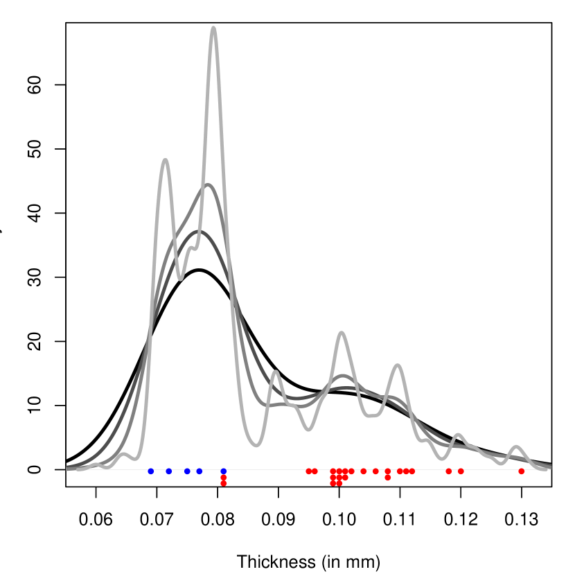
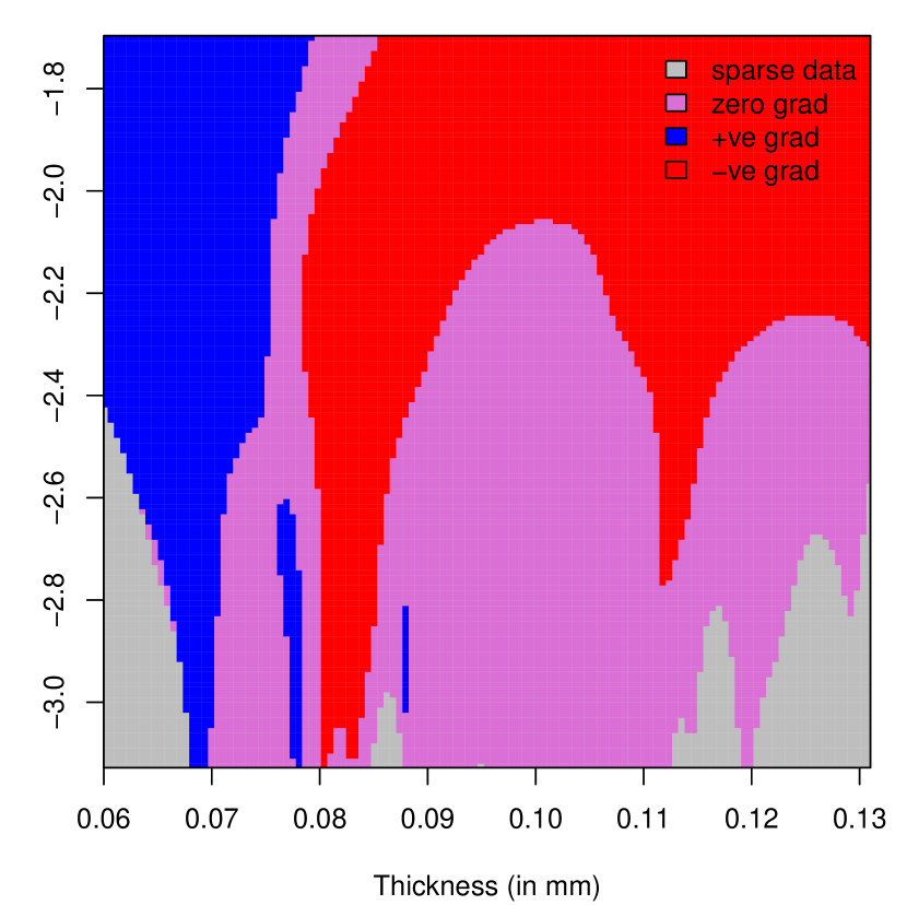
(a)
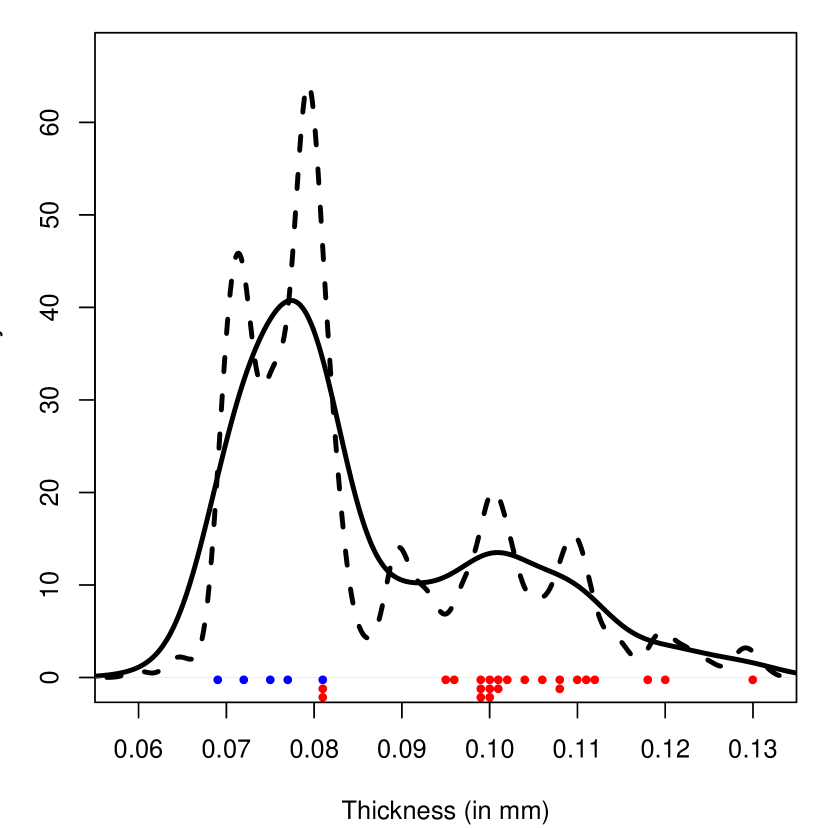
(d) (g)

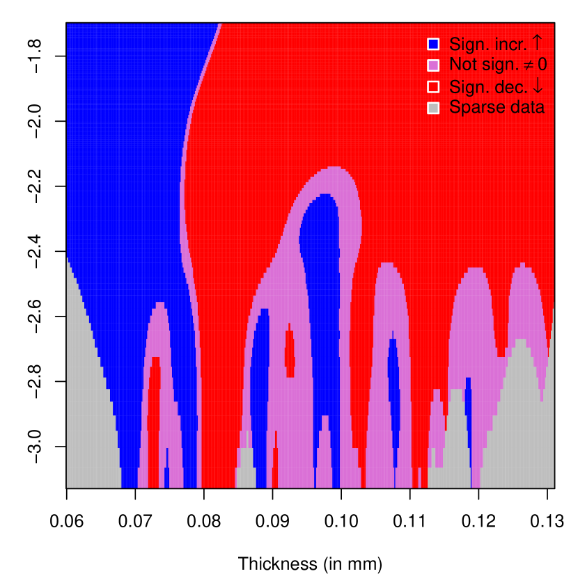
(b)
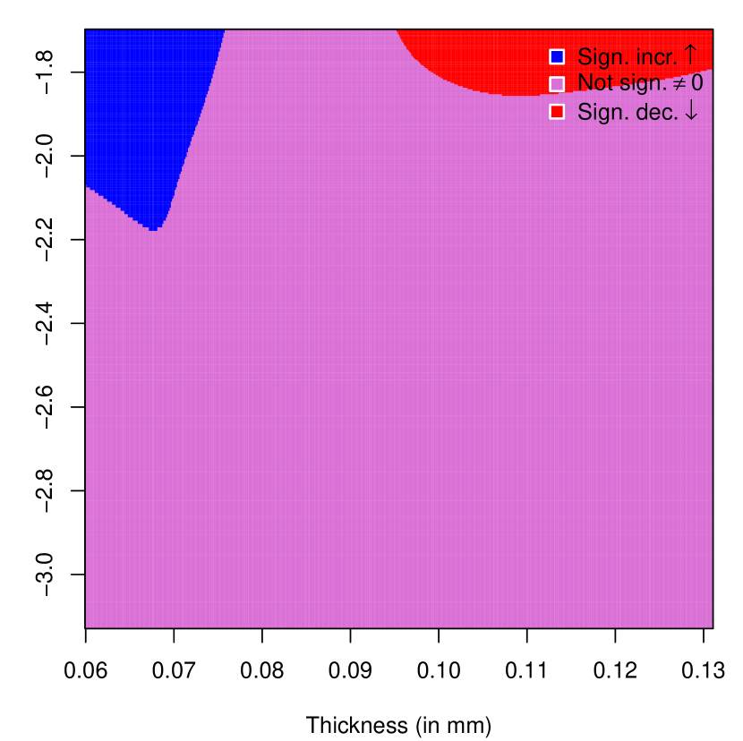
(e) (h)

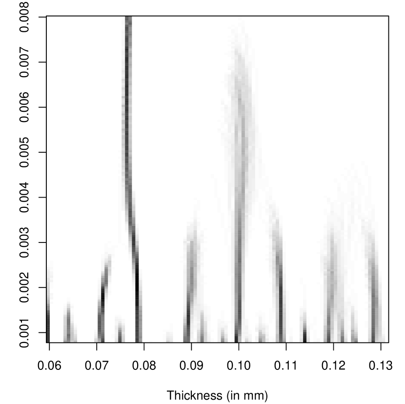
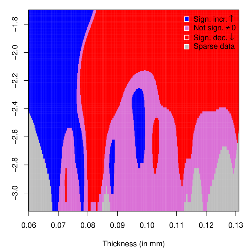
(c)
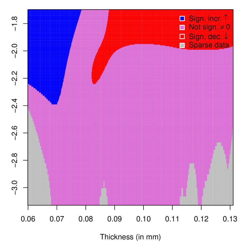
(f) (i)

Figure 1: Exploratory analisys for a sample of 485 stamps (1872 Hidalgo Issue of Mexico). In (a) and (d), kernel density estimators with Gaussian kernel and different bandwidths; the points represent stamps watermarked with LA+-F (blue) and Papel sellado (red). In (a), from dark to light grey, $h$ values: 0.007, 0.005, 0.003 and 0.001. In (d), $h=0.0039$ (rule of thumb -continuous line-) and $h=0.0012$ (plug–in rule -dashed line-, see Wand and Jones, 1995, Ch. 3). Mode tree (b) and mode forest (c) between the bandwidths $8\cdot 10^{-3}$ and $8\cdot 10^{-4}$. For each $h$, the estimated modes locations are identified by continuous lines in (b) and dark grey pixels in (c). The horizontal discontinuous lines (b) indicate how each mode splits. Panels (e)–(i): SiZer maps between $\log_{10}(h)=-1.7$ ($h=0.02$) and $\log_{10}(h)=-3.1$ ($h=8\cdot 10^{-4}$); given a value of $\log_{10}(h)$, modes can be detected by blue–red patterns. Obtained from feature package (g), using Gaussian, $q_{1}$ (e) and $q_{2}$ (f), and bootstrap, $q_{3}$ (h) and $q_{4}$ (i), quantiles.

In the mode tree, Minnotte and Scott (1993) created a tree diagram (similar to the dendrogram) representing, with continuous vertical lines, the modes locations (primary axis) of $\hat{f_{h}}$ for different bandwidth parameters $h$ (secondary axis). In addition, it represents, with horizontal dashed lines, how each mode splits into more modes as the bandwidth decreases (from top to bottom), showing the relationship between the new modes and the original modes from which they split.

As pointed out by Minnotte et al. (1998), the problem of the mode tree is the strong dependence on the available sample. That is the reason why the mode forest is constructed by computing the position of the estimated modes from different mode trees obtained from sampling with replacement the original sample. In order to facilitate the visualization of this exploratory method, the graphical window is divided in different (previously chosen) location–bandwidth (horizontal–vertical axis) pixels. Then, this tool represents the number of times that an estimated mode falls in each (location–bandwidth) pixel shading it proportionally to counts (large counts corresponding to darker pixels and low counts to lighter ones). Then, in the mode forest, modes are identified by dark grey regions.

A problem of the mode tree and the mode forest is that they do not identify which modes are artificially created by atypical data points. An exploratory tool that avoids this issue is the SiZer proposed by Chaudhuri and Marron (1999) and whose representation can be observed in Figure 1 (panels e, f, h and i). SiZer identifies the significant features of the density, by analysing the behaviour of the derivative of the kernel density estimation. For a given location (horizontal axis) and using a specified bandwidth parameter (vertical axis), the SiZer map represents where the smoothed curve is significantly increasing (blue colour), decreasing (red) or not significantly different from zero (orchid, a light tone of purple). Thus, for a given bandwidth, a significantly increasing region followed by a significantly decreasing region (blue–red pattern) indicates where a significant peak is present.

For determining the behaviour of the smoothed curve, fixing a location $x$ and a bandwidth $h$, the confidence limits of $\hat{f}_{h}^{\prime}(x)$ are of the form $\mbox{CI}^{\pm}(x,h)=\hat{f}_{h}^{\prime}(x)\pm\mbox{quantile}(\alpha)\cdot\widehat{\mbox{sd}}(\hat{f}_{h}^{\prime}(x))$, where $\widehat{\mbox{sd}}$ is the estimated standard deviation and $\alpha$ is the significance level. The estimation of the variance of $\hat{f}_{h}^{\prime}(x)$ is obtained in the following way

$$\widehat{\mbox{var}}\left(\hat{f}_{h}^{\prime}(x)\right)=\frac{1}{nh^{4}}S^{2}\left(K^{\prime}\left(\frac{x-X_{1}}{h}\right),...,K^{\prime}\left(\frac{x-X_{n}}{h}\right)\right),$$ (2)

where $S^{2}$ in (2) denotes the sample variance. In order to calculate the quantiles, Chaudhuri and Marron (1999) proposed four approximations: two based on Gaussian methods and two based on bootstrap techniques. The first proposal is based on pointwise Gaussian quantiles ($q_{1}$; Figure 1, panel e), where quantiles are calculated as $q_{1}(\alpha)=\Phi^{-1}\left(1-{\alpha}/{2}\right)$, being $\Phi^{-1}$ the normal quantile function. The second method provides approximate Gaussian quantiles simultaneous over $x$ ($q_{2}$; Figure 1, panel f) and they are defined as $q_{2}(\alpha;h)=\Phi^{-1}\left({1+(1-\alpha)^{1/m(h)}}/{2}\right)$. For each bandwidth, $m(h)$ are obtained from the Effective Sample Size (ESS, see Chaudhuri and Marron, 1999) in the following way

$$m(h)=\frac{n}{\overline{\mbox{ESS}}(x,h)},\quad\mbox{being }\mbox{ESS}(x,h)=\frac{\sum_{i=1}^{n}K\left(\frac{x-X_{i}}{h}\right)}{K(0)}$$ (3)

and $\overline{\mbox{ESS}}(x,h)$ the average mean over $x$ of the values of $\mbox{ESS}(x,h)$. Small values of ESS provide an indicative of areas with too sparse data for meaningful inference. For that reason, in the methods employing the ESS ($q_{2}$, $q_{3}$ and $q_{4}$), the significant features are just represented in the regions satisfying $x\in D_{h}=\{x:\mbox{ESS}(x,h)\geq n_{0}\}$ (remaining regions are marked with grey colour; see Figure 1, panels f, h and i). Then, the parameter $n_{0}$ (where Chaudhuri and Marron, 1999, proposed to use $n_{0}=5$) plays a fundamental role for removing the spurious modes created by atypical data points.

The two bootstrap quantiles are calculated from the following values

$$Z(x,h)^{*b}=\frac{\hat{f}_{h}^{\prime}(x)^{*b}-\hat{f}_{h}^{\prime}(x)}{\widehat{\mbox{sd}}(\hat{f}_{h}^{\prime}(x))},\mbox{ with }b=1,...,B,$$ (4)

where each $\hat{f}_{h}^{\prime}(x)^{*b}$ is calculated from a random sample generated drawn with replacement from the original sample. The third approach is a bootstrap quantile simultaneous over $x$, $q_{3}(\alpha;h)$ (Figure 1, panel h), and it is calculated with the empirical quantile $(1-\alpha/2)$ of the $B$ values ${\max}_{x\in D_{h}}|Z(x,h)^{*b}|$; with $b=1,...,B$. Finally, the fourth approach, also calculated from the quantities defined in (4), is the bootstrap quantile simultaneous over $x$ and $h$, $q_{4}(\alpha)$ (Figure 1, panel i), and it is defined as the empirical quantile $(1-\alpha/2)$ of the $B$ values ${\max}_{h}{\max}_{x\in D_{h}}|Z(x,h)^{*}|$; with $b=1,...,B$.

2.2 Testing procedures

Consider the testing problem presented in the Introduction. That is, given a sample $X_{1},\ldots,X_{n}$ from a random variable $X$ with unknown density $f$ with $j$ modes, and given a positive integer $k$, the goal is to test $H_{0}:\;j=k$ vs. $H_{a};\;j>k$. The testing methods, briefly described in this section and included in multimode, make use of one or both of the following concepts: the critical bandwidth and the excess mass.

2.3 Using a critical bandwidth

The critical bandwidth for a fixed $k$ was defined by Silverman (1981) as the smallest bandwidth such that the kernel density estimator in (1) has at most $k$ modes:

$$h_{k}=\inf\{h:\hat{f_{h}}\mbox{ has at most }k\mbox{ modes}\}.$$ (5)

This value can be used as a test statistic, as long as (1) is constructed with a Gaussian kernel, as proposed by Silverman (1981): $H_{0}$ is rejected for large values of $h_{k}$. For calibrating $h_{k}$, a bootstrap algorithm is employed, where the resamples $Y^{*b}_{i}=(1+h_{k}^{2}/\hat{\sigma}^{2})^{-1/2}X^{*b}_{i}$ (with $i\in\{1,\ldots,n\}$, being $n$ the sample size) are calculated from $B$ bootstrap samples $X^{*b}_{i}$ generated from $\hat{f}_{h_{k}}$, being $\hat{\sigma}^{2}$ the sample variance and with $b\in\{1,\ldots,B\}$. Hall and York (2001) proved that this bootstrap algorithm is not consistent and the authors suggested a correction for the unimodality test (for $k=1$), when $f$ has a bounded support or when the mode is located in a given closed interval $I$, defining the critical bandwidth as:

$$h_{\tiny{\mbox{HY}}}=\inf\{h:\hat{f_{h}}\mbox{ has exactly one mode in }I\}.$$ (6)

The authors also proposed using $h_{\tiny{\mbox{HY}}}$ as a test statistic and designed a bootstrap algorithm in this simplified scenario. However, the critical bandwidths for the bootstrap samples $h_{\tiny{\mbox{HY}}}^{*}$, calculated from $X^{*}$, are smaller than $h_{\tiny{\mbox{HY}}}$, so for an $\alpha$–level test, a correction factor $\lambda_{\alpha}$ to empirically approximate the p–value $\mathbb{P}(h_{\tiny{\mbox{HY}}}^{*}\leq\lambda_{\alpha}h_{\tiny{\mbox{HY}}}|\mathcal{X})\geq 1-\alpha$ must be considered. Two different methods were suggested for computing this $\lambda_{\alpha}$ factor (see Hall and York, 2001, for details). The first one is based on a polynomial approximation where after imposing a significance level $\alpha$, the correction factor $\lambda_{\alpha}$ is approximated with the following expression:

$$\lambda_{\alpha}=\frac{0.94029\alpha^{3}-1.59914\alpha^{2}+0.17695\alpha+0.48971}{\alpha^{3}-1.77793\alpha^{2}+0.36162\alpha+0.42423}.$$ (7)

The second one uses Monte Carlo techniques considering a simple unimodal distribution. In particular, Hall and York (2001) suggest to generate the resamples (of same sample size as the original data) obtained from a unimodal distribution resembling the sampled one and they claim that, in practice, normal distribution produce a good level accuracy.

Hall and York (2001) method should not be used in the general case of testing $k$–modality as the bootstrap test cannot be directly calibrated under this hypothesis, since it depends on the unknown quantities $f^{1/5}(t_{i})/|f^{\prime\prime}(t_{i})|^{2/5}$, where $t_{i}$ are the ordered turning points of $f$, with $i=1,\ldots,(2k-1)$.

As showed in Ameijeiras-Alonso et al. (2016), the critical bandwidth of Hall and York (2001) or Silverman (1981), when $f$ has a bounded support, also plays a relevant role when the goal is to estimate the modes locations. When the true number of modes is known, under some general assumptions, the kernel density estimation with the critical bandwidth provides a good estimation of the modes and antimodes locations.

A distribution estimation using the critical bandwidth of Silverman (1981) is also employed by Fisher and Marron (2001), who considered the following Cramér–von Mises test statistic for testing $k$–modality,

$$T_{k}=\overset{n}{\underset{i=1}{\sum}}\left(\hat{F}_{h_{k}}(X_{(i)})-\frac{2i-1}{2n}\right)^{2}+\frac{1}{12n},$$ (8)

being $\hat{F}_{h_{k}}(x)=\int_{-\infty}^{x}{\hat{f}_{h_{k}}(t)dt}$. $H_{0}$ is rejected for large values of $T_{k}$ (8), whose distribution is approximated by a bootstrap algorithm, where resamples are generated from $\hat{f}_{h_{k}}$.

2.4 Using an excess–mass statistic

The identification of a mode in a density estimate by finding a significant excess mass is the basic idea in the proposals by Müller and Sawitzki (1991), Cheng and Hall (1998) and Ameijeiras-Alonso et al. (2016). The empirical excess mass for $k$ modes and a constant $\lambda$ is defined as:

$$E_{n,k}(\mathbb{P}_{n},\lambda)=\underset{C_{1}(\lambda),...,C_{k}(\lambda)}{\mbox{sup}}\left\{\overset{k}{\underset{m=1}{\sum}}\mathbb{P}_{n}(C_{m}(\lambda))-\lambda||C_{m}(\lambda)||\right\},$$ (9)

where the supremum is taken over all families $\{C_{m}(\lambda):m=1,\cdots,k\}$ of closed intervals with endpoints at data points. $||C_{m}(\lambda)||$ denotes the measure of $C_{m}(\lambda)$ and $\mathbb{P}_{n}(C_{m}(\lambda))=(1/n)\sum_{i=1}^{n}\mathcal{I}(X_{i}\in C_{m}(\lambda))$, where $\mathcal{I}$ is the indicator function. The difference $D_{n,k+1}(\lambda)=E_{n,k+1}(\mathbb{P}_{n},\lambda)-E_{n,k}(\mathbb{P}_{n},\lambda)$ measures the plausibility of the null hypothesis, that is, large values of $D_{n,k+1}(\lambda)$ would indicate that $H_{0}$ is false. An example of the theoretical excess mass difference for a bimodal density is shown in Figure 2 for illustrative purposes. Using these differences, Müller and Sawitzki (1991) defined as the excess mass statistic for testing $H_{0}:\;j=k$,

$$\Delta_{n,k+1}=\underset{\lambda}{\max}\{D_{n,k+1}(\lambda)\},$$ (10)

Their proposal for testing unimodality is to calibrate this test statistic using a Monte Carlo calibration, where resamples are generated from the uniform distribution. The same approach was already proposed by Hartigan and Hartigan (1985) with the dip unimodality test, since both quantities (dip and excess mass) coincide up to a factor.

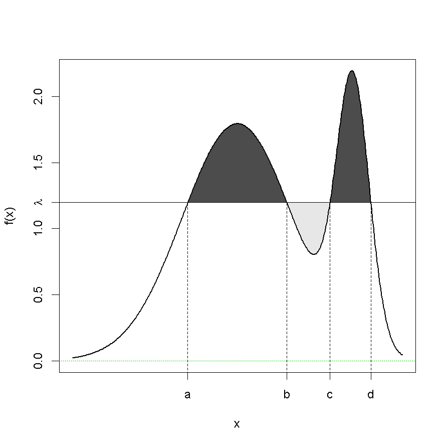
Figure 2: The excess mass for $k$ modes is the largest probability mass, exceeding a given level $\lambda$, when taking $k$ intervals. In this case, the excess mass for two modes is equal to the dark grey area (and obtained with the union of the intervals $[a,b]$ and $[c,d]$) and for one mode is equal to the dark grey minus the light grey area (and obtained with $[a,d]$). Then, in terms of excess mass, for the represented value of $\lambda$, the difference between assuming bimodality and unimodality is the light grey area.

The performance in practice of the calibration algorithm proposed for (10) was remarkably conservative and Cheng and Hall (1998) designed a bootstrap procedure for approximating the distribution of $\Delta_{n,2}$ under the hypothesis of unimodality generating the resamples from a family of parametric functions, guaranteeing an asymptotic correct behaviour. When analysing Cheng and Hall (1998) proposal in simulated scenarios (see Ameijeiras-Alonso et al., 2016), the calibration of the test was not satisfactory in the “complicated” unimodal models due the lack of flexibility of this parametric approach. Also, extending this test to the general case of testing $k$–modality is not an easy task. For those reasons, a completely nonparametric alternative for testing $H_{0}:\;j=k$ vs. $H_{a}:\;j>k$ has been proposed by Ameijeiras-Alonso et al. (2016). Their method consist in calibrating the excess mass statistic given in (10) using a bootstrap procedure, where the resamples are generated from (a modified version of) $\hat{f}_{h_{k}}$. The modification of the kernel density estimator ensures the correct calibration of this test, under some regularity conditions (similar to those ones needed in Cheng and Hall, 1998). Although, in general, the Ameijeiras-Alonso et al. (2016) proposal presents a correct behaviour even when the sample size is “small” ($n=50$), when knowing the compact support $I$ where the modes and antimodes lie, the Hall and York (2001) bandwidth can be employed (for generating the resamples), improving the results of this test.

When deciding which proposal should be chosen, it must be considered that an asymptotic correct behaviour is just expected in the unimodality tests of Hall and York (2001) (when $f$ has a bounded support or when employing the compact support $I$) and Cheng and Hall (1998) and in the multimodality test of Ameijeiras-Alonso et al. (2016). A complete simulation study comparing all the aforementioned proposals is provided in Ameijeiras-Alonso et al. (2016), showing that the other proposals (Silverman, 1981; Fisher and Marron, 2001) for testing $H_{0}:\;j=k$ vs. $H_{a}:\;j>k$, when $k>1$, exhibit an unsatisfactory behaviour.

3 Using multimode

A complete description of the multimode package capabilities is provided in this section. Specifically, the package includes the datasets and the functions shown in Table 1. First, the different datasets available in the package will be described. Second, the usage of different functions for exploring the number of modes will be illustrated. Finally, the functions for testing multimodality and estimating the location of modes and antimodes will be introduced.

Dataset	Description
acidity	Acid–neutralizing capacity
chondrite	Percentage of silica in chondrite meteors
enzyme	Blood enzymatic activity
galaxy	Velocities of galaxies
geyser	Waiting time between geyser eruptions
stamps	Stamps thickness
Function	Description
critbw	Critical bandwidth computation
excessmass	Excess mass statistic
locmodes	Location of modes and antimodes
modeforest	Mode forest
modetest	Test for the number of modes
modetree	Mode tree
nmodes	Number of modes
sizer	SiZer map

Table 1: Summary of multimode package contents.

3.1 Data description

The package multimode includes some classical datasets for which determining the number of different groups in the sample and/or exploring the location of modes and antimodes are relevant issues. The first dataset, acidity, analysed by Crawford (1994), contains, on the log scale, the Acid–Neutralizing Capacity (ANC) measured in a sample of 155 lakes in North–Central Wisconsin (USA). ANC describes the capability of a lake to absorb acid, where low ANC values may lead to a loss of biological resources. The dataset chondrite, included in Table 2 of Good and Gaskins (1980), gathers the percentage silica (in %) in 22 chondrite meteors. The dataset enzyme, introduced by Bechtel et al. (1993), collects a sample with the distribution of enzymatic activity in the blood, for an enzyme involved in the metabolism of carcinogenic substances. The dataset galaxy provides the velocities in km/sec of different galaxies (diverging away from our own galaxy) from the unfilled survey of the Corona Borealis region. In this dataset introduced by Postman et al. (1986) and further studied by Roeder (1990), multimodality is an evidence for voids and superclusters in the universe. The dataset in geyser presents the interval times between the starts of the geyser eruptions observed during different periods in the Old Faithful Geyser in Yellowstone National Park, Wyoming, USA. The included periods are: October 1980, obtained from Table 3 of Härdle (2012) and the supplementary material of Weisberg (2005); and August 1985, from Table 1 in Azzalini and Bowman (1990). Finally, the dataset stamps, analysed in Izenman and Sommer (1988), consists of thickness measurements (in millimetres) of 485 unwatermarked used white wove stamps of the 1872 Hidalgo stamp issue of Mexico. All of them had an overprint with the year (1872 or either an 1873 or 1874) and some of them were watermarked (Papel Sellado or LA+-F), being this information also included inside stamps. Since the stamps value depends on its scarcity, it is of importance to determine the number of available groups in a particular stamp issue. For this particular stamp issue, although the watermark is some stamps (in 29 of 485) helps to conclude that there are at least two groups, the question about the number of groups can be answered analysing the underlying number of modes.

Some of these datasets (acidity, enzyme, galaxy or stamps) were used in the statistical literature for illustrating mixtures of parametric models. The nonparametric (both exploratory and inferential) tools included in multimode could be seen as a preliminary tool for determining the number of modes. Some references can be found in McLachlan and Peel (2000) or Richardson and Green (1997). In other datasets (chondrite, geyser or stamps), testing or exploring the number of modes is an important problem per se. Some examples of their application can be found in Chaudhuri and Marron (1999), Müller and Sawitzki (1991) or Scott (2015, Sect. 9.2). In the subsequent sections, the stamps dataset will be used for illustrating the functions available in the multimode package.

3.2 Exploring data with multimode

When the objective is to explore the number of modes in a sample, a simple solution might be to observe the number of peaks in the kernel density estimation for different values of $h$. In order to facilitate this task, using the Gaussian kernel and a given bandwidth parameter bw, the function nmodes computes the estimated number of modes in the real line or in a support bounded by lowsup and uppsup. This kernel density estimation is calculated in n equally spaced points of the variable for computational reasons (as in the density function from the stats package). For instance, using the code below, it can be seen that the estimated number of modes using the rule of thumb and the plug–in rule (bw.nrd0 and bw.SJ from the stats package and illustrated in Figure 1, panel d) is, respectively, two and nine.

R> data(stamps)
R> bwRT <- bw.nrd0(stamps) ; bwPI <- bw.SJ(stamps)
R> nmodes(data=stamps,bw=bwRT,lowsup=-Inf,uppsup=Inf,n=2^15)
R> nmodes(data=stamps,bw=bwPI,lowsup=-Inf,uppsup=Inf,n=2^15)

Based on the idea of exploring the number of modes (and their location) for different values of $h$, the three different graphical tools, presented in Section 2.1, have been implemented in multimode: modetree, modeforest and sizer. The outputs from these exploratory functions and the arguments used for their computation are detailed below. The common characteristics, in the three of them, are: the exploratory features will be calculated in a finite number of grid points (the common argument is the first element of gridsize); the number of modes will be determined according to a value of $h$ and the employed bandwidth values can be chosen by the practitioner (bws, cbw1, cbw2 and the second element gridsize); a graphical display is generated (or added to the current graphic) with different plot arguments (display, logbw, xlab, ylab); an output related with the modes locations is returned.

The different exploratory tools (modetree, modeforest and sizer) include three options for providing the bandwidths. The first one is to use a range of bandwidth parameters in the argument bws and the exploratory tool is computed in a grid of $h$ between the given values and size equal to the second element of the argument gridsize. By default, a grid of size 151 is computed between a lower bandwidth equal to twice the distance between the grid points used for estimating the density and upper bandwidth equal to the data range. The second option considers the critical bandwidths for cbw1 and cbw2 modes as the range of bandwidths. The third method allows to include a vector of bandwidths in the argument bws with size greater than two. Then, these exploratory tools are represented (using a $\log_{10}$ scale for the bandwidths if logbw=TRUE) when the argument display is TRUE with the titles in the x and y axis provided by xlab and ylab, as usual.

The mode tree introduced by Minnotte and Scott (1993) and implemented in the function modetree, shows with continuous lines the estimated mode locations for each bandwidth. For modetree, the first element of gridsize is equal to the number of equally spaced points at which the density is to be estimated. Moreover, the mode tree can be added to another plot when the argument addplot is TRUE. Also, the color lines in the mode tree can be chosen with the argument col.lines. Below, an example with the code lines for computing the mode tree for the stamps dataset between the bandwidths $8\cdot 10^{-4}$ and $8\cdot 10^{-3}$ is shown (its representation appears in Figure 1, panel b).

R> mtstamps <- modetree(data=stamps,bws=c(0.0008,0.008),
+    gridsize=c(512,151),cbw1=NULL,cbw2=NULL,display=TRUE,logbw=FALSE,
+    addplot=FALSE,xlab="Thickness (in mm)",ylab=NULL,col.lines="black")
R> names(mtstamps)

[1] "locations"  "bandwidths"

This function returns a list containing the following components: locations, a matrix with the estimated modes locations for each bandwidth; and bandwidths, the bandwidths employed for computing the mode tree. The plot and the argument locations returned by the function modetree can be useful for exploring where the different modes are located when the number of modes is not clear and a further insight on the data distribution is required. In this case, the principal mode appears between the values 0.0765 and 0.0793, the secondary mode between 0.0986 and 0.1011, and so forth.

The mode forest, introduced by Minnotte et al. (1998), is provided by modeforest. This graphical tool is generated by looking simultaneously at a collection of mode trees generated by the original sample and B random resamples drawn with replacement from the original one.

For the modeforest and sizer, the first element of gridsize is equal to the number of grid points in the horizontal (values of the variable) axis. In both cases, the horizontal values plotted are bounded by the interval (from,to), being this interval equal to the data range by default. In the modeforest function, the number of equally spaced points at which the density is to be estimated is chosen by the argument n. The mode forest for the stamps dataset between the bandwidths $8\cdot 10^{-4}$ and $8\cdot 10^{-3}$ (represented in Figure 1, panel c) can be obtained as follows:

R> mfstamps <- modeforest(data=stamps,bws=c(0.0008,0.008),
+    gridsize=c(100,151),B=99,n=512,cbw1=NULL,cbw2=NULL,display=TRUE,
+    logbw=FALSE,from=NULL,to=NULL,xlab="Thickness (in mm)",ylab=NULL)
R> names(mfstamps)

[1] "modeforest" "range.x"    "range.bws"

The output is a matrix modeforest including the percentage of times that an estimated mode falls in each location–bandwidth pixel. The functions modeforest and sizer return range.x (the employed location values to represent the mode forest or the SiZer map) and range.bws (the bandwidths used for computing the exploratory tool). In the modeforest plot, modes can be detected observing the dark grey vertical traces, but one should be careful with the very dark areas (as the one next to 0.06) since, due to the resampling algorithm, it is possible that spurious modes (created by some atypical data points) may seem visually more prominent than real modes (as pointed out by Minnotte et al., 1998). Observing Figure 1 (panel c), the mode forest suggests at least seven modes for the stamps dataset.

With the sizer function the assessment of SIgnificant ZERo crossing of the derivative of the smoothed curve is computed for a given sample. In each location–bandwidth pixel, the SiZer map shows the significant features of the smoothed curve using, by default, the colours described in Section 2.1, but they can be replaced using the col.sizer argument. For analysing the behaviour of the curve, the four quantile approximations proposed by Chaudhuri and Marron (1999) are implemented in the sizer function using the argument method. The available quantiles are: the pointwise Gaussian quantiles ($q_{1}$), when method=1; approximate simultaneous over location $x$ Gaussian quantiles ($q_{2}$), when method=2; bootstrap quantile simultaneous over location $x$ ($q_{3}$), when method=3; and bootstrap quantile simultaneous over (location and bandwidth) $x$ and $h$ ($q_{4}$), when method=4. Bootstrap quantiles $q_{3}$ and $q_{4}$ are computed generating B random samples drawn with replacement from the sample. In methods $q_{2}$, $q_{3}$ and $q_{4}$; grey colour (by default) is employed when the Effective Sample Size in (3) is less than the value n0. A legend indicating the meaning of the different colours is also provided in the plot position given in poslegend when the argument addlegend is TRUE. The different SiZer maps for the stamps dataset between the bandwidths $8\cdot 10^{-4}$ and $0.02$ (represented in Figure 1; panels e, f, h and i) can be obtained as shown below (varying the value of method between 1 and 4). For computing the quantiles $q_{2}$, $q_{3}$ and $q_{4}$ it was taken n0=5 and the number of bootstrap replicas in methods $q_{3}$ and $q_{4}$ is B=500.

R> sizerstamps <- sizer(data=stamps,method=1,bws=c(0.0008,0.02),
+    gridsize=NULL,alpha=0.05,B=NULL,n0=NULL,cbw1=NULL,cbw2=NULL,
+    display=TRUE,logbw=TRUE,from=NULL,to=NULL,col.sizer=NULL,
+    xlab="Thickness (in mm)",ylab=NULL,addlegend=TRUE,
+    poslegend="topright")
R> names(sizerstamps)

[1] "sizer"     "lower.CI"  "estimate"  "upper.CI"  "ESS"
[6] "range.x"   "range.bws"

Apart from the already described arguments, sizer returns a list with five matrices containing different information in each location–bandwidth pixel: sizer, with the significant behaviours of the smoothed curve in each location–bandwidth pixel (1: significantly decreasing, 2: not significantly different from zero, 3: significantly increasing or 4: low data for meaningful inference); lower.CI with the lower limits of the confidence interval, $\mbox{CI}^{-}(x,h)$; estimate, with the derivative values of the kernel density estimation, $\hat{f}_{h}^{\prime}(x)$; upper.CI with the upper limits of the confidence interval, $\mbox{CI}^{+}(x,h)$; and ESS, with the Effective Sample Size.

As noted before, in the SiZer maps (represented in Figure 1; panels e, f, h and i), by default, blue colour indicates locations where, for a given bandwidth, the smoothed curve is significantly increasing, red colour shows where it is significantly decreasing and orchid indicates where it is not significantly different from zero. Then, focusing on $\log_{10}(h)$ values, modes can be detected by blue–red patterns. In this case, the SiZer maps computed with Gaussian quantiles just detect, at most, one mode around 0.08. The conclusion with those ones constructed with bootstrap confidence intervals vary with the bandwidth. For all the bandwidth values, both methods capture a principal mode before the value 0.08 and for several bandwidth parameters is also detected a secondary mode around 0.10. The third and the fourth mode (around 0.09 and 0.11) that appears in the mode tree (Figure 1, panel b) are only significant modes for some bandwidth parameters for $q_{3}$. Finally, both methods, $q_{3}$ and $q_{4}$, detect another mode near 0.07 for some bandwidth values. Then, depending on the bandwidth parameter, the conclusion using the quantile $q_{3}$ is that there are between one and five modes (in order of appearance, around 0.08, 0.10, 0.09, 0.11 and 0.07), while $q_{4}$ detects between one and three modes (around 0.08, 0.10 and 0.07).

3.3 Testing and locating modes with multimode

The multimode package has implemented all the test presented in the Section 2.2. In particular, it allows to compute the critical bandwidth of Silverman (1981) and Hall and York (2001) (with the function bw.crit) and the excess mass of Müller and Sawitzki (1991) (with excessmass). Their associated p–values can be also obtained, with modetest, using different testing proposals. For the three functions (bw.crit, excessmass and modetest), the investigated number of modes can be specified in the argument mod0.

For bw.crit and for the testing proposals using the critical bandwidth in modetest, when the compact support is unknown, the critical bandwidth introduced by Silverman (1981) is computed and if the finite values of the support limits are provided (via arguments lowsup and uppsup) the one proposed by Hall and York (2001) is calculated. Both arguments should be used in modetest when employing the Hall and York (2001) proposal or for computing the new proposal when the compact support is known (see Section 2.4). As in the nmodes function, the number of equally spaced points at which the density is to be estimated is chosen by the argument n. Since a dichotomy method is employed for computing the critical bandwidth, the parameter tol is used to determine a stopping time in such a way that the error committed in the computation of the critical bandwidth is less than tol.

For excessmass and in the testing proposals using the excess mass in modetest, when there are repeated data in the sample or the distance between different pairs of data points shows ties, a data perturbation is applied. This modification is made in order to avoid the induced discretization of the data which has important effects on the computation of this test statistic. The perturbed sample is obtained by adding a sample from the uniform distribution in the support minus/plus a half of the minimum of the positive distances between two sample points.

Since the excess mass for one mode is twice the dip, this equality can be used for a “fast” computation of the excess mass for one mode. When mod0 is greater than one and the sample size is “large”, a two–steps approximation (approximate=TRUE) can be performed in order to improve the computational time efficiency. This two–steps approximation is achieved creating two grids of values of size the elements in gridsize. First, since the possible $\lambda$ candidates for maximizing $D_{n,k+1}(\lambda)$ can be directly obtained from the $C_{m}(\lambda)$ sets that could maximize $E_{n,k+1}$ and $E_{n,k}$ (see Supplementary Material in Ameijeiras-Alonso et al., 2016), the possible values of $\lambda$ are computed by looking to the empirical excess mass function in some endpoints candidates for $C_{m}(\lambda)$ (the number of employed points is equal to the first element of gridsize) and also in the $\lambda$ values associated to the empirical excess mass for one mode. Once a $\lambda$ maximizing the approximated values of $D_{n,k+1}(\lambda)$ is chosen, in order to obtain the approximation of the excess mass test statistic, in its neighbourhood, a grid of possible $\lambda$–values is created, being its length equal to the second element of gridsize, and the exact value of $D_{n,k+1}(\lambda)$ is calculated for these values of $\lambda$ (using the algorithm proposed by Müller and Sawitzki, 1991).

An illustration with the stamps dataset is shown below. First, the critical bandwidth of Silverman (1981) and Hall and York (2001), in the interval $I=[0.04,0.15]$, is computed for two modes. Second, the exact and approximated version of the excess mass test statistic of Müller and Sawitzki (1991) for two modes are obtained.

R> bw.crit(data=stamps,mod0=2,lowsup=-Inf,uppsup=Inf,n=2^15,tol=10^(-5))
R> bw.crit(data=stamps,mod0=2,lowsup=0.04,uppsup=0.15,n=2^15,tol=10^(-5))
R> excessmass(data=stamps,mod0=2,approximate=FALSE)
R> excessmass(data=stamps,mod0=2,approximate=TRUE,gridsize=c(20,20))

Once the different test statistics are computed, the number of modes for the underlying density of a given sample can be tested with the function modetest. The different proposals that can be used for testing the number of modes (using the argument method) are those ones introduced in Section 2.2. The available methods, based on the critical bandwidth (see Section 2.3), include: Silverman (1981) (SI), Hall and York (2001) (HY) and Fisher and Marron (2001) (FM). Based on the excess mass (Section 2.4): Hartigan and Hartigan (1985) (HH, equivalent to the proposal of Müller and Sawitzki, 1991), Cheng and Hall (1998) (CH) and the new proposal of Ameijeiras-Alonso et al. (2016) (ACR) is also included. For calculating the corresponding p–value, all the available proposals require bootstrap or Monte Carlo resamples and the number of replicates can be specified with the argument B.

For SI, HY and ACR proposals, the argument submethod is available. In the SI case, two resampling methods are implemented: when submethod=1, the resamples are generated from the rescaled bootstrap resamples as proposed by Silverman (1981) (see Section 2.3); if submethod=2, the resamples are generated from $\hat{f}_{h_{k}}$. In the ACR method, the approximated version of the excess mass can be employed, for computational time efficiency reasons, by setting submethod=2; if submethod=1, then the exact value of the excess mass test statistic is computed.

As pointed out in Section 2.2, the bounded support (lowsup and uppsup) is necessary when the Hall and York (2001) proposal (HY) is employed and $f$ has not a compact support and it can be also used with the ACR proposal. In the ACR case, the parameter tol2 is the accuracy required in the integration of the calibration function when the compact support is known (see Ameijeiras-Alonso et al., 2016). As mentioned in Section 2.3, a level correction (achieved with the $\lambda_{\alpha}$ factor) is needed in the bootstrap procedure of Hall and York (2001). The two suggested approximations for its computation are provided in the HY test using the argument submethod. The submethod 1 corresponds with the asymptotic correction of Silverman (1981) test based on the limiting distribution of the test statistic, i.e. it consists in using equality (7). In equation (7), since the value of $\lambda_{\alpha}$ depends on $\alpha$, when submethod=1, the significance level must be previously determined with alpha. The submethod 2 is based on Monte Carlo techniques where the resamples are generated from the normal distribution. For this reason, when submethod=2, the number of normal–distributed samples (nMC) and the number of bootstrap resamples (BMC) used for computing the p–value in each Monte Carlo sample are needed.

Finally, the modetest function includes the argument full.result. When this argument equals TRUE, the function returns a list with both, the test statistic (statistic) and the associated p–value (p.value); when it is FALSE, just the p.value is returned.

The different p–values obtained for the stamps dataset with the Ameijeiras-Alonso et al. (2016) proposal (calculating the exact value of the excess mass) are reproduced in Table 3 and they can be obtained as follows (varying the value of mod0 between 1 and 9):

R> modeteststamps <- modetest(data=stamps,mod0=1,method="ACR",B=500,
+    full.result=TRUE,submethod=1,n=2^10,tol=10^(-5))
R> names(modeteststamps)

[1] "p.value"   "statistic"

Assuming that the compact support for the stamps dataset is $I=[0.04,0.15]$ (see Izenman and Sommer, 1988), the modification of the Ameijeiras-Alonso et al. (2016) proposal with known compact support can be obtained as follows

R> modetest(data=stamps,mod0=1,method="ACR",B=500,full.result=FALSE,
+    submethod=1,lowsup=0.04,uppsup=0.15,n=2^10,tol=10^(-5),tol2=10^(-5))

The p–values of the other proposals allowing for testing a general number of modes (SI and FM) are obtained with the below code lines (varying the value of mod0 between 1 and 9).

R> modetest(data=stamps,mod0=1,method="SI",B=500,full.result=FALSE,
+    submethod=1,n=2^10,tol=10^(-5))
R> modetest(data=stamps,mod0=1,method="FM",B=500,full.result=FALSE,
+    n=2^10,tol=10^(-5))

The other critical bandwidth based method, HY, should only be used for testing unimodality when when $f$ has a bounded support or when the modes and antimodes lie in a known closed interval $I$, in this case $I=[0.04,0.15]$. The test with both alternatives for approximating the $\lambda_{\alpha}$: a first approach based on a polynomial approximation (submethod=1) and a second option using Monte Carlo techniques (submethod=2), can be computed as follows:

R> modetest(data=stamps,method="HY",B=500,full.result=FALSE,lowsup=0.04,
+    uppsup=0.15,n=2^10,tol=10^(-5),submethod=1,alpha=0.05)
R> modetest(data=stamps,method="HY",B=500,full.result=FALSE,lowsup=0.04,
+    uppsup=0.15,n=2^10,tol=10^(-5),submethod=2,nMC=100,BMC=100)

The p–values of the unimodality test based on the excess mass (HH and CH) can be obtained with the following code lines:

R> modetest(data=stamps,method="HH",B=500,full.result=FALSE)
R> modetest(data=stamps,method="CH",B=500,full.result=FALSE)

Table 2 shows the p.values obtained for all the unimodality tests available. Note that, in the ACR case, submethod=2 was not employed as when mod0=1 the exact version of the excess mass is computed in a more efficient way, then it does not make sense to use its approximated version. For all of them the null hypothesis of unimodality is rejected for a significance level $\alpha=0.05$.

method	SI		HY		FM	HH	CH	ACR
submethod	1	2	1	2				1
P–value	0.018	0.006	0	0	0	0.030	0	0

Table 2: P–value obtained using different proposals for testing unimodality, with $B=500$ resamples. The employed testing procedures are: SI (using the rescaled, submethod 1, and the non–rescaled, submethod 2, bootstrap resamples), HY (using the two suggested approximations of $\lambda_{\alpha}$), FM, HH, CH and ACR (employing the exact version of the excess mass test statistic).

The results for the tests (SI, FM and ACR) that allow testing $k$–modality, with $k>1$, are displayed in Table 3 (with $k$ between one and nine). In the case of the FM proposal, for reproducing the Fisher and Marron (2001) results, the stamps data were also perturbed as done with the excessmass function. Similar results are obtained for the SI proposal, with and without data perturbation when using submethod=1 or submethod=2; and for the ACR proposal, independently of using or not the known support $I=[0.04,0.15]$. Fixing a significance level $\alpha=0.05$, there is not a clear conclusion when using SI and FM. In the SI case the null hypothesis is not rejected for $k=2,3,7,8,9$ and for the FM, using the perturbed sample, it is not rejected just for $k=7$. While, in the single proposal that is well calibrated (ACR, see Ameijeiras-Alonso et al., 2016), the null hypothesis is rejected until $k=3$ and it is not for $k\geq 4$, suggesting that the number of modes is equal to 4.

$k$	1	2	3	4	5	6	7	8	9
SI	0.018	0.394	0.090	0.008	0.002	0.002	0.488	0.346	0.614
FM	0	0.006	0	0	0	0	0	0	0
FM*	0	0	0	0	0	0	0.096	0.014	0.046
ACR*	0	0.022	0.004	0.506	0.574	0.566	0.376	0.886	0.808

Table 3: P–value obtained using different proposals for testing $k$–modality, with $k$ between 1 and 9, employing $B=500$ resamples. The employed testing procedures are: SI over the original sample (using the rescaled bootstrap resamples), FM over the original sample, FM over the perturbed sample (FM*) and ACR over the perturbed sample (employing the exact version of the excess mass test statistic).

Once the number of modes is known, the function locmodes provides the estimation of the locations of modes and antimodes and their estimated density value. In this case, the compact support of the variable (which is known) can be used to obtain a good estimator of the modes and antimodes locations (see Section 2.3). In other scenarios, one should be careful about the conclusions as the critical bandwidth of Silverman (1981) may create artificial modes in the tails (see Hall and York, 2001).

The arguments for locmodes function include those ones mentioned in the bw.crit function: mod0, lowsup, uppsup, n and tol. It also allows the representation of the estimation (for the number of modes indicated in mod0) of the density, modes and antimodes with the argument display. The remaining graphical arguments (addplot, xlab, ylab, addLegend, posLegend) were already described in the modetree and sizer functions.

The estimation of the modes and antimodes locations and their density value, assuming four (mod0=4, Ameijeiras-Alonso et al., 2016) and seven (mod0=7, Izenman and Sommer, 1988) modes, can be obtained as follows (their representation is provided in Figure 3):

R> lms <- locmodes(data=stamps,mod0=4,lowsup=0.04,uppsup=0.15,n=2^15,
+    tol=10^(-5),display=TRUE,addplot=FALSE,xlab="Thickness (in mm)",
+    ylab=NULL,addLegend=TRUE,posLegend="topright")
R> names(lms)

[1] "locations" "fvalue"    "cbw"

(a)

(b)

Figure 3: Estimation of the density, modes and antimodes for the sample of 485 stamps from the 1872 Hidalgo Issue of Mexico, obtained with the function locmodes for mod0=4 (left) and mod0=7 (right) modes.

This function returns locations, a vector with the estimated locations of modes (odd positions of the vector) and antimodes (even positions); fvalue, a vector with their estimated density values; and cbw, the critical bandwidth of the sample for mod0 modes. Regarding the obtained results assuming that the distribution has four modes, the estimated modes (odd positions of locations) are: 0.07857, 0.09065, 0.1006 and 0.1083.

The results obtained after applying the modetest function can be helpful for having a better interpretation of the SiZer map (Figure 1, panels e, f, h and i). If the conclusion is that there are four modes, the most plausible results are obtained with the bootstrap quantiles $q_{3}$ and, in that case, the estimated modes (in locmodes) coincide with those ones observed when a value of $\log_{10}(h)$ close to $-2.7$ is taken.

4 Discussion

The available functions of the R package multimode were described in this paper. This package was developed with the objective of making the mode testing and exploring procedures, for linear data, accessible for the scientific community, and therefore, enabling its use in practical problems. As pointed out in Section 1, there are many examples in different disciplines where the identification of the number (and location) of modes is important per se, or as a previous step for applying other procedures. Package multimode contains nonparametric graphical tools for (visually) exploring the number of modes and their estimated location and also testing proposals for determining the number of modes in the data distribution.

Up to the author’s knowledge, multimode is the only statistical package that allows for testing, in a nonparametric way, a general number of modes and, also, it is the only one providing a well–calibrated method for testing unimodality. Obtaining a final p–value, instead of a graphical tool, can be useful when the objective is, e.g. to obtain conclusions about the number of modes in a systematic manner. This is the case of McQuillan et al. (2014) or Joubert et al. (2016) where they performed several times the unimodality test of Hartigan and Hartigan (1985), dividing the sample, in the first case, in a temperature bin, and in the second case, in a collection of different CpGs (see Section 1). The combination of this package with other False Discovered Rate techniques (see, e.g. p.adjust from the stats package) allows to account for the multiple testing problem when the objective is to determine the number of modes.

So far, multimode includes just exploratory and testing procedures for mode assessment for real random variables. However, the ideas in Ameijeiras-Alonso et al. (2016) can be extended to settings where there is a natural nonparametric estimator. This is the case with circular random variables, for instance. As mentioned before, in R, there are already some packages allowing for exploring the number of modes in this setting, such as the circular version of the SiZer map implemented in NPCirc (see Oliveira et al., 2014b). Referring to the testing approach, Fisher and Marron (2001) already introduced a proposal for determining the number of modes in this circular setting. In particular, they suggested to use the circular version of the $T_{k}$ test statistic, namely the $U^{2}$ of Watson (1961). Future extensions of the multimode package could include some procedures for assessing the number of modes in other settings, such as the mentioned proposal of Fisher and Marron (2001).

5 Acknowledgements

The authors gratefully acknowledge the support of Project MTM2016–76969–P from the Spanish State Research Agency (AEI) and the European Regional Development Fund (ERDF), IAP network from Belgian Science Policy. Work of J. Ameijeiras-Alonso has been supported by the PhD Grant BES–2014–071006 from the Spanish Ministry of Economy, Industry and Competitiveness.

References

- Ameijeiras-Alonso et al. (2016) Ameijeiras-Alonso, J., Crujeiras, R. M., and Rodríguez-Casal, A. (2016). Mode testing, critical bandwidth and excess mass. arXiv preprint arXiv:1609.05188. Submitted.
- Ameijeiras-Alonso et al. (2018) Ameijeiras-Alonso, J., Crujeiras, R. M., and Rodríguez-Casal, A. (2018). multimode: Mode Testing and Exploring. R package version 1.1. URL https://CRAN.R-project.org/package=multimode
- Azzalini and Bowman (1990) Azzalini, A., and Bowman, A. W. (1990). A look at some data on the Old Faithful geyser. Applied Statistics, 39, 357–365.
- Bechtel et al. (1993) Bechtel, Y. C., Bonaiti-Pellie, C., Poisson, N., Magnette, J., and Bechtel, P. R. (1993). A population and family study N-acetyltransferase using caffeine urinary metabolites. Clinical Pharmacology & Therapeutics, 54, 134–141.
- Benaglia et al. (2009) Benaglia, T., Chauveau, D., Hunter, D. R., and Young, D. (2009). mixtools: An R Package for Analyzing Finite Mixture Models. Journal of Statistical Software, 32, 1–29. URL http://www.jstatsoft.org/v32/i06/
- Chaudhuri and Marron (1999) Chaudhuri, P., and Marron, J. S. (1999). SiZer for Exploration of Structures in Curves. Journal of the American Statistical Association, 94, 807–823.
- Cheng and Hall (1998) Cheng, M. Y., and Hall, P. (1998). Calibrating the excess mass and dip tests of modality. Journal of the Royal Statistical Society. Series B, 60, 579–589.
- Colombo et al. (2015) Colombo, M. G., Franzoni, C., and Rossi-Lamastra, C. (2015). Internal social capital and the attraction of early contributions in crowdfunding. Entrepreneurship Theory and Practice, 39, 75–100.
- Crawford (1994) Crawford, S. L. (1994). An application of the Laplace method to finite mixture distributions. Journal of the American Statistical Association, 89, 259–267.
- Dümbgen and Walther (2008) Dümbgen, L., and Walther, G. (2008). Multiscale inference about a density. The Annals of Statistics, 36, 1758–1785.
- Duong et al. (2008) Duong, T., Cowling, A., Koch, I., and Wand, M. P. (2008). Feature significance for multivariate kernel density estimation. Computational Statistics & Data Analysis, 52, 4225–4242.
- Duong and Wand (2015) Duong, T., and Wand, M. (2015). feature: Local Inferential Feature Significance for Multivariate Kernel Density Estimation. R package version 1.2.13. URL https://CRAN.R-project.org/package=feature
- Fisher and Marron (2001) Fisher, N. I., and Marron, J. S. (2001). Mode testing via the excess mass estimate. Biometrika, 88, 419–517.
- Freeman and Dale (2013) Freeman, J. B., and Dale, R. (2013). Assessing bimodality to detect the presence of a dual cognitive process. Behavior research methods, 45, 83–97.
- Godtliebsen et al. (2002) Godtliebsen, F., Marron, J., and Chaudhuri, P. (2002). Significance in scale space for bivariate density estimation. Journal of Computational and Graphical Statistics, 11, 1–21.
- Good and Gaskins (1980) Good, I. J., and Gaskins, R. A. (1980). Density estimation and bump-hunting by the penalized likelihood method exemplified by scattering and meteorite data. Journal of the American Statistical Association, 75, 42–56.
- Hall and York (2001) Hall, P., and York, M. (2001). On the calibration of Silverman’s test for multimodality. Statistica Sinica, 11, 515–536.
- Härdle (2012) Härdle, W. (2012). Smoothing Techniques: with Implementation in S. Springer Science & Business Media, New York.
- Hartigan and Hartigan (1985) Hartigan, J. A., and Hartigan, P. M. (1985). The Dip Test of Unimodality. Annals of Statistics, 13, 70–84.
- Izenman and Sommer (1988) Izenman, A. J., and Sommer, C. J. (1988). Philatelic mixtures and multimodal densities. Journal of the American Statistical Association, 83, 941–953.
- Joubert et al. (2016) Joubert, B., Felix, J., Yousefi, P., Bakulski, K., Just, A., Breton, C., Reese, S. E., Markunas, C., Richmond, R., Xu, C.-J., Küpers, L., Oh, S., Hoyo, C., Gruzieva, O., Söderhäll, C., Salas, L., Baïz, N., Zhang, H., Lepeule, J., Ruiz, C., Ligthart, S., Wang, T., Taylor, J., Duijts, L., Sharp, G., Jankipersadsing, S., Nilsen, R., Vaez, A., Fallin, M., Hu, D., Litonjua, A., Fuemmeler, B., Huen, K., Kere, J., Kull, I., Munthe-Kaas, M., Gehring, U., Bustamante, M., Saurel-Coubizolles, M., Quraishi, B., Ren, J., Tost, J., Gonzalez, J., Peters, M., Håberg, S., Xu, Z., van Meurs, J., Gaunt, T., Kerkhof, M., Corpeleijn, E., Feinberg, A., Eng, C., Baccarelli, A., Neelon, S. B., Bradman, A., Merid, S., Bergström, A., Herceg, Z., Hernandez-Vargas, H., Brunekreef, B., Pinart, M., Heude, B., Ewart, S., Yao, J., Lemonnier, N., Franco, O., Wu, M., Hofman, A., McArdle, W., Van der Vlies, P., Falahi, F., Gillman, M., Barcellos, L., Kumar, A., Wickman, M., Guerra, S., Charles, M.-A., Holloway, J., Auffray, C., Tiemeier, H., Smith, G., Postma, D., Hivert, M.-F., Eskenazi, B., Vrijheid, M., Arshad, H., Antó, J., Dehghan, A., Karmaus, W., Annesi-Maesano, I., Sunyer, J., Ghantous, A., Pershagen, G., Holland, N., Murphy, S., DeMeo, D., Burchard, E., Ladd-Acosta, C., Snieder, H., Nystad, W., Koppelman, G., Relton, C., Jaddoe, V., Wilcox, A., Melén, E., and London, S. (2016). DNA methylation in newborns and maternal smoking in pregnancy: genome-wide consortium meta-analysis. The American Journal of Human Genetics, 98, 680–696.
- Maechler (2015) Maechler, M. (2015). diptest: Hartigan’s Dip Test Statistic for Unimodality - Corrected. R package version 0.75-7. URL http://CRAN.R-project.org/package=diptest
- McLachlan and Peel (2000) McLachlan, G., and Peel, D. (2000). Finite Mixture Models. John Wiley & Sons, United States of America.
- McQuillan et al. (2014) McQuillan, A., Mazeh, T., and Aigrain, S. (2014). Rotation periods of 34,030 Kepler main-sequence stars: the full autocorrelation sample. The Astrophysical Journal Supplement Series, 211, 24.
- Minnotte et al. (1998) Minnotte, M. C., Marchette, D. J., and Wegman, E. J. (1998). The bumpy road to the mode forest. Journal of Computational and Graphical Statistics, 7, 239–251.
- Minnotte and Scott (1993) Minnotte, M. C., and Scott, D. W. (1993). The mode tree: A tool for visualization of nonparametric density features. Journal of Computational and Graphical Statistics, 2, 51–68.
- Müller and Sawitzki (1991) Müller, D. W., and Sawitzki, G. (1991). Excess mass estimates and tests for multimodality. Journal of the American Statistical Association, 86, 738–746.
- Oliveira et al. (2014a) Oliveira, M., Crujeiras, R. M., and Rodríguez-Casal, A. (2014a). CircSiZer: an exploratory tool for circular data. Environmental and ecological statistics, 21, 143–159.
- Oliveira et al. (2014b) Oliveira, M., Crujeiras, R. M., and Rodríguez-Casal, A. (2014b). NPCirc: An R Package for Nonparametric Circular Methods. Journal of Statistical Software, 61, 1–26. URL http://www.jstatsoft.org/v61/i09/
- Parzen (1962) Parzen, E. (1962). On estimation of a probability density function and mode. The annals of mathematical statistics, 33, 1065–1076.
- Poncet (2012) Poncet, P. (2012). modeest: Mode Estimation. R package version 2.1. URL https://CRAN.R-project.org/package=modeest
- Postman et al. (1986) Postman, M., Huchra, J., and Geller, M. (1986). Probes of large-scale structure in the Corona Borealis region. The Astronomical Journal, 92, 1238–1247.
- R Core Team (2018) R Core Team (2018). R: A Language and Environment for Statistical Computing. R Foundation for Statistical Computing, Vienna, Austria. URL https://www.R-project.org/
- Richardson and Green (1997) Richardson, S., and Green, P. J. (1997). On Bayesian analysis of mixtures with an unknown number of components (with discussion). Journal of the Royal Statistical Society. Series B, 59, 731–792.
- Roeder (1990) Roeder, K. (1990). Density estimation with confidence sets exemplified by superclusters and voids in the galaxies. Journal of the American Statistical Association, 85, 617–624.
- Rosenblatt (1956) Rosenblatt, M. (1956). Remarks on some nonparametric estimates of a density function. The Annals of Mathematical Statistics, 27, 832–837.
- Rufibach and Walther (2010) Rufibach, K., and Walther, G. (2010). The block criterion for multiscale inference about a density, with applications to other multiscale problems. Journal of Computational and Graphical Statistics, 19, 175–190.
- Rufibach and Walther (2015) Rufibach, K., and Walther, G. (2015). modehunt: Multiscale Analysis for Density Functions. R package version 1.0.7. URL https://CRAN.R-project.org/package=modehunt
- Salgado-Ugarte et al. (1998) Salgado-Ugarte, I. H., Shimizu, M., and Taniuchi, T. (1998). Nonparametric assessment of multimodality for univariate data. Stata Technical Bulletin, 7, 27–35.
- Santoro et al. (2011) Santoro, M., Beer, C., Cartus, O., Schmullius, C., Shvidenko, A., McCallum, I., Wegmüller, U., and Wiesmann, A. (2011). Retrieval of growing stock volume in boreal forest using hyper-temporal series of Envisat ASAR ScanSAR backscatter measurements. Remote Sensing of Environment, 115, 490–507.
- Scott (2015) Scott, D. W. (2015). Multivariate Density Estimation: Theory, Practice, and Visualization. John Wiley & Sons, Hoboken, New Jersey.
- Silverman (1981) Silverman, B. W. (1981). Using kernel density estimates to investigate multimodality. Journal of the Royal Statistical Society. Series B, 43, 97–99.
- Wand and Jones (1995) Wand, M. P., and Jones, M. C. (1995). Kernel Smoothing. Chapman and Hall, Great Britain.
- Watson (1961) Watson, G. S. (1961). Goodness–of–fit tests on a circle. Biometrika, 48, 109–114.
- Weisberg (2005) Weisberg, S. (2005). Applied Linear Regression. John Wiley & Sons, New York.