Casimir Energies for Isorefractive or Diaphanous Balls

Abstract

It is familiar that the Casimir self-energy of a homogeneous dielectric ball is divergent, although a finite self-energy can be extracted through second order in the deviation of the permittivity from the vacuum value. The exception occurs when the speed of light inside the spherical boundary is the same as that outside, so the self-energy of a perfectly conducting spherical shell is finite, as is the energy of a dielectric-diamagnetic sphere with $\varepsilon\mu=1$, a so-called isorefractive or diaphanous ball. Here we re-examine that example, and attempt to extend it to an electromagnetic $\delta$-function sphere, where the electric and magnetic couplings are equal and opposite. Unfortunately, although the energy expression is superficially ultraviolet finite, additional divergences appear that render it difficult to extract a meaningful result in general, but some limited results are presented.

I Introduction

Although it is clear that Casimir energies between distinct rigid bodies are finite, even though they arise in a formal way from summation of changes in the zero-point field energies by material bodies, that finiteness fails for the self energy of a single body. (For a detailed review see Milton (2011).) However, for certain special cases, a unique finite self energy can be extracted. The classic case is that of the perfectly conducting sphere of zero thickness, where a unique, finite, positive self energy has been extracted by a variety of methods Boyer (1968); Balian (1978); Milton (1978):

$$E_{B}=\frac{0.04617\hbar c}{a},$$ (1)

where $a$ is the radius of the sphere.

An obvious generalization of a perfecting conducting spherical shell is a dielectric ball, with a permittivity $\epsilon$ within the spherical volume. This, however, immediately runs into problems Milton (1980). Although it is possible to identify a finite self-energy in the dilute limit, that is, to order $(\epsilon-1)^{2}$, unremovable divergences occur in higher order Brevik (1998). The weak-coupling limit coincides with the result obtained by summing the van der Waals forces between the molecules that make up the medium Milton (1998):

$$E_{\rm vdW}=\frac{23\hbar c}{1536\pi a}(\epsilon-1)^{2}.$$ (2)

The divergence in order $(\epsilon-1)^{3}$ was verified in heat kernel analyses Bordag (1999), where the second heat kernel coefficient was shown to be nonzero in that order, resulting in a logarithmic divergence, making it impossible to extract a finite energy. Dispersion does not appear sufficient to resolve this problem.

A possible way out is to consider a ball having both electric permittivity $\epsilon$ and magnetic permeability $\mu$. A general statement of this formulation was given in Milton (1997), where both the self energy and the stress on the sphere were given, consistent with the principle of virtual work. But much earlier Brevik and collaborator realized that in the special case $\epsilon\mu=1$, that is, when the speed of light is the same both inside and outside the sphere, the divergences cancel, and a completely unique finite self energy can be found Brevik (1982, 1982a, 1984, 1988, 1987, 1998).

Another generalization was explored more recently, that of an electromagnetic $\delta$-function shell Parashar (2017). This was explored less completely in Milton (2011). In that case there are, in general, two (transverse) coupling constants, electric and magnetic, and we indicated there that although in general for finite couplings the self energy was divergent, in the special case where the two couplings were equal and opposite, the divergences apparently cancel. In this paper we wish to explore this problem further. We will find that the modes brought in by the magnetic coupling contribute additional divergences that seem to render extraction of a finite self energy problematic.

The outline of this paper is as follows. In Sec. II we re-analyze the dielectric-diamagnetic ball with the speed of light the same inside and outside, $\epsilon\mu=1$, and present accurate numerical results which are slightly better than those given previously. In Sec. III we will examine the special case of the electromagnetic $\delta$-sphere where the two coupling are equal and opposite, $\lambda_{e}=-\lambda_{g}$, and carry out the asymptotic analysis to higher order, and identify the difficulties. Concluding remarks are offered in Sec. IV.

We use natural units, with $\hbar=c=1$, and Heaviside-Lorentz electromagnetic units.

II Diaphanous ball

What we shall call a diaphanous ball is spherical volume of radius $a$, in vacuum, with both electric permittivity $\epsilon$ and magnetic permeability $\mu$ such that $\epsilon\mu=1$, so the speed of light is the same both inside and outside the sphere is the same. Here we will ignore dispersion; that was considered in Brevik (1988). The Casimir energy is given by the formula

$$E=-\frac{1}{4\pi a}\int_{-\infty}^{\infty}dy\,e^{iy\tilde{\tau}}\sum_{l=1}^{\infty}(2l+1)P_{l}(\cos\delta)x\frac{d}{dx}\ln\left(1-\xi^{2}[(e_{l}(x)s_{l}(x))^{\prime}]^{2}\right),\quad x=|y|=|\zeta|a,$$ (3)

where $\zeta$ is the Euclidean frequency, and where the modified spherical Bessel functions are

$$s_{l}(x)=\left(\frac{\pi x}{2}\right)^{1/2}I_{\nu}(x),\quad e_{l}(x)=\left(\frac{2x}{\pi}\right)^{1/2}K_{\nu}(x),$$ (4)

with $\nu=l+1/2$. Here

$$\xi=\frac{\mu-\mu^{\prime}}{\mu+\mu^{\prime}}=-\frac{\epsilon-\epsilon^{\prime}}{\epsilon+\epsilon^{\prime}},$$ (5)

where $\epsilon$, $\epsilon^{\prime}$ are the exterior and interior values of the permittivity, and similarly for the permeability. Note that when $\xi\to 1$ the familiar expression of the Casimir energy for a perfectly conducting spherical shell is recovered. Of particular note are the point-splitting regulator terms in Eq. (3): $\tilde{\tau}=\tau/a$ is the dimensionless point-splitting parameter in Euclidean time, while $\delta$ represents point-splitting in the angular (transverse) directions. The regulator parameters are to be taken to zero at the end of the calculation.

This expression with $\xi=1$ was evaluated accurately first in Balian (1978); Milton (1978), and has been reconfirmed several times since Leseduarte:1996av ; Leseduarte:1996ah ; Nesterenko:1997jr ; Lambiase:1998tf . In Brevik (1982, 1982a) the uniform asymptotic expansion (UAE) for the Bessel functions was used to evaluate the leading term in the expansion of Eq. (3) for small $\xi$:

$$E^{(2)}=\frac{3}{64a}\xi^{2}.$$ (6)

(The superscript refers to the order in the UAE, not to the order in $\xi$.) Some years later, Klich realized that the leading term in the $\xi$ expansion could be exactly computed by using the addition theorem for spherical Bessel functions Klich:1999df :

$$\sum_{l=0}^{\infty}(2l+1)s_{l}(x)e_{l}(y)P_{l}(\cos\theta)=\frac{xy}{\rho}e^{-\rho},$$ (7)

where $\rho=\sqrt{x^{2}+y^{2}-2xy\cos\theta}$. The exact $O(\xi^{2})$ result is only about 6% larger than the estimate (6):

$$E_{2}=\frac{5}{32\pi a}\xi^{2}.$$ (8)

As Klich noted, even extrapolating this result to $\xi=1$ gets within 8% of the Boyer energy! [The extrapolation of Eq. (2) to $\xi=1$ is good to 2%.] (Incidentally, the same exact treatment can be given for the second-order coefficient for a dilute purely dielectric ball, Eq. (2), first calculated in numerically in Brevik (1998), but analytically in Lambiase:1999zq , but here, including even the first two terms in the UAE is still 15% low.)

In Brevik (1998) the Casimir energy of a diaphanous sphere is calculated to higher order in the UAE. The second-order term in the UAE is (keeping the $\xi^{4}$ term, which was not done in Brevik (1998))

$$E^{(4)}=\frac{9\xi^{2}}{2^{12}a}\left(\frac{\pi^{2}}{8}-1\right)(6-7\xi^{2}),$$ (9)

and at $\xi=1$ the sum of $E^{(2)}$ and $E^{(4)}$ is only about 0.5% high, while the coefficient of $\xi^{2}$ in the small $\xi$ expansion is high by about the same percentage. This suggests it may be sufficient to remove the first two terms in the UAE from the logarithm in (3) and then add the the corresponding approximants:

$$E=E^{(2)}+E^{(4)}+\sum_{l=1}^{\infty}R_{l},$$ (10)

where ($x=\nu z$, $\nu=l+1/2$, $t=(1+z^{2})^{-1/2}$)

$$R_{l} = \frac{(2\nu)^{2}}{4\pi a}\int_{0}^{\infty}dz\bigg{\{}\ln[1-\xi^{2}(e_{l}(\nu z)s_{l}(\nu z))^{\prime 2}]$$ (11)

$$\quad\mbox{}+\frac{\xi^{2}t^{6}}{(2\nu)^{2}}+\frac{t^{6}\xi^{2}}{(2\nu)^{4}}\left(\frac{\xi^{2}}{2}t^{6}-(1-t^{2})(2-25t^{2}+35t^{4})\right)\bigg{\}}.$$

Because $R_{l}$ is finite, the cutoffs can now be dropped. This equation (10) is to be understood as an asymptotic expansion, in that only some optimal number of terms in the series are to be included. Only $R_{1}$ here makes a substantial contribution, as the Table 1 shows for various values of$\xi$.

Table 1: $E^{(2)}$, $E^{(4)}$, $R_{1}$, $R_{2}$, $R_{3}$, and the sum $E$ for various values of $\xi$

$\xi$	$E^{(2)}a$	$E^{(4)}a$	$R_{1}a$	$R_{2}a$	$R_{3}a$	$Ea$
$1$	$0.046875$	$-0.0005135$	$-0.0001517$	$-0.0000223$	$-6\times 10^{-6}$	$0.04618$
$0.5$	$0.011719$	$0.0005456$	$-0.0000384$	$-6\times 10^{-6}$	$-1.6\times 10^{-6}$	$0.0122184$
$0.01$	$4.687\times 10^{-6}$	$3.081\times 10^{-7}$	$-1.793\times 10^{-8}$	$-2.74\times 10^{-9}$	$-7.53\times 10^{-10}$	$4.974\times 10^{-6}$

In Fig. 1 we show how the remainders rapidly go to zero with $l$ for all $\xi$.

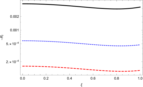
Figure 1: The ratio of the remainder contributions to the energy relative to the lowest order approximant, $R_{l}/E^{(2)}$ for isorefractive dielectric-diamagnetic balls. Plotted are the negative of this ratio for $l=1$ (solid, black), $l=2$ (dotted, blue), and $l=3$ (dashed, red).

Since the corrections are so small, for all $\xi$ the lowest UAE contribution is all that is discernable in a graph of the energy, Fig. 2.

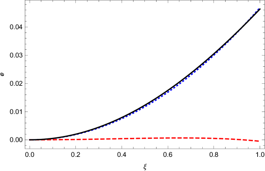
Figure 2: The energy for isorefractive dielectric-diamagnetic balls. Plotted are the first approximation (dotted, blue), the second approximation (dashed, red), and the total (solid, black).

Brevik and Kolbenstvedt Brevik (1982a) give an analytic approximant to the Casimir energy engineered to be exact for strong coupling $\xi=1$, but it does not give the exact low-$\xi$ behavior. The same is true for the approximation given in Brevik (1987). Brevik and Einevoll Brevik (1988) include dispersion in the coupling, but this leads to linearly divergent terms that are regulated by insertion of an arbitrary parameter. The direct mode sum given in Brevik (1998) includes the first three terms in the UAE, and is accurate to almost $0.1\%$, not quite so accurate as the results reported here.

III Dual Electromagnetic $\delta$ Sphere

In general, Casimir self energies of bodies are divergent, so it is of interest to study examples where unambiguous finite self energies can be extracted. Such is the case of a perfectly conducting spherical shell, or the diaphanous ball discussed in the previous section, which reduces to the former in the $\xi\to 1$ limit. Another generalization of the spherical shell that would seem to admit finiteness is an electromagnetic $\delta$-function sphere, with equal and opposite electric and magnetic couplings; it was observed in Parashar (2017) that then the catastrophic divergence in third-order in the coupling cancels, because only even powers in the coupling appear in the uniform asymptotic expansion of the energy integrand. It turns out, however, that this is a rather more subtle problem than we would have anticipated.

We follow the notation and formalism given in Parashar (2017). In this model, the couplings are modelled by a plasma-like dispersion relation, $\lambda_{e,g}=\zeta_{p,m}/\zeta^{2}$, and the form of the Casimir energy, after the bulk vacuum energy is subtracted, is [analogous to (3), except we have used a more general form of the frequency regulator]

$$E=-\frac{1}{4\pi}\sum_{l=1}^{\infty}(2l+1)P_{l}(\cos\delta)\int_{-\infty}^{\infty}d\zeta\frac{e^{i\zeta\tau}-1}{i\zeta\tau}\zeta\frac{d}{d\zeta}\ln\Delta^{E}\Delta^{H},$$ (12)

where the TE and TM modes are given by

$$\Delta^{E,H}=1+\zeta^{2}\frac{\lambda_{e}\lambda_{g}}{4}+|\zeta|[\lambda_{e,g}e_{l}(x)s_{l}(x)-\lambda_{g,e}e_{l}^{\prime}(x)s_{l}^{\prime}(x)],\quad x=|\zeta|a.$$ (13)

In Parashar (2017) we mostly considered the electric case where $\lambda_{g}=0$, but we did remark that interesting cancellations occur if $\lambda_{e}=-\lambda_{g}$. Here we will explore this further, and define $\lambda=\zeta_{p}a=-\zeta_{m}a$. This leads to the following form for the quantities in the logarithm:

$$\Delta^{E,H}=1-\frac{\lambda^{2}}{4x^{2}}\pm\frac{\lambda}{x}[e_{l}(x)s_{l}(x)+e_{l}^{\prime}(x)s_{l}^{\prime}(x)].$$ (14)

As we will see in Sec. III.4, there is a difficulty with this model, in that singularities appear for finite imaginary frequency $\zeta$ arising from the $e_{l}^{\prime}s_{l}^{\prime}$ terms.

III.1 Uniform Asymptotic Expansion

To focus on the ultraviolet behavior, we will modify the UAE expansions by replacing, as suggested in Parashar (2017), $1/z\to t$, which is correct for large $z$. Doing so leads to the modified UAE expansion (recall $x=\nu z$, $\nu=l+1/2$, $t=(1+z^{2})^{-1/2}$)

$$\ln\Delta^{E}\Delta^{H} \sim -\lambda^{2}\frac{t^{2}}{2\nu^{2}}-\lambda^{4}\frac{t^{4}}{16\nu^{4}}-\lambda^{2}\frac{t^{6}}{192\nu^{6}}[3(1-6t^{2}+6t^{4})^{2}+2\lambda^{4}]$$ (15)

$$\quad\mbox{}-\lambda^{2}\frac{t^{8}}{512\nu^{8}}[2(-1+t)(1+t)(1-6t^{2}+6t^{4})(-13+275t^{2}-840t^{4}+630t^{6})$$

$$\quad\mbox{}+4\lambda^{2}(1-6t^{2}+6t^{4})^{2}+\lambda^{6}]+O(\nu^{-10}).$$

In Parashar (2017) we did calculate the energies corresponding to the first two terms in this uniform expansion, just twice those from the $\lambda_{e}$ contribution. The $O(\nu^{-2})$ term in the UAE is in general sensitive to the regulator,

$$E^{(2)}=\frac{\lambda^{2}}{4a}\left(1-\frac{1}{\Delta}\right),$$ (16)

where $\Delta=\sqrt{\delta^{2}+\tilde{\tau}^{2}}$. The divergent term arises from the form of the temporal point splitting in Eq. (12). Had we used a simple imaginary exponential instead, and set $\delta=0$, no divergence would have appeared, as we saw in (6). However, the form of the divergence is that expected on general grounds, but it would seem it can be consistently removed. The fourth-order term is finite, but was not explicitly given in Parashar (2017). It is twice the $O(\lambda^{4})$ term evaluated in Eq. (4.14) in Milton:2017ghh :

$$E^{(4)}=-\frac{\lambda^{4}}{16a}\left(\frac{\pi^{2}}{8}-1\right).$$ (17)

III.2 First Approximation

Before we consider the general situation, let us see if we can extract some sort of reasonable approximation to the energy. We note that the leading terms in Eq. (15) (the highest power of $\lambda$ in each order of $1/\nu$) can be readily summed:

$$\ln\Delta^{E}\Delta^{H}\sim-2\sum_{n=1}^{\infty}\frac{1}{n}\left(\frac{\lambda t}{2\nu}\right)^{2n}=2\ln\left(1-\frac{\lambda^{2}t^{2}}{(2\nu)^{2}}\right).$$ (18)

The terms we have summed here might be presumed to be the largest contributions, since for a given power of $\lambda^{2}$, only the leading power of $1/\nu^{2}$ is kept. Then, if we subtract off the leading, divergent term, we can write this contribution to the energy as

$$\tilde{E}=E^{(2)}+\tilde{E}_{R},$$ (19)

where

$$E_{R}=-\frac{\lambda^{2}}{\pi a}\sum_{l=1}^{\infty}f(2\nu/\lambda),$$ (20)

in terms of the function

$$f(x)=\int_{0}^{1}dt\,t^{2}\sqrt{1-t^{2}}\frac{1}{x^{2}-t^{2}}=-\frac{\pi}{4}(1-2x^{2}+2x\sqrt{x^{2}-1}),$$ (21)

which only exists if $x>1$. For large $x$,

$$f(x)\sim\frac{\pi}{16x^{2}},\quad x\gg 1.$$ (22)

To improve convergence of the $l$ sum, we can subtract the next term in the UAE, so

$$\tilde{E}=E^{(2)}+E^{(4)}-\frac{\lambda^{2}}{\pi a}\sum_{l=1}^{\infty}\left[f\left(\frac{2\nu}{\lambda}\right)-\frac{\pi}{16}\left(\frac{\lambda}{2\nu}\right)^{2}\right].$$ (23)

From this, we can readily obtain a numerical estimate, based on this leading approximation, valid for $\lambda<3$, shown in Fig. 3.

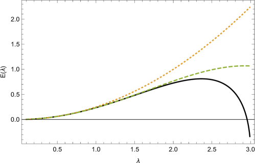
Figure 3: Energy estimate $\tilde{E}$ for a diaphanous ball (in units of $1/a$) based on the leading terms in the UAE as a function of the coupling $\lambda$. Plotted is the exact approximant (solid curve), the contribution of the leading order $E^{(2)}$ (with the $1/\Delta$ divergence removed) (dotted curve), and the sum of the first two leading orders $E^{(2)}+E^{(4)}$ (dashed curve). Although the exact approximant is finite at $\lambda=3$, it possesses infinite slope there, having changed sign for a slightly smaller value of $\lambda$.

The figure shows the first two UAE contributions, and the sum of all the leading terms as explained above, with the second-order divergence removed. It is to be noted that the exact approximant is finite at at $\lambda=3$, $\tilde{E}(\lambda=3)=-0.686434/a$, but it is singular there, since the derivative becomes infinite at that point. Therefore, it is unclear how to analytically continue this approximant result to higher values of the coupling $\lambda$.

III.3 $O(\lambda^{2})$ Contribution

We can also, in principle, compute the exact order-$\lambda^{2}$ contribution by doing the angular momentum sum exactly again using the addition theorem Klich:1999df . Indeed, the $l$-sum over the Bessel functions can be thus replaced by integrals over $w=2x\sqrt{2(1-\cos\delta)}$, for example,

$$\sum_{l=0}^{\infty}(2l+1)e_{l}^{2}(x)s_{l}^{2}(x)=\frac{x^{2}}{2}\int_{0}^{4x}\frac{dw}{w}e^{-w}.$$ (24)

The divergence at $w=0$ here is irrelevant because of the derivative appearing in Eq. (12). However, the terms involving derivatives of Bessel functions possess serious singularities when $\cos\delta=1$, which at present we do not see how to deal with. Although these structures represent the infrared singularities of the derivatives of the modified Bessel function, because they result in divergences when the field-points overlap, they seem to represent ultraviolet singularities not captured by the UAE.

III.4 General Analysis

The difficulties we have encountered in $O(\lambda^{2})$ are symptomatic of a more general pathology. It is easy to see that $\Delta^{E}$ always has one zero for finite positive $x$, and if $\lambda$ is large enough $\Delta^{H}$ does as well. (For $l=1$, the minimum value of $\lambda$ for $\Delta^{H}$ to develop a zero is $\lambda_{1}=8/3=2.666\dots$.) For large $\lambda$ both zeroes approach $\lambda/2$, as shown in Fig. 4.

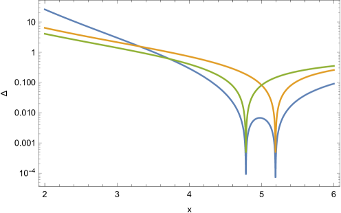
Figure 4: Zeroes of $\Delta^{E}$ (right) and $\Delta^{H}$ (left), and of their product, shown by the plots of their magnitudes, for $l=1$ and $\lambda=10$. As $\lambda$ gets large, the zeroes approach $\lambda/2$ for all $l$.

These zeroes translate into poles in the frequency integrand in (12). This is rather surprising, since the whole point of doing the Euclidean rotation of the frequency to the imaginary axis, $\omega\to i\zeta$, is to avoid singularities along the real axis. However, this phenomenon by itself is not fatal, since we would think the energy would be obtained by taking the real part of the expression (12), (14), that is, the principal values coming from these simple poles. But, numerically this is a bit challenging.

Therefore, a better scheme would seem to be to rotate back through $-\pi/4$, to a path of integration bisecting the first quadrant of the complex frequency plane. Removing the first two approximants coming from the UAE, we then obtain the following expression, which would seem amenable to numerical evaluation:

$$E=E^{(2)}+E^{(4)}-\frac{1}{4\pi a}\sum_{l=1}^{\infty}(2l+1)R_{l}(\lambda),$$ (25)

where the remainder is given by (the cutoff has been dropped, in the expectation that the remainder is finite)

$$R_{l}=\int_{0}^{\infty}dx\,w_{l}(x,\lambda),\quad w_{l}(x,\lambda)=\Re(1-i)x\frac{d}{dx}\left[\ln\Delta^{E}\Delta^{h}+\frac{\lambda^{2}t^{2}}{2\nu^{2}}+\frac{\lambda^{4}t^{4}}{(2\nu)^{2}}\right]_{x\to x(1-i)}.$$ (26)

The integrand, computed numerically, is plotted in Fig. 5.

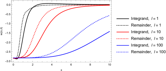
Figure 5: The integrand of the energy $w_{l}(x,\lambda)$ given by (26) for $\lambda=1$ and $l=1,10,100$, shown by the dotted lines. The solid lines show the unsubtracted $\ln\Delta^{E}\Delta^{H}$ integrand. The removal of the leading UAE contributions greatly improves the large $x$ behavior, but leaves large and growing contributions for moderate values of $x$.

It is seen that subtraction of the leading UAE contributions greatly suppresses the large $x$ behavior, so the integrals are rapidly convergent. However, because of the small $x$ singularities of the derivatives of the Bessel functions, there is a finite contribution at moderate $x$, all the way down to $x=0$, which grows with $l$. Consequently, when this is integrated over $x$, the remainder $R_{l}$ grows with $l$. This growth appears to be cubic. When the $P_{l}(\cos\delta)$ convergence factor is inserted into the $l$ summation, this would translate into a divergence going like $\delta^{-5}$, a quintic divergence. So we conclude that the UAE does not capture the real divergence of the self energy for the isorefractive sphere. Because of numerical errors, and the likely appearance of a subleading logarithmic divergence, it appears unfeasible to extract a finite remainder, even if the divergent terms can be “renormalized” away.

IV Conclusions

We have re-examined two situations which extend the classic problem of the ideal perfectly conducting sphere: the diaphanous dielectric-diamagnetic ball, where the speed of light is the same on both sides of the spherical surface, and the isorefractive $\delta$-function sphere, where the electric and magnetic couplings are equal and opposite. The former situation has been well studied, and is uniquely finite; here we extend the accuracy of the numerical calculations a bit. The latter situation, although apparently ultravioletly finite, possesses infrared sensitivity that translates into much more severe ultraviolet divergences than revealed by the UAE, which seem to make it practically impossible to extract a well-defined self energy. This sensitivity manifests itself as poles on the imaginary frequency axis in the energy integrand. By truncating the theory, We are able to make some estimates for small coupling $\lambda$. Further study of this suprisingly pathological model is warranted.