Strong convergence of a stochastic Rosenbrock-type scheme for the finite element discretization of semilinear SPDEs driven by multiplicative and additive noise

Abstract

This paper aims to investigate the numerical approximation of a general second order parabolic stochastic partial differential equation(SPDE) driven by multiplicative and additive noise. Our main interest is on such SPDEs where the nonlinear part is stronger than the linear part, usually called stochastic dominated transport equations. Most standard numerical schemes lose their good stability properties on such equations, including the current linear implicit Euler method. We discretize the SPDE in space by the finite element method and propose a novel scheme called stochastic Rosenbrock-type scheme for temporal discretization. Our scheme is based on the local linearisation of the semi-discrete problem obtained after space discretization and is more appropriate for such equations. We provide a strong convergence of the new fully discrete scheme toward the exact solution for multiplicative and additive noise and obtained optimal rates of convergence. Numerical experiments to sustain our theoretical results are provided.

1 Introduction

We consider the numerical approximation of the following SPDE

$$dX(t)+[AX(t)+F(X(t))]dt=B(X(t))dW(t),\quad X(0)=X_{0},\quad t\in(0,T],$$ (1)

in the Hilbert space $L^{2}(\Lambda)$, where $\Lambda\subset\mathbb{R}^{d}$, $d=1,2,3$ is bounded with smooth boundary, $T>0$ is the final time, $F$ and $B$ are nonlinear functions, $X_{0}$ is the initial data which is random and $A$ is a linear operator, unbounded, not necessary self-adjoint. Precise assumptions on $F$, $B$, $X_{0}$ and $A$ will be given in the next section. Equations of type (1) are used to model many real world phenomena in different fields such as biology, chemistry, physics [28, 3, 31, 29]. In many cases explicit solutions of SPDEs are unknown, therefore numerical approximations are powerful tools to provide realistic approximations. Numerical approximation of SPDE (1) is therefore an active research area and has attracted a lot of attentions since two decades (see e.g. [16, 34, 35, 12, 8, 9, 37, 36, 28, 26, 11]). Due to the time step restriction of the explicit Euler method, linear implicit Euler method is used in many situations. Linear implicit Euler method has been largely investigated in the literature (see e.g. [12, 35, 17, 33] and the references therein). The resolvent operator $(\mathbf{I}+\Delta tA_{h})^{-1}$ plays a key role to stabilise the linear implicit Euler method, where $A_{h}$ is the discrete version of $A$, obtained after the space discretization. Such approach is justified when the linear operator $A$ is strong. Indeed, when $A$ is stronger than $F$, the linear operator $A$ drives the SPDE (1) and the good stability properties of the linear implicit Euler method and exponential integrators are guaranteed. In more concrete applications, the nonlinear function $F$ can be stronger. Typical examples are stochastic reaction equations with stiff reaction term. For such equations, both linear implicit Euler method [12, 35, 17, 33] and exponential integrators [16, 34, 8] behave like the standard explicit Euler method (see Section 2.3) and therefore lose their good stabilities properties. For such problems in the deterministic context, exponential Rosenbrock-type methods [32, 7] and Rosenbrock-type methods [32, 21, 22] were proved to be efficient. Recently, the exponential Rosenbrock method was extended to the case of stochastic partial differential equations [19] and was proved to be very stable for stochastic reactive dominated transport equations. However the computation of the stochastic exponential matrix functions involve was far to be efficient. Since solving linear systems are more straightforward than computing the exponential of a matrix, it is important to develop alternative methods based on the resolution of linear systems, which may be more efficient if the appropriate preconditionners are used. In this paper, we propose a novel scheme based on the combination of the Rosenbrock-type method and the linear implicit Euler method. The resulting numerical scheme that we call stochastic Rosenbrock-type scheme(SROS) is stable and efficient in contrast to the exponential scheme in [19], which is only stable. The space discretization is performed using the finite element method and our novel scheme is based on the local linearization of the nonlinear drift part of the semi-discrete problem obtained after spatial discretization. The local linearization therefore weakens the nonlinear part of the drift function so that the linearized semi-disrete problem is driven by its new linear part, which changes at each time step. The standard linear implicit Euler method [12, 35] is then applied to the linearized semi-discrete problem. This combination yields our novel SROS scheme. We analyze the strong convergence of the novel fully discrete scheme toward the exact solution in the root-mean-square $L^{2}$-norm. The main challenge here comes from the fact that the resolvent operator $S^{m}_{h,\Delta t}(\omega)$ appearing in the numerical scheme (35) is not constant as it changes at each time step. Furthermore the operator $S^{m}_{h,\Delta t}(\omega)$ is a random operator. To address those challenges, we provide in Section 3.1 novel stability estimates to handle the composition of the perturbed random resolvent operators, useful in our convergence analysis. The results indicate how the convergence orders depend on the regularity of the initial data and the noise. More precisely, we achieve the optimal convergence orders $\mathcal{O}\left(h^{\beta}+\Delta t^{\frac{\min(\beta,1)}{2}}\right)$ for multiplicative noise and the optimal convergence orders $\mathcal{O}\left(h^{\beta}+\Delta t^{\frac{\beta}{2}-\epsilon}\right)$ for additive noise, where $\beta$ is the regularity’s parameter of the noise (see Assumption 2.2) and $\epsilon>0$ is an arbitrary number small enough.

The rest of this paper is organized as follows. Section 2 deals with the well posedness problem, the numerical scheme and the main results. In Section 3, we provide some error estimates for the deterministic homogeneous problem as preparatory results along with proof of the main results. Section 4 provides some numerical experiments to sustain the theoretical findings. Those numerical experiments show the efficiency of the novel scheme comparing to the exponential scheme developed in [19].

2 Mathematical setting and main results

2.1 Main assumptions and well posedness problem

Let us define functional spaces, norms and notations that will be used in the rest of the paper. Let $\left(H,\langle.,.\rangle_{H},\|.\|\right)$ be a separable Hilbert space. For all $p\geq 2$ and for a Banach space $U$, we denote by $L^{p}(\Omega,U)$ the Banach space of all equivalence classes of $p$ integrable $U$-valued random variables. We denote by $L(U,H)$ the space of bounded linear mappings from $U$ to $H$ endowed with the usual operator norm $\|.\|_{L(U,H)}$. By $\mathcal{L}_{2}(U,H):=HS(U,H)$, we denote the space of Hilbert-Schmidt operators from $U$ to $H$. We equip $\mathcal{L}_{2}(U,H)$ with the norm

$$\|l\|^{2}_{\mathcal{L}_{2}(U,H)}:=\sum_{i=1}^{\infty}\|l\psi_{i}\|^{2},\quad l\in\mathcal{L}_{2}(U,H),$$ (2)

where $(\psi_{i})_{i=1}^{\infty}$ is an orthonormal basis of $U$. Note that (2) is independent of the orthonormal basis of $U$. For simplicity, we use the notations $L(U,U)=:L(U)$ and $\mathcal{L}_{2}(U,U)=:\mathcal{L}_{2}(U)$. It is well known that for all $l\in L(U,H)$ and $l_{1}\in\mathcal{L}_{2}(U)$, $ll_{1}\in\mathcal{L}_{2}(U,H)$ and

$$\|ll_{1}\|_{\mathcal{L}_{2}(U,H)}\leq\|l\|_{L(U,H)}\|l_{1}\|_{\mathcal{L}_{2}(U)}.$$ (3)

In the rest of this paper, we take $H=L^{2}(\Lambda)$. In order to ensure the existence and the uniqueness of the solution of (1), and for the purpose of the convergence analysis, we make the following assumptions.

Assumption 2.1

[Linear operator $A$] $-A:\mathcal{D}(A)\subset H\longrightarrow H$ is the generator of an analytic semigroup $S(t)=:e^{-At}$ on $L^{2}(\Lambda)$, i.e. $S(t)$ is given as follows [6, 24, 1, 2]

$$S(t)=\frac{1}{2\pi i}\int_{\mathcal{C}}e^{-t\lambda}(\lambda\mathbf{I}-A)^{-1}d\lambda,\quad t>0,$$

where $\mathcal{C}$ denotes a path that surrounds the spectrum of $-A$.

Assumption 2.2

[Initial value $X_{0}$] The initial value $X_{0}$ belongs to $L^{p}\left(\Omega,\mathcal{D}\left((A)^{\frac{\beta}{2}}\right)\right)$, for some $\beta\in(0,2]$ and some $p\in[2,\infty)$.

As in the current literature for deterministic Rosenbrock-type methods [22, 21], deterministic exponential Rosemnbrock-type method [7, 20] and stochastic exponential Rosenbrock-type methods [19], we make the following assumption on the nonlinear drift term.

Assumption 2.3

[Nonlinear term $F$] The nonlinear map $F:H\longrightarrow H$ is Fréchet differentiable with bounded derivative, i.e. there exists a constant $b>0$ such that

$$\|F^{\prime}(u)\|_{L(H)}\leq b,\quad u\in H.$$ (4)

Moreover, as in [14, Page 6] for deterministic Rosenbrock-type method, we assume that the resolvent set of $-A-F^{\prime}(u)$ contains $(0,\infty)$ for all $u\in H$.

Remark 2.1

Inequality (4) together with the mean value theorem show that there exists a constant $C_{F}=C_{F}(b)\geq 0$ such that

$$\|F(u)-F(v)\|\leq C_{F}\|u-v\|,\quad u,v\in H.$$ (5)

In addition, if $\|F(0)\|<\infty$, then from (5) there exists a constant $C=(C_{F},\|F(0)\|)\geq 0$ such that

$$\|F(u)\|\leq\|F(0)\|+\|F(u)-F(0)\|\leq\|F(0)\|+C_{F}\|u\|\leq C(1+\|u\|),\quad u\in H.$$

Remark 2.2

An illustrative example for which the resolvent set of $-A-F^{\prime}(u)$ contains $(0,\infty)$ is obtained when $A$ generates a contraction semigroup and the derivative of the nonlinear drift term $F$ satisfies the following coercivity condition

$$\left\langle F^{\prime}(u)v,v\right\rangle_{H}\geq 0,\quad u,v\in H.$$ (6)

In fact, it follows from (6) that $-F^{\prime}(u)$ is an relatively $A$-bounded and dissipative operator with $A$-bound $a_{0}=0$ (see e.g. [1, Chapter III, Definition 2.1]). Therefore, from [1, Chapter III, Theorem 2.7], it follows that $-A-F^{\prime}(u)$ is a generator of a contraction semigroup. Hence, for all $u\in H$ $(0,\infty)\subset\rho\left(-A-F^{\prime}(u)\right)$.

Remark 2.3

The condition $(0,\infty)\subset\rho\left(-A-F^{\prime}(u)\right)$ on Assumption 2.3 can be relaxed, but the drawback is that the resolvent set of the perturbed semigroup is smaller than that of the initial semigroup.

Let $\left(\Omega,\mathcal{F},\mathbb{P}\right)$ be a probability space and $\{\mathcal{F}_{t}\}_{t\in[0,T]}$ a normal filtration on $\left(\Omega,\mathcal{F},\mathbb{P}\right)$, that is $\{\mathcal{F}_{t}\}_{t\in[0,T]}$ is a filtration on $\left(\Omega,\mathcal{F},\mathbb{P}\right)$ satisfying the following (see e.g. [27, Definition 2.1.11]):

• $\mathcal{F}_{0}$ contains all elements $O\in\mathcal{F}$ with $\mathbb{P}(O)=0$,

• $\mathcal{F}_{t}=\mathcal{F}_{t^{+}}:=\bigcap\limits_{s>t}\mathcal{F}_{s}$ for all $t\in[0,T]$.

Let $Q:H\longrightarrow H$ be a linear selfadjoint and positive operator. In this work, the noise $W(t)=W(x,t)$ is assumed to be an $H$-valued $Q$-Wiener process defined in the filtered probability space $\left(\Omega,\mathcal{F},\mathbb{P},\{\mathcal{F}_{t}\}_{t\geq 0}\right)$. Let us recall below the definition of a $Q$-Wiener process.

Definition 2.1

[$Q$-Wiener process][27, Definition 2.1.12]. An $H$-valued stochastic process $\{W(t):t\geq 0\}$ is called $Q$-Wiener process if

1. $W(0)=0$ almost surely (a.s).

2. The application $t\longmapsto W(t,\omega)$ is continuous from $\mathbb{R}^{+}$ to $H$ for every $\omega\in\Omega$.

3. $W(t)$ is $\mathcal{F}_{t}$-adapted and $W(t)-W(s)$ is independent of $\mathcal{F}_{s}$ for $s<t$.

4. For all $0\leq s\leq t$, the random variable $W(t)-W(s)$ follows a normal distribution with mean $0$ and covariance operator $(t-s)Q$. We write $W(t)-W(s)\sim\mathcal{N}\left(0,(t-s)Q\right)$.

It is well known that if $Q$ has finite trace , then the $Q$-Wiener process $W(t)$ can be represented as follows [27, Proposition 2.1.10]

$$W(x,t)=\sum_{i\in\mathbb{N}}\sqrt{q_{i}}e_{i}(x)\beta_{i}(t),\quad t\in[0,T],\quad x\in\Lambda,$$ (7)

where $q_{i}$, $e_{i}$, $i\in\mathbb{N}$ are respectively the eigenvalues and the eigenfunctions of the covariance operator $Q$, and $\beta_{i}$ are independent and identically distributed standard Brownian motions.

The space of Hilbert-Schmidt operators from $Q^{\frac{1}{2}}(H)$ to $H$ is denoted by $L^{0}_{2}=\mathcal{L}_{2}(Q^{\frac{1}{2}}(H),H)=:HS(Q^{\frac{1}{2}}(H),H)$ with the corresponding norm $\|.\|_{L^{0}_{2}}$ defined by

$$\|l\|_{L^{0}_{2}}:=\|lQ^{\frac{1}{2}}\|_{HS}=\left(\sum_{i=1}^{\infty}\|lQ^{\frac{1}{2}}e_{i}\|^{2}\right)^{\frac{1}{2}},\quad l\in L^{0}_{2},$$ (8)

where $(e_{i})_{i=1}^{\infty}$ is an orthonormal basis of $H$. Note that (8) is also independent of the orthonormal basis of $H$. Following [25, Chapter 7] or [36, 16, 10, 12], we make the following assumption on the diffusion term.

Assumption 2.4

[Diffusion term ] The operator $B:H\longrightarrow L^{0}_{2}$ satisfies the global Lipschitz condition, i.e. there exists a positive constant $C_{B}$ such that

$$\|B(0)\|_{L^{0}_{2}}\leq C_{B},\quad\|B(u)-B(v)\|_{L_{2}^{0}}\leq C_{B}\|u-v\|,\quad u,v\in H.$$

As a consequence of Assumption 2.4, it holds that

$$\|B(u)\|_{L^{0}_{2}}\leq\|B(0)\|_{L^{0}_{2}}+\|B(u)-B(0)\|_{L^{0}_{2}}\leq\|B(0)\|_{L^{0}_{2}}+C_{B}\|u\|\leq C_{B}(1+\|u\|),\quad u\in H.$$

We equip $V_{\alpha}:=\mathcal{D}(A^{\frac{\alpha}{2}})$, $\alpha\in\mathbb{R}$ with the norm $\|v\|_{\alpha}:=\|A^{\frac{\alpha}{2}}v\|$, for all $v\in V_{\alpha}$. It is well known that $(V_{\alpha},\|.\|_{\alpha})$ is a Banach space [6].

To establish our root-mean-square $L^{2}$ strong convergence result when dealing with multiplicative noise, we will also need the following further assumption on the diffusion term when $\beta\in[1,2)$, which was also used in [10, 13] to achieve optimal regularity rates in space and time, and in [16, 12, 19] to achieve optimal strong convergence rates.

Assumption 2.5

There exists a positive constant $c\geq 0$ such that

$$B\left(\mathcal{D}\left(A^{\frac{(\beta-1)}{2}}\right)\right)\subset HS\left(Q^{\frac{1}{2}}(H),\mathcal{D}\left(A^{\frac{(\beta-1)}{2}}\right)\right)\;\text{and}\;\left\|A^{\frac{(\beta-1)}{2}}B(v)\right\|_{L^{0}_{2}}\leq c\left(1+\|v\|_{\beta-1}\right)$$

for all $v\in\mathcal{D}\left(A^{\frac{(\beta-1)}{2}}\right)$, where $\beta$ comes from Assumption 2.2.

Typical examples fulfilling Assumption 2.5 are stochastic reaction diffusion equations (see e.g. [10, Section 4]).

When dealing with additive noise (i.e. when $B=\mathbf{I}$), the strong convergence proof will make use of the following assumption, also used in [35, 34, 19].

Assumption 2.6

The covariance operator $Q$ satisfies the following estimate

$$\left\|A^{\frac{\beta-1}{2}}Q^{\frac{1}{2}}\right\|_{\mathcal{L}_{2}(H)}\leq C_{Q},$$ (9)

where $\beta$ comes from Assumption 2.2 and $C_{Q}$ is a positive constant.

When dealing with additive noise, to achieve convergence order greater than $\frac{1}{2}$ in time, we use the following further assumption on the nonlinear function, also used in [34, 35, 19].

Assumption 2.7

The deterministic mapping $F:H\longrightarrow H$ is twice differentiable and there exist two constants $L\geq 0$ and $\eta\in(0,2)$ such that

$$\|F^{\prime}(u)v\|\leq L\|v\|,\quad\|F^{\prime\prime}(u)(v_{1},v_{2})\|_{-\eta}\leq L\|v_{1}\|.\|v_{2}\|,\quad u,v,v_{1},v_{2}\in H.$$

The following proposition will be useful in the rest of the paper.

Proposition 2.1

[Smoothing properties of the semigroup][6] Let $\alpha>0$, $\delta\geq 0$ and $0\leq\gamma\leq 1$, then there exists a constant $C>0$ such that

$$\|A^{\delta}S(t)\|_{L(H)}\leq Ct^{-\delta},\quad t>0;\quad\|A^{-\gamma}\left(\mathbf{I}-S(t)\right)\|_{L(H)}\leq Ct^{\gamma},\quad t\geq 0;$$

$$A^{\delta}S(t)=S(t)A^{\delta}\quad\text{on}\quad\mathcal{D}(A^{\delta})\quad\text{and}\quad\|D^{l}_{t}S(t)v\|_{\delta}\leq Ct^{-l-\frac{(\delta-\alpha)}{2}}\|v\|_{\alpha},\quad t>0,\quad v\in\mathcal{D}(A^{\frac{\alpha}{2}});$$

where $l=0,1$, and $D^{l}_{t}=\dfrac{d^{l}}{dt^{l}}$. Moreover, if $\delta\geq\gamma$ then $\mathcal{D}(A^{\delta})\subset\mathcal{D}(A^{\gamma})$.

The well posedness result is given in the following theorem.

Theorem 2.1

[25, Theorem 7.2]
Let Assumptions 2.1, 2.3 and 2.4 be satisfied. If $X_{0}$ is a $\mathcal{F}_{0}$-measurable $H$-valued random variable, then there exists a unique mild solution $X$ of (1), which has the following representation

$$X(t)=S(t)X_{0}-\int_{0}^{t}S(t-s)F(X(s))ds+\int_{0}^{t}S(t-s)B(X(s))dW(s),\quad t\in(0,T]$$ (10)

and satisfies

$$\mathbb{P}\left[\int_{0}^{T}\|X(s)\|^{2}ds<\infty\right]=1.$$

Moreover, for any $p\geq 2$, there exists a constant $C=C(p,T)>0$ such that

$$\sup_{t\in[0,T]}\mathbb{E}\|X(t)\|^{p}\leq C(1+\mathbb{E}\|X_{0}\|^{p}).$$

2.2 Finite element discretization

In the rest of the paper, to simplify the presentation, we consider the linear operator $A$ to be of second-order. More precisely, we consider the SPDE (1) to be a second-order semilinear parabolic SPDE of the following form

$$dX(t,x)+[-\nabla\cdot\left(\mathbf{D}\nabla X(t,x)\right)+\mathbf{q}\cdot\nabla X(t,x)]dt+f(x,X(t,x))dt=b(x,X(t,x))dW(t,x),$$ (11)

for $x\in\Lambda$ and $t\in(0,T]$, where the functions $f:\Lambda\times\mathbb{R}\longrightarrow\mathbb{R}$ and $b:\Lambda\times\mathbb{R}\longrightarrow\mathbb{R}$ are continuously differentiable with globally bounded derivatives. In the abstract framework (1), the linear operator $A$ is the $L^{2}(\Lambda)$ realization [2, p. 812] of the following differential operator

$$\mathcal{A}u=-\sum_{i,j=1}^{d}\dfrac{\partial}{\partial x_{i}}\left(D_{ij}(x)\dfrac{\partial u}{\partial x_{j}}\right)+\sum_{i=1}^{d}q_{i}(x)\dfrac{\partial u}{\partial x_{i}},\quad\mathbf{D}:=\left(D_{i,j}\right)_{1\leq i,j\leq d},\quad\mathbf{q}:=\left(q_{i}\right)_{1\leq i\leq d}.$$ (12)

where $D_{ij}\in L^{\infty}(\Lambda)$, $q_{i}\in L^{\infty}(\Lambda)$ and there exists a constant $c_{1}>0$ such that

$$\sum_{i,j=1}^{d}D_{ij}(x)\xi_{i}\xi_{j}\geq c_{1}|\xi|^{2},\quad\xi\in\mathbb{R}^{d},\quad x\in\overline{\Lambda}.$$

The functions $F:H\longrightarrow H$ and $B:H\longrightarrow HS\left(Q^{\frac{1}{2}}(H),H\right)$ are defined respectively by

$$\left(F(v)\right)(x)=f\left(x,v(x)\right),\quad\left(B(v)u\right)(x)=b\left(x,v(x)\right).u(x),\quad x\in\Lambda,\;v\in H,\;u\in Q^{\frac{1}{2}}(H).$$ (13)

For an appropriate family of eigenfunctions $(e_{i})_{i\in\mathbb{N}}$ such that $\sup\limits_{i\in\mathbb{N}^{d}}\left[\sup\limits_{x\in\Lambda}\|e_{i}(x)\|\right]<\infty$, it is well known that the Nemystskii operator $F$ related to $f$ and the multiplication operator $B$ associated to the function $b$ defined in (13) satisfy Assumptions 2.3, 2.4 and 2.5, see e.g. [10, Section 4]. As in [16, 2] we introduce two spaces $\mathbb{H}$ and $V$, such that $\mathbb{H}\subset V$; the two spaces depend on the boundary conditions and the domain of the operator $A$. For Dirichlet (or first-type) boundary conditions we take

$$V=\mathbb{H}=H^{1}_{0}(\Lambda)=\{v\in H^{1}(\Lambda):v=0\quad\text{on}\quad\partial\Lambda\}.$$

For Robin (third-type) boundary condition and Neumann (second-type) boundary condition, which is a special case of Robin boundary condition, we take $V=H^{1}(\Lambda)$

$$\mathbb{H}=\{v\in H^{2}(\Lambda):\partial v/\partial\mathtt{v}_{\mathcal{A}}+\alpha_{0}v=0,\quad\text{on}\quad\partial\Lambda\},\quad\alpha_{0}\in\mathbb{R},$$

where $\partial v/\partial\mathtt{v}_{\mathcal{A}}$ is the normal derivative of $v$ and $\mathtt{v}_{A}$ is the exterior pointing normal at $n=(n_{i})$ to the boundary of $\mathcal{A}$, given by

$$\partial v/\partial\mathtt{v}_{\mathcal{A}}=\sum_{i,j=1}^{d}n_{i}(x)D_{ij}(x)\dfrac{\partial v}{\partial x_{j}},\qquad x\in\partial\Lambda.$$

Using Green’s formula and the boundary conditions, the corresponding bilinear form associated to $\mathcal{A}$ and $A$ is given by

$$a(u,v)=\int_{\Lambda}\left(\sum_{i,j=1}^{d}D_{ij}\dfrac{\partial u}{\partial x_{i}}\dfrac{\partial v}{\partial x_{j}}+\sum_{i=1}^{d}q_{i}\dfrac{\partial u}{\partial x_{i}}v\right)dx,\quad u,v\in V,$$

for Dirichlet and Neumann boundary conditions, and

$$a(u,v)=\int_{\Lambda}\left(\sum_{i,j=1}^{d}D_{ij}\dfrac{\partial u}{\partial x_{i}}\dfrac{\partial v}{\partial x_{j}}+\sum_{i=1}^{d}q_{i}\dfrac{\partial u}{\partial x_{i}}v\right)dx+\int_{\partial\Lambda}\alpha_{0}uvdx,\quad u,v\in V,$$

for Robin boundary conditions. Using Gårding’s inequality (see e.g. [29]), it holds that there exist two constants $c_{0}$ and $\lambda_{0}>0$ such that

$$a(v,v)\geq\lambda_{0}\|v\|^{2}_{H^{1}(\Lambda)}-c_{0}\|v\|^{2},\quad v\in V.$$ (14)

By adding and substracting $c_{0}Xdt$ in both sides of (1), we have a new linear operator still denoted by $A$, and the corresponding bilinear form is also still denoted by $a$. Therefore, the following coercivity property holds

$$a(v,v)\geq\lambda_{0}\|v\|^{2}_{1},\quad v\in V.$$ (15)

Note that the expression of the nonlinear term $F$ has changed as we included the term $c_{0}X$ in the new nonlinear term that we still denote by $F$. The coercivity property (15) implies that $-A$ is sectorial on $L^{2}(\Lambda)$, i.e. there exist $C_{1},\,\theta\in(\frac{1}{2}\pi,\pi)$ such that

$$\|(\lambda I+A)^{-1}\|_{L(L^{2}(\Lambda))}\leq\dfrac{C_{1}}{|\lambda|},\;\quad\quad\lambda\in S_{\theta},$$

where $S_{\theta}:=\left\{\lambda\in\mathbb{C}:\lambda=\rho e^{i\phi},\;\rho>0,\;0\leq|\phi|\leq\theta\right\}$ (see e.g. [6]). The coercivity property (15) implies that $-A$ is the infinitesimal generator of a contraction semigroup $S(t)=e^{-tA}$ on $L^{2}(\Lambda)$. The coercivity property (15) also implies that $A$ is positive and its fractional powers are well defined for any $\alpha>0,$ by

$$\left\{\begin{array}[]{rcl}A^{-\alpha}&=&\frac{1}{\Gamma(\alpha)}\displaystyle\int_{0}^{\infty}t^{\alpha-1}{\rm e}^{-tA}dt,\\ A^{\alpha}&=&(A^{-\alpha})^{-1},\end{array}\right.$$ (16)

where $\Gamma(\alpha)$ is the Gamma function (see [6]). Let us now turn our attention to the space discretization of our problem (1). We start by splitting the domain $\Lambda$ in finite triangles. Let $\mathcal{T}_{h}$ be the triangulation with maximal length $h$ satisfying the usual regularity assumptions, and $V_{h}\subset V$ be the space of continuous functions that are piecewise linear over the triangulation $\mathcal{T}_{h}$. We consider the projection $P_{h}$ from $H=L^{2}(\Lambda)$ to $V_{h}$ defined for every $u\in H$ by

$$\langle P_{h}u,\chi\rangle_{H}=\langle u,\chi\rangle_{H},\quad\chi\in V_{h}.$$ (17)

The discrete operator $A_{h}:V_{h}\longrightarrow V_{h}$ is defined by

$$\langle A_{h}\phi,\chi\rangle_{H}=\langle A^{\frac{1}{2}}\phi,(A^{*})^{\frac{1}{2}}\chi\rangle_{H}=a(\phi,\chi),\quad\phi,\chi\in V_{h},$$ (18)

Like $-A$, $-A_{h}$ is also a generator of a bounded analytic semigroup $S_{h}(t)$ on $V_{h}$, given by (see e.g. [2, Chapter II, (7.14)] or [15])

$$S_{h}(t)=e^{-tA_{h}}=\frac{1}{2\pi i}\int_{\mathcal{C}}e^{-t\lambda}(\lambda\mathbf{I}-A_{h})^{-1}d\lambda,\quad t>0,$$

where $\mathcal{C}$ is a path that surrounds the spectrum of $-A_{h}$. Let $K$ be a constant satisfying

$$\|S_{h}(t)\|_{L(H)}\leq K,\quad t\geq 0.$$ (19)

As any semigroup and its generator, $-A_{h}$ and $S_{h}(t)$ satisfy the smoothing properties of Proposition 2.1 with a uniform constant $C$ (i.e. independent of $h$). Following [15, 16, 2], we characterize the domain of the operator $A^{\frac{\gamma}{2}},\,1\leq\gamma\leq 2$ as follows:

$$\mathcal{D}(A^{\frac{\gamma}{2}})=\mathbb{H}\cap H^{\gamma}(\Lambda)\;\text{ for Dirichlet boundary conditions},$$

$$\mathcal{D}(A)=\mathbb{H},\quad\mathcal{D}(A^{\frac{1}{2}})=H^{1}(\Lambda)\;\text{for Robin boundary conditions}.$$

The semi-discrete version of (1) consists to find $X^{h}(t)\in V_{h}$, $t\in(0,T]$ such that

$$dX^{h}(t)+[A_{h}X^{h}(t)+P_{h}F(X^{h}(t))]dt=P_{h}B(X^{h}(t))dW(t),\quad X^{h}(0)=P_{h}X_{0},\quad t\in(0,T].$$ (20)

The proof of the following lemma can be found in [19, Lemma 4 & Lemma 5]. Its provides the space and time regularities of the mild solution $X^{h}(t)$ of (20).

Lemma 2.1

• Let Assumptions 2.1 (with $\beta\in[0,1)$), 2.2, 2.3 and 2.4 be fulfilled. Then the mild solution $X^{h}(t)$ of (20) satisfies the following regularity estimates

  $$\left\|A_{h}^{\frac{\beta}{2}}X^{h}(t)\right\|_{L^{p}(\Omega,H)} \leq C\left(1+\left\|A^{\frac{\beta}{2}}X_{0}\right\|_{L^{p}(\Omega,H)}\right),\quad t\in[0,T],$$ (21)

  $$\left\|X^{h}(t_{2})-X^{h}(t_{1})\right\|_{L^{p}(\Omega,H)} \leq C|t_{2}-t_{1}|^{\frac{\beta}{2}}\left(1+\left\|A^{\frac{\beta}{2}}X_{0}\right\|_{L^{p}(\Omega,H)}\right),\;t_{1},t_{2}\in[0,T].$$ (22)

  Moreover, if $\beta\in[1,2)$ and if Assumption 2.5 is fulfilled, then

  $$\left\|X^{h}(t_{2})-X^{h}(t_{1})\right\|_{L^{p}(\Omega,H)} \leq C|t_{2}-t_{1}|^{\frac{1}{2}}\left(1+\left\|A^{\frac{\beta}{2}}X_{0}\right\|_{L^{p}(\Omega,H)}\right),\;t_{1},t_{2}\in[0,T].$$

• Let Assumptions 2.1, 2.2, 2.3 and 2.7 be fulfilled with $\beta\in[0,2)$. Then the mild solution $X^{h}(t)$ of (20) in the case of additive noise satisfies the following regularity estimates

  $$\left\|A_{h}^{\frac{\beta}{2}}X^{h}(t)\right\|_{L^{p}(\Omega,H)}\leq C\left(1+\left\|A^{\frac{\beta}{2}}X_{0}\right\|_{L^{p}(\Omega,H)}\right),\quad t\in[0,T],$$ (23)

  $$\left\|X^{h}(t_{2})-X^{h}(t_{1})\right\|_{L^{p}(\Omega,H)}\leq C|t_{2}-t_{1}|^{\frac{\min(\beta,1)}{2}}\left(1+\left\|A^{\frac{\beta}{2}}X_{0}\right\|_{L^{p}(\Omega,H)}\right),\;t_{1},t_{2}\in[0,T].$$ (24)

Here $C=C(C_{F},C_{B},C_{Q},\|F(0)\|,T,\beta)$ is a positive constant, independent of $h$, $t$, $t_{1}$ and $t_{2}$.

Corollary 2.1

As a consequence of Lemma 2.1, it holds that

$$\|X^{h}(t)\|_{L^{p}(\Omega,H)}\leq C,\quad\left\|F\left(X^{h}(t)\right)\right\|_{L^{p}(\Omega,H)}\leq C,\quad\left\|B\left(X^{h}(t)\right)\right\|_{L^{p}(\Omega,H)}\leq C,\quad t\in[0,T].$$

2.3 Standard linear implicit Euler method and stability properties

Let us recall that the linear implicit Euler scheme applied to the semi-discrete problem (30) is given by

$$Z^{h}_{m+1} = S_{h,\Delta t}Z^{h}_{m}+\Delta tS_{h,\Delta t}P_{h}F(Z^{h}_{m})+S_{h,\Delta t}P_{h}B(Z^{h}_{m}),$$ (25)

$$S_{h,\Delta t} := \left(\mathbf{I}+\Delta tA_{h}\right)^{-1},\quad Z^{h}_{0}=P_{h}X_{0}.$$ (26)

If the linear operator $A$ tends to the null operator, its corresponding discrete version $A_{h}$ tends to the null operator and $S_{h,\Delta t}$ tends to the identity operator $\mathbf{I}$. In this case, the numerical scheme (25) and the standard exponential integrator [16] behave like the unstable Euler-Maruyama scheme. See also [19, Section 2.3] for more details. For a simple illustration of the stability properties of such problems, let us consider the following deterministic linear differential equation

$$y^{\prime}=ay+cy,\quad a>0,c<0,\quad\text{such that}\quad c<-a.$$ (27)

The linear implicit Euler method applied to (27) by considering $F(y)=cy$ as the nonlinear part is given by

$$y_{n+1}=\frac{1+c\Delta t}{1-a\Delta t}y_{n},\quad n\geq 0.$$ (28)

The numerical scheme (28) is stable [32, 23] if and only if $\Delta t<\frac{2}{a-c}$. Note that when $a$ is small enough and $|c|$ large enough, the numerical scheme (28) behaves like the explicit Euler method and the stability region becomes very small. Rosenbrock-type methods were proved to be efficient in such situations and were studied in [5, 4, 23] for ordinary differential equations. Applying the Rosenbrock-Euler method to the linear problem (27) yields

$$y_{n+1}=\frac{1}{1-(a+c)\Delta t}y_{n},\quad n\geq 0.$$ (29)

Note that (29) coincides with the full implicit method with $F(y)=cy$. Rosenbrock-Euler method (29) is unconditionally stable (A-stable). This demonstrates the strong stability property of Rosenbrock-type methods for stiff problems. Authors of [21, 22] extended Rosenbrock-type methods to parabolic partial differential equations and the methods were proved to be efficient for solving transport equations in porous media [32]. To the best of our knowledge, the case of stiff stochastic partial differential equations is not yet studied in the scientific literature and will be the aim of this paper.

2.4 Novel fully discrete scheme and main results

Let us build a more stable scheme, robust when the linear operator $A$ tends to null operator. For the time discretization, we consider the one-step method which provides the numerical approximated solution $X^{h}_{m}$ of $X^{h}(t_{m})$ at discrete time $t_{m}=m\Delta t$, $m=0,\cdots,M$. The method is based on the continuous linearization of (20). More precisely, we linearize (20) at each time step as follows

$$dX^{h}(t)+[A_{h}X^{h}(t)+J_{m}^{h}X^{h}(t)]dt=G^{h}_{m}\left(X^{h}(t)\right)dt+P_{h}B\left(X^{h}(t)\right)dW(t),\;t_{m}\leq t\leq t_{m+1},$$ (30)

where $J_{m}^{h}$ is the Fréchet derivative of $P_{h}F$ at $X^{h}_{m}$ and $G^{h}_{m}$ is the remainder at $X^{h}_{m}$. Both $J^{h}_{m}$ and $G^{h}_{m}$ are random variables and are defined for all $\omega\in\Omega$ by

$$J^{h}_{m}(\omega) := (P_{h}F)^{\prime}(X^{h}_{m}(\omega))=P_{h}F^{\prime}(X^{h}_{m}(\omega)),$$ (31)

$$G^{h}_{m}(\omega)(X^{h}(t)) := -P_{h}F(X^{h}(t))+J_{m}^{h}(\omega)X^{h}(t).$$ (32)

Applying the linear implict Euler method to (30) yields the following fully discrete scheme, called stochastic Rosenbrock-type scheme (SROS)

$$\left\{\begin{array}[]{ll}X^{h}_{0}=P_{h}X_{0},\\ X^{h}_{m+1}=S^{m}_{h,\Delta t}X^{h}_{m}+\Delta tS^{m}_{h,\Delta t}G^{h}_{m}(X^{h}_{m})+S^{m}_{h,\Delta t}P_{h}B(X^{h}_{m})\Delta W_{m},\end{array}\right.$$ (35)

where $\Delta W_{m}$ and $S_{h,\Delta t}$ are defined respectively by

$$\Delta W_{m}:=W_{t_{m+1}}-W_{t_{m}},\quad\quad S^{m}_{h,\Delta t}(\omega):=\left(\mathbf{I}+\Delta tA_{h,m}(\omega)\right)^{-1},$$ (36)

and the linear operator $A_{h,m}$ is given by

$$A_{h,m}(\omega):=A_{h}+J^{h}_{m}(\omega),\quad\omega\in\Omega.$$ (37)

In the numerical scheme (35), the resolvent operator (defined in (36)) is random and changes at each time step. Having the numerical method (35) in hand, our goal is to analyze its strong convergence toward the exact solution in the root-mean-square $L^{2}$ norm for multiplicative and additive noise.

Throughout this paper we take $t_{m}=m\Delta t\in[0,T]$, where $\Delta t=\frac{T}{M}$ for $m,M\in\mathbb{N}$, $m\leq M$, $C$ is a generic constant that may change from one place to another but is independent of both $\Delta t$ and $h$. The main results of this paper are formulated in the following theorems.

Theorem 2.2

[Multiplicative noise] Let $X(t_{m})$ and $X^{h}_{m}$ be respectively the mild solution given by (10) and the numerical approximation given by (35) at $t_{m}=m\Delta t$. Let Assumptions 2.1, 2.2 (with $p=2$), 2.3 and 2.4 be fulfilled.

• If $0<\beta<1$, then the following error estimate holds

  $$\|X(t_{m})-X^{h}_{m}\|_{L^{2}(\Omega,H)}\leq C\left(h^{\beta}+\Delta t^{\frac{\beta}{2}}\right).$$

• If $1\leq\beta\leq 2$ and if Assumption 2.5 is fulfilled, then the following error estimate holds

  $$\|X(t_{m})-X^{h}_{m}\|_{L^{2}(\Omega,H)}\leq C\left(h^{\beta}+\Delta t^{\frac{1}{2}}\right),$$

where $C=C(C_{F},C_{B},T,\|F(0)\|,c,X_{0}))$ is a positive constant independent of $h$, $M$ and $\Delta t$.

Theorem 2.3

[Additive noise] When dealing with additive noise (i.e. when $B=\mathbf{I}$), let Assumptions 2.1, 2.2 with $p=4$, 2.3, 2.6 and 2.7 be fulfilled. Then the following error estimate holds for the mild solution $X(t)$ of (1) and the numerical approximation (35)

$$\|X(t_{m})-X^{h}_{m}\|_{L^{2}(\Omega,H)}\leq C\left(h^{\beta}+\Delta t^{\frac{\beta}{2}-\epsilon}\right),$$ (38)

where $C=C(C_{F},C_{Q},T,\|F(0)\|,X_{0})$ is a positive constant independent of $h$, $M$ and $\Delta t$.

3 Proof of the main results

The proofs of the main results require some preparatory results.

3.1 Preparatory results

For non commutative operators $H_{j}$ in a Banach space, we introduce the following notation, which will be used in the rest of the paper.

$$\prod_{j=l}^{k}H_{j}:=\left\{\begin{array}[]{ll}H_{k}H_{k-1}\cdots H_{l},\quad\text{if}\quad k\geq l,\\ \mathbf{I},\quad\hskip 68.28644pt\text{if}\quad k<l.\end{array}\right.$$

Lemma 3.1

[19, Lemma 10] Let Assumption 2.2 be fulfilled. Then for all $\omega\in\Omega$ the following estimate holds

$$\left\|\left(\prod_{j=l}^{m}e^{\Delta tA_{h,j}(\omega)}\right)A_{h}^{\gamma}\right\|_{L(H)}\leq Ct_{m+1-l}^{-\gamma},\quad 0\leq l\leq m,\quad 0\leq\gamma<1.$$ (40)

Lemma 3.2

[19, Lemma 5] For all $m\in\mathbb{N}$ and all $\omega\in\Omega$, the random linear operator $A_{h}+J^{h}_{m}(\omega)$ is the generator of an analytic semigroup $S^{h}_{m}(\omega)(t)=:e^{\left(A_{h}+J^{h}_{m}(\omega)\right)t}$, called random (or stochastic) perturbed semigroup, which is uniformly bounded on $[0,T]$, i.e. there exists a positive constant $C_{1}=C_{1}(b,T)$ independent of $h$, $m$, $\Delta t$ and the sample $\omega$ such that

$$\left\|e^{\left(A_{h}+J^{h}_{m}(\omega)\right)t}\right\|_{L(H)} \leq Ke^{Kbt},\quad t\geq 0$$

$$\leq C_{1},\quad\quad\;0\leq t\leq T.$$

The following lemma is an analogous of [18, (3.31)], but here our semigroup is not constant. In fact, it is random and further its changes at each time step.

Lemma 3.3

Let Assumptions 2.1 and 2.3 be fulfilled.

• For all $\alpha\in[0,1]$, $n>1$, $j\geq 0$ and all $\omega\in\Omega$, it holds that

  $$\left\|A_{h}^{\alpha}\left(\mathbf{I}+tA_{h,j}(\omega)\right)^{-n}\right\|_{L(H)}\leq C((n-1)t)^{-\alpha}\leq C(nt)^{-\alpha},\quad t>0.$$ (41)

• For all $\alpha\in[0,1)$, $j\geq 0$ and $\omega\in\Omega$, it holds that

  $$\left\|A_{h}^{\alpha}\left(\mathbf{I}+tA_{h,j}(\omega)\right)^{-1}\right\|_{L(H)}\leq Ct^{-\alpha},\quad t>0.$$ (42)

• For all $n,j\in\mathbb{N}$, it holds that

  $$\left\|\left(\mathbf{I}+tA_{h,j}(\omega)\right)^{-n}\right\|_{L(H)}\leq C,\quad t>0,$$ (43)

where $C=C(b,T,\alpha)$ is a positive constant independent of $h$, $j$ and $\Delta t$.

Proof. Note that for all $n\geq 2$, $\frac{1}{2}nt\leq(n-1)t$. Therefore $((n-1)t)^{-\alpha}\leq C(nt)^{-\alpha}$. It remains to prove the first inequality of (41). Using the interpolation theory, we only need to prove (41) for $\alpha=0$ and $\alpha=1$. Since $\frac{1}{t}>0$ and the resolvent set of $-A_{h,j}$ contains $(0,\infty)$ , it follows from [24, (5.23)] that

$$\left(\mathbf{I}+tA_{h,j}(\omega)\right)^{-n}v = t^{-n}\left(\frac{1}{t}\mathbf{I}+A_{h,j}(\omega)\right)^{-n}v$$ (44)

$$= \frac{t^{-n}}{(n-1)!}\int_{0}^{\infty}s^{n-1}e^{-\frac{1}{t}s}S^{h}_{j}(\omega)(s)vds,\quad v\in H.$$

Taking the norm in both sides of (44) and using the uniformly boundedness of $S^{h}_{j}(\omega)$ (see Lemma 3.2) yields

$$\left\|\left(\mathbf{I}+tA_{h,j}(\omega)\right)^{-n}v\right\| \leq \frac{Ct^{-n}}{(n-1)!}\int_{0}^{\infty}s^{n-1}e^{-\frac{1}{t}s}\|v\|ds.$$ (45)

Using the change of variable $r=\frac{s}{t}$ yields

$$\left\|\left(\mathbf{I}+tA_{h,j}(\omega)\right)^{-n}v\right\|\leq\frac{C}{(n-1)!}\int_{0}^{\infty}r^{n-1}e^{-r}\|v\|dr\leq C\|v\|.$$ (46)

This shows that (41) holds for $\alpha=0$. Pre-multiplying both sides of (44) by $A_{h}$ yields

$$A_{h}\left(\mathbf{I}+tA_{h,j}(\omega)\right)^{-n}v=\frac{t^{-n}}{(n-1)!}\int_{0}^{\infty}s^{n-1}e^{-\frac{1}{t}s}A_{h}S^{h}_{j}(\omega)(s)vds.$$ (47)

Taking the norm in both sides of (47) and using [19, Lemma 9 (iii)] yields

$$\left\|\left(\mathbf{I}+tA_{h,j}(\omega)\right)^{-n}v\right\| \leq \frac{Ct^{-n}}{(n-1)!}\int_{0}^{\infty}s^{n-2}e^{-\frac{1}{t}s}\|v\|ds.$$ (48)

Using the change of variable $r=\frac{s}{t}$ yields

$$\left\|\left(\mathbf{I}+tA_{h,j}(\omega)\right)^{-n}v\right\| \leq \frac{Ct^{-1}}{(n-1)!}\int_{0}^{\infty}u^{n-2}e^{-r}\|v\|dr$$ (49)

$$\leq \frac{Ct^{-1}(n-2)!}{(n-1)!}\|v\|=C\left((n-1)t\right)^{-1}\|v\|.$$

This proves that (41) holds for $\alpha=1$, and the proof of (41) is completed by interpolation theory. The proofs of (42) and (43) follow from the integral equation (44).  

The following lemma will be useful in our convergence analysis.

Lemma 3.4

Let Assumptions 2.1 and 2.3 be fulfilled.

• For all $\alpha\in(0,1]$ it holds that

  $$\left\|A_{h}^{\alpha}\left(\prod_{j=i}^{m}S^{j}_{h,\Delta t}(\omega)\right)\right\|_{L(H)}\leq Ct_{m-i+1}^{-\alpha},\quad 0\leq i\leq m\leq M,\quad 0\leq k\leq M.$$

• For all $\alpha_{1},\alpha_{2}\in[0,1)$ it holds that

  $$\left\|A_{h}^{\alpha_{1}}\left(\prod_{j=i}^{m}S^{j}_{h,\Delta t}(\omega)\right)A_{h}^{-\alpha_{2}}\right\|_{L(H)}\leq Ct_{m-i+1}^{-\alpha_{1}+\alpha_{2}},\quad 0\leq i\leq m\leq M,\quad 0\leq k\leq M,$$

where $C=C(b,T,\alpha,\alpha_{1},\alpha_{2})$ is a positive constant independent of $h$, $i$, $m$, $M$ and $\Delta t$.

Proof. Note that the proof of the lemma in the case $i=m$ is straightforward from Lemma 3.3. We only concentrate on the case $i<m$.

• Using Lemma 3.3 it holds that

  $$\left\|A_{h}^{\alpha}(\mathbf{I}+\Delta tA_{h,i}(\omega))^{-(m-i+1)}\right\|_{L(H)}\leq Ct_{m-i+1}^{-\alpha}.$$ (50)

  It remains to estimate $A_{h}^{\alpha}\Delta^{h}_{m,i}(\omega)$, where

  $$\Delta_{m,i}^{h}(\omega):=\prod_{j=i}^{m}S^{j}_{h,\Delta t}(\omega)-\left(S^{i}_{h,\Delta t}(\omega)\right)^{m-i+1}.$$ (51)

  One can easily check that the following identity holds

  $$\left(\mathbf{I}+\Delta tA_{h,j+1}(\omega)\right)^{-1}-(\mathbf{I}+\Delta tA_{h,i}(\omega))^{-1}$$ (52)

  $$= \Delta t(\mathbf{I}+\Delta tA_{h,j+1}(\omega))^{-1}\left(A_{h,i}(\omega)-A_{h,j+1}(\omega)\right)(\mathbf{I}+\Delta tA_{h,i}(\omega))^{-1}$$

  $$= \Delta t(\mathbf{I}+\Delta tA_{h,j+1}(\omega))^{-1}\left(J^{h}_{i}(\omega)-J^{h}_{j+1}(\omega)\right)(\mathbf{I}+\Delta tA_{h,i}(\omega))^{-1}.$$

  Using the telescopic sum, it holds that

  $$\Delta_{m,i}^{h}(\omega) = \sum_{j=0}^{m-i-1}\left(\prod_{k=j+i+1}^{m}S^{k}_{h,\Delta t}(\omega)\right)\left(\mathbf{I}+\Delta tA_{h,j+i+1}(\omega)\right)$$ (53)

  $$\left[\left(\mathbf{I}+\Delta tA_{h,j+i+1}(\omega)\right)^{-1}-(\mathbf{I}+\Delta tA_{h,i}(\omega))^{-1}\right]\left(\mathbf{I}+\Delta tA_{h,i}(\omega)\right)^{-j-1}.$$

  Substituting the identity (52) in (53) yields

  $$\Delta_{m,i}^{h}(\omega)$$ (54)

  $$= \Delta t\sum_{j=0}^{m-i-1}\left(\prod_{k=j+i+1}^{m}S^{k}_{h,\Delta t}(\omega)\right)\left(J^{h}_{i}(\omega)-J^{h}_{j+i+1}(\omega)\right)\left(\mathbf{I}+\Delta tA_{h,i}(\omega)\right)^{-j-2}$$

  $$= \Delta t\sum_{j=0}^{m-i-1}\left(\mathbf{I}+\Delta tA_{h,j+i+1}(\omega)\right)^{-(m-j-i)}\left(J^{h}_{i}(\omega)-J^{h}_{j+i+1}(\omega)\right)\left(\mathbf{I}+\Delta tA_{h,i}(\omega)\right)^{-j-2}$$

  $$+ \Delta t\sum_{j=0}^{m-i-1}\Delta^{h}_{m,j+i+1}(\omega)\left(J^{h}_{i}(\omega)-J^{h}_{j+i+1}(\omega)\right)\left(\mathbf{I}+\Delta tA_{h,i}(\omega)\right)^{-j-2}.$$

  Therefore we have

  $$A_{h}^{\alpha}\Delta_{m,i}^{h}(\omega)$$ (55)

  $$= \Delta t\sum_{j=0}^{m-i-1}A_{h}^{\alpha}\left(\mathbf{I}+\Delta tA_{h,j+i+1}(\omega)\right)^{-(m-j-i)}\left(J^{h}_{i}(\omega)-J^{h}_{j+i+1}(\omega)\right)\left(\mathbf{I}+\Delta tA_{h,i}(\omega)\right)^{-j-1}$$

  $$+ \Delta t\sum_{j=0}^{m-i-1}A_{h}^{\alpha}\Delta^{h}_{m,j+i+1}(\omega)\left(J^{h}_{i}(\omega)-J^{h}_{j+i+1}(\omega)\right)\left(\mathbf{I}+\Delta tA_{h,i}(\omega)\right)^{-j-1}.$$

  Taking the norm in both sides of (55), using triangle inequality and Lemma 3.3 yields

  $$\|A_{h}^{\alpha}\Delta^{h}_{m,i}(\omega)\|_{L(H)} \leq C\Delta t\sum_{j=0}^{m-i-1}t_{m-j-i}^{-\alpha}+C\Delta t\sum_{j=0}^{m-i-1}\|A_{h}^{\alpha}\Delta^{h}_{m,j+i+1}(\omega)\|_{L(H)}$$ (56)

  $$\leq C+C\Delta t\sum_{j=i+1}^{m}\|A_{h}^{\alpha}\Delta^{h}_{m,j}(\omega)\|_{L(H)}.$$

  Applying the discrete Gronwall‘s lemma to (56) yields

  $$\|A_{h}^{\alpha}\Delta^{h}_{m,i}(\omega)\|_{L(H)}\leq C.$$

  This completes the proof of (i).

• Following the same lines as in Lemma 3.3, we can show that

  $$\left\|A_{h}^{\alpha_{1}}\left(\mathbf{I}+\Delta tA_{h,i}(\omega)\right)^{-(m-i+1)}A_{h,i}^{-\alpha_{2}}\right\|_{L(H)} \leq Ct_{m-i+1}^{-\alpha_{1}+\alpha_{2}}.$$ (57)

  It remains to bound $A_{h}^{\alpha_{1}}\Delta^{h}_{m,i}(\omega)A_{h}^{-\alpha_{2}}$, where $\Delta^{h}_{m,i}(\omega)$ is defined by (51). From (54), it holds that

  $$A_{h}^{\alpha_{1}}\Delta_{m,i}^{h}(\omega)A_{h}^{-\alpha_{2}} = \Delta t\sum_{j=0}^{m-i-1}A_{h}^{\alpha_{1}}\left(\mathbf{I}+\Delta tA_{h,j+i+1}(\omega)\right)^{-(m-j-i)}\left(J^{h}_{i}(\omega)-J^{h}_{j+i+1}(\omega)\right)$$ (58)

  $$\left(\mathbf{I}+\Delta tA_{h,i}(\omega)\right)^{-j-1}A_{h}^{-\alpha_{2}}$$

  $$+ \Delta t\sum_{j=0}^{m-i-1}A_{h}^{\alpha_{1}}\Delta^{h}_{m,j+i+1}(\omega)\left(J^{h}_{i}(\omega)-J^{h}_{j+i+1}(\omega)\right)$$

  $$\left(\mathbf{I}+\Delta tA_{h,i}(\omega)\right)^{-j-1}A_{h}^{-\alpha_{2}}.$$

  Taking the norm in both sides of (58), using triangle inequality, Lemmas 3.3 and 3.4 (i) yields

  $$\|A_{h}^{\alpha_{1}}\Delta_{m,i}^{h}(\omega)A_{h}^{-\alpha_{2}}\|_{L(H)} \leq C\Delta t\sum_{j=0}^{m-i-1}\left\|A_{h}^{\alpha_{1}}\Delta^{h}_{m,j+i+1}(\omega)\right\|_{L(H)}$$

  $$+ C\Delta t\sum_{j=0}^{m-i-1}\left\|A_{h}^{\alpha_{1}}\left(\mathbf{I}+\Delta tA_{h,j+i+1}(\omega)\right)^{-(m-j-i)}\right\|_{L(H)}$$

  $$\leq C\Delta t\sum_{j=0}^{m-i-1}+C\Delta t\sum_{j=0}^{m-i-1}t_{m-j-i}^{-\alpha_{1}}$$

  $$\leq C.$$

  This proves (ii) and the proof of the lemma is completed.

 

The following lemma will be useful in our convergence analysis.

Lemma 3.5

Let Assumptions 2.1 and 2.3 be fulfilled.

• For all $\alpha_{1},\alpha_{2}\in(0,1]$, $0\leq j\leq M$ and $\omega\in\Omega$ the following estimate holds

  $$\left\|A_{h}^{-\alpha_{1}}\left(e^{A_{h,j}(\omega)\Delta t}-S^{j}_{h,\Delta t}(\omega)\right)A_{h}^{-\alpha_{2}}\right\|_{L(H)} \leq C\Delta t^{\alpha_{1}+\alpha_{2}}.$$ (59)

• For all $\alpha_{1}\in[0,1]$, $\alpha_{2}\in(0,1)$, $0\leq j\leq M$ and $\omega\in\Omega$ the following estimate holds

  $$\left\|A_{h}^{\alpha_{1}}\left(e^{A_{h,j}(\omega)\Delta t}-S^{j}_{h,\Delta t}(\omega)\right)A_{h}^{-\alpha_{2}}\right\|_{L(H)} \leq C\Delta t^{-\alpha_{1}+\alpha_{2}},$$ (60)

where $C=C(b,T,\alpha_{1},\alpha_{2})$ is a positive constant independent of $h$, $j$, $M$ and $\Delta t$.

Proof. We only prove (59) since the proof of (60) is similar. Let us set

$$K^{j}_{h,\Delta t}(\omega):=e^{A_{h,j}(\omega)\Delta t}-S^{j}_{h,\Delta t}(\omega).$$

One can easily check that

$$-K^{j}_{h,\Delta t}(\omega) = \int_{0}^{\Delta t}\frac{d}{ds}\left(\left(\mathbf{I}+sA_{h,j}(\omega)\right)^{-1}e^{-(\Delta t-s)A_{h,j}(\omega)}\right)ds$$ (61)

$$= \int_{0}^{\Delta t}sA_{h,j}^{2}(\omega)\left(\mathbf{I}+sA_{h,j}(\omega)\right)^{-2}e^{-(\Delta t-s)A_{h,j}(\omega)}ds$$

$$= \int_{0}^{\Delta t}sA_{h,j}(\omega)\left(\mathbf{I}+sA_{h,j}(\omega)\right)^{-2}A_{h,j}(\omega)e^{-(\Delta t-s)A_{h,j}(\omega)}ds.$$

From (61) it holds that

$$-A_{h}^{-\alpha_{1}}K^{j}_{h,\Delta t}(\omega)A_{h}^{-\alpha_{2}}=\int_{0}^{\Delta t}sA_{h}^{-\alpha_{1}}A_{h,j}(\omega)\left(\mathbf{I}+sA_{h,j}(\omega)\right)^{-2}e^{-(\Delta t-s)A_{h,j}}A_{h,j}(\omega)A_{h}^{-\alpha_{2}}ds.$$ (62)

Taking the norm in both sides of (62) yields

$$\left\|-A_{h}^{-\alpha_{1}}K^{j}_{h,\Delta t}(\omega)A_{h}^{-\alpha_{2}}\right\|_{L(H)}$$ (63)

$$\leq \int_{0}^{\Delta t}s\left\|A_{h}^{-\alpha_{1}}A_{h,j}(\omega)\left(\mathbf{I}+sA_{h,j}(\omega)\right)^{-2}\right\|_{L(H)}\left\|e^{-(\Delta t-s)A_{h,j}(\omega)}A_{h,j}(\omega)A_{h}^{-\alpha_{2}}\right\|_{L(H)}ds.$$

Using triangle inequality and Lemma 3.3, it holds that

$$\left\|A_{h}^{-\alpha_{1}}A_{h,j}(\omega)\left(\mathbf{I}+sA_{h,j}(\omega)\right)^{-2}\right\|_{L(H)}$$ (64)

$$\leq \left\|A_{h}^{-\alpha_{1}+1}\left(\mathbf{I}+sA_{h,j}(\omega)\right)^{-2}\right\|_{L(H)}+\left\|A_{h}^{-\alpha_{1}}J^{h}_{j}(\omega)\left(\mathbf{I}+sA_{h,j}(\omega)\right)^{-2}\right\|_{L(H)}$$

$$\leq Cs^{-1+\alpha_{1}}+C$$

$$\leq Cs^{-1+\alpha_{1}}.$$

Using triangle inequality and [19, Lemma 9 (ii)], it holds that

$$\left\|e^{-(\Delta t-s)A_{h,j}(\omega)}A_{h,j}(\omega)A_{h}^{-\alpha_{2}}\right\|_{L(H)}$$ (65)

$$\leq \left\|e^{-(\Delta t-s)A_{h,j}(\omega)}A_{h}^{1-\alpha_{2}}\right\|_{L(H)}+\left\|e^{-(\Delta t-s)A_{h,j}(\omega)}J^{h}_{j}A_{h}^{-\alpha_{2}}\right\|_{L(H)}$$

$$\leq C(\Delta t-s)^{-1+\alpha_{2}}+C$$

$$\leq C(\Delta t-s)^{-1+\alpha_{2}}.$$

Substituting (65) and (64) in (63) yields

$$\left\|-A_{h}^{-\alpha_{1}}K^{j}_{h,\Delta t}(\omega)A_{h}^{-\alpha_{2}}\right\|_{L(H)}\leq C\int_{0}^{\Delta t}ss^{-1+\alpha_{1}}(\Delta t-s)^{-1+\alpha_{2}}ds\leq C\Delta t^{\alpha_{1}+\alpha_{2}}.$$

This completes the proof of (59). The proof of (60) is similar.  

The following lemma can be found in [15].

Lemma 3.6

For all $\alpha_{1},\alpha_{2}>0$ and $\alpha\in[0,1]$, there exist two positive constants $C_{\alpha_{1}\alpha_{2}}$ and $C_{\alpha,\alpha_{2}}$ such that

$$\Delta t\sum_{j=1}^{m}t_{m-j+1}^{-1+\alpha_{1}}t_{j}^{-1+\alpha_{2}}\leq C_{\alpha_{1}\alpha_{2}}t_{m}^{-1+\alpha_{1}+\alpha_{2}},\quad\Delta t\sum_{j=1}^{m}t_{m-j+1}^{-\alpha}t_{j}^{-1+\alpha_{2}}\leq C_{\alpha\alpha_{2}}t_{m}^{-\alpha+\alpha_{2}}.$$ (66)

Proof. The proof of the first estimate of (66) comes from the comparison with the integral

$$\int_{0}^{t}(t-s)^{-1+\alpha_{1}}s^{-1+\alpha_{2}}ds.$$

The proof of the second estimate of (66) is a consequence of the first one.  

Lemma 3.7

Let $0\leq\alpha<2$ and let Assumption 2.1 be fulfilled.

• If $v\in\mathcal{D}\left((A^{\frac{\alpha}{2}})\right)$, $\omega\in\Omega$, $0\leq i\leq M$, then the following estimate holds

  $$\left\|\left(\prod_{j=i}^{m}e^{A_{h,j}(\omega)\Delta t}\right)P_{h}v-\left(\prod_{j=i}^{m}S_{h,\Delta t}^{j}(\omega)\right)P_{h}v\right\|\leq C\Delta t^{\frac{\alpha}{2}}\|v\|_{\alpha}.$$

• For non-smooth data, i.e. for $v\in H$ and for all $\omega\in\Omega$, $0\leq i<m\leq M$, it holds that

  $$\left\|\left(\prod_{j=i}^{m}e^{A_{h,j}(\omega)\Delta t}\right)P_{h}v-\left(\prod_{j=i}^{m}S_{h,\Delta t}^{j}(\omega)\right)P_{h}v\right\|\leq C\Delta t^{\frac{\alpha}{2}}t_{m-i}^{-\frac{\alpha}{2}}\|v\|.$$

• For all $\alpha_{1},\alpha_{2}\in[0,1)$ such that $\alpha_{1}\leq\alpha_{2}$, $\omega\in\Omega$ and $0\leq i<m\leq M$, it holds that

  $$\left\|\left[\left(\prod_{j=i}^{m}e^{A_{h,j}(\omega)\Delta t}\right)-\left(\prod_{j=i}^{m}S_{h,\Delta t}^{j}(\omega)\right)\right]A_{h}^{\alpha_{1}-\alpha_{2}}\right\|_{L(H)}\leq C\Delta t^{\alpha_{2}}t_{m-i}^{-\alpha_{1}},$$

where $C=C(b,T,\alpha,\alpha_{1},\alpha_{2})$ is a positive constant independent of $h$, $i$, $m$, $M$ and $\Delta t$.

Proof.

• Using the telescopic identity, we have

  $$\left(\prod_{j=i}^{m}e^{A_{h,j}(\omega)\Delta t}\right)P_{h}v-\left(\prod_{j=i}^{m}S_{h,\Delta t}^{j}(\omega)\right)P_{h}v$$ (67)

  $$= \sum_{k=1}^{m-i+1}\left(\prod_{j=i+k}^{m}e^{A_{h,j}(\omega)\Delta t}\right)\left(e^{A_{h,i+k-1}(\omega)\Delta t}-S^{i+k-1}_{h,\Delta t}(\omega)\right)\left(\prod_{j=i}^{i+k-2}S^{j}_{h,\Delta t}(\omega)\right)P_{h}v.$$

  Writing down the first and the last terms of (67) explicitly, we obtain

  $$\left(\prod_{j=i}^{m}e^{A_{h,j}(\omega)\Delta t}\right)P_{h}v-\left(\prod_{j=i}^{m}S_{h,\Delta t}^{j}(\omega)\right)P_{h}v$$ (68)

  $$= \left(e^{A_{h,m}(\omega)\Delta t}-S^{m}_{h,\Delta t}(\omega)\right)\left(\prod_{j=i}^{m-1}S^{j}_{h,\Delta t}(\omega)\right)P_{h}v$$

  $$+ \left(\prod_{j=i+1}^{m}e^{A_{h,j}(\omega)\Delta t}\right)\left(e^{A_{h,i}(\omega)\Delta t}-S^{i}_{h,\Delta t}(\omega)\right)P_{h}v$$

  $$+ \sum_{k=2}^{m-i}\left(\prod_{j=i+k}^{m}e^{A_{h,j}(\omega)\Delta t}\right)\left(e^{A_{h,i+k-1}(\omega)\Delta t}-S^{i+k-1}_{h,\Delta t}(\omega)\right)\left(\prod_{j=i}^{i+k-2}S^{j}_{h,\Delta t}(\omega)\right)P_{h}v.$$

  Taking the norm in both sides of (68), inserting an appropriate power of $A_{h}$ and using triangle inequality yields

  $$\left\|\left(\prod_{j=i}^{m}e^{A_{h,j}(\omega)\Delta t}\right)P_{h}v-\left(\prod_{j=i}^{m}S_{h,\Delta t}^{j}(\omega)\right)P_{h}v\right\|$$ (69)

  $$\leq \left\|\left(e^{A_{h,m}(\omega)\Delta t}-S^{m}_{h,\Delta t}(\omega)\right)A_{h}^{-\frac{\alpha}{2}}A_{h}^{\frac{\alpha}{2}}\left(\prod_{j=i}^{m-1}S^{j}_{h,\Delta t}(\omega)\right)A_{h}^{-\frac{\alpha}{2}}A_{h}^{\frac{\alpha}{2}}P_{h}v\right\|$$

  $$+ \left\|\left(\prod_{j=i+1}^{m}e^{A_{h,j}(\omega)\Delta t}\right)\left(e^{A_{h,i}(\omega)\Delta t}-S^{i}_{h,\Delta t}(\omega)\right)A_{h}^{-\frac{\alpha}{2}}A_{h}^{\frac{\alpha}{2}}P_{h}v\right\|$$

  $$+ \sum_{k=2}^{m-i}\left\|\left(\prod_{j=i+k}^{m}e^{A_{h,j}(\omega)\Delta t}\right)A_{h}^{1-\epsilon}A_{h}^{-1+\epsilon}\left(e^{A_{h,i+k-1}(\omega)\Delta t}-S^{i+k-1}_{h,\Delta t}(\omega)\right)A_{h}^{-\frac{\alpha}{2}-\epsilon}\right.$$

  $$.A_{h}^{\frac{\alpha}{2}+\epsilon}\left.\left(\prod_{j=i}^{i+k-2}S^{j}_{h,\Delta t}(\omega)\right)A_{h}^{-\frac{\alpha}{2}}A_{h}^{\frac{\alpha}{2}}P_{h}v\right\|$$

  $$=: I_{1}+I_{2}+I_{3}.$$

  Using Lemmas 3.5, 3.4 (ii) and [19, Lemma 1] yields

  $$I_{1}$$ (70)

  $$\leq \left\|\left(e^{A_{h,m}(\omega)\Delta t}-S^{m}_{h,\Delta t}(\omega)\right)A_{h}^{-\frac{\alpha}{2}}\right\|_{L(H)}\left\|A_{h}^{\frac{\alpha}{2}}\left(\prod_{j=i}^{m-1}S^{j}_{h,\Delta t}(\omega)\right)A_{h}^{-\frac{\alpha}{2}}\right\|_{L(H)}\|A_{h}^{\frac{\alpha}{2}}P_{h}v\|$$

  $$\leq C\Delta t^{\frac{\alpha}{2}}\|v\|_{\alpha}.$$

  Using Lemmas 3.1, 3.5 and [19, Lemma 1] yields

  $$I_{2} \leq \left\|\left(\prod_{j=i+1}^{m}e^{A_{h,j}(\omega)\Delta t}\right)\right\|_{L(H)}\left\|\left(e^{A_{h,i}(\omega)\Delta t}-S^{i}_{h,\Delta t}(\omega)\right)A_{h}^{-\frac{\alpha}{2}}\right\|_{L(H)}\|A_{h}^{\frac{\alpha}{2}}P_{h}v\|$$ (71)

  $$\leq C\Delta t^{\frac{\alpha}{2}}\|v\|_{\alpha}.$$

  Using Lemmas 3.1, 3.5, 3.4 (ii), 3.6 and [19, Lemma 1] yields

  $$I_{3} \leq \sum_{k=2}^{m-i}\left\|\left(\prod_{j=i+k}^{m}e^{A_{h,j}(\omega)\Delta t}\right)A_{h}^{1-\epsilon}\right\|_{L(H)}$$ (72)

  $$\times\left\|A_{h}^{-1+\epsilon}\left(e^{A_{h,i+k-1}(\omega)\Delta t}-S^{i+k-1}_{h,\Delta t}(\omega)\right)A_{h}^{-\frac{\alpha}{2}-\epsilon}\right\|_{L(H)}$$

  $$\times\left\|A_{h}^{\frac{\alpha}{2}+\epsilon}\left(\prod_{j=i}^{i+k-2}S^{j}_{h,\Delta t}(\omega)\right)A_{h}^{-\frac{\alpha}{2}}\right\|_{L(H)}\|A_{h}^{\frac{\alpha}{2}}P_{h}v\|$$

  $$\leq C\sum_{k=2}^{m-i}t_{m+1-i-k}^{-1+\epsilon}\Delta t^{1+\frac{\alpha}{2}}t_{k-1}^{-\epsilon}=C\Delta t^{\frac{\alpha}{2}}\sum_{k=2}^{m-i}t_{m-i-k+1}^{-1+\epsilon}t_{k-1}^{-\epsilon}\Delta t$$

  $$\leq C\Delta t^{\frac{\alpha}{2}}.$$

  Substituting (72), (71) and (70) in (69) yields

  $$\left\|\left(\prod_{j=i}^{m}e^{A_{h,j}(\omega)\Delta t}\right)P_{h}v-\left(\prod_{j=i}^{m}S_{h,\Delta t}^{j}(\omega)\right)P_{h}v\right\|\leq C\Delta t^{\frac{\alpha}{2}}\|v\|_{\alpha}.$$

  This completes the proof of (i).

• For non-smooth initial data, taking the norm in both sides of (68) and inserting an appropriate power of $A_{h}$ yields

  $$\left\|\left(\prod_{j=i}^{m}e^{A_{h,j}(\omega)\Delta t}\right)P_{h}v-\left(\prod_{j=i}^{m}S_{h,\Delta t}^{j}(\omega)\right)P_{h}v\right\|$$ (73)

  $$\leq \left\|\left(e^{A_{h,m}(\omega)\Delta t}-S^{m}_{h,\Delta t}(\omega)\right)A_{h}^{-\frac{\alpha}{2}}\right\|_{L(H)}\left\|A_{h}^{\frac{\alpha}{2}}\left(\prod_{j=i}^{m-1}S^{j}_{h,\Delta t}(\omega)\right)P_{h}v\right\|$$

  $$+ \left\|\left(\prod_{j=i+1}^{m}e^{A_{h,j}(\omega)\Delta t}\right)A_{h}^{\frac{\alpha}{2}}\right\|_{L(H)}\left\|A_{h}^{-\frac{\alpha}{2}}\left(e^{A_{h,i}(\omega)\Delta t}-S^{i}_{h,\Delta t}(\omega)\right)P_{h}v\right\|$$

  $$+ \sum_{k=2}^{m-i}\left\|\left(\prod_{j=i+k}^{m}e^{A_{h,j}(\omega)\Delta t}\right)A_{h}^{1-\epsilon}\right\|_{L(H)}\left\|A_{h}^{-1+\epsilon}\left(e^{A_{h,i+k-1}(\omega)\Delta t}-S^{i+k-1}_{h,\Delta t}(\omega)\right)A_{h}^{-1+\epsilon}\right\|_{L(H)}$$

  $$\times\left\|A_{h}^{1-\epsilon}\left(\prod_{j=i}^{i+k-2}S^{j}_{h,\Delta t}(\omega)\right)P_{h}v\right\|.$$

  Using Lemmas 3.5, 3.4 (i), 3.6 and 3.1, it follows that

  $$\left\|\left(\prod_{j=i}^{m}e^{A_{h,j}(\omega)\Delta t}\right)P_{h}v-\left(\prod_{j=i}^{m}S_{h,\Delta t}^{j}(\omega)\right)P_{h}v\right\|$$ (74)

  $$\leq C\Delta t^{\frac{\alpha}{2}}t_{m-i}^{-\frac{\alpha}{2}}\|v\|+C\Delta t^{\frac{\alpha}{2}}t_{m-i}^{-\frac{\alpha}{2}}\|v\|+C\Delta t^{1-\epsilon}\sum_{k=2}^{m-i}\Delta tt_{m-i-k+1}^{-1+\epsilon}t_{k-1}^{-1+\epsilon}\|v\|$$

  $$\leq C\Delta t^{\frac{\alpha}{2}}t_{m-i-k}^{-\frac{\alpha}{2}}\|v\|+C\Delta t^{\alpha/2}t_{m-i}^{-\frac{\alpha}{2}}\|v\|+C\Delta t^{1-\epsilon}t_{m-i}^{-1+2\epsilon}\|v\|$$

  $$\leq C\Delta t^{\frac{\alpha}{2}}t_{m-i}^{-\frac{\alpha}{2}}\|v\|.$$

• Taking the norm in both sides of (68) and inserting an appropriate power of $A_{h}$ yields

  $$\left\|\left[\left(\prod_{j=i}^{m}e^{A_{h,j}(\omega)\Delta t}\right)-\left(\prod_{j=i}^{m}S_{h,\Delta t}^{j}(\omega)\right)\right]A_{h}^{\alpha_{1}-\alpha_{2}}\right\|_{L(H)}$$ (75)

  $$\leq \left\|\left(e^{A_{h,m}(\omega)\Delta t}-S^{m}_{h,\Delta t}(\omega)\right)A_{h}^{-\alpha_{2}}\right\|_{L(H)}\left\|A_{h}^{\alpha_{2}}\left(\prod_{j=i}^{m-1}S^{j}_{h,\Delta t}(\omega)\right)A_{h}^{\alpha_{1}-\alpha_{2}}\right\|_{L(H)}$$

  $$+ \left\|\left(\prod_{j=i+1}^{m}e^{A_{h,j}(\omega)\Delta t}\right)A_{h}^{\alpha_{1}}\right\|_{L(H)}\left\|A_{h}^{-\alpha_{1}}\left(e^{A_{h,i}(\omega)\Delta t}-S^{i}_{h,\Delta t}(\omega)\right)A_{h}^{-(\alpha_{2}-\alpha_{1})}\right\|_{L(H)}$$

  $$+ \sum_{k=2}^{m-i}\left\|\left(\prod_{j=i+k}^{m}e^{A_{h,j}(\omega)\Delta t}\right)A_{h}^{\alpha_{2}+\epsilon}\right\|_{L(H)}$$

  $$\times\left\|A_{h}^{-\alpha_{2}-\epsilon}\left(e^{A_{h,i+k-1}(\omega)\Delta t}-S^{i+k-1}_{h,\Delta t}(\omega)\right)A_{h}^{-1+\epsilon}\right\|_{L(H)}$$

  $$\times\left\|A_{h}^{1-\epsilon}\left(\prod_{j=i}^{i+k-2}S^{j}_{h,\Delta t}(\omega)\right)A_{h}^{-(\alpha_{2}-\alpha_{1})}\right\|_{L(H)}.$$

  Using Lemmas 3.5, 3.4 (ii), 3.6 and 3.1, it follows from (75) that

  $$\left\|\left[\left(\prod_{j=i}^{m}e^{A_{h,j}(\omega)\Delta t}\right)-\left(\prod_{j=i}^{m}S_{h,\Delta t}^{j}(\omega)\right)\right]A_{h}^{\alpha_{1}-\alpha_{2}}\right\|_{L(H)}$$

  $$\leq C\Delta t^{\alpha_{2}}t_{m-i}^{-\alpha_{1}}+C\Delta t^{\alpha_{2}}t_{m-i}^{-\alpha_{1}}+C\Delta t^{\alpha_{2}}\sum_{k=2}^{m-i}\Delta tt_{m-i-k+1}^{-\alpha_{2}-\epsilon}t_{k-1}^{-1+\epsilon+\alpha_{2}-\alpha_{1}}$$

  $$\leq C\Delta t^{\alpha_{2}}t_{m-i-k}^{-\alpha_{1}}+C\Delta t^{\alpha_{2}}t_{m-i}^{-\alpha_{1}}+C\Delta t^{\alpha_{2}}t_{m-i}^{-\alpha_{1}}$$

  $$\leq C\Delta t^{\alpha_{2}}t_{m-i}^{-\alpha_{1}}.$$

  This completes the proof of (iii).

 

Lemma 3.8

• Let Assumption 2.6 be fulfilled. Then the following estimate holds

  $$\left\|(A_{h})^{\frac{\beta-1}{2}}P_{h}Q^{\frac{1}{2}}\right\|_{\mathcal{L}_{2}(H)}\leq C_{Q},$$

  where $\beta$ comes from Assumption 2.1.

• Under Assumption 2.7, for all $\omega\in\Omega$ and $m\in\mathbb{N}$, the following estimates hold

  $$\left\|\left(G^{h}_{m}(\omega)\right)^{\prime}(u)v\right\| \leq C\|v\|,\quad u,v\in H,$$

  $$\left\|(A_{h})^{\frac{-\eta}{2}}\left(G^{h}_{m}(\omega)\right)^{\prime\prime}(u)(v_{1},v_{2})\right\| \leq C\|v_{1}\|\|v_{2}\|,\quad u,v_{1},v_{2}\in H,$$

  where $\eta$ comes from Assumption 2.7 and $C=C(C_{F},T,L,\eta)$ is a positive constant independent of $h$, $\omega$, $m$, $M$ and $\Delta t$..

Proof. The proof of (i) can be found in [19, Lemma 11] and the proof of (ii) can be found in [19, Lemma 12].  

With the above preparation, we are now in position to prove our main results.

3.2 Proof of Theorem 2.2

Iterating the numerical solution (35) at $t_{m}$ by replacing $X^{h}_{i}$, $i=m-1,\cdots 2,1$ by its expression only on the first term yields

$$X^{h}_{m} = \left(\prod_{k=0}^{m-1}S^{k}_{h,\Delta t}\right)P_{h}X_{0}+\Delta tS^{m-1}_{h,\Delta t}G^{h}_{m-1}(X^{h}_{m-1})+S^{m-1}_{h,\Delta t}P_{h}B(X^{h}_{m-1})\Delta W_{m-1}$$

$$+ \Delta t\sum_{i=1}^{m-1}\left(\prod_{j=m-i}^{m-1}S^{j}_{h,\Delta t}\right)G^{h}_{m-i-1}(X^{h}_{m-i-1})+\sum_{i=1}^{m-1}\left(\prod_{j=m-i}^{m-1}S^{j}_{h,\Delta t}\right)P_{h}B(X^{h}_{m-i-1})\Delta W_{m-i-1}.$$

Iterating the mild solution (30) at time $t_{m}$ yields

$$X^{h}(t_{m}) = \left(\prod_{k=0}^{m-1}e^{A_{h,k}\Delta t}\right)P_{h}X_{0}+\int_{t_{m-1}}^{t_{m}}e^{(t_{m}-s)A_{h,m-1}}G^{h}_{m-1}\left(X^{h}(s)\right)ds$$ (77)

$$+ \sum_{i=1}^{m-1}\int_{t_{m-i-1}}^{t_{m-i}}\left(\prod_{j=m-i}^{m-1}e^{\Delta tA_{h,j}}\right)e^{(t_{m-i}-s)A_{h,m-i-1}}G^{h}_{m-i-1}\left(X^{h}(s)\right)ds$$

$$+ \sum_{i=1}^{m-1}\int_{t_{m-i-1}}^{t_{m-i}}\left(\prod_{j=m-i}^{m-1}e^{\Delta tA_{h,_{j}}}\right)e^{(t_{m-i}-s)A_{h,m-i-1}}P_{h}B\left(X^{h}(s)\right)dW(s)$$

$$+ \int_{t_{m-1}}^{t_{m}}e^{(t_{m}-s)A_{h,m-1}}P_{h}B\left(X^{h}(s)\right)dW(s).$$

Subtracting (77) from (3.2), taking the $L^{2}$ norm and using triangle inequality yields

$$\left\|X^{h}(t_{m})-X^{h}_{m}\right\|^{2}_{L^{2}(\Omega,H)}\leq 25\sum_{i=0}^{4}\|II_{i}\|^{2}_{L^{2}(\Omega,H)},$$ (78)

where

$$II_{0} = \left(\prod_{j=0}^{m-1}e^{A_{h,j}\Delta t}\right)P_{h}X_{0}-\left(\prod_{j=0}^{m-1}S_{h,\Delta t}^{j}\right)P_{h}X_{0},$$

$$II_{1} = \int_{t_{m-1}}^{t_{m}}\left(e^{(t_{m}-s)A_{h,m-1}}G^{h}_{m-1}\left(X^{h}(s)\right)-S^{m-1}_{h,\Delta t}G^{h}_{m-1}\left(X^{h}_{m-1}\right)\right)ds,$$

$$II_{2} = \int_{t_{m-1}}^{t_{m}}\left(e^{(t_{m}-s)A_{h,m-1}}P_{h}B\left(X^{h}(s)\right)-S^{m-1}_{h,\Delta t}P_{h}B\left(X^{h}_{m-1}\right)\right)dW(s),$$

$$II_{3} = \sum_{i=1}^{m-1}\int_{t_{m-i-1}}^{t_{m-i}}\left(\prod_{j=m-i}^{m-1}e^{\Delta t\,A_{h,j}}\right)e^{(t_{m-i}-s)A_{h,m-i-1}}G^{h}_{m-i-1}\left(X^{h}(s)\right)ds$$

$$-\sum_{i=1}^{m-1}\int_{t_{m-i-1}}^{t_{m-i}}\left(\prod_{j=m-i}^{m-1}S^{j}_{h,\Delta t}\right)G^{h}_{m-i-1}\left(X^{h}_{m-i-1}\right)ds,$$

$$II_{4} = \sum_{i=1}^{m-1}\int_{t_{m-i-1}}^{t_{m-i}}\left(\prod_{j=m-i}^{m-1}e^{\Delta t\,A_{h,j}}\right)e^{(t_{m-i}-s)A_{h,m-i-1}}P_{h}B\left(X^{h}(s)\right)dW(s)$$

$$-\sum_{i=1}^{m-1}\int_{t_{m-i-1}}^{t_{m-i}}\left(\prod_{j=m-i}^{m-1}S^{j}_{h,\Delta t}\right)P_{h}B\left(X^{h}_{m-i-1}\right)dW(s).$$

In the following sections we estimate $II_{i}$, $i=0,\cdots,4$ separately.

3.2.1 Estimation of $II_{0}$, $II_{1}$ and $II_{2}$

Using Lemma 3.7 (i) with $\alpha=\beta$, it holds that

$$\|II_{0}\|_{L^{2}(\Omega,H)} \leq \left(\mathbb{E}\left[\left\|\left(\prod_{j=0}^{m-1}e^{A_{h,j}\Delta t}\right)P_{h}X_{0}-\left(\prod_{j=0}^{m-1}S_{h,\Delta t}^{j}\right)P_{h}X_{0}\right\|^{2}\right]\right)^{\frac{1}{2}}$$ (79)

$$\leq C\Delta t^{\frac{\beta}{2}}\left(\left[\mathbb{E}\|X_{0}\|^{2}_{\beta}\right]\right)^{\frac{1}{2}}\leq C\Delta t^{\frac{\beta}{2}}.$$

The term $II_{1}$ can be recast in three terms as follows:

$$II_{1} = \int_{t_{m-1}}^{t_{m}}e^{(t_{m}-s)A_{h,m-1}}\left(G^{h}_{m-1}\left(X^{h}(s)\right)-G^{h}_{m-1}\left(X^{h}(t_{m-1})\right)\right)ds$$ (80)

$$+ \int_{t_{m-1}}^{t_{m}}\left(e^{(t_{m}-s)A_{h,m-1}}-S^{m-1}_{h,\Delta t}\right)G^{h}_{m-1}\left(X^{h}(t_{m-1})\right)ds$$

$$+ \int_{t_{m-1}}^{t_{m}}S^{m-1}_{h,\Delta t}\left(G^{h}_{m-1}\left(X^{h}(t_{m-1})\right)-G^{h}_{m-1}\left(X^{h}_{m-1}\right)\right)ds$$

$$:= II_{11}+II_{12}+II_{13}.$$

Therefore using triangle inequality we obtain

$$\|II_{1}\|_{L^{2}(\Omega,H)}\leq\|II_{11}\|_{L^{2}(\Omega,H)}+\|II_{12}\|_{L^{2}(\Omega,H)}+\|II_{13}\|_{L^{2}(\Omega,H)}.$$ (81)

Using Corollary 2.1 yields

$$\|II_{11}\|_{L^{2}(\Omega,H)} \leq C\int_{t_{m-1}}^{t_{m}}\left\|G^{h}_{m-1}\left(X^{h}(s)\right)\right\|_{L^{2}(\Omega,H)}ds+\int_{t_{m-1}}^{t_{m}}\left\|G^{h}_{m-1}\left(X^{h}(t_{m-1})\right)\right\|_{L^{2}(\Omega,H)}ds$$ (82)

$$\leq C\int_{t_{m-1}}^{t_{m}}\left(1+\|X_{0}\|_{L^{2}(\Omega,H)}\right)ds\leq C\Delta t.$$

Using Lemma 3.7 (i) with $\alpha=0$ and Corollary 2.1, it holds that

$$\|II_{12}\|_{L^{2}(\Omega,H)} \leq C\int_{t_{m-1}}^{t_{m}}\left\|G^{h}_{m-1}\left(X^{h}(t_{m-1})\right)\right\|_{L^{2}(\Omega,H)}ds\leq C\int_{t_{m-1}}^{t_{m}}\left(1+\|X_{0}\|_{L^{2}(\Omega,H)}\right)ds$$ (83)

$$\leq C\Delta t.$$

Using Lemma 3.4 (i) with $\alpha=0$ and Assumption 2.3, it holds that

$$\|II_{13}\|_{L^{2}(\Omega,H)}\leq C\Delta t\left\|X^{h}(t_{m-1})-X^{h}_{m-1}\right\|_{L^{2}(\Omega,H)}.$$ (84)

Substituting (84), (83) and (82) in (81) yields

$$\|II_{1}\|_{L^{2}(\Omega,H)}\leq C\Delta t+C\Delta t\left\|X^{h}(t_{m-1})-X^{h}_{m-1}\right\|_{L^{2}(\Omega,H)}.$$ (85)

We can recast $II_{2}$ as follows:

$$II_{2} = \int_{t_{m-1}}^{t_{m}}e^{(t_{m}-s)A_{h,m-1}}\left(P_{h}B\left(X^{h}(s)\right)-P_{h}B\left(X^{h}(t_{m-1})\right)\right)dW(s)$$ (86)

$$+ \int_{t_{m-1}}^{t_{m}}\left(e^{(t_{m}-s)A_{h,m-1}}-S^{m-1}_{h,\Delta t}\right)P_{h}B\left(X^{h}(t_{m-1})\right)dW(s)$$

$$+ \int_{t_{m-1}}^{t_{m}}S^{m-1}_{h,\Delta t}\left(P_{h}B\left(X^{h}(t_{m-1})\right)-P_{h}B\left(X^{h}_{m-1}\right)\right)dW(s)$$

$$:= II_{21}+II_{22}+II_{23}.$$

Therefore using triangle inequality we obtain

$$\|II_{2}\|^{2}_{L^{2}(\Omega,H)}\leq 9\|II_{21}\|^{2}_{L^{2}(\Omega,H)}+9\|II_{22}\|^{2}_{L^{2}(\Omega,H)}+9\|II_{23}\|^{2}_{L^{2}(\Omega,H)}.$$ (87)

Using Itô-isometry, [19, Lemma 5], Assumption 2.4 and Lemma 3.2, it holds that

$$\|II_{21}\|^{2}_{L^{2}(\Omega,H)} = \int_{t_{m-1}}^{t_{m}}\left\|e^{(t_{m}-s)A_{h,m-1}}\left(P_{h}B\left(X^{h}(s)\right)-P_{h}B\left(X^{h}(t_{m-1})\right)\right)\right\|^{2}_{L^{2}(\Omega,H)}ds$$ (88)

$$\leq C\int_{t_{m-1}}^{t_{m}}(s-t_{m-1})^{\min(\beta,1)}ds\leq C\Delta t^{\min(\beta+1,2)}.$$

Using again Itô-isometry, Lemma 3.7 (i) with $\alpha=0$ and yields

$$\|II_{22}\|^{2}_{L^{2}(\Omega,H)} = \int_{t_{m-1}}^{t_{m}}\left\|\left(e^{(t_{m}-s)A_{h,m-1}}-S^{m-1}_{h,\Delta t}\right)P_{h}B\left(X^{h}(t_{m-1})\right)\right\|^{2}_{L^{2}(\Omega,H)}ds$$ (89)

$$\leq C\int_{t_{m-1}}^{t_{m}}\left(1+\|X_{0}\|^{2}_{L^{2}(\Omega,H)}\right)ds\leq C\Delta t.$$

The Itô-isometry together with Lemma 3.4 (i) (with $\alpha=0$) and Assumption 2.4 yields

$$\|II_{23}\|^{2}_{L^{2}(\Omega,H)} = \int_{t_{m-1}}^{t_{m}}\left\|S^{m-1}_{h,\Delta t}\left(P_{h}B\left(X^{h}(t_{m-1})\right)-P_{h}B\left(X^{h}_{m-1}\right)\right)\right\|^{2}_{L^{2}(\Omega,H)}ds$$ (90)

$$\leq C\Delta t\left\|X^{h}(t_{m-1})-X^{h}_{m-1}\right\|^{2}_{L^{2}(\Omega,H)}.$$

Substituting (90), (89) and (88) in (87) yields

$$\|II_{2}\|^{2}_{L^{2}(\Omega,H)}\leq C\Delta t+C\Delta t\left\|X^{h}(t_{m-1})-X^{h}_{m-1}\right\|^{2}_{L^{2}(\Omega,H)}.$$ (91)

3.2.2 Estimation of $II_{3}$

We can recast $II_{3}$ in four terms as follows:

$$II_{3} = \sum_{i=1}^{m-1}\int_{t_{m-i-1}}^{t_{m-i}}\left(\prod_{j=m-i}^{m-1}e^{\Delta tA_{h,j}}\right)\left(e^{(t_{m-i}-s)A_{h,m-i-1}}-\mathbf{I}\right)G^{h}_{m-i-1}\left(X^{h}(s)\right)ds$$

$$+ \sum_{i=1}^{m-1}\int_{t_{m-i-1}}^{t_{m-i}}\left(\prod_{j=m-i}^{m-1}e^{\Delta tA_{h,j}}\right)\left(G^{h}_{m-i-1}\left(X^{h}(s)\right)-G^{h}_{m-i-1}\left(X^{h}(t_{m-i-1})\right)\right)ds$$

$$+ \sum_{i=1}^{m-1}\int_{t_{m-i-1}}^{t_{m-i}}\left[\left(\prod_{j=m-i}^{m-1}e^{\Delta tA_{h,j}}\right)-\left(\prod_{j=m-i}^{m-1}S^{j}_{h,\Delta t}\right)\right]G^{h}_{m-i-1}\left(X^{h}(t_{m-i-1})\right)ds$$

$$+ \sum_{i=1}^{m-1}\int_{t_{m-i-1}}^{t_{m-i}}\left(\prod_{j=m-i}^{m-1}S^{j}_{h,\Delta t}\right)\left(G^{h}_{m-i-1}\left(X^{h}(t_{m-i})\right)-G^{h}_{m-i-1}\left(X^{h}_{m-i-1}\right)\right)ds$$

$$:= II_{31}+II_{32}+II_{33}+II_{34}.$$

Therefore, using triangle inequality we obtain

$$\|II_{3}\|_{L^{2}(\Omega,H)}\leq\|II_{31}\|_{L^{2}(\Omega,H)}+\|II_{32}\|_{L^{2}(\Omega,H)}+\|II_{33}\|_{L^{2}(\Omega,H)}+\|II_{34}\|_{L^{2}(\Omega,H)}.$$ (92)

Inserting an appropriate power of $A_{h}$, using Lemma 3.1 and Corollary 2.1 yields

$$\|II_{31}\|_{L^{2}(\Omega,H)} \leq \sum_{i=1}^{m-1}\int_{t_{m-i-1}}^{t_{m-i}}\mathbb{E}\left[\left\|\left(\prod_{j=m-i}^{m-1}e^{\Delta tA_{h,j}}\right)A_{h}^{1-\epsilon}\right\|^{2}_{L(H)}\right.$$ (93)

$$\left.\times\left\|A_{h}^{-1+\epsilon}\left(e^{(t_{m-i}-s)A_{h,m-i-1}}-\mathbf{I}\right)\right\|^{2}_{L(H)}\left\|G^{h}_{m-i-1}\left(X^{h}(s)\right)\right\|^{2}ds\right]^{\frac{1}{2}}$$

$$\leq C\sum_{i=1}^{m-1}\int_{t_{m-i-1}}^{t_{m-i}}t_{i}^{-1+\epsilon}(t_{m-i}-s)^{1-\epsilon}ds$$

$$\leq C\Delta t^{1-\epsilon}\sum_{i=1}^{m-1}\Delta t\,\,t_{i}^{-1+\epsilon}\leq C\Delta t^{1-\epsilon}.$$

Using triangle inequality, Lemma 3.1, Assumption 2.3 and Lemma 2.1 yields

$$\|II_{32}\|_{L^{2}(\Omega,H)}$$ (94)

$$\leq \sum_{i=1}^{m-1}\int_{t_{m-i-1}}^{t_{m-i}}\mathbb{E}\left[\left\|\left(\prod_{j=m-i}^{m-1}e^{\Delta tA_{h,j}}\right)\right\|^{2}_{L(H)}\|G^{h}_{m-i-1}\left(X^{h}(s)\right)-G^{h}_{m-i-1}\left(X^{h}(t_{m-i-1})\right)\|^{2}\right]^{\frac{1}{2}}ds$$

$$\leq C\sum_{i=1}^{m-1}\int_{t_{m-i-1}}^{t_{m-i}}\left\|X^{h}(s)-X^{h}(t_{m-i-1})\right\|_{L^{2}(\Omega,H)}ds$$

$$\leq C\sum_{i=1}^{m-1}\int_{t_{m-i-1}}^{t_{m-i}}(s-t_{m-i-1})^{\frac{\min(\beta,1)}{2}}ds\leq C\Delta t^{\frac{\min(\beta,1)}{2}}.$$

Using triangle inequality, Lemma 3.7 (ii) and Corollary 2.1, it holds that

$$\|II_{33}\|_{L^{2}(\Omega,H)} \leq \sum_{i=1}^{m-1}\int_{t_{m-i-1}}^{t_{m-i}}\mathbb{E}\left[\left\|\left(\prod_{j=m-i}^{m-1}e^{\Delta tA_{h,j}}\right)-\left(\prod_{j=m-i}^{m-1}S^{j}_{h,\Delta t}\right)\right\|^{2}_{L(H)}\right.$$ (95)

$$\left.\times\left\|G^{h}_{m-i}\left(X^{h}(t_{m-i})\right)\right\|^{2}\right]^{\frac{1}{2}}ds$$

$$\leq C\Delta t^{\frac{\beta}{2}}+C\sum_{i=2}^{m-1}\int_{t_{m-i-1}}^{t_{m-i}}t_{i-1}^{-\frac{\beta}{2}}\Delta t^{\frac{\beta}{2}}ds\leq C\Delta t^{\frac{\beta}{2}}.$$

Using Lemma 3.4 (i) with $\alpha=0$ and Assumption 2.3 yields

$$\|II_{34}\|_{L^{2}(\Omega,H)} \leq \sum_{i=1}^{m-1}\int_{t_{m-i-1}}^{t_{m-i}}\mathbb{E}\left[\left\|\left(\prod_{j=m-i}^{m-1}S^{j}_{h,\Delta t}\right)\right\|^{2}_{L(H)}\right.$$ (96)

$$\times \left.\left\|\left(G^{h}_{m-i-1}\left(X^{h}(t_{m-i-1})\right)-G^{h}_{m-i-1}\left(X^{h}_{m-i-1}\right)\right)\right\|^{2}_{L^{2}(\Omega,H)}\right]^{\frac{1}{2}}ds$$

$$\leq C\Delta t\sum_{i=1}^{m-1}\left\|X^{h}(t_{m-i-1})-X^{h}_{m-i-1}\right\|_{L^{2}(\Omega,H)}.$$

Substituting (96), (95), (94) and (93) in (92) yields

$$\|II_{3}\|_{L^{2}(\Omega,H)}\leq C\Delta t^{\frac{\min(\beta,1)}{2}}+C\Delta t\sum_{i=1}^{m-1}\left\|X^{h}(t_{m-i-1})-X^{h}_{m-i-1}\right\|_{L^{2}(\Omega,H)}.$$ (97)

3.2.3 Estimation of $II_{4}$

We can recast $II_{4}$ in four terms as follows.

$$II_{4} = \sum_{i=1}^{m-1}\int_{t_{m-i-1}}^{t_{m-i}}\left(\prod_{j=m-i}^{m-1}e^{\Delta tA_{h,j}}\right)\left(e^{(t_{m-i}-s)A_{h,m-i-1}}-\mathbf{I}\right)P_{h}B\left(X^{h}(s)\right)dW(s)$$ (98)

$$+ \sum_{i=1}^{m-1}\int_{t_{m-i-1}}^{t_{m-i}}\left(\prod_{j=m-i}^{m-1}e^{\Delta tA_{h,j}}\right)\left(P_{h}B\left(X^{h}(s)\right)-P_{h}B\left(X^{h}(t_{m-i-1})\right)\right)dW(s)$$

$$+ \sum_{i=1}^{m-1}\int_{t_{m-i-1}}^{t_{m-i}}\left[\left(\prod_{j=m-i}^{m-1}e^{\Delta tA_{h,j}}\right)-\left(\prod_{j=m-i}^{m-1}S^{j}_{h,\Delta t}\right)\right]P_{h}B\left(X^{h}(t_{m-i-1})\right)dW(s)$$

$$+ \sum_{i=1}^{m-1}\int_{t_{m-i-1}}^{t_{m-i}}\left(\prod_{j=m-i}^{m-1}S^{j}_{h,\Delta t}\right)\left[P_{h}B\left(X^{h}(t_{m-i-1})\right)-P_{h}B\left(X^{h}_{m-i-1}\right)\right]dW(s)$$

$$:= II_{41}+II_{42}+II_{43}+II_{44}.$$

Therefore using triangle inequality we have

$$\|II_{4}\|^{2}_{L^{2}(\Omega,H)}\leq 16\|II_{41}\|^{2}_{L^{2}(\Omega,H)}+16\|II_{42}\|^{2}_{L^{2}(\Omega,H)}+16\|II_{43}\|^{2}_{L^{2}(\Omega,H)}+16\|II_{44}\|^{2}_{L^{2}(\Omega,H)}.$$ (99)

Since the expectation of the cross-product vanishes, inserting an appropriate power of $A_{h}$, using Cauchy-Schwartz inequality, it follows that

$$\|II_{41}\|^{2}_{L^{2}(\Omega,H)}$$

$$= \mathbb{E}\left\|\sum_{i=1}^{m-1}\int_{t_{m-i-1}}^{t_{m-i}}\left(\prod_{j=m-i}^{m-1}e^{\Delta tA_{h,j}}\right)\left(e^{(t_{m-i}-s)A_{h,m-i-1}}-\mathbf{I}\right)P_{h}B\left(X^{h}(s)\right)dW(s)\right\|^{2}$$

$$= \sum_{i=1}^{m-1}\mathbb{E}\left\|\left(\prod_{j=m-i}^{m-1}e^{\Delta tA_{h,j}}\right)\int_{t_{m-i-1}}^{t_{m-i}}\left(e^{(t_{m-i}-s)A_{h,m-i-1}}-\mathbf{I}\right)P_{h}B\left(X^{h}(s)\right)dW(s)\right\|^{2}$$

$$\leq \sum_{i=1}^{m-1}\left(\mathbb{E}\left\|\left(\prod_{j=m-i}^{m-1}e^{\Delta tA_{h,j}}\right)A_{h}^{\frac{1-\epsilon}{2}}\right\|^{4}_{L(H)}\right)^{\frac{1}{2}}$$

$$\times \left(\mathbb{E}\left\|\int_{t_{m-i-1}}^{t_{m-i}}A_{h}^{\frac{-1+\epsilon}{2}}\left(e^{(t_{m-i}-s)A_{h,m-i-1}}-\mathbf{I}\right)P_{h}B\left(X^{h}(s)\right)dW(s)\right\|^{4}\right)^{\frac{1}{2}}.$$

Using the Burkhölder-Davis-Gundy inequality ([12, Lemma 5.1]), using Lemma 3.1 and Corollary 2.1 yields

$$\|II_{41}\|^{2}_{L^{2}(\Omega,H)}$$ (100)

$$\leq \sum_{i=1}^{m-1}\left(\mathbb{E}\left\|\left(\prod_{j=m-i}^{m-1}e^{\Delta tA_{h,j}}\right)A_{h}^{\frac{1-\epsilon}{2}}\right\|^{4}_{L(H)}\right)^{\frac{1}{2}}$$

$$\times \int_{t_{m-i-1}}^{t_{m-i}}\mathbb{E}\left\|A_{h}^{\frac{-1+\epsilon}{2}}\left(e^{(t_{m-i}-s)A_{h,m-i-1}}-\mathbf{I}\right)P_{h}B\left(X^{h}(s)\right)\right\|^{2}_{L^{0}_{2}}ds$$

$$\leq \sum_{i=1}^{m-1}\left(\mathbb{E}\left\|\left(\prod_{j=m-i}^{m-1}e^{\Delta tA_{h,j}}\right)A_{h}^{\frac{1-\epsilon}{2}}\right\|^{4}_{L(H)}\right)^{\frac{1}{2}}$$

$$\times \int_{t_{m-i-1}}^{t_{m-i}}\mathbb{E}\left[\left\|A_{h}^{\frac{-1+\epsilon}{2}}\left(e^{(t_{m-i}-s)A_{h,m-i-1}}-\mathbf{I}\right)\right\|^{2}_{L(H)}\left\|P_{h}B\left(X^{h}(s)\right)\right\|^{2}_{L^{0}_{2}}\right]ds$$

$$\leq C\sum_{i=1}^{m-1}\int_{t_{m-i-1}}^{t_{m-i}}t_{i}^{-1+\epsilon}(t_{m-i}-s)^{1-\epsilon}ds\leq C\Delta t^{1-\epsilon}\sum_{i=1}^{m-1}\Delta t\,\,t_{i}^{-1+\epsilon}\leq C\Delta t^{1-\epsilon}.$$

Since the expectation of the cross-product vanishes, using Cauchy-Schwartz’s inequality, it follows that

$$\|II_{42}\|^{2}_{L^{2}(\Omega,H)}$$

$$= \mathbb{E}\left\|\sum_{i=1}^{m-1}\int_{t_{m-i-1}}^{t_{m-i}}\left(\prod_{j=m-i}^{m-1}e^{\Delta tA_{h,j}}\right)\left(P_{h}B\left(X^{h}(s)\right)-P_{h}B\left(X^{h}(t_{m-i-1})\right)\right)dW(s)\right\|^{2}$$

$$= \sum_{i=1}^{m-1}\mathbb{E}\left\|\left(\prod_{j=m-i}^{m-1}e^{\Delta tA_{h,j}}\right)\int_{t_{m-i-1}}^{t_{m-i}}\left(P_{h}B\left(X^{h}(s)\right)-P_{h}B\left(X^{h}(t_{m-i-1})\right)\right)dW(s)\right\|^{2}$$

$$\leq \sum_{i=1}^{m-1}\left(\mathbb{E}\left\|\left(\prod_{j=m-i}^{m-1}e^{\Delta tA_{h,j}}\right)\right\|^{4}_{L(H)}\right)^{\frac{1}{2}}$$

$$\times \left(\mathbb{E}\left\|\int_{t_{m-i-1}}^{t_{m-i}}\left(P_{h}B\left(X^{h}(s)\right)-P_{h}B\left(X^{h}(t_{m-i-1})\right)\right)dW(s)\right\|^{4}\right)^{\frac{1}{2}}.$$

Using the Burkhölder-Davis-Gundy inequality ([12, Lemma 5.1]), Lemma 3.1, Assumption 2.4 and Lemma 2.1 yields

$$\|II_{42}\|^{2}_{L^{2}(\Omega,H)}$$ (101)

$$\leq \sum_{i=1}^{m-1}\left(\mathbb{E}\left\|\left(\prod_{j=m-i}^{m-1}e^{\Delta tA_{h,j}}\right)\right\|^{4}_{L(H)}\right)^{\frac{1}{2}}$$

$$\times \int_{t_{m-i-1}}^{t_{m-i}}\mathbb{E}\left\|\left(P_{h}B\left(X^{h}(s)\right)-P_{h}B\left(X^{h}(t_{m-i-1})\right)\right)\right\|^{2}_{L^{0}_{2}}ds$$

$$\leq C\sum_{i=1}^{m-1}\int_{t_{m-i-1}}^{t_{m-i}}\left\|X^{h}(s)-X^{h}(t_{m-i-1})\right\|^{2}_{L^{2}(\Omega,H)}ds$$

$$\leq C\sum_{i=1}^{m-1}\int_{t_{m-i-1}}^{t_{m-i}}(s-t_{m-i-1})^{\min(\beta,1)}ds\leq C\Delta t^{\min(\beta,1)}.$$

Since the expectation of the cross-product vanishes, using Cauchy-Schwartz inequality yields

$$\|II_{43}\|^{2}_{L^{2}(\Omega,H)}$$

$$= \mathbb{E}\left\|\sum_{i=1}^{m-1}\int_{t_{m-i-1}}^{t_{m-i}}\left[\left(\prod_{j=m-i}^{m-1}e^{\Delta tA_{h,j}}\right)-\left(\prod_{j=m-i}^{m-1}S^{j}_{h,\Delta t}\right)\right]P_{h}B\left(X^{h}(t_{m-i-1})\right)dW(s)\right\|^{2}$$

$$= \sum_{i=1}^{m-1}\mathbb{E}\left\|\left[\left(\prod_{j=m-i}^{m-1}e^{\Delta tA_{h,j}}\right)-\left(\prod_{j=m-i}^{m-1}S^{j}_{h,\Delta t}\right)\right]\int_{t_{m-i-1}}^{t_{m-i}}P_{h}B\left(X^{h}(t_{m-i-1})\right)dW(s)\right\|^{2}$$

$$\leq \sum_{i=1}^{m-1}\left(\mathbb{E}\left\|\left[\left(\prod_{j=m-i}^{m-1}e^{\Delta tA_{h,j}}\right)-\left(\prod_{j=m-i}^{m-1}S^{j}_{h,\Delta t}\right)\right]\right\|^{4}_{L(H)}\right)^{\frac{1}{2}}$$

$$\times \left(\mathbb{E}\left\|\int_{t_{m-i-1}}^{t_{m-i}}P_{h}B\left(X^{h}(t_{m-i-1})\right)dW(s)\right\|^{4}\right)^{\frac{1}{2}}.$$

Using the Burkhölder-Davis-Gundy-inequality ([12, Lemma 5.1]), Lemma 3.7 (ii) with $\alpha=\frac{1-\epsilon}{2}$ and Corollary 2.1, it holds that

$$\|II_{43}\|^{2}_{L^{2}(\Omega,H)} \leq \sum_{i=1}^{m-1}\left(\mathbb{E}\left\|\left[\left(\prod_{j=m-i}^{m-1}e^{\Delta tA_{h,j}}\right)-\left(\prod_{j=m-i}^{m-1}S^{j}_{h,\Delta t}\right)\right]\right\|^{4}_{L(H)}\right)^{\frac{1}{2}}$$ (102)

$$\times \int_{t_{m-i-1}}^{t_{m-i}}\mathbb{E}\left\|P_{h}B\left(X^{h}(t_{m-i-1})\right)\right\|^{2}_{L^{0}_{2}}ds$$

$$\leq C\Delta t+C\sum_{i=2}^{m-1}\int_{t_{m-i-1}}^{t_{m-i}}t_{i-1}^{1-\epsilon}\Delta t^{1-\epsilon}ds\leq C\Delta t^{1-\epsilon}.$$

Since the expectation of the cross-product vanishes, using Cauchy-Schwartz inequality yields

$$\|II_{44}\|^{2}_{L^{2}(\Omega,H)}$$

$$= \mathbb{E}\left\|\sum_{i=1}^{m-1}\int_{t_{m-i-1}}^{t_{m-i}}\left(\prod_{j=m-i}^{m-1}S^{j}_{h,\Delta t}\right)\left(P_{h}B\left(X^{h}(t_{m-i-1})\right)-P_{h}B\left(X^{h}_{m-i-1}\right)\right)dW(s)\right\|^{2}$$

$$= \sum_{i=1}^{m-1}\mathbb{E}\left\|\left(\prod_{j=m-i}^{m-1}S^{j}_{h,\Delta t}\right)\int_{t_{m-i-1}}^{t_{m-i}}\left(P_{h}B\left(X^{h}(t_{m-i-1})\right)-P_{h}B\left(X^{h}_{m-i-1}\right)\right)dW(s)\right\|^{2}$$

$$\leq \sum_{i=1}^{m-1}\left(\mathbb{E}\left\|\left(\prod_{j=m-i}^{m-1}S^{j}_{h,\Delta t}\right)\right\|^{4}_{L(H)}\right)^{\frac{1}{2}}$$

$$\times \left(\mathbb{E}\left\|\int_{t_{m-i-1}}^{t_{m-i}}\left(P_{h}B\left(X^{h}(t_{m-i-1})\right)-P_{h}B\left(X^{h}_{m-i-1}\right)\right)dW(s)\right\|^{4}\right)^{\frac{1}{2}}.$$

Using the Burkhölder-Davis-Gundy inequality ([12, Lemma 5.1]), Lemma 3.4 (i) with $\alpha=0$ and Assumption 2.4 yields

$$\|II_{44}\|^{2}_{L^{2}(\Omega,H)} \leq \sum_{i=1}^{m-1}\left(\mathbb{E}\left\|\left(\prod_{j=m-i}^{m-1}S^{j}_{h,\Delta t}\right)\right\|^{4}_{L(H)}\right)^{\frac{1}{2}}$$ (103)

$$\times \int_{t_{m-i-1}}^{t_{m-i}}\mathbb{E}\left\|\left(P_{h}B\left(X^{h}(t_{m-i-1})\right)-P_{h}B\left(X^{h}_{m-i-1}\right)\right)\right\|^{2}_{L^{0}_{2}}ds$$

$$\leq C\Delta t\sum_{i=1}^{m-1}\left\|X^{h}(t_{m-i-1})-X^{h}_{m-i-1}\right\|^{2}_{L^{2}(\Omega,H)}.$$

Substituting (103), (102), (101) and (100) in (99) yields

$$\|II_{4}\|^{2}_{L^{2}(\Omega,H)}\leq C\Delta t^{\min(\beta,1-\epsilon)}+C\Delta t\sum_{i=1}^{m-1}\|X^{h}(t_{m-i-1})-X^{h}_{m-i-1}\|^{2}_{L^{2}(\Omega,H)}.$$ (104)

Substituting (104), (97), (91), (85) and (79) in (78) yields

$$\left\|X^{h}(t_{m})-X^{h}_{m}\right\|^{2}_{L^{2}(\Omega,H)}\leq C\Delta t^{\min(\beta,1-\epsilon)}+C\Delta t\sum_{i=0}^{m-1}\left\|X^{h}(t_{i})-X^{h}_{i}\right\|^{2}_{L^{2}(\Omega,H)}.$$ (105)

Applying the discrete Gronwall lemma to (105) yields

$$\left\|X^{h}(t_{m})-X^{h}_{m}\right\|_{L^{2}(\Omega,H)}\leq C\Delta t^{\frac{\min(\beta,1-\epsilon)}{2}}.$$

This completes the proof of Theorem 2.2.

3.3 Proof of Theorem 2.3

Let us recall that

$$\|X^{h}(t_{m})-X^{h}_{m}\|^{2}_{L^{2}(\Omega,H)}\leq 25\sum_{i=0}^{4}\|III_{i}\|^{2}_{L^{2}(\Omega,H)},$$ (106)

where $III_{0}$ and $III_{1}$ are exactly the same as $II_{0}$ and $II_{1}$ respectively. Therefore from (79) and (85) we have

$$\|III_{0}\|_{L^{2}(\Omega,H)}+\|III_{1}\|_{L^{2}(\Omega,H)}\leq C\Delta t^{\frac{\beta}{2}}+C\Delta t\|X^{h}(t_{m-1})-X^{h}_{m-1}\|_{L^{2}(\Omega,H)}.$$ (107)

It remains to re-estimate $III_{3}$ in order to achieve higher order convergence rate. We also need to re-estimate the terms involving the noise $III_{2}$ and $III_{4}$, which are given below

$$III_{2} = \int_{t_{m-1}}^{t_{m}}\left(e^{(t_{m}-s)A_{h,m-1}}-S^{m-1}_{h,\Delta t}\right)P_{h}dW(s),$$

$$III_{3} = \sum_{i=1}^{m-1}\int_{t_{m-i-1}}^{t_{m-i}}\left(\prod_{j=m-i}^{m-1}e^{\Delta tA_{h,j}}\right)e^{(t_{m-i}-s)A_{h,m-i-1}}G^{h}_{m-i-1}\left(X^{h}(s)\right)ds$$

$$-\sum_{i=1}^{m-1}\int_{t_{m-i-1}}^{t_{m-i}}\left(\prod_{j=m-i}^{m-1}S^{j}_{h,\Delta t}\right)G^{h}_{m-i-1}\left(X^{h}_{m-i-1}\right)ds$$

$$III_{4} = \sum_{i=1}^{m-1}\int_{t_{m-i-1}}^{t_{m-i}}\left(\prod_{j=m-i}^{m-1}e^{\Delta tA_{h,j}}\right)e^{(t_{m-i}-s)A_{h,m-i-1}}P_{h}dW(s)$$

$$-\sum_{i=1}^{m-1}\int_{t_{m-i-1}}^{t_{m-i}}\left(\prod_{j=m-i}^{m-1}S^{j}_{h,\Delta t}\right)P_{h}dW(s).$$

3.3.1 Estimation of $III_{2}$

We can split $III_{2}$ in two terms as follows:

$$III_{2} = \int_{t_{m-1}}^{t_{m}}\left[e^{(t_{m}-s)A_{h,m-1}}-e^{\Delta tA_{h,m-1}}\right]P_{h}dW(s)+\int_{t_{m-1}}^{t_{m}}\left[e^{\Delta tA_{h,m-1}}-S^{m-1}_{h,\Delta t}\right]P_{h}dW(s)$$ (108)

$$:= III_{21}+III_{22}.$$

Using itô isometry, Lemma 3.2, [19, Lemma 9 (i) & (ii)] and Lemma 3.8 (i), it holds that

$$\|III_{21}\|^{2}_{L^{2}(\Omega,H)}$$ (109)

$$= \int_{t_{m-1}}^{t_{m}}\mathbb{E}\left[\left\|\left(e^{(t_{m}-s)A_{h,m-1}}-e^{(t_{m}-t_{m-1})A_{h,m-1}}\right)P_{h}Q^{1/2}\right\|^{2}_{\mathcal{L}_{2}(H)}\right]ds$$

$$\leq \int_{t_{m-1}}^{t_{m}}\mathbb{E}\left[\left\|e^{(t_{m}-s)A_{h,m-1}}\left(\mathbf{I}-e^{(s-t_{m-1})A_{h,m-1}}\right)A_{h}^{\frac{1-\beta}{2}}\right\|^{2}_{L(H)}\left\|A_{h}^{\frac{\beta-1}{2}}P_{h}Q^{\frac{1}{2}}\right\|^{2}_{\mathcal{L}_{2}(H)}\right]ds$$

$$\leq \int_{t_{m-1}}^{t_{m}}\mathbb{E}\left[\left\|e^{(t_{m}-s)A_{h,m-1}}A_{h}^{\frac{1-\epsilon}{2}}\right\|^{2}_{L(H)}\left\|A_{h}^{\frac{-1+\epsilon}{2}}\left(\mathbf{I}-e^{(s-t_{m-1})A_{h,m-1}}\right)A_{h}^{\frac{1-\beta}{2}}\right\|^{2}_{L(H)}\right.$$

$$\left.\times\left\|A_{h}^{\frac{\beta-1}{2}}P_{h}Q^{\frac{1}{2}}\right\|^{2}_{\mathcal{L}_{2}(H)}\right]ds$$

$$\leq C\int_{t_{m-1}}^{t_{m}}(t_{m}-s)^{-1+\epsilon}(s-t_{m-1})^{\beta-\epsilon}ds\leq C\Delta t^{\beta-\epsilon}\int_{t_{m-1}}^{t_{m}}(t_{m}-s)^{-1+\epsilon}ds\leq C\Delta t^{\beta}.$$

Applying Itô isometry, using Lemma 3.7 (i) and Lemma 3.8 (i) yields

$$\|III_{22}\|^{2}_{L^{2}(\Omega,H)} = \int_{t_{m-1}}^{t_{m}}\mathbb{E}\left[\left\|\left(e^{\Delta tA_{h,m-1}}-S^{m-1}_{h,\Delta t}\right)P_{h}Q^{\frac{1}{2}}\right\|^{2}_{\mathcal{L}_{2}(H)}\right]ds$$ (110)

$$\leq C\int_{t_{m-1}}^{t_{m}}\Delta t^{\beta-1}\left\|A_{h}^{\frac{\beta-1}{2}}P_{h}Q^{\frac{1}{2}}\right\|^{2}_{\mathcal{L}_{2}(H)}ds\leq C\Delta t^{\beta}.$$

Substituting (110), (109) in (108) yields

$$\|III_{2}\|^{2}_{L^{2}(\Omega,H)}\leq 2\|III_{21}\|^{2}_{L^{2}(\Omega,H)}+2\|III_{22}\|^{2}_{L^{2}(\Omega,H)}\leq C\Delta t^{\beta}.$$ (111)

3.3.2 Estimation of $III_{3}$

Since $III_{3}$ is the same as $II_{3}$, it follows from (92) that

$$III_{3}=III_{31}+III_{32}+III_{33}+III_{34},$$ (112)

where $III_{31}$ $III_{32}$, $III_{33}$ and $III_{34}$ are respectively the same as $II_{31}$ $II_{32}$, $II_{33}$ and $II_{34}$. Therefore from (93), (95) and (96) we have

$$\|III_{31}\|_{L^{2}(\Omega,H)}+\|III_{33}\|_{L^{2}(\Omega,H)}+\|III_{34}\|_{L^{2}(\Omega,H)}$$ (113)

$$\leq C\Delta t^{\beta}+C\Delta t\sum_{i=2}^{m-1}\|X^{h}(t_{m-i})-X^{h}_{m-i}\|_{L^{2}(\Omega,H)}.$$

To achieve convergence order greater than $\frac{1}{2}$ we need to re-estimate $III_{32}$ by using Assumption 2.7. Recall that $III_{32}$ is given by

$$III_{32}=\sum_{i=1}^{m-1}\int_{t_{m-i-1}}^{t_{m-i}}\left(\prod_{j=m-i}^{m-1}e^{\Delta tA_{h,j}}\right)\left(G^{h}_{m-i-1}\left(X^{h}(s)\right)-G^{h}_{m-i-1}\left(X^{h}(t_{m-i-1})\right)\right)ds.$$ (114)

Using Taylor’s formula in Banach space yields

$$III_{32}$$ (115)

$$= \sum_{i=1}^{m-1}\int_{t_{m-i-1}}^{t_{m-i}}\left(\prod_{j=m-i}^{m-1}e^{\Delta tA_{h,j}}\right)\left(e^{(s-t_{m-i-1})A_{h,m-i}}-\mathbf{I}\right)X^{h}(t_{m-i-1})ds$$

$$+ \sum_{i=1}^{m-1}\int_{t_{m-i-1}}^{t_{m-i}}\left(\prod_{j=m-i}^{m-1}e^{\Delta tA_{h,j}}\right)\left(G^{h}_{m-i-1}\right)^{\prime}\left(X^{h}(t_{m-i-1})\right)$$

$$\int_{t_{m-i-1}}^{s}e^{(s-\sigma)A_{h,m-i-1}}\left(G^{h}_{m-i-1}(X^{h}(\sigma)\right)d\sigma ds$$

$$+ \sum_{i=1}^{m-1}\int_{t_{m-i-1}}^{t_{m-i}}\left(\prod_{j=m-i}^{m-1}e^{\Delta tA_{h,j}}\right)\left(G^{h}_{m-i-1}\right)^{\prime}\left(X^{h}(t_{m-i-1})\right)\int_{t_{m-i-1}}^{s}e^{(s-\sigma)A_{h,m-i-1}}P_{h}dW(\sigma)ds$$

$$+ \sum_{i=1}^{m-1}\int_{t_{m-i-1}}^{t_{m-i}}\left(\prod_{j=m-i}^{m-1}e^{\Delta tA_{h,j}}\right)R^{h}_{m-i-1}ds$$

$$=: III_{32}^{(1)}+III_{32}^{(2)}+III_{32}^{(3)}+III_{32}^{(4)},$$

where the remainder $R^{h}_{m-i-1}$ is given by

$$R^{h}_{m-i-1} := \int_{0}^{1}\left(G^{h}_{m-i-1}\right)^{\prime\prime}\left(X^{h}(t_{m-i-1})+\lambda\left(X^{h}(s)-X^{h}(t_{m-i-1})\right)\right)$$

$$\left(X^{h}(s)-X^{h}(t_{m-i-1}),X^{h}(s)-X^{h}(t_{m-i-1})\right)(1-\lambda)d\lambda.$$

Inserting an appropriate power of $A_{h}$, using Lemma 3.1 and Corollary 2.1, it holds that

$$\|III_{32}^{(1)}\|_{L^{2}(\Omega,H)} \leq \sum_{i=1}^{m-1}\int_{t_{m-i-1}}^{t_{m-i}}\left[\mathbb{E}\left\|\left(\prod_{j=m-i}^{m-1}e^{\Delta tA_{h,j}}\right)A_{h}^{1-\epsilon}\right\|^{2}_{L(H)}\right.$$ (116)

$$\left.\times\left\|A_{h}^{-1+\epsilon}\left(e^{(s-t_{m-i-1})A_{h,m-i}}-\mathbf{I}\right)\right\|^{2}_{L(H)}\|X^{h}(t_{m-i-1})\|^{2}\right]^{\frac{1}{2}}ds$$

$$\leq C\sum_{i=1}^{m-1}\int_{t_{m-i-1}}^{t_{m-i}}t_{i}^{-1+\epsilon}(s-t_{m-i-1})^{1-\epsilon}ds$$

$$\leq C\Delta t^{1-\epsilon}\sum_{i=1}^{m-1}t_{i}^{-1+\epsilon}\Delta t\leq C\Delta t^{1-\epsilon}.$$

Using Lemmas 3.1, 3.8 (ii) and Corollary 2.1 yields

$$\|III_{32}^{(2)}\|^{2}_{L^{2}(\Omega,H)} \leq C\sum_{i=1}^{m-1}\int_{t_{m-i-1}}^{t_{m-i}}\left\|\int_{t_{m-i-1}}^{s}e^{(s-\sigma)A_{h,m-i-1}}\left(G^{h}_{m-i-1}\right)(X^{h}(\sigma))d\sigma\right\|_{L^{2}(\Omega,H)}ds$$ (117)

$$\leq C\sum_{i=1}^{m-1}\int_{t_{m-i-1}}^{t_{m-i}}(s-t_{m-i-1})ds\leq C\Delta t.$$

Since the expectation of the cross-product vanishes, using Itô isometry, triangle inequality, Hölder inequality and Lemma 3.1 yields

$$\|III_{32}^{(3)}\|^{2}_{L^{2}(\Omega,H)}$$ (118)

$$= \mathbb{E}\left[\left\|\sum_{i=1}^{m-1}\int_{t_{m-i-1}}^{t_{m-i}}\left(\prod_{j=m-i}^{m-1}e^{\Delta tA_{h,j}}\right)\left(G^{h}_{m-i-1}\right)^{\prime}\left(X^{h}(t_{m-i-1})\right)\int_{t_{m-i-1}}^{s}e^{(s-\sigma)A_{h,m-i-1}}P_{h}dW(\sigma)ds\right\|^{2}\right]$$

$$= \sum_{i=1}^{m-1}\mathbb{E}\left[\left\|\int_{t_{m-i-1}}^{t_{m-i}}\int_{t_{m-i-1}}^{s}\left(\prod_{j=m-i}^{m-1}e^{\Delta tA_{h,j}}\right)\left(G^{h}_{m-i-1}\right)^{\prime}\left(X^{h}(t_{m-i-1})\right)e^{(s-\sigma)A_{h,m-i-1}}P_{h}dW(\sigma)ds\right\|^{2}\right]$$

$$\leq \Delta t\sum_{i=1}^{m-1}\int_{t_{m-i-1}}^{t_{m-i}}\mathbb{E}\left[\left\|\int_{t_{m-i-1}}^{s}\left(\prod_{j=m-i}^{m-1}e^{\Delta tA_{h,j}}\right)\left(G^{h}_{m-i-1}\right)^{\prime}\left(X^{h}(t_{m-i-1})\right)e^{(s-\sigma)A_{h,m-i-1}}P_{h}dW(\sigma)\right\|^{2}\right]ds$$

$$\leq C\Delta t\sum_{i=1}^{m-1}\int_{t_{m-i-1}}^{t_{m-i}}\mathbb{E}\left[\left\|\left(\prod_{j=m-i}^{m-1}e^{\Delta tA_{h,j}}\right)\right\|_{L(H)}\right.$$

$$\left.\left\|\int_{t_{m-i-1}}^{s}\left(G^{h}_{m-i-1}\right)^{\prime}\left(X^{h}(t_{m-i-1})\right)e^{(s-\sigma)A_{h,m-i-1}}P_{h}dW(\sigma)\right\|^{2}\right]ds$$

$$\leq C\Delta t\sum_{i=1}^{m-1}\int_{t_{m-i-1}}^{t_{m-i}}\int_{t_{m-i-1}}^{s}\mathbb{E}\left\|\left(G^{h}_{m-i-1}\right)^{\prime}\left(X^{h}(t_{m-i-1})\right)e^{(s-\sigma)A_{h,m-i-1}}P_{h}Q^{\frac{1}{2}}\right\|^{2}_{\mathcal{L}_{2}(H)}d\sigma ds.$$

Using Lemma 3.8 yields

$$\mathbb{E}\left\|\left(G^{h}_{m-i-1}\right)^{\prime}\left(X^{h}(t_{m-i-1})\right)e^{(s-\sigma)A_{h,m-i-1}}P_{h}Q^{\frac{1}{2}}\right\|^{2}_{\mathcal{L}_{2}(H)}$$ (119)

$$= \mathbb{E}\left\|\left(G^{h}_{m-i-1}\right)^{\prime}\left(X^{h}(t_{m-i-1})\right)e^{(s-\sigma)A_{h,m-i-1}}A_{h}^{\frac{1-\beta}{2}}A_{h}^{\frac{\beta-1}{2}}P_{h}Q^{\frac{1}{2}}\right\|^{2}_{\mathcal{L}_{2}(H)}$$

$$\leq \mathbb{E}\left\|\left(G^{h}_{m-i-1}\right)^{\prime}\left(X^{h}(t_{m-i-1})\right)e^{(s-\sigma)A_{h,m-i-1}}A_{h}^{\frac{1-\beta}{2}}\right\|^{2}_{L(H)}\left\|A_{h}^{\frac{\beta-1}{2}}P_{h}Q^{\frac{1}{2}}\right\|^{2}_{\mathcal{L}_{2}(H)}$$

$$\leq \mathbb{E}\left\|e^{(s-\sigma)A_{h,m-i-1}}A_{h}^{\frac{1-\beta}{2}}\right\|^{2}_{L(H)}\left\|A_{h}^{\frac{\beta-1}{2}}P_{h}Q^{\frac{1}{2}}\right\|^{2}_{\mathcal{L}_{2}(H)}$$

$$\leq C(s-\sigma)^{\min(-1+\beta,0)}.$$

Substituting (119) in (118) yields

$$\|III_{32}^{(3)}\|^{2}_{L^{2}(\Omega,H)}\leq C\Delta t\sum_{i=1}^{m-1}\int_{t_{m-i-1}}^{t_{m-i}}\int_{t_{m-i-1}}^{s}(s-\sigma)^{\min(-1+\beta,0)}d\sigma ds\leq C\Delta t^{\min(1+\beta,2)}.$$ (120)

Using Lemmas 3.8 (ii) and 2.1 yields

$$\left\|A_{h}^{-\frac{\eta}{2}}R^{h}_{h,m-i-1}\right\|_{L^{2}(\Omega,H)} \leq C\left\|\left\|X^{h}(s)-X^{h}(t_{m-i-1})\right\|^{2}\right\|_{L^{2}(\Omega,H)}$$ (121)

$$\leq C\left\|X^{h}(s)-X^{h}(t_{m-i-1})\right\|^{2}_{L^{4}(\Omega,H)}\leq C\Delta t^{\min(\beta,1)}.$$

Therefore we obtain the following estimate for $III_{32}^{(4)}$

$$\|III_{32}^{(4)}\|_{L^{2}(\Omega,H)} \leq C\Delta t^{\min(\beta,1)}\sum_{i=1}^{m-1}\int_{t_{m-i-1}}^{t_{m-i}}\mathbb{E}\left[\left\|\left(\prod_{j=m-i}^{m-1}e^{\Delta tA_{h,j}}\right)A_{h}^{\frac{\eta}{2}}\right\|^{2}_{L(H)}\right]ds$$ (122)

$$\leq C\Delta t^{\min(\beta,1)}\sum_{i=1}^{m-1}t_{i}^{-\frac{\eta}{2}}\Delta t\leq C\Delta t^{\min(\beta,1)}.$$

Substituting (122), (120), (117) and (116) in (115) yields

$$\|III_{32}\|_{L^{2}(\Omega,H)} \leq \|III_{32}^{(1)}\|_{L^{2}(\Omega,H)}+\|III_{32}^{(2)}\|_{L^{2}(\Omega,H)}+\|III_{32}^{(3)}\|_{L^{2}(\Omega,H)}+\|III_{32}^{(4)}\|_{L^{2}(\Omega,H)}$$ (123)

$$\leq C\Delta t^{\frac{\beta}{2}-\epsilon}.$$

Substituting (123) and (98) in (114) yields

$$\|III_{32}\|_{L^{2}(\Omega,H)} \leq \|III_{32}^{(1)}\|_{L^{2}(\Omega,H)}+\|III_{32}^{(2)}\|_{L^{2}(\Omega,H)}\leq C\Delta t^{\frac{\beta}{2}-\epsilon}.$$ (124)

Substituting (124) and (113) in (112) yields

$$\|III_{3}\|_{L^{2}(\Omega,H)}\leq C\Delta t^{\frac{\beta}{2}-\epsilon}.$$ (125)

3.3.3 Estimation of $III_{4}$

We can recast $III_{4}$ in two terms as follows

$$III_{4} = \sum_{i=1}^{m-1}\int_{t_{m-i-1}}^{t_{m-i}}\left(\prod_{j=m-i}^{m-1}e^{\Delta tA_{h,j}}\right)\left(e^{(t_{m-i}-s)A_{h,m-i-1}}-\mathbf{I}\right)P_{h}dW(s)$$ (126)

$$+ \sum_{i=1}^{m-1}\int_{t_{m-i-1}}^{t_{m-i}}\left[\left(\prod_{j=m-i}^{m-1}e^{\Delta tA_{h,j}}\right)-\left(\prod_{j=m-i}^{m-1}S^{j}_{h,\Delta t}\right)\right]P_{h}dW(s)$$

$$=: III_{41}+III_{42}.$$

Since the expectation of the cross-product vanishes, using Itô isometry, Lemma 3.8 (i), [19, Lemma 9 (i) & (iv)], Lemma 3.1 and [19, Lemma 10] yields

$$\|III_{41}\|^{2}_{L^{2}(\Omega,H)}$$ (127)

$$= \mathbb{E}\left\|\sum_{i=1}^{m-1}\int_{t_{m-i-1}}^{t_{m-i}}\left(\prod_{j=m-i}^{m-1}e^{\Delta tA_{h,j}}\right)\left(e^{(t_{m-i}-s)A_{h,m-i-1}}-\mathbf{I}\right)P_{h}dW(s)\right\|^{2}$$

$$= \sum_{i=1}^{m-1}\mathbb{E}\left\|\left(\prod_{j=m-i}^{m-1}e^{\Delta tA_{h,j}}\right)\int_{t_{m-i-1}}^{t_{m-i}}\left(e^{(t_{m-i}-s)A_{h,m-i-1}}-\mathbf{I}\right)P_{h}dW(s)\right\|^{2}$$

$$\leq \sum_{i=1}^{m-1}\mathbb{E}\left[\left\|\left(\prod_{j=m-i}^{m-1}e^{\Delta tA_{h,j}}\right)A_{h}^{\frac{1-\epsilon}{2}}\right\|^{2}_{L(H)}\left\|\int_{t_{m-i-1}}^{t_{m-i}}A_{h}^{\frac{-1+\epsilon}{2}}\left(e^{(t_{m-i}-s)A_{h,m-i-1}}-\mathbf{I}\right)P_{h}dW(s)\right\|^{2}\right]$$

$$\leq C\sum_{i=1}^{m-1}t_{i}^{-1+\epsilon}\mathbb{E}\left\|\int_{t_{m-i-1}}^{t_{m-i}}A_{h}^{\frac{-1+\epsilon}{2}}\left(e^{(t_{m-i}-s)A_{h,m-i-1}}-\mathbf{I}\right)P_{h}dW(s)\right\|^{2}$$

$$\leq C\sum_{i=1}^{m-1}t_{i}^{-1+\epsilon}\int_{t_{m-i-1}}^{t_{m-i}}\mathbb{E}\left\|A_{h}^{\frac{-1+\epsilon}{2}}\left(e^{(t_{m-i}-s)A_{h,m-i-1}}-\mathbf{I}\right)P_{h}Q^{\frac{1}{2}}\right\|^{2}_{\mathcal{L}_{2}(H)}ds$$

$$\leq C\sum_{i=1}^{m-1}t_{i}^{-1+\epsilon}\int_{t_{m-i-1}}^{t_{m-i}}\mathbb{E}\left[\left\|A_{h}^{\frac{-1+\epsilon}{2}}\left(e^{(t_{m-i}-s)A_{h,m-i-1}}-\mathbf{I}\right)A_{h}^{\frac{1-\beta}{2}}\right\|^{2}_{L(H)}\left\|A_{h}^{\frac{\beta-1}{2}}P_{h}Q^{\frac{1}{2}}\right\|^{2}_{\mathcal{L}_{2}(H)}\right]ds$$

$$\leq C\sum_{i=1}^{m-1}\int_{t_{m-i-1}}^{t_{m-i}}t_{i}^{-1+\epsilon}(t_{m-i}-s)^{\beta-\epsilon}ds\leq C\Delta t^{\beta-\epsilon}\sum_{i=1}^{m-1}t_{i}^{-1+\epsilon}\Delta t\leq C\Delta t^{\beta-\epsilon}.$$

Since the expectation of the cross-product vanishes, using Cauchy-Schwartz inequality yields

$$\|III_{42}\|^{2}_{L^{2}(\Omega,H)} = \mathbb{E}\left\|\sum_{i=1}^{m-1}\int_{t_{m-i-1}}^{t_{m-i}}\left[\left(\prod_{j=m-i}^{m-1}e^{\Delta tA_{h,j}}\right)-\left(\prod_{j=m-i}^{m-1}S^{j}_{h,\Delta t}\right)\right]P_{h}dW(s)\right\|^{2}$$

$$= \sum_{i=1}^{m-1}\mathbb{E}\left\|\left[\left(\prod_{j=m-i}^{m-1}e^{\Delta tA_{h,j}}\right)-\left(\prod_{j=m-i}^{m-1}S^{j}_{h,\Delta t}\right)\right]\int_{t_{m-i-1}}^{t_{m-i}}P_{h}dW(s)\right\|^{2}$$

$$\leq \sum_{i=1}^{m-1}\left(\mathbb{E}\left\|\left[\left(\prod_{j=m-i}^{m-1}e^{\Delta tA_{h,j}}\right)-\left(\prod_{j=m-i}^{m-1}S^{j}_{h,\Delta t}\right)\right]A_{h}^{\frac{1-\beta}{2}}\right\|^{4}_{L(H)}\right)^{\frac{1}{2}}$$

$$\times \left(\mathbb{E}\left\|\int_{t_{m-i-1}}^{t_{m-i}}A_{h}^{\frac{\beta-1}{2}}P_{h}dW(s)\right\|^{4}\right)^{\frac{1}{2}}.$$

Using the Burkhölder-Davis-Gundy inequality ([12, Lemma 5.1]) and Lemma 3.8 (i) yields

$$\|III_{42}\|^{2}_{L^{2}(\Omega,H)} \leq \sum_{i=1}^{m-1}\left(\mathbb{E}\left\|\left[\left(\prod_{j=m-i}^{m-1}e^{\Delta tA_{h,j}}\right)-\left(\prod_{j=m-i}^{m-1}S^{j}_{h,\Delta t}\right)\right]A_{h}^{\frac{1-\beta}{2}}\right\|^{4}_{L(H)}\right)^{\frac{1}{2}}$$ (128)

$$\times \int_{t_{m-i-1}}^{t_{m-i}}\mathbb{E}\left\|A_{h}^{\frac{\beta-1}{2}}P_{h}Q^{\frac{1}{2}}\right\|^{2}_{\mathcal{L}_{2}(H)}ds$$

$$\leq C\sum_{i=1}^{m-1}\int_{t_{m-i-1}}^{t_{m-i}}\left(\mathbb{E}\left\|\left[\left(\prod_{j=m-i}^{m-1}e^{\Delta tA_{h,j}}\right)-\left(\prod_{j=m-i}^{m-1}S^{j}_{h,\Delta t}\right)\right]A_{h}^{\frac{1-\beta}{2}}\right\|^{4}_{L(H)}\right)^{\frac{1}{2}}.$$

If $0<\beta<1$ then applying Lemma 3.7 (ii) yields

$$\|III_{42}\|^{2}_{L^{2}(\Omega,H)} \leq C\Delta t+C\sum_{i=2}^{m-1}\int_{t_{m-i-1}}^{t_{m-i}}\Delta t^{1-\epsilon}t_{i-1}^{-1+\epsilon}ds$$ (129)

$$\leq C\Delta t+C\Delta t^{1-\epsilon}\sum_{i=2}^{m-1}t_{i-1}^{-1+\epsilon}\Delta t\leq C\Delta t^{1-\epsilon}.$$

If $\beta\in[1,2]$ then applying Lemma 3.7 (iii) yields

$$\|III_{42}\|^{2}_{L^{2}(\Omega,H)} \leq C\Delta t^{\beta}+C\sum_{i=2}^{m-1}\int_{t_{m-i-1}}^{t_{m-i}}\Delta t^{\beta-\epsilon}\;t_{i-1}^{-1+\epsilon}ds\leq C\Delta t^{\beta-\epsilon}.$$ (130)

Therefore for all $\beta\in(0,2]$ it holds that

$$\|III_{42}\|^{2}_{L^{2}(\Omega,H)} \leq C\Delta t^{\beta-\epsilon}.$$ (131)

Substituting (131) and (127) in (126) yields

$$\|III_{4}\|^{2}_{L^{2}(\Omega,H)}\leq 2\|III_{41}\|^{2}_{L^{2}(\Omega,H)}+2\|III_{42}\|^{2}_{L^{2}(\Omega,H)}\leq C\Delta t^{\beta-\epsilon}.$$ (132)

Substituting (132), (125), (111) and (107) in (106) yields

$$\left\|X^{h}(t_{m})-X^{h}_{m}\right\|^{2}_{L^{2}(\Omega,H)}\leq C\Delta t^{\beta-2\epsilon}+C\Delta t\sum_{i=1}^{m-1}\left\|X^{h}(t_{m-i})-X^{h}_{m-i}\right\|^{2}_{L^{2}(\Omega,H)}.$$

Applying the discrete Gronwall lemma yields

$$\left\|X^{h}(t_{m})-X^{h}_{m}\right\|_{L^{2}(\Omega,H)}\leq C\Delta t^{\frac{\beta}{2}-\epsilon}.$$

This completes the proof of Theorem 2.3.

4 Numerical Simulations

We consider the following stochastic reactive dominated advection diffusion equation with constant diagonal difussion tensor

$$dX=\left[\nabla\cdot(\mathbf{D}\nabla X)-\nabla\cdot(\mathbf{q}X)-\dfrac{10X}{X+1}\right]dt+b(X)dW,\quad\mathbf{D}=\left(\begin{array}[]{cc}10^{-1}&0\\ 0&10^{-2}\end{array}\right).$$ (135)

with mixed Neumann-Dirichlet boundary conditions on $\Lambda=[0,L_{1}]\times[0,L_{2}]$. The Dirichlet boundary condition is $X=1$ at $\Gamma=\{(x,y):\;x=0\}$ and we use the homogeneous Neumann boundary conditions elsewhere. The eigenfunctions $\{e_{i,j}\}=\{e_{i}^{(1)}\otimes e_{j}^{(2)}\}_{i,j\geq 0}$ of the covariance operator $Q$ are the same as for Laplace operator $-\varDelta$ with homogeneous boundary condition and are given by

$$e_{0}^{(l)}(x)=\sqrt{\dfrac{1}{L_{l}}},\qquad e_{i}^{(l)}(x)=\sqrt{\dfrac{2}{L_{l}}}\cos\left(\dfrac{i\pi}{L_{l}}x\right),\quad l\in\left\{1,2\right\},\,x\in\Lambda,\quad i\in\mathbb{N}.$$

We assume that the noise can be represented as

$$W(x,t)=\underset{i\in\mathbb{N}^{2}}{\sum}\sqrt{\lambda_{i,j}}e_{i,j}(x)\beta_{i,j}(t),$$ (136)

where $\beta_{i,j}(t)$ are independent and identically distributed standard Brownian motions, $\lambda_{i,j}$, $(i,j)\in\mathbb{N}^{2}$ are the eigenvalues of $Q$, with

$$\lambda_{i,j}=\left(i^{2}+j^{2}\right)^{-(\beta+\epsilon)},\,\beta>0,$$ (137)

in the representation (136) for some small $\epsilon>0$. When dealing with additive noise, we take $b(u)=1$, so Assumption 2.6 is obviously satisfied for any $\beta\in(0,2]$. When dealing with multiplicative noise, we take $b(u)=u$ in (13), Therefore, from [10, Section 4] it follows that the operators $B$ defined by (13) fulfills obviously Assumptions 2.4 and 2.5. For both additive and multiplicative noise, the function $F(X)=-\dfrac{10X}{1+X}$ obviously satisfies the gobal Lipschitz condition in Assumption 2.3 and Assumption 2.7. We obtain the Darcy velocity field $\mathbf{q}=(q_{i})$ by solving the following system

$$\nabla\cdot\mathbf{q}=0,\qquad\mathbf{q}=-\mathbf{\dfrac{k}{\mu}}\nabla p,$$ (138)

with Dirichlet boundary conditions on $\Gamma_{D}^{1}=\left\{0,L_{1}\right\}\times\left[0,L_{2}\right]$ and Neumann boundary conditions on $\Gamma_{N}^{1}=\left(0,L_{1}\right)\times\left\{0,L_{2}\right\}$ such that

$$p = \left\{\begin{array}[]{l}1\quad\text{in}\quad\left\{0\right\}\times\left[0,L_{2}\right]\\ 0\quad\text{in}\quad\left\{L_{1}\right\}\times\left[0,L_{2}\right]\end{array}\right.$$

and $-\mathbf{k}\,\nabla p(\mathbf{x},t)\,\cdot\mathbf{n}=0$ in $\Gamma_{N}^{1}$. Note that $\mathbf{k}$ is the permeability tensor. We use a random permeability field as in [31] and take $\mu=10$. The finite volume method viewed as a finite element method (see [30]) is used for the advection and the finite element method is used for the remainder. In the legends of our graphs, we use the following notations:

1. ’Rosenbrock-A-noise’ is used for graphs from our Rosenbrock scheme with additive noise.

2. ’Rosenbrock-M-noise’ is used for graphs from our Rosenbrock scheme with multiplicative noise.

3. ’Expo-Rosenbrock-A-noise’ is used for graphs of stochastic exponential Rosenbrock scheme presented in [19] with additive noise.

4. ’Expo-Rosenbrock-M-noise’ is used for graphs of stochastic exponential Rosenbrock scheme presented in [19] with multiplicative noise.

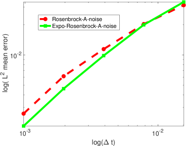
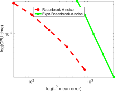
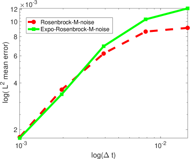
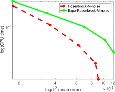
Figure 1: Convergence in the root mean square $L^{2}$ norm at $T=1$ as a function of $\Delta t$ for additive noise (a) and multiplicative noise (c). We take $\beta=2$, and $\epsilon=10^{-1}$ in relation (137) and use 80 realizations. Graph (b) and graph (d) show the CPU time per sample versus the root mean square $L^{2}$ errors for additive noise and multiplicative noise respectively.

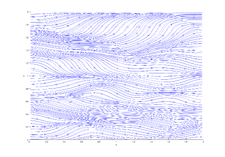
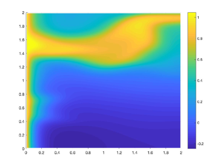
Figure 2: (a) The streamline of velocity (a) and a sample of the numerical solution with the stochastic Rosenbrock scheme for additive noise.

We take $L_{1}=2$ and $L_{2}=2$ and our reference solutions samples are numerical solutions with time step $\Delta t=1/2048$. The errors are computed at the final time $T=1$. The initial solution is $X_{0}=0$, so we can therefore expect high orders convergence, which depend only on the noise term. For both additive and multiplicative noise, we use $\beta=2$ and $\epsilon=10^{-1}$. The streamline of velocity is given at Figure 2(a) while a sample of the numerical solution with the stochastic Rosenbrock scheme for additive noise is given at Figure 2(b). In Figure 1(a) and Figure 1(c), the graphs of strong errors versus the time steps are plotting for stochastic Rosenbrock scheme and exponential Rosenbrock for additive noise and multiplicative noise respectively. The orders of convergence are $0.59$ (exponential Rosenbrock scheme) and $0.55$ (Rosenbrock scheme) for multiplicative noise, $1.03$ (exponential Rosenbrock scheme) and $0.92$ (Rosenbrock scheme) for additive noise, which are close to $0.5$ and $1$ in our theoretical results in Theorem 2.2 and Theorem 2.3 respectively. The implementation of the stochastic Rosenbrock-type scheme is straightforward and only need the resolution of a linear system of equations at each time step. For efficiency, all linear systems are solved using the Matlab function bicgstab coupled with ILU(0) preconditioners with no fill-in. The ILU(0) are done on the deterministic part of the the matrice $A_{h}$, that is $(I+\Delta tA_{h})$, at each time step. Figure 1(b) and Figure 1(d) show the mean of CPU time per sample versus the root mean square $L^{2}$ errors corresponding for Figure 1(a)(additive noise) and Figure 1(c)(multiplicative noise) respectively. As we can observe, the novel stochastic Rosenbrock scheme is more efficient than the stochastic exponential Rosenbrock scheme, thanks to the preconditioners.

References

- [1] K. J. Engel, R. Nagel, One-Parameter Semigroup for Linear Evolution Equations, Springer-Verlag, New York, Inc, 2000.
- [2] F. Fujita, T. Suzuki, Evolution problems (Part 1). Handbook of Numerical Analysis (P. G. Ciarlet and J.L. Lions eds), vol. 2. Amsterdam, The Netherlands: North-Holland, 1991, pp. 789–928.
- [3] S. Geiger, G. J. Lord, A. Tambue, Exponential time integrators for stochastic partial differential equations in 3D reservoir simulation, Computational Geosciences, 16(2)(2012) 323 – 334. https://doi:I 10.1007/s10596-011-9273-z
- [4] E. Hairer, Ch. Lubich, M. Roche, Error of Rosenbrock methods for stiff problems studied via differential algebraic equations, BIT 29 (1989) 77–90. https://doi.org/10.1007/BF01932707
- [5] E. Hairer, G. Wanner, Solving ordinary differential equations II. Siff and differential-algebraic problems, Springer-Verlag, Berlin, Heidelberg, 1991.
- [6] D. Henry, Geometric Theory of semilinear parabolic Equations, Lecture notes in Mathematics, vol. 840. Berlin : Springer, 1981.
- [7] M. Hochbruck, A. Ostermann, J. Schweitzer, Exponential Rosenbrock-type methods, SIAM J. Numer. Anal. 47(1)(2009) 786–803. https://doi.org/10.1137/080717717
- [8] A. Jentzen, P.E. Kloeden, Overcoming the order barrier in the numerical approximation of stochastic partial differential equations with additive space-time noise, Proc. R. Soc. Lond. Ser. A Math. Phys. Eng. Sci. 465(2102)(2009) 649–667. https://doi.org/10.1098/rspa.2008.0325
- [9] A. Jentzen, P. E. Kloeden, G. Winkel, Efficient simulation of nonlinear parabolic SPDEs with additive noise, Ann. Appl. Probab. 21(3)(2011) 908–950. https://www.jstor.org/stable/23033359
- [10] A. Jentzen, M. Röckner, Regularity analysis for stochastic partial differential equations with nonlinear multiplicative trace class noise, J. Diff. Equat. 252(1)(2012) 114–136. https://doi.org/10.1016/j.jde.2011.08.050
- [11] M. Kovács, S. Larsson, F. and Lindgren, Strong convergence of the finite element method with truncated noise for semilinear parabolic stochastic equations with additive noise, Numer. Algor. 53(2010) 309–220. https://doi.org/10.1007/s11075-009-9281-4
- [12] R. Kruse, Optimal error estimates of Galerkin finite element methods for stochastic partial differential equations with multiplicative noise, IMA J. Numer. Anal. 34(1)(2014) 217–251. https://doi.org/10.1093/imanum/drs055
- [13] R. Kruse, S. Larsson, Optimal regularity for semilinear stochastic partial differential equations with multiplicative noise, Electron. J. Probab. 17(65)(2012) 1–19. https://doi:10.1214/EJP.v17-2240
- [14] J. Lang, Adaptive Multilevel Solution of Nonlinear Parabolic PDE Systems. Theory, Algorithm, and Applications, Lecture Notes in Computational Sciences and Engineering, Vol. 16, Springer Verlag, 2000.
- [15] S. Larsson, Nonsmooth data error estimates with applications to the study of the long-time behavior of finite element solutions of semilinear parabolic problems, Preprint 1992-36, Department of Mathematics, Chalmers University of Technology, 1992. Available at: http://citeseerx.ist.psu.edu/viewdoc/summary?doi=10.1.1.28.1250
- [16] G. J. Lord, A. Tambue, Stochastic exponential integrators for the finite element discretization of SPDEs for multiplicative & additive noise, IMA J. Numer. Anal. 2(2013) 515–543. https://doi.org/10.1093/imanum/drr059
- [17] G. J. Lord, A. Tambue, A modified semi-implicit Euler-Maruyama scheme for finite element discretization of SPDEs with additive noise, Appl. Math. Comput. 332(2018) 105–122. https://doi.org/10.1016/j.amc.2018.03.014
- [18] Ch. Lubich, O. Nevanlina, On the resolvent conditions and stability estimates, BIT 31(1991) 293–313. https://doi.org/10.1007/BF01931289
- [19] J. D. Mukam, A. Tambue, Strong convergence analysis of the stochastic exponential Rosenbrock scheme for the finite element discretization of semilinear SPDEs driven by multiplicative and additive noise, J. Sci. Comput. 74(2018) 937–978. https://doi.org/10.1007/s10915-017-0475-y
- [20] J. D. Mukam, A. Tambue, A note on exponential Rosenbrock-Euler method for the finite element discretization of a semilinear parabolic partial differential equation, Comput. Math. Appl. 76(7)(2018) 1719–1738. https://doi.org/10.1016/j.camwa.2018.07.025
- [21] A. Ostermann, M. Roche, Rosenbrock methods for partial differential equations and fractional orders of convergence, SIAM J. Numer. 30(4)(1993) 1084–1098. https://doi.org/10.1137/0730056
- [22] A. Ostermann, M. Thalhammer, Non-smooth data error estimates for linearly implicit Runge-Kutta methods, IMA J. Numer. Anal. 20(2000) 167–184. https://doi.org/10.1093/imanum/20.2.167
- [23] K. Paps, G. Wanner, A study of Rosenbrock-type methods of higher order, Numer. Math. 38(1981) 279–298. https://doi.org/10.1007/BF01397096
- [24] A. Pazy, Semigroups of Linear Operators and Applications to Partial Differential Equations, Applied Mathematical Sciences; Springer-Verlag, New York, v 44, 1983.
- [25] D. Prato, G. J. Zabczyk, Stochastic equations in infinite dimensions, vol 152. Cambridge, United Kingdom: Cambrige University Press, 2014.
- [26] J. Printems On the discretization in time of parabolic stochastic partial differential equations, Math. modelling and numer. Anal. 35(6)(2001) 1055–1078. https://doi.org/10.1051/m2an:2001148
- [27] C. Prévôt, M. Röckner, A Concise Course on Stochastic Partial Differential Equations, Lecture Notes in Mathematics, vol. 1905, Springer, Berlin, 2007.
- [28] T. Shardlow, Numerical simulation of stochastic PDEs for excitable media, J. Comput. Appl. Math. 175(2)(2005) 429–446. https://doi.org/10.1016/j.cam.2004.06.020
- [29] A. Tambue, Efficient Numerical Schemes for Porous Media Flow. PhD Thesis, Department of Mathematics, Heriot–Watt University, 2010.
- [30] A. Tambue, An exponential integrator for finite volume discretization of a reaction-advection-diffusion equation, Comput. Math. Appl. 71(9)(2016) 1875–1897. https://doi.org/10.1016/j.camwa.2016.03.001
- [31] A. Tambue, G. J. Lord, S. Geiger, An exponential integrator for advection-dominated reactive transport in heterogeneous porous media, Journal of Computational Physics, 229(10)(2010) 3957–3969. https://doi.org/10.1016/j.jcp.2010.01.037
- [32] A. Tambue, I. Berre, J. M. Nordbotten, Efficient simulation of geothermal processes in heterogeneous porous media based on the exponential Rosenbrock–Euler and Rosenbrock-type methods, Advances in Water Resources, 53(2013) 250–262. https://doi.org/10.1016/j.advwatres.2012.12.004
- [33] A. Tambue, J. D. Mukam, Strong convergence of the linear implicit Euler method for the finite element discretization of semilinear SPDEs driven by multiplicative and additive noise, Appl. Math. Comput. 346(2019) 23–40. https://doi.org/10.1016/j.amc.2018.09.073
- [34] X. Wang, Q. Ruisheng, A note on an accelerated exponential Euler method for parabolic SPDEs with additive noise, Appl. Math. Lett. 46(2015) 31–37. https://doi.org/10.1016/j.aml.2015.02.001
- [35] X. Wang, Strong convergence rates of the linear implicit Euler method for the finite element discretization of SPDEs with additive noise, IMA J. Numer. Anal. 37(2)(2017) 965–984. https://doi.org/10.1093/imanum/drw016
- [36] Y. Yan, Galerkin finite element methods for stochastic parabolic partial differential equations, SIAM J. Num. Anal. 43(4)(2005) 1363–1384. https://doi.org/10.1137/040605278
- [37] Y. Yan, Semidiscrete Galerkin approximation for a linear stochastic parabolic partial differential equation driven by an additive noise, BIT Numer. Math. 44(4)(2004) 829–847. https://doi.org/10.1007/s10543-004-3755-5