MPP–2018–28
EMPG–18–05

Symplectic realisation of electric charge
in fields of monopole distributions

Vladislav G. Kupriyanov¹  and  Richard J. Szabo²

¹ Max-Planck-Institut für Physik, Werner-Heisenberg-Institut
Föhringer Ring 6, 80805 München, Germany
and CMCC-Universidade de Federal do ABC, Santo André, SP, Brazil
and Tomsk State University, Tomsk, Russia
Email:  vladislav.kupriyanov@gmail.com
² Department of Mathematics, Heriot-Watt University
Colin Maclaurin Building, Riccarton, Edinburgh EH14 4AS, U.K.
and Maxwell Institute for Mathematical Sciences, Edinburgh, U.K.
and The Higgs Centre for Theoretical Physics, Edinburgh, U.K.
Email:  R.J.Szabo@hw.ac.uk

We construct a symplectic realisation of the twisted Poisson structure on the phase space of an electric charge in the background of an arbitrary smooth magnetic monopole density in three dimensions. We use the extended phase space variables to study the classical and quantum dynamics of charged particles in arbitrary magnetic fields by constructing a suitable Hamiltonian that reproduces the Lorentz force law for the physical degrees of freedom. In the source-free case the auxiliary variables can be eliminated via Hamiltonian reduction, while for non-zero monopole densities they are necessary for a consistent formulation and are related to the extra degrees of freedom usually required in the Hamiltonian description of dissipative systems. We obtain new perspectives on the dynamics of dyons and motion in the field of a Dirac monopole, which can be formulated without Dirac strings. We compare our associative phase space formalism with the approach based on nonassociative quantum mechanics, reproducing extended versions of the characteristic translation group three-cocycles and minimal momentum space volumes, and prove that the two approaches are formally equivalent. We also comment on the implications of our symplectic realisation in the dual framework of non-geometric string theory and double field theory.

1 Introduction and summary

Despite their elusiveness to experimental observation, magnetic monopoles have been of wide-spread theoretical interest in various areas of physics for many years due to their novel conceptual and mathematical implications. In particular, the quantum mechanics of an electric charge coupled to a magnetic monopole density exhibits a variety of interesting geometric and algebraic features. For the standard example of motion in the field of a Dirac monopole, the charged particle wavefunction can be regarded as a section of a non-trivial line bundle associated to the Hopf fibration [51] which provides a topological explanation for Dirac charge quantisation [21, 22] and formulates the quantum dynamics of the particle without using the unphysical Dirac string singularities that usually arise due to the absence of a globally defined magnetic vector potential for the monopole field.

In this paper we are predominantly interested in smooth distributions of magnetic charge, for which vector potentials do not exist even locally and the classical dynamics of the canonical phase space coordinates of the particle are described by a necessarily nonassociative twisted Poisson algebra. These systems have been of interest recently as magnetic analogues of certain flux models in non-geometric string theory and double field theory, see e.g. [39, 4, 11, 43, 40] and references therein. In these instances the corresponding quantum theory cannot be formulated in the usual framework of canonical quantisation by operators acting on a separable Hilbert space. Two formulations have thus far been proposed to handle nonassociative quantum mechanics in this setting, each with its own limitations. Deformation quantisation by explicit construction of nonassociative phase space star products was originally developed by [41], and subsequently treated in [4, 42, 36]; however, beyond the case of constant magnetic charge density, this procedure does not yield a quantisation of the classical dynamical system because the Planck constant $\hbar$ appears as a formal expansion parameter, and the result is a deformation over an algebra of formal power series rather than with a complex parameter. On the other hand, the approach of [12, 13] is based on developing algebraic properties of quantum moments from the assumption that the underlying twisted Poisson algebra is a Malcev algebra; however, even in the simplest case of constant monopole density, the alternative property used there cannot be realised in general and this formalism is restricted to observables which are linear in the kinematical momenta.

The purpose of the present paper is to develop a new approach to the classical and quantum dynamics of electric charges in monopole distributions by generalising the technique of ‘symplectic realisation’ from Poisson geometry [49, 32, 50, 19]. Symplectic realisation is a useful mathematical tool for quantisation, because it embeds arbitrary Poisson manifolds into the framework of geometric quantisation or other standard quantisation methods based on symplectic structures. In the following we construct a symplectic realisation of the twisted Poisson structure corresponding to the algebra of covariant momenta of a charged particle in the background of an arbitrary monopole field. This construction doubles the original phase space coordinates by introducing a set of auxiliary degrees of freedom. The resulting associative extended algebra of Poisson brackets is then used to construct a Hamiltonian description of a charged particle interacting with a distribution of magnetic monopoles, by an appropriate choice of Hamiltonian on the extended phase space that leads to the Lorentz force equation for the physical coordinates. In the case of a magnetic field with no monopole sources, one can eliminate the auxiliary variables by Hamiltonian reduction and thus recover the standard Hamiltonian formulation of a charged particle in a divergenceless magnetic field. However, in the presence of magnetic monopoles, the auxiliary degrees of freedom are necessary for a consistent Hamiltonian description. In the particular example of a spherically symmetric magnetic field sourced by a constant monopole density, we show that Hamiltonian reduction results either in free particle motion or in the absence of propagating degrees of freedom altogether. We demonstrate that the necessary presence of auxiliary degrees of freedom in this case is related to the fact that the motion of a charged particle can be effectively described as motion in the field of a single Dirac monopole with some frictional forces [4], and normally the consistent Hamiltonian description of a system with friction requires the introdution of additional degrees of freedom representing a reservoir.

With this set up, quantisation then proceeds along the usual lines using canonical methods by constructing a suitable Hilbert space on which the quantum Hamiltonian operator acts, and studying the Schrödinger equation. Our formalism mimicks the standard quantisation schemes which assume that the phase space is topologically trivial and that the magnetic field has a globally defined vector potential. In standard approaches this is not the case even for the Dirac monopole field. Our formalism also provides a new perspective on the quantisation of a charged particle in the field of a Dirac monopole, in that our extended vector potentials are constructed without the usual Dirac string singularities [21, 22]. In this respect our approach of employing extended coordinates is reminescent of old approaches to the description of electrodynamics with electric and magnetic sources in terms of two vector potentials [15], which also avoids the pathologies associated to the unphysical Dirac string; however, this latter formulation necessitates Dirac charge quantisation for consistency, whereas our approach does not. Our constructions analogously have a natural extension to settings which respect electromagnetic duality, and when applied to the dynamics of dyons, our formalism circumvents the usual problems with defining electromagnetically dual vector potentials. Gauge theory versions of (ordinary associative) phase space doubling were introduced by [23, 24] for dealing with Schwinger terms viewed as cocycles, and more generally by [5, 6] for dealing with second class constraints; see [25] for an application of this formalism to the superparticle and to the Proca Lagrangian.

We will demonstrate that the symplectic realisation which we develop is equivalent to the framework of nonassociative phase space quantum mechanics in terms of star products of states and composition products of observables [42], see [48] for a review in the setting of the present paper. On the other hand, our framework avoids the problems with constructing star products for spatially varying monopole densities. Our formalism should reproduce the quantum fluctuations which compute the quantum evolution of basic dynamical variables from [12, 13], which demonstrate that the nonassociative dynamics generically exhibit modifications of the classical Lorentz force law (but we do not check this in detail). In our formalism based on an extended phase space we are able to reproduce the novel predictions of nonassociative quantum mechanics within an associative approach, such as an extended realisation of the three-cocycle of the translation group which obstructs a projective representation on the charged particle wavefunctions, and also of the minimal uncertainty volumes due to non-vanishing associators. The latter are particularly interesting in the string theory dual models where they imply a coarse-graining of spacetime [9, 38, 42]. Indeed, our framework is analogous to the locally ‘non-geometric’ backgrounds in string theory, wherein there are no local expressions for the geometry and the background fields require the extended space of double field theory for their proper definition. In particular, as discussed by e.g. [40], the uniform magnetic charge density is the magnetic analogue of the locally non-geometric $R$-flux background of string theory in three dimensions. Our approach bears certain qualitative similarities to double field theory, such as an underlying $O(3,3)\times O(3,3)$ symmetry of the dynamics on the extended phase space, but also certain important differences that we discuss in the following.

The outline of the remainder of this paper is as follows. In Section 2 we introduce our symplectic realisation of the twisted Poisson algebra governing the kinematics of an electric charge in a generic magnetic background; our approach generalises the standard symplectic realisations of Poisson structures whose technical details we briefly describe in Appendix A. In Section 3 we demonstrate how to construct a suitable Hamiltonian on the extended phase space which reproduces the classical Lorentz force law for the physical degrees of freedom, while in Section 4 we analyse in detail the problem of classical Hamiltonian reduction, or polarisation, of the extended dynamics. In Section 5 we extend our formalism in a way which respects electromagnetic duality and describe the ensuing dynamics of dyons within our symplectic realisation. In Section 6 we address the problem of explicitly integrating the equations of motion for a charged particle in a magnetic monopole background; for spherically symmetric magnetic fields sourced by constant monopole densities we relate the classical dynamics on extended phase space to that of dissipative systems, which is reviewed briefly in Appendix B, and we show that the equations of motion are integrable in the case of axial magnetic fields, obtaining the explicit solution which is analogous to motion in the source-free case. In Section 7 we consider the quantum dynamics in the symplectic realisation, demonstrating how the extended formalism reproduces the expected results in source-free cases, and exploiting the connections to quantum dissipation discussed in Appendix B. In Section 8 we demonstrate how our extended associative formulation captures features of nonassocative quantum mechanics, and in Section 9 we show that the symplectic realisation is formally equivalent to the phase space formulation of nonassociative quantum mechanics in terms of star products and composition products. A final Appendix C compares the extended phase space of the symplectic realisation to the phase space of locally non-geometric closed strings and double field theory, and also presents potential applications of our formalism in non-geometric M-theory.

2 Symplectic realisation of the magnetic monopole algebra

The phase space $\mathcal{P}$ of a nonrelativistic point particle with electric charge $e$ and mass $m$ in a magnetic field $\vec{B}(\vec{x}\,)$ in three dimensions is parameterised by position coordinates $\vec{x}\in{\mathbb{R}}^{3}$ and the kinematical momentum variables $\vec{\bar{\pi}}=m\,\dot{\vec{x}}$, where an overdot denotes a time derivative. The coordinate algebra is defined by the brackets

$$\{x^{i},x^{j}\}=0\ ,\quad\{x^{i},\bar{\pi}_{j}\}=\delta^{i}{}_{j}\qquad\mbox{and}\qquad\{\bar{\pi}_{i},\bar{\pi}_{j}\}=e\,\varepsilon_{ijk}\,B^{k}(\vec{x}\,)\ ,$$ (2.1)

where throughout we set the speed of light to $c=1$. These brackets are equivalent to an almost symplectic structure on $\mathcal{P}$, i.e. a non-degenerate two-form on phase space given by

$$\omega=\mbox{$\frac{e}{2}$}\,\varepsilon_{ijk}\,B^{k}(\vec{x}\,)\ {\rm d}x^{i}\wedge{\rm d}x^{j}+{\rm d}\bar{\pi}_{i}\wedge{\rm d}x^{i}\ ,$$ (2.2)

which is not generally closed: The Jacobiator amongst the momenta $\bar{\pi}_{i}$ is given by

$$\{\bar{\pi}_{i},\bar{\pi}_{j},\bar{\pi}_{k}\}:=\mbox{$\frac{1}{3}$}\,\{\bar{\pi}_{i},\{\bar{\pi}_{j},\bar{\pi}_{k}\}\}+\mbox{cyclic}=e\,\varepsilon_{ijk}\,\vec{\nabla}\cdot\vec{B}\ .$$ (2.3)

Thus the brackets (2.1) generically define a twisted Poisson structure on the six-dimensional phase space, with twisting three-form $\tau={\rm d}\omega=\frac{e}{3!}\,\varepsilon_{ijk}\,(\vec{\nabla}\cdot\vec{B}\,)\,{\rm d}x^{i}\wedge{\rm d}x^{j}\wedge{\rm d}x^{k}$ on the configuration space.

In classical Maxwell theory one has $\vec{\nabla}\cdot\vec{B}=0$, so that the Jacobiator (2.3) vanishes and the algebra (2.1) is associative. In this case the magnetic field can be written as $\vec{B}=\vec{\nabla}\times\vec{a}$ for a globally defined smooth vector potential $\vec{a}(\vec{x}\,)$ on ${\mathbb{R}}^{3}$, and the Poisson algebra can be represented by transforming the symplectic two-form (2.2) to the standard symplectic structure $\omega={\rm d}p_{i}\wedge{\rm d}x^{i}$ for the canonically conjugate position and momentum coordinates $\vec{x}$ and $\vec{p}=\vec{\bar{\pi}}+e\,\vec{a}$.

For the spherically symmetric field

$$\vec{B}_{\rm D}(\vec{x}\,)=g\,\frac{\vec{x}}{|\vec{x}\,|^{3}}$$ (2.4)

of a Dirac monopole at the origin with magnetic charge $g$, the algebra is associative at every point away from the location of the monopole. In this case one can excise the origin, where $\vec{B}_{\rm D}$ is singular, and locally define a corresponding vector potential [54]

$$\vec{a}_{\rm D}(\vec{x}\,)=\frac{g}{|\vec{x}\,|}\,\frac{\vec{x}\times\vec{n}}{|\vec{x}\,|-\vec{x}\cdot\vec{n}}$$ (2.5)

at every position $\vec{x}$ of the configuration space ${\mathbb{R}}^{3}\setminus\{\vec{0}\,\}$, which has a smaller domain of regularity obtained by removing a Dirac string singularity [21, 22] along the line in the direction of the fixed unit vector $\vec{n}$ from the origin to infinity in ${\mathbb{R}}^{3}$. The exclusion of the origin from the configuration space implies that the charged particle and the monopole cannot simultaneously occupy the same point in space.

In the present paper we are primarily interested in smooth distributions of magnetic poles, where $\vec{\nabla}\cdot\vec{B}\neq 0$ on a connected dense open subset of ${\mathbb{R}}^{3}$. In this case there is no associated local vector potential and the algebra (2.1) is nonassociative on the entire configuration space ${\mathbb{R}}^{3}$. We call it the magnetic monopole algebra.

In this section we will construct a symplectic embedding of the magnetic monopole algebra. For this, let us introduce an extended $12$-dimensional phase space $\mathscr{P}$ with position coordinates $x^{I}=(x^{i},\tilde{x}^{i})$ and momentum coordinates $p_{I}=(p_{i},\tilde{p}_{i})$, where $i=1,2,3$ and $I=1,\dots,6$, which have the canonical Poisson brackets $\{x^{I},x^{J}\}=\{p_{I},p_{J}\}=0$ and $\{x^{I},p_{J}\}=\delta^{I}{}_{J}$. We define the “covariant” momenta associated to the magnetic field $\vec{B}(\vec{x}\,)$ by

$$\pi_{I}=\left(\pi_{i},\tilde{\pi}_{i}\right)=p_{I}-e\,A_{I}(x^{I})\ ,$$ (2.6)

with the corresponding magnetic Poisson brackets

$$\{\pi_{I},\pi_{J}\}=e\,F_{IJ}(x^{I})\qquad\mbox{with}\quad F_{IJ}=\partial_{I}A_{J}-\partial_{J}A_{I}\ ,$$ (2.7)

where $\partial_{I}=\frac{\partial}{\partial x^{I}}$. We choose the magnetic vector potential $A_{I}=(A_{i},{\tilde{A}}_{i})$ as

$$\vec{A}(x^{I})=-\mbox{$\frac{1}{2}$}\,\vec{\tilde{x}}\times\vec{B}(\vec{x}\,)\qquad\mbox{and}\qquad\vec{\tilde{A}}(x^{I})=\vec{0}\ .$$ (2.8)

It has the property

$$\vec{\tilde{\nabla}}\times\vec{A}=\vec{B}\ ,$$ (2.9)

where $\vec{\tilde{\nabla}}$ are the directional derivatives along the extended configuration space directions $\vec{\tilde{x}}$, which we denote by $\tilde{\partial}{}_{i}=\frac{\partial}{\partial\tilde{x}{}^{i}}$. The non-vanishing Poisson brackets read

$$\{x^{i},\pi_{j}\} = \{\tilde{x}^{i},\tilde{\pi}_{j}\}\ \ =\ \ \delta^{i}{}_{j}\ ,$$

$$\{\pi_{i},\pi_{j}\} = \mbox{$\frac{e}{2}$}\,\big{(}\varepsilon_{ijk}\,\partial_{l}B^{k}(\vec{x}\,)-\varepsilon_{ijl}\,\partial_{k}B^{k}(\vec{x}\,)\big{)}\,\tilde{x}^{l}\ ,$$

$$\{\pi_{i},\tilde{\pi}_{j}\} = \{\tilde{\pi}_{i},\pi_{j}\}\ \ =\ \ \mbox{$\frac{e}{2}$}\,\varepsilon_{ijk}\,B^{k}(\vec{x}\,)\ .$$ (2.10)

The algebra (2.10) defines a symplectic structure, and (2.6) expresses $\pi_{I}$ in terms of the Darboux coordinates $x^{I}$ and $p_{I}$.

To relate (2.10) with the magnetic monopole algebra (2.1) we introduce

$$\vec{\bar{\pi}}=\vec{\pi}+\vec{\tilde{\pi}}\ .$$ (2.11)

The vanishing brackets are

$$\{x^{i},x^{j}\}=\{x^{i},\tilde{x}^{j}\}=\{\tilde{x}^{i},\tilde{x}^{j}\}=\{x^{i},\tilde{\pi}_{j}\}=\{\tilde{\pi}_{i},\tilde{\pi}_{j}\}=0\ ,$$ (2.12)

while the non-vanishing brackets are given by

$$\{x^{i},\bar{\pi}_{j}\} = \{\tilde{x}^{i},\bar{\pi}_{j}\}\ \ =\ \ \{\tilde{x}^{i},\tilde{\pi}_{j}\}\ \ =\ \ \delta^{i}{}_{j}\ ,$$

$$\{\bar{\pi}_{i},\bar{\pi}_{j}\} = e\,\varepsilon_{ijk}\,B^{k}(\vec{x}\,)+\mbox{$\frac{e}{2}$}\,\big{(}\varepsilon_{ijk}\,\partial_{l}B^{k}(\vec{x}\,)-\varepsilon_{ijl}\,\partial_{k}B^{k}(\vec{x}\,)\big{)}\,\tilde{x}^{l}\ ,$$

$$\{\bar{\pi}_{i},\tilde{\pi}_{j}\} = \{\tilde{\pi}_{i},\bar{\pi}_{j}\}\ \ =\ \ \mbox{$\frac{e}{2}$}\,\varepsilon_{ijk}\,B^{k}(\vec{x}\,)\ .$$ (2.13)

The symplectic two-form on the extended phase space $\mathscr{P}$ corresponding to the Poisson brackets (2.13) is given by

$$\Omega = \mbox{$\frac{e}{2}$}\,\big{[}\,\varepsilon_{ijk}\,B^{k}(\vec{x}\,)+\mbox{$\frac{1}{2}$}\,\big{(}\varepsilon_{ijk}\,\partial_{l}B^{k}(\vec{x}\,)-\varepsilon_{ijl}\,\partial_{k}B^{k}(\vec{x}\,)\big{)}\,\tilde{x}^{l}\,\big{]}\ {\rm d}x^{i}\wedge{\rm d}x^{j}+\mbox{$\frac{e}{2}$}\,\varepsilon_{ijk}\,B^{k}(\vec{x}\,)\ {\rm d}x^{i}\wedge{\rm d}\tilde{x}^{j}$$ (2.14)

$$+\,{\rm d}\bar{\pi}_{i}\wedge{\rm d}x^{i}+{\rm d}\bar{\pi}_{i}\wedge{\rm d}\tilde{x}^{i}+{\rm d}\tilde{\pi}_{i}\wedge{\rm d}\tilde{x}^{i}\ .$$

There is a natural projection ${\sf p}:\mathscr{P}\to\mathcal{P}$ with ${\sf p}(\vec{x},\vec{\tilde{x}},\vec{\bar{\pi}},\vec{\tilde{\pi}}\,)=(\vec{x},\vec{\bar{\pi}}\,)$, under which our original phase space $\mathcal{P}$ can be embedded into $\mathscr{P}$ as the zero section ${\sf s}_{0}:\mathcal{P}\to\mathscr{P}$ with ${\sf s}_{0}(\vec{x},\vec{\bar{\pi}}\,)=(\vec{x},\vec{0},\vec{\bar{\pi}},\vec{0}\,)$. Then the pullback of (2.14) to the constraint surface $\mathscr{C}_{0}\subset\mathscr{P}$ defined by $\vec{\tilde{x}}=\vec{\tilde{\pi}}=\vec{0}$ coincides exactly with the almost symplectic structure (2.2), i.e. ${\sf s}_{0}^{*}\,\Omega=\Omega|_{\mathscr{C}_{0}}=\omega$. This therefore determines a symplectic realisation of the twisted Poisson structure on $\mathcal{P}$ (see Appendix A), and it is in this sense that we refer to (2.13) as a symplectic realisation of the magnetic monopole algebra (2.1).

An important example of a symplectic realisation of the magnetic monopole algebra corresponds to a constant and uniform magnetic charge distribution with density $\vec{\nabla}\cdot\vec{B}=\rho$. In this paper we will study in detail two particular examples of corresponding magnetic fields. A magnetic field with spherical symmetry is given by

$$\vec{B}_{\rm spher}(\vec{x}\,)=\mbox{$\frac{\rho}{3}$}\,\vec{x}\ ,$$ (2.15)

with the symplectic algebra

$$\{x^{i},\bar{\pi}_{j}\} = \{\tilde{x}^{i},\bar{\pi}_{j}\}\ \ =\ \ \{\tilde{x}^{i},\tilde{\pi}_{j}\}\ \ =\ \ \delta^{i}{}_{j}\ ,$$

$$\{\bar{\pi}_{i},\bar{\pi}_{j}\} = \mbox{$\frac{e\,\rho}{3}$}\,\,\varepsilon_{ijk}\,\big{(}x^{k}-\tilde{x}^{k}\big{)}\ ,$$

$$\{\bar{\pi}_{i},\tilde{\pi}_{j}\} = \{\tilde{\pi}_{i},\bar{\pi}_{j}\}\ \ =\ \ \mbox{$\frac{e\,\rho}{6}$}\,\varepsilon_{ijk}\,x^{k}\ .$$ (2.16)

As discussed in [40], the uniform magnetic charge density $\rho$ can be interpreted as a smearing of infinitely many densely distributed Dirac monopoles of charge $g=\rho$ and magnetic fields $\vec{B}_{\rm D}(\vec{x}-\vec{y}\,)$, and in this setting there is a formal non-local magnetic vector potential for (2.15). The gauge field on the extended configuration space from (2.8) in this case,

$$\vec{A}_{\rm spher}(x^{I})=-\mbox{$\frac{\rho}{6}$}\,\vec{\tilde{x}}\times\vec{x}\qquad\mbox{and}\qquad\vec{\tilde{A}}_{\rm spher}(x^{I})=\vec{0}\ ,$$ (2.17)

is a vector potential for (2.15) in the sense of (2.9). This gives a precise meaning to the absence of a local definition of the vector potential and to the formal non-local smeared expression derived in [40]: A definition of fields of smooth magnetic charge distributions akin to classical Maxwell theory necessitates the symplectic realisation of the magnetic monopole algebra. It is this feature that we shall exploit in the following which makes the classical and quantum dynamics tractable.

At the opposite extreme, we can break spherical symmetry by choosing an axial magnetic field which is oriented in the direction of a fixed vector in ${\mathbb{R}}^{3}$; this is the analogue of a static uniform magnetic field in the source-free case. We can choose coordinates in which this direction is along the $z$-axis and take the linear magnetic field

$$\vec{B}_{\rm axial}(\vec{x}\,)=(0,0,\rho\,z)\ ,$$ (2.18)

where $\vec{x}=(x,y,z)$. This leads to the symplectic algebra

$$\{x^{i},\bar{\pi}_{j}\} = \{\tilde{x}^{i},\bar{\pi}_{j}\}\ \ =\ \ \{\tilde{x}^{i},\tilde{\pi}_{j}\}\ \ =\ \ \delta^{i}{}_{j}\ ,$$

$$\{\bar{\pi}_{x},\bar{\pi}_{y}\} = e\,\rho\,z\ ,\qquad\{\bar{\pi}_{x},\bar{\pi}_{z}\}\ \ =\ \ \mbox{$\frac{e\,\rho}{2}$}\,\tilde{y}\qquad\mbox{and}\qquad\{\bar{\pi}_{y},\bar{\pi}_{z}\}\ \ =\ \ -\mbox{$\frac{e\,\rho}{2}$}\,\tilde{x}\ ,$$

$$\{\bar{\pi}_{x},\tilde{\pi}_{y}\} = \{\tilde{\pi}_{x},\bar{\pi}_{y}\}\ \ =\ \ \mbox{$\frac{e\,\rho}{2}$}\,z\ .$$ (2.19)

The corresponding vector potential on the extended configuration space is given by

$$\vec{A}_{\rm axial}(x^{I})=\mbox{$\frac{\rho}{2}$}\,(-\tilde{y}\,z,\tilde{x}\,z,0)\qquad\mbox{and}\qquad\vec{\tilde{A}}_{\rm axial}(x^{I})=\vec{0}\ .$$ (2.20)

Both magnetic fields (2.15) and (2.18) correspond to a uniform magnetic charge distribution of density $\rho$, as $\vec{\nabla}\cdot\vec{B}_{\rm spher}=\vec{\nabla}\cdot\vec{B}_{\rm axial}=\rho$, and their difference is a divergenceless magnetic field

$$\vec{B}_{\rm axial}(\vec{x}\,)-\vec{B}_{\rm spher}(\vec{x}\,)=\vec{\nabla}\times\mbox{$\frac{2}{3}$}\,\vec{A}_{\rm axial}(\vec{x},\vec{x}\,)\ ,$$ (2.21)

which therefore does not contribute to the distribution of magnetic charge. However, it does contribute to the twisted Poisson structure defining the magnetic monopole algebra (2.1). Specifying only the equation $\vec{\nabla}\cdot\vec{B}=\rho$ does not uniquely define the corresponding magnetic field $\vec{B}$ so that, in contrast to the magnetic field (2.4) of a Dirac monopole, here we cannot apply considerations of spherical symmetry and the fact that the field should be directed from the origin to fix the form of $\vec{B}$. From a geometric perspective, the Poisson algebra (2.7) is invariant under the usual one-form gauge transformations $A_{I}\mapsto A_{I}+\partial_{I}\chi$ on ${\mathbb{R}}^{6}$, as in this case $A_{I}(x^{I})$ defines a gauge field associated to a trivial $U(1)$-bundle over the extended configuration space. However, it is not invariant under the higher two-form gauge transformations $\vec{B}\mapsto\vec{B}+\vec{\nabla}\times\vec{a}$ of the magnetic field on ${\mathbb{R}}^{3}$, which preserve the curvature $\vec{\nabla}\cdot\vec{B}=\rho$. The essential geometric feature is that the field of a constant and uniform magnetic charge distribution defines a “higher” gauge field associated to a $U(1)$-gerbe on ${\mathbb{R}}^{3}$, contrary to the field of a Dirac monopole which defines a gauge field of a non-trivial $U(1)$-bundle over ${\mathbb{R}}^{3}\setminus\{\vec{0}\,\}$ of degree $g$; see [14, 40, 48] for further discussion of this point. This absence of higher gauge symmetry has profound physical consequences, as we shall see later on.

3 Classical dynamics from symplectic realisation

The classical motion of a spinless point particle of electric charge $e$ and mass $m$ under the influence of both a background magnetic field $\vec{B}(\vec{x}\,)$ and a background electric field $\vec{E}(\vec{x}\,)$ in three dimensions is governed by the Lorentz force

$$\frac{{\rm d}\vec{\bar{\pi}}}{{\rm d}t}=\frac{e}{m}\,\vec{\bar{\pi}}\times\vec{B}+e\,\vec{E}\ .$$ (3.1)

In this paper we assume that the electromagnetic backreaction due to acceleration of the charged particle is negligible, and treat the magnetic and electric fields in (3.1) as fixed prescribed backgrounds. As before, in this equation we need not assume that the magnetic field $\vec{B}$ is divergenceless, i.e. we include fields created by magnetic poles. If $\vec{\nabla}\times\vec{E}=\vec{0}$, the electric field can be represented as a gradient field $\vec{E}=\vec{\nabla}\phi$ for a globally defined smooth scalar potential $\phi(\vec{x}\,)$ on ${\mathbb{R}}^{3}$. In this case, the Lorentz force law (3.1), together with the definition $\dot{\vec{x}}=\vec{\bar{\pi}}/m$, can be written as the Hamilton equations of motion $\dot{x}^{i}=\{x^{i},{\mathcal{H}}\}$, $\dot{\bar{\pi}}_{i}=\{\bar{\pi}_{i},{\mathcal{H}}\}$ with the magnetic monopole algebra (2.1) and the Hamiltonian taken to be the sum of the kinetic energy and the electrostatic potential energy: ${\mathcal{H}}(\vec{x},\vec{\bar{\pi}}\,)=\vec{\bar{\pi}}^{\,2}/2m+e\,\phi(\vec{x}\,)$. When $\vec{\nabla}\times\vec{E}\neq\vec{0}$, for instance when magnetic currents are present, this is no longer possible when $\vec{\nabla}\cdot\vec{B}\neq 0$. Here we shall allow for more general electric fields in our formalism, i.e. we also allow for motion in the field of general smooth distributions of electric poles. This is natural from the present perspective, but we shall argue for it more precisely later on through considerations of electromagnetic duality. The purpose of this section is to demonstrate that the Lorentz force (3.1) follows in these generic situations from our symplectic realisation of the magnetic monopole algebra by choosing an appropriate Hamiltonian function ${\mathcal{H}}$ on the extended phase space $\mathscr{P}$.

For later use, we shall momentarily leave the explicit form of the vector potential $A_{I}(x^{I})$ in (2.6) unspecified. Since the Poisson brackets (2.7) do not depend on momentum, while the Lorentz force is linear in the kinematical momenta, the corresponding Hamiltonian is quadratic in the momenta and of the general form

$${\mathcal{H}}(x^{I},\pi_{I})=\frac{1}{2}\,\big{(}\begin{matrix}\vec{\pi}&\vec{\tilde{\pi}}\ \,\end{matrix}\big{)}\cdot\bigg{(}\begin{matrix}a&b\\ b&c\end{matrix}\bigg{)}\bigg{(}\begin{matrix}\,\vec{\pi}\ \,\\ \,\vec{\tilde{\pi}}\ \,\end{matrix}\bigg{)}+V(x^{I})\ ,$$ (3.2)

where $a$, $b$ and $c$ are real coefficients, and $V(x^{I})$ is a smooth potential energy function on the extended configuration space. The corresponding Hamilton equations of motion $\dot{x}^{I}=\{x^{I},{\mathcal{H}}\}$, $\dot{\pi}_{I}=\{\pi_{I},{\mathcal{H}}\}$ read

$$\dot{x}^{i} = a\,\pi^{i}+b\,{\tilde{\pi}}^{i}\ ,$$

$$\dot{\tilde{x}}^{i} = b\,\pi^{i}+c\,{\tilde{\pi}}^{i}\ ,$$

$$\dot{\pi}_{i} = \{\pi_{i},\pi_{j}\}\,(a\,\pi^{j}+b\,\tilde{\pi}^{j})+\{\pi_{i},\tilde{\pi}_{j}\}\,(b\,\pi^{j}+c\,{\tilde{\pi}}^{j})-\partial_{i}V\ ,$$

$$\dot{\tilde{\pi}}_{i} = \{\tilde{\pi}_{i},\pi_{j}\}\,(a\,\pi^{j}+b\,{\tilde{\pi}}^{j})+\{\tilde{\pi}_{i},\tilde{\pi}_{j}\}\,(b\,\pi^{j}+c\,{\tilde{\pi}}^{j})-\tilde{\partial}_{i}V\ ,$$ (3.3)

from which one obtains the coupled system of second order differential equations for the extended configuration space coordinates $x^{i}$ and $\tilde{x}^{i}$ given by

$$\ddot{x}^{i} = \{a\,\pi^{i}+b\,{\tilde{\pi}}^{i},\pi_{j}\}\,\dot{x}^{j}+\{a\,\pi^{i}+b\,{\tilde{\pi}}^{i},\tilde{\pi}_{j}\}\,\dot{\tilde{x}}^{j}-a\,\partial^{i}V-b\,{\tilde{\partial}}^{i}V\ ,$$ (3.4)

$$\ddot{\tilde{x}}^{i} = \{b\,\pi^{i}+c\,{\tilde{\pi}}^{i},\pi_{j}\}\,\dot{x}^{j}+\{b\,\pi^{i}+c\,{\tilde{\pi}}^{i},\tilde{\pi}_{j}\}\,\dot{\tilde{x}}^{j}-b\,\partial^{i}V+c\,{\tilde{\partial}}^{i}V\ .$$ (3.5)

If $a=0$, $b=2/m$, $\left\{\tilde{\pi}_{i},\tilde{\pi}_{j}\right\}=0$ and $\left\{\tilde{\pi}_{i},\pi_{j}\right\}=(e/2)\,\varepsilon_{ijk}\,B^{k}(\vec{x}\,)$, which is exactly the case for the choice of vector potential $A_{I}(x^{I})$ in the form (2.8), then the terms proportional to the kinematical momentum in the right-hand side of (3.4) reproduce the correct contribution $(e/m)\,\vec{\bar{\pi}}\times\vec{B}$ to the Lorentz force from the magnetic field $\vec{B}(\vec{x}\,)$. The scalar potential $V(x^{I})$ is then defined by the gradient field equation

$$-b\,\vec{\tilde{\nabla}}V=\mbox{$\frac{e}{m}$}\,\vec{E}\ ,$$ (3.6)

which leads to

$$V(x^{I})=-\mbox{$\frac{e}{2}$}\,\big{(}\vec{\tilde{x}}\cdot\vec{E}(\vec{x}\,)+\nu(\vec{x}\,)\big{)}\ ,$$ (3.7)

where $\nu(\vec{x}\,)$ is an arbitrary smooth function on ${\mathbb{R}}^{3}$. An analogous ambiguity also appears in the definition of the vector potential from (2.8): If we redefine $\vec{A}$ by adding an arbitrary smooth vector field $\vec{\alpha}(\vec{x}\,)=\vec{\tilde{\nabla}}\big{(}\vec{\tilde{x}}\cdot\vec{\alpha}(\vec{x}\,)\big{)}$ to get

$$\vec{A}(x^{I})=\vec{\alpha}(\vec{x}\,)-\mbox{$\frac{1}{2}$}\,\vec{\tilde{x}}\times\vec{B}(\vec{x}\,)\ ,$$ (3.8)

then one still generates the magnetic field (2.9) and the Poisson bracket $\left\{\tilde{\pi}_{i},\pi_{j}\right\}$ is unchanged, and hence so is the corresponding equation of motion (3.4). This ambiguity in the definition of the scalar and vector potentials will be fixed below when we consider conditions for a consistent elimination of the auxiliary degrees of freedom $(\vec{\tilde{x}},\vec{\tilde{\pi}}\,)$.

Setting $c=0$, the equations of motion thus become

$$\ddot{x}_{i} = \mbox{$\frac{e}{m}$}\,\varepsilon_{ijk}\,\dot{x}^{j}\,B^{k}(\vec{x}\,)+\mbox{$\frac{e}{m}$}\,E_{i}(\vec{x}\,)\ ,$$ (3.9)

$$\ddot{\tilde{x}}_{i} = \mbox{$\frac{e}{m}$}\,\big{[}\partial_{i}\alpha_{j}(\vec{x}\,)-\partial_{j}\alpha_{i}(\vec{x}\,)+\big{(}\varepsilon_{ijk}\,\partial_{l}B^{k}(\vec{x}\,)-\varepsilon_{ijl}\,\partial_{k}B^{k}(\vec{x}\,)\big{)}\,\tilde{x}^{l}\big{]}\,\dot{x}^{j}$$ (3.10)

$$+\,\mbox{$\frac{e}{m}$}\,\varepsilon_{ijk}\,\dot{\tilde{x}}^{j}\,B^{k}(\vec{x}\,)+\mbox{$\frac{e}{m}$}\,\big{(}\tilde{x}^{j}\,\partial_{i}E_{j}(\vec{x}\,)+\partial_{i}\nu(\vec{x}\,)\big{)}\ .$$

The corresponding Hamiltonian is

$${\mathcal{H}}(x^{I},\pi_{I})=\mbox{$\frac{1}{m}$}\,\pi_{I}\,\eta^{IJ}\,\pi_{J}-\mbox{$\frac{e}{2}$}\,\big{(}\vec{\tilde{x}}\cdot\vec{E}(\vec{x}\,)+\nu(\vec{x}\,)\big{)}\ ,$$ (3.11)

with the $O(3,3)$ metric

$$\eta^{IJ}=\bigg{(}\begin{matrix}0&\delta^{i}{}_{j}\\ \delta_{i}{}^{j}&0\end{matrix}\bigg{)}\ .$$ (3.12)

The Hamiltonian (3.11) is invariant under rotations in the dynamical symmetry group $O(3,3)\times O(3,3)$ of the extended phase space coordinates $(x^{I},\pi_{I})\in{\mathbb{R}}^{6}\times{\mathbb{R}}^{6}$ in the symplectic realisation. The price to pay for the inclusion of generic magnetic fields $\vec{B}(\vec{x}\,)$ and electric fields $\vec{E}(\vec{x}\,)$ here is the presence of the auxiliary variables $\tilde{x}^{i}$, whose dynamics are governed by the equation (3.10). In the following we will elucidate the physical meaning of the additional degrees of freedom described by the coordinates $\tilde{x}^{i}$.

4 Hamiltonian reduction

In this section we will view the original phase space $\mathcal{P}$ as a Hamiltonian reduction of the extended phase space $\mathscr{P}$ and analyse whether it is possible to consistently eliminate the auxiliary variables from $\mathscr{P}$, in the sense of preserving the Lorentz force equation (3.1) for the observable coordinates $x^{i}$. We shall answer this question in the negative: Upon imposing Hamiltonian constraints that get rid of the additional degrees of freedom, our model based on the symplectic realisation of the magnetic monopole algebra cannot lead to a Lorentz force law describing the interaction with magnetic charges and currents. More precisely, we show that introducing suitable constraints recovers the standard model for the motion of electric charge in a source-free magnetic field. However, these Hamiltonian constraints annihilate the contribution to the Lorentz force from the magnetic sources. In particular, for the spherically symmetric magnetic field (2.15) they result in either free particle motion, or in the absence of propagating degrees of freedom altogether, i.e. the constrained mechanics is “topological”. This exemplifies the role and necessity of the auxiliary coordinates for a consistent Hamiltonian description of the interaction of the electric charge with the background electromagnetic distributions.

In fact, it is rather elementary to see that the restriction of the dynamical system with the Hamiltonian (3.11) to the constraint surface $\mathscr{C}_{0}$ eliminates all propagating degrees of freedom. Conservation of the primary constraint $\vec{\phi}=\vec{\tilde{x}}\approx\vec{0}$ gives $\dot{\phi}^{i}=\{\phi^{i},{\mathcal{H}}\}=\frac{2}{m}\,\pi^{i}\approx 0$ and so results in the secondary constraint $\vec{\psi}=\vec{\pi}\approx\vec{0}$. On the constraint surface $\mathscr{C}_{0}$ all constraints $\Phi^{I}=(\phi^{i},\psi_{i})$ have vanishing Poisson brackets among each other and are thus of first class: $\{\Phi^{I},\Phi^{J}\}\approx 0$. But six first class constraints in a $12$-dimensional phase space kills all dynamics and there are no propagating degrees of freedom.

At this stage, however, we may ask whether, starting from the symplectic realisation of the magnetic monopole algebra, there is some more general constraint surface $\vec{\phi}(\vec{x},\vec{\tilde{x}}\,)\approx\vec{0}$ and Hamiltonian (3.2) such that the reduced Hamiltonian dynamics reproduces the Lorentz force (3.1). Let us start again with a generic form for the vector potential $A_{I}(x^{I})$. The only way to obtain the Lorentz force (3.1) from the system of differential equations (3.4) and (3.5) is via a linear primary constraint of the generic form

$$\vec{\phi}=\vec{\tilde{x}}-\zeta\,\vec{x}\approx\vec{0}\ ,$$ (4.1)

for some non-zero real parameter $\zeta$. We denote the corresponding constraint surface in $\mathscr{P}$ by $\mathscr{C}_{\zeta}$ and global section of the projection ${\sf p}:\mathscr{P}\to\mathcal{P}$ by ${\sf s}_{\zeta}:\mathcal{P}\to\mathscr{P}$ with ${\sf s}_{\zeta}^{*}\,\Omega=\Omega|_{\mathscr{C}_{\zeta}}$. Conservation of the primary constraint (4.1) implies the strong relations

$$\frac{{\rm d}\phi^{i}}{{\rm d}t}=\{\phi^{i},{\mathcal{H}}\}=(\zeta\,a-b)\,\pi^{i}+(\zeta\,b-c)\,\tilde{\pi}^{i}\approx 0\ ,$$ (4.2)

and the analysis of the constrained Hamiltonian dynamics now depends on which region we consider of the four-dimensional space of parameters $(a,b,c,\zeta)$.

Suppose first that the parameters satisfy $\zeta=\frac{b}{a}=\frac{c}{b}$. Then (4.2) is identically zero, so (4.1) are first class constraints in this case. The Hamiltonian (3.2) becomes

$${\mathcal{H}}(x^{I},\pi_{I})=\mbox{$\frac{a}{2}$}\,\big{(}\vec{\pi}+\zeta\,\vec{\tilde{\pi}}\,\big{)}^{2}+V(x^{I})\ .$$ (4.3)

To obtain the constrained Hamilton equations of motion we introduce the total Hamiltonian ${\mathcal{H}}_{\rm tot}={\mathcal{H}}+\vec{u}\cdot\vec{\phi}$, where $u_{i}$ are Lagrange multipliers, and write $\dot{f}\approx{\sf s}_{\zeta}^{*}\{f,{\mathcal{H}}_{\rm tot}\}$ on the constraint surface $\mathscr{C}_{\zeta}$ for any function $f$ on the extended phase space $\mathscr{P}$. Using (3.3) the equations of motion for the phase space coordinates now read

$$\dot{x}^{i} \approx a\,\big{(}\pi^{i}+\zeta\,\tilde{\pi}^{i}\big{)}\ ,$$

$$\dot{\pi}_{i} \approx a\,\{\pi_{i},\pi_{j}\}_{\zeta}\,\big{(}\pi^{j}+\zeta\,\tilde{\pi}^{j}\big{)}+a\,\zeta\,\{\pi_{i},\tilde{\pi}_{j}\}_{\zeta}\big{(}\pi^{j}+\zeta\,\tilde{\pi}^{j}\big{)}-\partial_{i}V_{\zeta}-\zeta\,u_{i}\ ,$$

$$\dot{\tilde{x}}^{i} \approx a\,\zeta\,\big{(}\pi^{i}+\zeta\,\tilde{\pi}^{i}\big{)}\ ,$$

$$\dot{\tilde{\pi}}_{i} \approx a\,\{\tilde{\pi}_{i},\pi_{j}\}_{\zeta}\,\big{(}\pi^{j}+\zeta\,\tilde{\pi}^{j}\big{)}+a\,\zeta\,\{\tilde{\pi}_{i},\tilde{\pi}_{j}\}_{\zeta}\,\big{(}\pi^{j}+\zeta\,\tilde{\pi}^{j}\big{)}+\mbox{$\frac{1}{\zeta}$}\,\partial_{i}V_{\zeta}+u_{i}\ ,$$ (4.4)

where $\{\pi_{I},\pi_{J}\}_{\zeta}:={\sf s}_{\zeta}^{*}\{\pi_{I},\pi_{J}\}$ and $V_{\zeta}(\vec{x}\,):=V(\vec{x},\zeta\,\vec{x}\,)$. We now observe that the combination of covariant momenta $\Pi_{i}:=\pi_{i}+\zeta\,\tilde{\pi}_{i}$ is conserved, $\dot{\Pi}_{i}=0$, with $\dot{x}^{i}=a\,\Pi^{i}$ and $\dot{\tilde{x}}^{i}=a\,\zeta\,\Pi^{i}$, which implies $\ddot{x}^{i}=\ddot{\tilde{x}}^{i}=0$. Thus instead of the Lorentz force due to the electromagnetic field, we obtain free particle motion for the configuration space degrees of freedom $\vec{x}$ and $\vec{\tilde{x}}$. That is, this region of parameter space is not suitable for our aims.

Henceforth we therefore assume $\zeta\neq\frac{c}{b}$. Then (4.2) can be represented as a secondary constraint

$$\vec{\psi}=\vec{\tilde{\pi}}-\gamma\,\vec{\pi}\approx\vec{0}\ ,$$ (4.5)

where

$$\gamma=-\frac{\zeta\,a-b}{\zeta\,b-c}\ .$$ (4.6)

Let us now write the total Hamiltonian ${\mathcal{H}}_{\rm tot}={\mathcal{H}}+\vec{u}\cdot\vec{\phi}+\vec{v}\cdot\vec{\psi}$, and solve for the Lagrange multipliers $u_{i}$ and $v^{i}$. The Poisson brackets of the constraints are $\{\psi_{i},\phi^{j}\}=-(1+\zeta\,\gamma)\,\delta_{i}{}^{j}$, and we suppose that $\zeta\,\gamma\neq-1$, or equivalently $a\,\zeta^{2}-2\,b\,\zeta+c\neq 0$, for otherwise the constraints are of first class implying the absence of propagating degrees of freedom. Then from the strong equality $\{\phi^{i},{\mathcal{H}}_{\rm tot}\}\approx 0$ one finds $\vec{v}=\vec{0}$. Conservation of the constraint (4.5) implies the strong relation $\{\psi_{i},{\mathcal{H}}_{\rm tot}\}\approx 0$, from which one thereby obtains

$$u_{i}=\mbox{$\frac{1}{1+\zeta\,\gamma}$}\,\big{(}(a+\gamma\,b)\,\{\tilde{\pi}_{i}-\gamma\,\pi_{i},\pi_{j}+\zeta\,\tilde{\pi}_{j}\}_{\zeta}\,\pi^{j}+(\mbox{$\frac{1}{\zeta}$}-\gamma)\,\partial_{i}V_{\zeta}\big{)}\ ,$$ (4.7)

where we used the identity $b+\gamma\,c=\zeta\,(a+\gamma\,b)$ that follows from the definition (4.6). The resulting equations of motion are given by

$$\dot{x}^{i}\ \ \approx\ \ {\sf s}_{\zeta}^{*}\{x^{i},{\mathcal{H}}_{\rm tot}\} = (a+\gamma\,b)\,\pi^{i}\ ,$$

$$\dot{\pi}_{i}\ \ \approx\ \ {\sf s}_{\zeta}^{*}\{\pi_{i},{\mathcal{H}}_{\rm tot}\} = \mbox{$\frac{1}{1+\zeta\,\gamma}$}\,\big{(}(a+\gamma\,b)\,\{\pi_{i}+\zeta\,\tilde{\pi}_{i},\pi_{j}+\zeta\,\tilde{\pi}_{j}\}_{\zeta}\,\pi^{j}-(2-\zeta\,\gamma)\,\partial_{i}V_{\zeta}\big{)}\ ,$$ (4.8)

which lead to the second order differential equations

$$\ddot{x}^{i}=\mbox{$\frac{a+\gamma\,b}{1+\zeta\,\gamma}$}\,\big{(}\{\pi^{i}+\zeta\,\tilde{\pi}^{i},\pi_{j}+\zeta\,\tilde{\pi}_{j}\}_{\zeta}\,\dot{x}^{j}-(2-\zeta\,\gamma)\,\partial^{i}V_{\zeta}\big{)}\ .$$ (4.9)

This is exactly the Lorentz force corresponding to the effective magnetic field

$$B_{\rm eff}^{i}=\mbox{$\frac{m}{e}\,\frac{a+\gamma\,b}{1+\zeta\,\gamma}$}\ \varepsilon^{ijk}\,\big{(}\{\pi_{j}+\zeta\,\tilde{\pi}_{j},\pi_{k}+\zeta\,\tilde{\pi}_{k}\}_{\zeta}\big{)}\ ,$$ (4.10)

and the effective electric field

$$\vec{E}_{\rm eff}=-\mbox{$\frac{m}{e}\,\frac{(a+\gamma\,b)\,(2-\zeta\,\gamma)}{1+\zeta\,\gamma}$}\ \vec{\nabla}V_{\zeta}\ .$$ (4.11)

By explicitly calculating the pullback of the Poisson brackets (2.7) (as a two-form) to the constraint surface $\mathscr{C}_{\zeta}$, the magnetic field (4.10) can be written in the form

$$\vec{B}_{\rm eff}=\mbox{$\frac{m\,(\zeta+1)\,(a+\gamma\,b)}{1+\zeta\,\gamma}$}\ \vec{\nabla}\times\big{(}\vec{A}_{\zeta}+\zeta^{2}\,\vec{\tilde{A}}_{\zeta}\big{)}\ ,$$ (4.12)

where $\vec{A}_{\zeta}(\vec{x}\,):=\vec{A}(\vec{x},\zeta\,\vec{x}\,)$. Since the effective magnetic field is derived from an effective vector potential, it satisfies $\vec{\nabla}\cdot\vec{B}_{\rm eff}=0$ and so cannot be sourced by monopoles. Writing $\vec{B}_{\rm mag}=\vec{B}-\vec{B}_{\rm eff}$, we can decompose the original magnetic field $\vec{B}$ as

$$\vec{B}=\vec{B}_{\rm mag}+\mbox{$\frac{m\,(\zeta+1)\,(a+\gamma\,b)}{1+\zeta\,\gamma}$}\ \vec{\nabla}\times\big{(}\vec{A}_{\zeta}+\zeta^{2}\,\vec{\tilde{A}}_{\zeta}\big{)}\ ,$$ (4.13)

where the magnetic field $\vec{B}_{\rm mag}$ with $\vec{\nabla}\cdot\vec{B}_{\rm mag}=\vec{\nabla}\cdot\vec{B}$ accounts for the contributions from magnetic charge distributions, while (4.12) is the magnetic field created by electric currents and time-varying electric fields. For the Hamiltonian (3.11) and the specific choice of vector potential $A_{I}(x^{I})$ from (3.8), one has

$$\vec{B}_{\rm eff}(\vec{x}\,)=\mbox{$\frac{\zeta+1}{2\,\zeta}$}\ \vec{\nabla}\times\big{(}\vec{\alpha}(\vec{x}\,)-\mbox{$\frac{\zeta}{2}$}\,\vec{x}\times\vec{B}(\vec{x}\,)\big{)}\ .$$ (4.14)

Setting $\vec{\alpha}=\vec{0}$, for both spherically symmetric magnetic fields (2.4) of a Dirac monopole and (2.15) of a uniform magnetic charge distribution, the corresponding effective magnetic field (4.14) vanishes and $\vec{B}_{\rm mag}=\vec{B}$; in these cases, the constrained dynamics describes free particle motion in the absence of a force due to the potential $V_{\zeta}$. On the other hand, for the axial magnetic field (2.18) with $\zeta=1$ we find $\vec{B}_{\rm eff}=\frac{3}{2}\,(\vec{B}_{\rm axial}-\vec{B}_{\rm spher})$ and $\vec{B}_{\rm mag}=\frac{1}{2}\,(3\,\vec{B}_{\rm spher}-\vec{B}_{\rm axial})$.

Likewise, since the effective electric field (4.11) is a gradient field of an effective electrostatic charge distribution, it satisfies $\vec{\nabla}\times\vec{E}_{\rm eff}=\vec{0}$ and hence cannot be sourced by magnetic currents. Writing $\vec{E}_{\rm mag}=\vec{E}-\vec{E}_{\rm eff}$, we can decompose the original electric field $\vec{E}$ as

$$\vec{E}=\vec{E}_{\rm mag}-\mbox{$\frac{m}{e}\,\frac{(a+\gamma\,b)\,(2-\zeta\,\gamma)}{1+\zeta\,\gamma}$}\ \vec{\nabla}V_{\zeta}\ ,$$ (4.15)

where the electric field $\vec{E}_{\rm mag}$ with $\vec{\nabla}\times\vec{E}_{\rm mag}=\vec{\nabla}\times\vec{E}$ accounts for the contributions from magnetic currents and time-varying magnetic fields, while (4.11) is the electric field sourced by electric charge distributions. For the Hamiltonian (3.11) one has

$$\vec{E}_{\rm eff}(\vec{x}\,)=\mbox{$\frac{1}{2\zeta}$}\ \vec{\nabla}\big{(}\zeta\,\vec{x}\cdot\vec{E}(\vec{x}\,)+\nu(\vec{x}\,)\big{)}\ .$$ (4.16)

We can now ask for which original magnetic fields $\vec{B}$ and electric fields $\vec{E}$ do the constrained equations of motion (4.9) coincide with the original equations from (3.9), or equivalently when do the effective magnetic and electric fields from (4.14) and (4.16) (with $\zeta=1$) coincide with the original fields: $\vec{B}_{\rm eff}=\vec{B}$ and $\vec{E}_{\rm eff}=\vec{E}$. For the magnetic field, one firstly requires $\vec{\nabla}\cdot\vec{B}=0$, so there exists a magnetic vector potential $\vec{a}(\vec{x}\,)$ with $\vec{B}=\vec{\nabla}\times\vec{a}$. From the identity

$$\vec{\nabla}\times(\vec{x}\times\vec{B}\,)=(\vec{\nabla}\cdot\vec{B}\,)\,\vec{x}-(\vec{x}\cdot\vec{\nabla})\vec{B}-2\,\vec{B}\ ,$$ (4.17)

it follows that this requires $\vec{\nabla}\times\vec{\alpha}=-\frac{1}{2}\,(\vec{x}\cdot\vec{\nabla})\vec{B}$. Since the vector field $\vec{\alpha}$ in the definition of the vector potential $\vec{A}$ from (3.8) is arbitrary, we can take

$$\vec{\alpha}(\vec{x}\,)=\vec{a}(\vec{x}\,)+\mbox{$\frac{1}{2}$}\,\vec{x}\times\vec{B}(\vec{x}\,)\ .$$ (4.18)

It is useful to retain the contribution (4.18) to the vector potential (3.8) even in the more general case whereby $\vec{\nabla}\cdot\vec{B}\neq 0$, and using the decomposition (4.13) we therefore write

$$\vec{A}(x^{I})=\vec{a}(\vec{x}\,)-\mbox{$\frac{1}{2}$}\,\vec{x}\times\vec{B}_{\rm mag}(\vec{x}\,)-\mbox{$\frac{1}{2}$}\,\big{(}\vec{\tilde{x}}-\vec{x}\,\big{)}\times\vec{B}(\vec{x}\,)\ ,$$ (4.19)

where here $\vec{\nabla}\times\vec{a}=\vec{B}_{\rm eff}$. For the spherically symmetric field (2.15) the vector potential (4.19) coincides with (2.17), while for the axial field (2.18) it modifies (2.20) to

$$\vec{A}_{\rm axial}(x^{I})=\mbox{$\frac{\rho}{4}$}\,z\,(y-2\tilde{y},2\tilde{x}-x,0)\qquad\mbox{and}\qquad\vec{\tilde{A}}_{\rm axial}(x^{I})=\vec{0}\ .$$ (4.20)

In a completely analogous way, we use the arbitrariness of the function $\nu(\vec{x}\,)$ appearing in the definition the scalar potential $V(x^{I})$ from (3.7) to ensure that the effective electric field $\vec{E}_{\rm eff}$ from (4.11) coincides with the original electric field $\vec{E}$ when $\vec{\nabla}\times\vec{E}=\vec{0}$. In the general case we thus find

$$V(x^{I})=e\,\phi(\vec{x}\,)-\mbox{$\frac{e}{2}$}\,\vec{x}\cdot\vec{E}_{\rm mag}(\vec{x}\,)-\mbox{$\frac{e}{2}$}\,\big{(}\vec{\tilde{x}}-\vec{x}\,\big{)}\cdot\vec{E}(\vec{x}\,)\ ,$$ (4.21)

where $\vec{\nabla}\phi=\vec{E}_{\rm eff}$.

We have thereby established that, independently of the choice of the vector potential $A_{I}(x^{I})$ and Hamiltonian ${\mathcal{H}}(x^{I},\pi_{I})$, imposition of the Hamiltonian constraints (4.1) leads to the Lorentz force with the source-free magnetic and electric fields $\vec{B}_{\rm eff}$ and $\vec{E}_{\rm eff}$. Conversely, if the original magnetic and electric fields are source-free then the choices (4.19) for the vector potential $A_{I}(x^{I})$ and (4.21) for the scalar potential $V(x^{I})$ ensure that the constrained equations of motion (4.9) coincide with the original Lorentz force (3.9). Thus only in this source-free case can we eliminate the auxiliary variables via Hamiltonian reduction, and thus recover the standard model for the dynamics of electric charges in magnetic and electric fields. From a geometric perspective we have shown that, by fixing the equations of motion (3.1) as the fundamental entities, there is no polarisation on the extended symplectic algebra which is compatible with both the Lorentz force law and nonassociativity of the magnetic monopole algebra (2.1): No polarisation can lead to a nonassociative algebra, and only associative algebras are possible upon Hamiltonian reduction.

5 Dyonic motion

Thus far our considerations have treated magnetic and electric fields on almost equal footing, and it is natural to extend our formalism in a way which incorporates the electromagnetic fields symmetrically. In fact, one of the arguments supporting the existence of magnetic monopoles is the desire to extend the electromagnetic duality of vacuum Maxwell theory to cases with sources. Recall that the electromagnetic duality transformation is the map of order four acting on electric and magnetic fields as

$$(\vec{E},\vec{B}\,)\longmapsto(\vec{B},-\vec{E}\,)\ .$$ (5.1)

This transformation generates a cyclic subgroup ${\mathbb{Z}}_{4}\subset SO(2)$ of the global symmetry group of Maxwell theory consisting of electromagnetic duality rotations

$$\bigg{(}\begin{matrix}\,\vec{E}\ \,\\ \,\vec{B}\ \,\end{matrix}\bigg{)}\longmapsto\bigg{(}\begin{matrix}\cos\theta&\sin\theta\\ -\sin\theta&\cos\theta\end{matrix}\bigg{)}\bigg{(}\begin{matrix}\,\vec{E}\,\ \\ \,\vec{B}\ \,\end{matrix}\bigg{)}\ ,$$ (5.2)

with $\theta\in[0,2\pi)$, for which (5.1) is the $\theta=\frac{\pi}{2}$ member of this family of continuous symmetries.

If a point particle of mass $m$ is a dyon with electric and magnetic charges $q_{e}$ and $q_{m}$, respectively, the corresponding Lorentz force law becomes

$$\frac{{\rm d}\vec{\bar{\pi}}}{{\rm d}t}=\frac{1}{m}\,\vec{\bar{\pi}}\times\big{(}q_{e}\,\vec{B}-q_{m}\,\vec{E}\,\big{)}+q_{e}\,\vec{E}+q_{m}\,\vec{B}\ .$$ (5.3)

This equation is invariant under the electromagnetic duality rotations (5.2) if the charges of the dyon also transform correspondingly as

$$\bigg{(}\begin{matrix}q_{e}\\ \,q_{m}\,\end{matrix}\bigg{)}\longmapsto\bigg{(}\begin{matrix}\cos\theta&\sin\theta\\ -\sin\theta&\cos\theta\end{matrix}\bigg{)}\bigg{(}\begin{matrix}q_{e}\\ \,q_{m}\,\end{matrix}\bigg{)}\ .$$ (5.4)

A Hamiltonian formalism for the equations of motion (5.3) can be developed along the lines of Sections 3 and 4, by simply substituting everywhere the original electric and magnetic fields with the corresponding combinations

$$e\,\vec{E}\longrightarrow q_{e}\,\vec{E}+q_{m}\,\vec{B}\qquad\mbox{and}\qquad e\,\vec{B}\longrightarrow q_{e}\,\vec{B}-q_{m}\,\vec{E}\ .$$ (5.5)

Our symplectic realisation circumvents the usual problems of electromagnetic duality associated with relating dual vector potentials locally with the original ones. Let us look at two explicit examples in detail.

Consider first the interaction of a pair of dyons in three dimensions. We consider the field (2.4) of a Dirac monopole, for which the effective magnetic field vanishes and $\vec{B}_{\rm mag}=\vec{B}_{\rm D}$, and we also introduce the electric field

$$\vec{E}_{\rm C}(\vec{x}\,)=e\ \frac{\vec{x}}{|\vec{x}\,|^{3}}$$ (5.6)

corresponding to the Coulomb force exerted by a point charge. Then the prescription of Section 4 yields the corresponding vector and scalar potentials

$$\vec{A}_{\rm D}(x^{I})=-\frac{q_{e}\,g-q_{m}\,e}{2\,|\vec{x}\,|^{3}}\ {\vec{\tilde{x}}}\times\vec{x}\qquad\mbox{and}\qquad V_{\rm C}(x^{I})=-\frac{q_{e}\,e+q_{m}\,g}{2\,|\vec{x}\,|^{3}}\ \vec{x}\cdot\big{(}\vec{x}+\vec{\tilde{x}}\,\big{)}\ .$$ (5.7)

Note that, in contrast to (2.5), the vector potential on the extended configuration space has no Dirac string singularities and is defined for all $(\vec{x},\vec{\tilde{x}}\,)\in\big{(}{\mathbb{R}}^{3}\setminus\{\vec{0}\,\}\big{)}\times{\mathbb{R}}^{3}$, which coincides with the domain of the magnetic field (2.4) in ${\mathbb{R}}^{6}$. The Hamiltonian describing the interaction of two dyons of charges $(q_{m},q_{e})$ and $(g,e)$ is then given by

$${\mathcal{H}}_{\rm DC}(x^{I},p_{I}) = \frac{2}{m}\ {\vec{\pi}}_{\rm D}\cdot{\vec{\tilde{\pi}}}_{\rm D}+V_{\rm C}(x^{I})$$ (5.8)

$$= \frac{2}{m}\ {\vec{p}}\cdot{\vec{\tilde{p}}}-\frac{1}{m\,|\vec{x}\,|^{2}}\ \big{(}\vec{\tilde{x}}\times\vec{J}\ \big{)}\cdot\vec{\tilde{p}}-\frac{q_{e}\,e+q_{m}\,g}{2\,|\vec{x}\,|^{3}}\ \vec{x}\cdot\big{(}\vec{x}+\vec{\tilde{x}}\,\big{)}\ ,$$

where the vector

$$\vec{J}=-\big{(}q_{e}\,g-q_{m}\,e\big{)}\ \frac{\vec{x}}{|\vec{x}\,|}$$ (5.9)

is the angular momentum of the electromagnetic field produced by the pair of dyons around the axis through the midpoint separating them. In the quantum mechanics that we consider in Section 7, the components of the total angular momentum operator generate the rotation group $SU(2)$, and quantum states thereby form representations of $SU(2)$. Requiring that they generate a finite-dimensional representation of $SU(2)$ leads to the quantisation of angular momentum, giving

$$q_{e}\,g-q_{m}\,e=\mbox{$\frac{\hbar}{2}$}\,n\qquad\mbox{with}\quad n\in{\mathbb{Z}}\ ,$$ (5.10)

which is just Dirac charge quantisation [21, 22]. The quantisation condition (5.10) is preserved by electromagnetic duality rotations (5.4) of both sets of dyon charges.

Consider next the motion of a single dyon in the spherically symmetric fields of constant and uniform magnetic and electric charge distributions of densities $\rho_{m}$ and $\rho_{e}$, respectively. We assume there are no currents and set

$$\vec{B}_{\rm spher}=\mbox{$\frac{\rho_{m}}{3}$}\,\vec{x}\qquad\mbox{and}\qquad\vec{E}_{\rm spher}=\mbox{$\frac{\rho_{e}}{3}$}\,\vec{x}\ .$$ (5.11)

The Lorentz force law reads

$$\frac{{\rm d}\vec{\bar{\pi}}}{{\rm d}t}=\frac{q_{e}\,\rho_{m}-q_{m}\,\rho_{e}}{3m}\ \vec{\bar{\pi}}\times\vec{x}+\frac{q_{e}\,\rho_{e}+q_{m}\,\rho_{m}}{3}\ \vec{x}\ .$$ (5.12)

The duality rotation in this case is given by (5.4) together with

$$\bigg{(}\begin{matrix}\rho_{e}\\ \,\rho_{m}\,\end{matrix}\bigg{)}\longmapsto\bigg{(}\begin{matrix}\cos\theta&\sin\theta\\ -\sin\theta&\cos\theta\end{matrix}\bigg{)}\bigg{(}\begin{matrix}\rho_{e}\\ \,\rho_{m}\,\end{matrix}\bigg{)}\ .$$ (5.13)

Then the equations of motion (5.12) are clearly invariant under the transformations (5.4) and (5.13), as the rotation group $SO(2)$ preserves both the natural symplectic form $\vec{q}\wedge\vec{\rho}$ and inner product $\vec{q}\cdot\vec{\rho}$ on the two-dimensional vector space ${\mathbb{R}}^{2}$. Following the prescription of Section 4, we find the vector and scalar potentials

$$\vec{A}_{\rm spher}(x^{I})=-\frac{{q_{e}\choose\,q_{m}\,}\wedge{\rho_{e}\choose\,\rho_{m}\,}}{6}\ \vec{\tilde{x}}\times\vec{x}\qquad\mbox{and}\qquad V_{\rm spher}(x^{I})=-\frac{{q_{e}\choose\,q_{m}\,}\cdot{\rho_{e}\choose\,\rho_{m}\,}}{6}\ \vec{\tilde{x}}\cdot\vec{x}\ ,$$ (5.14)

and we write the corresponding Hamiltonian on the extended phase space $\mathscr{P}$ as

$${\mathcal{H}}_{\rm spher}(x^{I},p_{I}) = \frac{2}{m}\ {\vec{\pi}}_{\rm spher}\cdot{\vec{\tilde{\pi}}}_{\rm spher}+V_{\rm spher}(x^{I})$$ (5.15)

$$= \frac{2}{m}\ {\vec{p}}\cdot{\vec{\tilde{p}}}+\frac{{q_{e}\choose\,q_{m}\,}\wedge{\rho_{e}\choose\,\rho_{m}\,}}{3m}\ \big{(}\vec{\tilde{x}}\times\vec{x}\,\big{)}\cdot\vec{\tilde{p}}-\frac{{q_{e}\choose\,q_{m}\,}\cdot{\rho_{e}\choose\,\rho_{m}\,}}{6}\ \vec{\tilde{x}}\cdot\vec{x}\ .$$

6 Integrability

Let us now address the problem of integrating the Lorentz force equation (3.1). The symplectic realisation of the magnetic monopole algebra may be used to consistently formulate the time evolution of classical observables; the Jacobi identity together with the Leibniz rule allows for the implementation of the classical Liouville theorem to construct integrals of motion in principle. We look at this in detail for two particular electromagnetic backgrounds in turn.

Spherically symmetric fields.   We consider first the Hamiltonian (3.11) with the spherically symmetric magnetic field (2.15) and no electric background, $\vec{E}=\vec{0}$, which is given by

$${\mathcal{H}}_{\rm spher}(x^{I},p_{I})=\frac{2}{m}\,\vec{\pi}_{\rm spher}\cdot\vec{\tilde{\pi}}_{\rm spher}=\frac{2}{m}\ {\vec{p}}\cdot{\vec{\tilde{p}}}+\frac{e\,\rho}{3m}\ \big{(}\vec{\tilde{x}}\times\vec{x}\,\big{)}\cdot\vec{\tilde{p}}\ .$$ (6.1)

The solutions of the classical equations of motion (3.9) and (3.10) are the union of the integral curves of the vector field $\frac{2}{m}\,\big{(}\vec{\tilde{\pi}}\,,\,\vec{\pi}\,,\,\frac{e\,\rho}{6}\,(\vec{\pi}\times\vec{x}-2\,\vec{\tilde{\pi}}\times\vec{\tilde{x}}\,)\,,\,\frac{e\,\rho}{6}\,\vec{\tilde{\pi}}\times\vec{x}\,\big{)}$ on the extended phase space $\mathscr{P}$ with the corresponding Hamiltonian flow equations

$$\dot{\vec{x}}=\mbox{$\frac{2}{m}$}\,\vec{\tilde{\pi}}\ ,\qquad\dot{\vec{\tilde{x}}}=\mbox{$\frac{2}{m}$}\,\vec{\pi}\ ,\qquad\dot{\vec{\pi}}=\mbox{$\frac{e\,\rho}{3m}$}\,\big{(}\vec{\pi}\times\vec{x}-2\,\vec{\tilde{\pi}}\times\vec{\tilde{x}}\,\big{)}\qquad\mbox{and}\qquad\dot{\vec{\tilde{\pi}}}=\mbox{$\frac{e\,\rho}{3m}$}\,\vec{\tilde{\pi}}\times\vec{x}\ .$$ (6.2)

We need to find from these flow equations a sextuple of integrals of motion $(\mathcal{I}_{1},\dots,\mathcal{I}_{6})$, i.e. $\dot{\mathcal{I}}_{I}=\{\mathcal{I}_{I},{\mathcal{H}}\}=0$ for $I=1,\dots,6$. Several integrals of motion are readily found: As usual, the Hamiltonian

$$\mathcal{I}_{1}={\mathcal{H}}_{\rm spher}$$ (6.3)

is trivially conserved, and so is the kinetic energy

$$\mathcal{I}_{2}=\mbox{$\frac{2}{m}$}\,\vec{\tilde{\pi}}^{\,2}$$ (6.4)

which follows easily from (6.2) as $\dot{\mathcal{I}}_{2}=\frac{4}{m}\,\vec{\tilde{\pi}}\cdot\dot{\vec{\tilde{\pi}}}=0$. There is also the azimuthal angular momentum

$$\mathcal{I}_{3}=-\vec{L}^{\,2}\ ,$$ (6.5)

which corresponds geometrically to the volume of the tetrahedron $\triangle(\vec{x},2\,\vec{\tilde{\pi}},\vec{L}\,)$ in the extended phase space $\mathscr{P}$ formed by the position vector $\vec{x}$, the kinematical momentum $2\,\vec{\tilde{\pi}}$, and the orbital angular momentum $\vec{L}=2\,\vec{x}\times\vec{\tilde{\pi}}$ of the charged particle. The proof that $\mathcal{I}_{3}=-4\,(\vec{x}\times\vec{\tilde{\pi}}\,)^{2}$ is a conserved quantity easily follows from the triple scalar product identity

$$\mathcal{I}_{3}=2\,\vec{x}\cdot(\vec{L}\times\vec{\tilde{\pi}}\,)=4\,(\vec{x}\cdot\vec{\tilde{\pi}}\,)^{2}-4\,\vec{x}^{\,2}\,\vec{\tilde{\pi}}^{\,2}$$ (6.6)

together with (6.2).

However, in addition to commuting with the Hamiltonian ${\mathcal{H}}$, these three integrals of motion are in involution with each other and therefore do not produce any new conserved quantities. We have not been able to find another three integrals of motion that would enable the integration of the Hamilton equations of motion on the extended phase space $\mathscr{P}$. This problem is also considered directly in the original phase space $\mathcal{P}$ by [4] where it is suggested that, despite its spherical symmetry, the Lorentz force equations (3.1) in the magnetic field (2.15) do not appear to be integrable. This is in marked contrast to the case of the magnetic field (2.4) of a Dirac monopole, for which the Hamiltonian on extended phase space becomes

$${\mathcal{H}}_{\rm D}(x^{I},p_{I})=\frac{2}{m}\ {\vec{\pi}}_{\rm D}\cdot{\vec{\tilde{\pi}}}_{\rm D}=\frac{2}{m}\ {\vec{p}}\cdot{\vec{\tilde{p}}}+\frac{e\,g}{m\,|\vec{x}\,|^{3}}\ \big{(}\vec{\tilde{x}}\times\vec{x}\,\big{)}\cdot\vec{\tilde{p}}\ .$$ (6.7)

In this case integrability is ensured by conservation of the Poincaré vector

$$\vec{K}=\frac{2}{m}\ \vec{x}\times\vec{\tilde{p}}-\frac{e\,g}{m}\ \frac{\vec{x}}{|\vec{x}\,|}\ ,$$ (6.8)

which is proportional to the sum of the orbital angular momentum $\vec{L}$ with the angular momentum of the electromagnetic field due to the electric charge and the Dirac monopole; one easily checks that the components of $\vec{K}$ commute with the extended Hamiltonian (6.7) and also with the kinetic energy $\frac{2}{m}\,\vec{\tilde{\pi}}^{\,2}$. In particular, the Dirac charge quantisation condition (5.10) in this case simplifies to

$$e\,g=\mbox{$\frac{\hbar}{2}$}\,n\qquad\mbox{with}\quad n\in{\mathbb{Z}}\ .$$ (6.9)

The conservation of the Poincaré vector ensures that the charged particle never reaches the location of the monopole [4], as it precesses around the direction $\vec{K}$ with time-varying angular frequency and the motion is confined to the surface of a cone whose apex is the location of the monopole.

It was shown in [4] that the motion of an electric charge in the magnetic field (2.15) can be effectively described as the dynamics in the field of a single Dirac monopole with some frictional force: After a suitable time reparameterisation, the Lorentz force (3.1) can be brought to the form

$$m\,\ddot{\vec{x}}+\lambda(t)\,\dot{\vec{x}}=e\,\dot{\vec{x}}\times\vec{B}_{\rm D}\ ,$$ (6.10)

where the time-dependent friction coefficient $\lambda(t)$ captures the uniform distribution of magnetic charge. In particular, the motion is no longer confined in any direction. This interpretation lends a physical explanation for the necessity of keeping auxiliary degrees of freedom in order to reproduce the correct equations of motion (3.1) as we demonstrated in Section 4: A consistent Hamiltonian description of dissipative dynamics with friction typically requires the introduction of additional degrees of freedom describing the reservoir which is needed to absorb the dissipated energy, see Appendix B. This analogy will be especially prominent when we consider the quantisation of this system below. For dissipative systems the auxiliary degrees of freedom are needed to conserve the total energy. In the present case the energy is already conserved in the “physical” sector, suggesting that there may be another physical quantity which is not conserved in the physical subsystem but only in the complete doubled system. It would be interesting to understand this further in order to better clarify the physical meaning of the auxiliary coordinates in our case.

Axial fields.   The situation is remarkably simpler in the case of the axial magnetic field (2.18). Let us first study the dynamics of the physical coordinates. The Lorentz force in components from (3.9) reads

$$\dot{\tilde{\pi}}_{x}=\omega\,z\,{\tilde{\pi}}_{y}\ ,\qquad\dot{\tilde{\pi}}_{y}=-\omega\,z\,{\tilde{\pi}}_{x}\qquad\mbox{and}\qquad\dot{\tilde{\pi}}_{z}=0\ ,$$ (6.11)

where $\omega=e\,\rho/m$ and we assume here that $e\,\rho>0$. From the third equation we discover another integral of motion given by the kinematical momentum in the direction of the magnetic field, and from it we get $z(t)=v_{z}\,t+z_{0}$. With the appropriate choice of origin of coordinates, we may set the initial position to $z_{0}=0$. $v_{z}$ is the constant velocity in the $z$-direction, and we suppose that $v_{z}>0$. Note that the Lorentz force in (6.11) is different from the force exerted by the time-dependent magnetic field $\vec{B}_{t}=(0,0,v_{z}\,\rho\,t)$ that would create an electric field $\vec{E}=v_{z}\,\rho\,(y,-x,0)$, which is absent from (6.11). We will incorporate an electric background below to properly simulate dyonic motion, but for the moment we focus on the solutions to the system (6.11).

From the second equation we then find ${\tilde{\pi}}_{x}=-\dot{\tilde{\pi}}_{y}/\omega\,v_{z}\,t$, and so the first equation gives

$$\ddot{\tilde{\pi}}_{y}-\mbox{$\frac{1}{t}$}\,\dot{\tilde{\pi}}_{y}+\omega^{2}\,v_{z}^{2}\,t^{2}\,{\tilde{\pi}}_{y}=0\ .$$ (6.12)

We thus encounter dissipative dynamics as in the case of spherical symmetry: This is the equation of motion for a damped harmonic oscillator in one dimension with time-dependent frequency and friction coefficient. The solution of (6.12) with the initial conditions ${\tilde{\pi}}_{x}(0)=0$ and ${\tilde{\pi}}_{y}(0)=m\,v_{y}/2$ yields the kinematical momenta

$$2\,{\tilde{\pi}}_{x}(t)=m\,v_{y}\sin\big{(}\mbox{$\frac{\omega\,v_{z}}{2}$}\,t^{2}\big{)}\qquad\mbox{and}\qquad 2\,{\tilde{\pi}}_{y}(t)=m\,v_{y}\cos\big{(}\mbox{$\frac{\omega\,v_{z}}{2}$}\,t^{2}\big{)}\ .$$ (6.13)

The classical trajectories starting from the origin are then given in terms of the Fresnel integrals ${\rm S}(u)=\int_{0}^{u}\,\sin\big{(}\frac{\pi}{2}\,t^{2}\big{)}\,{\rm d}t$ and ${\rm C}(u)=\int_{0}^{u}\,\cos\big{(}\frac{\pi}{2}\,t^{2}\big{)}\,{\rm d}t$ as

$$x(t)=v_{y}\,\sqrt{\mbox{$\frac{\omega\,v_{z}}{\pi}$}}\ {\rm S}\Big{(}\sqrt{\mbox{$\frac{\pi}{\omega\,v_{z}}$}}\ t\Big{)}\qquad\mbox{and}\qquad y(t)=v_{y}\,\sqrt{\mbox{$\frac{\omega\,v_{z}}{\pi}$}}\ {\rm C}\Big{(}\sqrt{\mbox{$\frac{\pi}{\omega\,v_{z}}$}}\ t\Big{)}\ .$$ (6.14)

A parameteric plot of the solution $\vec{x}(t)=\big{(}x(t),y(t),v_{z}\,t\big{)}$ is displayed in Figure 1. The trajectory of the electric charge is an Euler spiral along the straight line $\big{(}v_{y}\,\sqrt{\frac{\omega\,v_{z}}{4\pi}}\,,\,v_{y}\,\sqrt{\frac{\omega\,v_{z}}{4\pi}}\,,\,v_{z}\,t\big{)}$ in this case, to which the solution asymptotes at $t\to\infty$. The particle moves with uniform velocity along the direction of the magnetic field and its motion in the plane perpendicular to the field is confined. This is analogous to motion in a uniform magnetic field $\vec{B}$, wherein (6.12) is replaced by the standard equation of motion for the one-dimensional harmonic oscillator with the cyclotron frequency $\omega_{\rm cyc}=e\,|\vec{B}|/m$ and the charged particle follows a helicoidal trajectory with uniform velocity along the direction of $\vec{B}$.

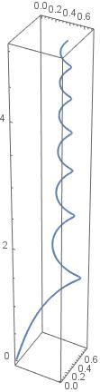
Figure 1: Motion of an electric charge in a linear magnetic field along a fixed vector.

Let us now consider the motion of a dyon in this magnetic background by including an axial electric field $\vec{E}=(0,0,\varrho\,z)$, with $e\,\varrho>0$, which yields a harmonic force corresponding to a confining potential $V=\frac{e\,\varrho}{2}\,z^{2}$ in the $z$-direction. In this case the time evolution of the axial position coordinate with the initial conditions $z(0)=0$ and $\dot{z}(0)=v_{z}$ is given by $z(t)=v_{z}\sin(\varpi\,t)/\varpi$, with oscillation frequency $\varpi=\sqrt{2\,e\,\varrho/m}$. The differential equation for the kinematical momentum $2\,{\tilde{\pi}}_{y}$ then becomes

$$\ddot{\tilde{\pi}}_{y}-\varpi\cot(\varpi\,t)\,\dot{\tilde{\pi}}_{y}+\mbox{$\frac{\omega^{2}\,v_{z}^{2}}{\varpi^{2}}$}\sin^{2}(\varpi\,t)\,{\tilde{\pi}}_{y}=0\ ,$$ (6.15)

which reduces to (6.12) in the limit $\varrho=0$. For the special electric charge density $\varrho=m/2e$, i.e. $\varpi=1$, the appropriate choice of initial data gives the solutions

$${\tilde{\pi}}_{x}(t)=\cos(\omega\,v_{z}\cos t)\qquad\mbox{and}\qquad{\tilde{\pi}}_{y}(t)=\sin(\omega\,v_{z}\cos t)\ .$$ (6.16)

By electromagnetic duality, we should also set the magnetic charge density to $\rho=m/2e$, i.e. $\omega=1/2$. Since $\cos\big{(}\frac{v_{z}}{2}\cos t\big{)}\geq\cos\big{(}\frac{v_{z}}{2}\big{)}>0$ if $v_{z}\leq 3$, the position coordinate $x(t)$ then increases monotonically with time, so that the motion deconfines in the $(x,y)$-plane after confining the motion along the $z$-direction. That is, the three-dimensional motion cannot be completely confined, contrary to the expectations of [13]. This suggests that the corresponding quantum Hamiltonian exhibits a continuous energy spectrum. Below we shall investigate various aspects of the quantum mechanics of electric charge in the monopole background within our symplectic realisation.

Finally, we look at the dynamics of the auxiliary coordinates. With the physical solution (6.13), from (3.10) they evolve according to the equations of motion

$$\dot{\pi}_{x} = \omega\,v_{z}\,\big{(}t\,{\pi}_{y}+\mbox{$\frac{m}{2}$}\,\tilde{y}-\mbox{$\frac{m\,v_{y}}{2}$}\,t\cos(\mbox{$\frac{\omega\,v_{z}}{2}$}\,t^{2})\big{)}\ ,$$

$$\dot{\pi}_{y} = -\omega\,v_{z}\,\big{(}t\,{\pi}_{x}+\mbox{$\frac{m}{2}$}\,\tilde{x}-\mbox{$\frac{m\,v_{y}}{2}$}\,t\sin(\mbox{$\frac{\omega\,v_{z}}{2}$}\,t^{2})\big{)}\ ,$$

$$\dot{\pi}_{z} = \mbox{$\frac{m\,\omega\,v_{y}}{2}$}\,\big{(}\cos(\mbox{$\frac{\omega\,v_{z}}{2}$}\,t^{2})\,\tilde{x}-\sin(\mbox{$\frac{\omega\,v_{z}}{2}$}\,t^{2})\,\tilde{y}\big{)}\ .$$ (6.17)

Thus the auxiliary degrees of freedom obey a complicated inhomogeneous system of coupled differential equations, which we have not been able to integrate; it would be interesting to better understand the physical significance of the auxiliary coordinates from these equations. This is in marked contrast to the case of a uniform magnetic field $\vec{B}$, whereby (3.10) would yield precisely the same Lorentz force law for the auxiliary variables, as expected since in that case the constraints (4.1) and (4.5) can be consistently imposed.

This example illustrates that the symplectic realisation is not always necessary for the integrability of the classical motion. However, it is necessary for a proper formulation of geometric quantisation, i.e. for a description of the “canonical” quantum mechanics. This is analogous to the situation of an electric charge in the background of a Dirac monopole, wherein the classical equations of motion can be integrated without an action formalism, but for quantisation it is necessary to construct a suitable vector potential in order to define a Hamiltonian.

7 Quantum dynamics from symplectic realisation

In this section we describe the quantisation of the dynamical system with Poisson brackets (2.10) and Hamiltonian (3.11). We shall mostly ignore the electric background in our discussion and set the scalar potential to $V=0$. In the Schrödinger polarisation, the quantum Hilbert space $\mathscr{H}=L^{2}({\mathbb{R}}^{6})$ consists of square-integrable wavefunctions $\Psi$ (with respect to the standard Lebesgue measure) on the extended configuration space of the charged particle, which later on we will treat geometrically as sections of the trivial line bundle over ${\mathbb{R}}^{6}$ with connection $A_{I}$. On $\mathscr{H}$ we represent position operators $\widehat{x}{}^{I}$ as multipliers, $\big{(}\widehat{x}{}^{I}\Psi\big{)}(x)=x^{I}\,\Psi(x)$ with $x^{I}=(x^{i},\tilde{x}^{i})$, and the canonical momentum operators $\widehat{p}_{I}$ as derivatives, $\big{(}\widehat{p}_{I}\Psi\big{)}(x)=-{\,{\rm i}\,}\hbar\,\partial_{I}\Psi(x)$ with $\partial_{I}=(\partial_{i},\tilde{\partial}_{i})$. Then the kinematical momentum operators

$$\widehat{\pi}_{I}=\big{(}\widehat{\pi}_{i},\widehat{\tilde{\pi}}_{i}\big{)}=-{\,{\rm i}\,}\hbar\,\partial_{I}-e\,A_{I}$$ (7.1)

define covariant differentiation on the trivial line bundle.

The corresponding quantum Hamiltonian is

$$\widehat{{\mathcal{H}}}=\mbox{$\frac{1}{m}$}\,\widehat{\pi}_{I}\,\eta^{IJ}\,\widehat{\pi}_{J}=\mbox{$\frac{1}{m}$}\,\big{(}\widehat{\pi}_{i}\,\widehat{\tilde{\pi}}{}^{i}+\widehat{\tilde{\pi}}_{i}\,\widehat{\pi}{}^{i}\big{)}=\mbox{$\frac{2}{m}$}\,\big{(}-{\,{\rm i}\,}\hbar\,\vec{\nabla}-e\,\vec{A}\,\big{)}\cdot\big{(}-{\,{\rm i}\,}\hbar\,\vec{\tilde{\nabla}}-e\,\vec{\tilde{A}}\,\big{)}\ .$$ (7.2)

The probability current $\mathcal{J}^{I}=(\mathcal{J}^{i},\tilde{\mathcal{J}}{}^{i})$ for a given state $\Psi$ is defined by

$$\mathcal{J}^{I}=\mbox{$\frac{1}{m}$}\,\big{(}(\Psi^{\ast}\,\eta^{IJ}\,\widehat{p}_{J}\Psi-\Psi\,\eta^{IJ}\,\widehat{p}_{J}\Psi^{\ast})-2\,e\,\eta^{IJ}\,A_{J}\,|\Psi|^{2}\big{)}\ .$$ (7.3)

Since the energy is conserved, as we have discussed in Section 6, it suffices to consider stationary states $\Psi$ which vary simply with a time-dependent phase and we can study energy eigenvalues ${\mathcal{E}}$ of the quantum Hamiltonian (7.2) via the time-independent Schrödinger equation

$$\widehat{{\mathcal{H}}}\Psi={\mathcal{E}}\,\Psi\ .$$ (7.4)

Due to (7.4), in a stationary state the probability current is conserved,

$$\partial_{I}\mathcal{J}^{I}=0\ ,$$ (7.5)

and hence the quantum theory is also unitary.

This quantum theory is defined on a six-dimensional configuration space $(x^{i},\tilde{x}^{i})$. In particular, the probability current also has six components. Just as in the classical situation considered in Section 4, we can try to eliminate the auxiliary degrees of freedom via quantum Hamiltonian reduction by imposing the constraints (4.1) and (4.5) (with $\zeta=\gamma=1$) at the quantum level, i.e. by restricting to the subspace $\mathscr{H}_{\rm phys}\subset\mathscr{H}$ of physical states $\Psi_{\rm phys}$ which are annihilated by the constraint operators:

$$\widehat{\phi}{}^{\,i}\Psi_{\rm phys}=\big{(}\,\widehat{\tilde{x}}{}^{\,i}-\widehat{x}{}^{\,i}\big{)}\Psi_{\rm phys}=0\qquad\mbox{and}\qquad\widehat{\psi}{}_{i}\Psi_{\rm phys}=\big{(}\,\widehat{\tilde{\pi}}{}_{i}-\widehat{\pi}{}_{i}\big{)}\Psi_{\rm phys}=0\ .$$ (7.6)

The relevant commutator to analyse is given by

$$\big{[}\,\widehat{\tilde{\pi}}_{i},\widehat{\pi}_{j}\big{]}=\big{[}\widehat{\pi}_{i},\widehat{\tilde{\pi}}_{j}\big{]}=\mbox{$\frac{{\,{\rm i}\,}\hbar\,e}{2}$}\,\varepsilon_{ijk}\,\widehat{B}{}^{k}\ ,$$ (7.7)

where $\widehat{B}{}^{k}$ is the multiplier by the magnetic field $\vec{B}(\vec{x}\,)$.

If the magnetic field $\vec{B}$ is divergenceless, i.e. $\vec{B}=\vec{\nabla}\times\vec{a}$ everywhere, then the vector potential $A_{I}(x^{I})$ can be defined as

$$\vec{A}(x^{I})=\mbox{$\frac{1}{2}$}\,\big{(}\vec{a}(\vec{x}\,)-(\vec{x}\cdot\vec{\nabla})\vec{a}(\vec{x}\,)-\vec{\tilde{x}}\times\vec{B}(\vec{x}\,)\big{)}\qquad\mbox{and}\qquad\vec{\tilde{A}}(x^{I})=\vec{0}\ .$$ (7.8)

With this choice, the effective quantum theory after resolving the constraints (7.6) coincides with the standard quantum mechanical description of a charged particle in the magnetic field with the Hamiltonian

$$\widehat{{\mathcal{H}}}_{\rm eff}=\mbox{$\frac{1}{2m}$}\,\widehat{\pi}_{i}\,\widehat{\pi}^{\,i}\ ,$$ (7.9)

where

$$\big{[}\widehat{\pi}_{i},\widehat{\pi}_{j}\big{]}={\,{\rm i}\,}\hbar\,e\,\varepsilon_{ijk}\,\widehat{B}{}_{\rm eff}^{k}={\,{\rm i}\,}\hbar\,e\,\big{(}\widehat{\partial_{i}a_{j}}-\widehat{\partial_{j}a_{i}}\big{)}\ .$$ (7.10)

In situations where the vector field $\vec{a}(\vec{x}\,)$ is not globally defined on $\mathbb{R}^{3}$ but only in specified compact regions, like in the case of the Dirac monopole, one can excise the support of the magnetic charge distribution $\vec{\nabla}\cdot\vec{B}$ from the configuration space and take the wavefunctions to be sections of a corresponding non-trivial line bundle over the excised space of degree $n\in{\mathbb{Z}}$ given by the Dirac charge quantisation condition (6.9) [51]. In the standard treatments one needs to restrict the domains of quantum operators to wavefunctions which vanish sufficiently fast on the Dirac string, whereas in our approach we can simply consider wavefunctions in $\mathscr{H}_{\rm phys}=L^{2}({\mathbb{R}}^{3})$ that vanish at the locus of the magnetic charge distribution, which provides a suitable extension of the effective Hamiltonian (7.9) to an essentially self-adjoint operator on $\mathscr{H}_{\rm phys}$ [4]. It is known that a Dirac monopole and an electric charge do not form a bound state, whereas dyonic bound states are possible [54].

However, if $\vec{\nabla}\cdot\vec{B}\neq 0$ everywhere then a vector potential $\vec{a}(\vec{x}\,)$ does not exist even locally and the effective magnetic field in (7.10) does not account for the contribution from magnetic sources. In particular, for the spherically symmetric magnetic field (2.15) it simply vanishes, $\vec{B}_{\rm eff}=\vec{0}$, and thus in this case the constraints (7.6) lead to a free particle quantum theory without any interaction with the magnetic field.

To understand better the quantum theory described by the Hamiltonian (7.2), we first observe that it is an unbounded operator on $\mathscr{H}$. It is convenient to represent it as a difference of two Hamiltonians which are each bounded from below as

$$\widehat{{\mathcal{H}}}=\widehat{{\mathcal{H}}}_{+}-\widehat{{\mathcal{H}}}_{-}:=\mbox{$\frac{1}{m}$}\,\widehat{\pi}{}_{i\,+}\,\widehat{\pi}^{\,i}_{+}-\mbox{$\frac{1}{m}$}\,\widehat{\pi}{}_{i\,-}\,\widehat{\pi}^{\,i}_{-}\ ,$$ (7.11)

where

$$\widehat{\pi}{}_{i\,\pm}=\mbox{$\frac{1}{\sqrt{2}}$}\,\big{(}\widehat{\pi}_{i}\pm\widehat{\tilde{\pi}}_{i}\big{)}\ .$$ (7.12)

The pairs of kinematical momentum operators (7.12) do not commute in general,

$$\big{[}\widehat{\pi}{}_{i\,+},\widehat{\pi}{}_{j\,-}\big{]}=\mbox{$\frac{{\,{\rm i}\,}\hbar\,e}{2}$}\,\big{(}\varepsilon_{ijk}\,\widehat{\partial_{l}B^{k}}-\varepsilon_{ijl}\,\widehat{\partial_{k}B^{k}}\big{)}\,\widehat{\tilde{x}}{}^{\,l}\ ,$$ (7.13)

and consequently neither do the Hamiltonians $\widehat{{\mathcal{H}}}_{+}$ and $\widehat{{\mathcal{H}}}_{-}$ unless the magnetic field is constant. Let us begin by considering some typical examples which illustrate how the imposition of the constraints (7.6) recovers well-known results, before moving on to our main examples of interest with smooth distributions of magnetic charge.

Free particle.   As a warmup, let us see how to reproduce free particle quantum states in the absence of a magnetic field, $A_{I}=0$. The Schrödinger equation (7.4) in this case is

$$-\frac{2\hbar^{2}}{m}\,\vec{\nabla}\cdot\vec{\tilde{\nabla}}\Psi(\vec{x},\vec{\tilde{x}}\,)={\mathcal{E}}\,\Psi(\vec{x},\vec{\tilde{x}}\,)\ .$$ (7.14)

The eigenfunctions are the plane waves

$$\Psi_{\vec{k},\vec{\tilde{k}}}(\vec{x},\vec{\tilde{x}}\,)={\,\rm e}\,^{-\frac{{\,{\rm i}\,}}{2\hbar}\,(\vec{k}\cdot\vec{x}+\vec{\tilde{k}}\cdot\vec{\tilde{x}}\,)}\ ,$$ (7.15)

with eigenvalues

$${\mathcal{E}}_{\vec{k},\vec{\tilde{k}}}=\frac{\vec{k}\cdot\vec{\tilde{k}}}{2m}\ .$$ (7.16)

The physical state conditions (7.6) then force $\vec{x}=\vec{\tilde{x}}$ and $\vec{k}=\vec{\tilde{k}}$, yielding the expected free particle plane waves and kinetic energy spectrum

$$\Psi_{\rm phys}(\vec{x}\,)=\Psi_{\vec{k},\vec{k}}(\vec{x},\vec{x}\,)={\,\rm e}\,^{-\frac{{\,{\rm i}\,}}{\hbar}\,\vec{k}\cdot\vec{x}}\qquad\mbox{and}\qquad E_{\vec{k}}={\mathcal{E}}_{\vec{k},\vec{k}}=\frac{\vec{k}^{\,2}}{2m}\ .$$ (7.17)

Landau levels.   Consider the Landau problem, i.e. the motion of an electric charge in a constant and uniform magnetic field $\vec{B}$, which by a suitable choice of coordinates we can take to lie along the $z$-axis, $\vec{B}=(0,0,B)$. In this case

$$\vec{A}(x^{I})=\mbox{$\frac{B}{2}$}\,(-\tilde{y},\tilde{x},0)\qquad\mbox{and}\qquad\vec{\tilde{A}}(x^{I})=\vec{0}\ ,$$ (7.18)

and the only non-vanishing commutators between the covariant momentum operators are given by

$$\big{[}\widehat{\pi}{}_{x\,\pm},\widehat{\pi}{}_{y\,\pm}\big{]}=\pm{\,{\rm i}\,}\hbar\,e\,B\ .$$ (7.19)

In particular, the axial momentum operators $\widehat{p}_{z}$ and $\widehat{\tilde{p}}_{z}$ commute with all other momentum operators, and so the quantum states in the direction of $\vec{B}$ decouple into free particle states which can be solved for along the same lines as above. Henceforth we therefore consider only the planar quantum states and, assuming $e\,B>0$, we introduce creation and annihilation operators as

$$\widehat{a}_{\pm}=\mbox{$\frac{1}{\sqrt{2\,\hbar\,e\,B}}$}\,\big{(}\widehat{\pi}{}_{x\,\pm}+{\,{\rm i}\,}\widehat{\pi}{}_{y\,\pm}\big{)}\qquad\mbox{and}\qquad\widehat{a}{}^{\dagger}_{\pm}=\mbox{$\frac{1}{\sqrt{2\,\hbar\,e\,B}}$}\,\big{(}\widehat{\pi}{}_{x\,\pm}-{\,{\rm i}\,}\widehat{\pi}{}_{y\,\pm}\big{)}\ .$$ (7.20)

One easily checks

$$\big{[}\widehat{a}_{\pm},\widehat{a}{}^{\dagger}_{\pm}\big{]}=1\ ,$$ (7.21)

while all other commutators vanish.

In terms of the operators (7.20) the Hamiltonian (7.11) can be written as

$$\widehat{{\mathcal{H}}}=\widehat{{\mathcal{H}}}_{+}-\widehat{{\mathcal{H}}}_{-}:=\hbar\,\omega_{\rm cyc}\,\big{(}\widehat{a}{}^{\dagger}_{+}\,\widehat{a}_{+}-\widehat{a}{}^{\dagger}_{-}\,\widehat{a}_{-}-1\big{)}\ ,$$ (7.22)

where

$$\omega_{\rm cyc}=\frac{e\,B}{m}$$ (7.23)

is the cyclotron frequency. This Hamiltonian is unbounded, but it can be decomposed into the difference of two Hamiltonians $\widehat{{\mathcal{H}}}_{\pm}$ of harmonic oscillator type which are bounded from below and commute, $\big{[}\widehat{{\mathcal{H}}}_{+},\widehat{{\mathcal{H}}}_{-}\big{]}=0$. As discussed in Appendix B, the simultaneous eigenvalues of $\widehat{a}{}^{\dagger}_{\pm}\,\widehat{a}_{\pm}$ are the integers $n_{\pm}\in{\mathbb{N}}_{0}$ such that the eigenvalues of (7.22) are

$${\mathcal{E}}_{n_{+},n_{-}}=\hbar\,\omega_{\rm cyc}\,(n_{+}-n_{-}-1)$$ (7.24)

with corresponding eigenstates $|n_{+},n_{-}\rangle$ in the standard number basis for the two-particle bosonic Fock space $\mathscr{F}$. Using the definition of the annihilation operator $\widehat{a}_{-}$ from (7.20), the physical state constraints (7.6) read $\widehat{a}_{-}\Psi_{\rm phys}=0$, which implies that the $\widehat{a}_{-}$-oscillator must be kept in its ground state for which $\widehat{a}_{-}|n_{+},0\rangle=0$. Then the standard harmonic oscillator spectrum $E_{n}={\mathcal{E}}_{n,0}$, and hence the Landau levels of the electric charge, emerge. This is the same as the known constraint from the quantum theory of dissipative dynamics [26, 20, 18, 30], see Appendix B.

Axial magnetic fields.   The natural extension of the Landau problem considered above is to the motion of an electric charge in a constant and uniform magnetic charge distribution which sources an axial magnetic field (2.18). In this case the vector potential is given by (4.20) and the Hamiltonian reads

$$\widehat{{\mathcal{H}}}=\mbox{$\frac{1}{m}$}\,\big{(}\widehat{\pi}{}^{2}_{x\,+}+\widehat{\pi}{}^{2}_{y\,+}\big{)}-\mbox{$\frac{1}{m}$}\,\big{(}\widehat{\pi}{}^{2}_{x\,-}+\widehat{\pi}{}^{2}_{y\,-}\big{)}+\mbox{$\frac{2}{m}$}\,\widehat{p}_{z}\,\widehat{\tilde{p}}_{z}\ ,$$ (7.25)

with the algebra of non-vanishing commutation relations among momentum operators given by

$$\big{[}\widehat{\pi}_{x\,\pm},\widehat{\pi}_{y\,\pm}\big{]} = \pm\,\mbox{$\frac{{\,{\rm i}\,}\hbar}{4}$}\,e\,\rho\,\widehat{z}\ ,$$

$$\big{[}\widehat{\pi}_{x\,\pm},\widehat{p}_{z}\big{]} = \pm\,\mbox{$\frac{{\,{\rm i}\,}\hbar}{4\,\sqrt{2}}$}\,e\,\rho\,\big{(}\,\widehat{y}-2\,\widehat{\tilde{y}}\,\big{)}\ ,$$

$$\big{[}\widehat{\pi}_{y\,\pm},\widehat{p}_{z}\big{]} = \pm\,\mbox{$\frac{{\,{\rm i}\,}\hbar}{4\,\sqrt{2}}$}\,e\,\rho\,\big{(}\,2\,\widehat{\tilde{x}}-\widehat{x}\,\big{)}\ .$$ (7.26)

In particular $\big{[}\widehat{{\mathcal{H}}},\widehat{\tilde{p}}_{z}\big{]}=0$, so the quantum states form representations of the translation group generated by $\widehat{p}_{z}$, which are superpositions of the simultaneous eigenstates of the axial momentum operator given by

$$\Psi_{\tilde{p}_{z}}\big{(}\vec{x},\vec{\tilde{x}}\,\big{)}={\,\rm e}\,^{{\,{\rm i}\,}\tilde{p}_{z}\,\tilde{z}/\hbar}\ \Psi(x,y,z,\tilde{x},\tilde{y})\qquad\mbox{with}\quad\widehat{\tilde{p}}_{z}\Psi_{\tilde{p}_{z}}=\tilde{p}_{z}\,\Psi_{\tilde{p}_{z}}\ .$$ (7.27)

This defines a decomposition of the quantum Hilbert space $\mathscr{H}$ into a direct integral $\int^{\oplus}_{\tilde{p}_{z}\in{\mathbb{R}}}\,\mathscr{H}_{\tilde{p}_{z}}:=L^{2}({\mathbb{R}},\mathscr{H})$, the square-integrable sections of the state space viewed as a (trivial) Hilbert bundle over the line ${\mathbb{R}}$ of axial momenta. The Schrödinger equation (7.4) in the fiber subspace over $\tilde{p}_{z}\in{\mathbb{R}}$ is equivalent to $\widehat{{\mathcal{H}}}_{\tilde{p}_{z}}\Psi={\mathcal{E}}\,\Psi$, with the restriction of the Hamiltonian $\widehat{{\mathcal{H}}}_{\tilde{p}_{z}}:=\widehat{{\mathcal{H}}}\big{|}_{\mathscr{H}_{\tilde{p}_{z}}}$ given by

$$\widehat{{\mathcal{H}}}_{\tilde{p}_{z}}=\mbox{$\frac{1}{m}$}\,\big{(}\widehat{\pi}{}^{2}_{x\,+}+\widehat{\pi}{}^{2}_{y\,+}\big{)}-\mbox{$\frac{1}{m}$}\,\big{(}\widehat{\pi}{}^{2}_{x\,-}+\widehat{\pi}{}^{2}_{y\,-}\big{)}+\mbox{$\frac{2}{m}$}\,\tilde{p}_{z}\ \widehat{p}_{z}\ .$$ (7.28)

Let us now introduce the frequency

$$\omega=\frac{e\,\rho}{m}$$ (7.29)

which appears in the classical solution of Section 6, and we assume again that $e\,\rho>0$. We further introduce the “creation” and “annihilation” operators

$$\widehat{a}_{\pm}=\sqrt{\mbox{$\frac{2}{\hbar\,m\,\omega}$}}\ \big{(}\widehat{\pi}_{x\,\pm}+{\,{\rm i}\,}\widehat{\pi}_{y\,\pm}\big{)}\qquad\mbox{and}\qquad\widehat{a}{}^{\dagger}_{\pm}=\sqrt{\mbox{$\frac{2}{\hbar\,m\,\omega}$}}\ \big{(}\widehat{\pi}_{x\,\pm}-{\,{\rm i}\,}\widehat{\pi}_{y\,\pm}\big{)}\ ,$$ (7.30)

with the non-vanishing commutation relations

$$\big{[}\widehat{a}_{\pm},\widehat{a}{}^{\dagger}_{\pm}\big{]}=\widehat{z}\ .$$ (7.31)

In particular, the axial position operator $\widehat{z}$ is central in this “oscillator” algebra: $\big{[}\widehat{a}_{\pm},\widehat{z}\big{]}=0$ and $\big{[}\widehat{a}{}^{\dagger}_{\pm},\widehat{z}\big{]}=0$. One easily checks the further non-vanishing commutators

$$\big{[}\widehat{a}_{\pm},\widehat{p}_{z}\big{]}=\mp\,\sqrt{\mbox{$\frac{\hbar}{m\,\omega}$}}\ \mbox{$\frac{e}{2}$}\ \widehat{w}\qquad\mbox{and}\qquad\big{[}\widehat{a}{}^{\dagger}_{\pm},\widehat{p}_{z}\big{]}=\pm\,\sqrt{\mbox{$\frac{\hbar}{m\,\omega}$}}\ \mbox{$\frac{e}{2}$}\ \widehat{w}{}^{\dagger}\ ,$$ (7.32)

where

$$\widehat{w}=\big{(}\,\widehat{\tilde{x}}+{\,{\rm i}\,}\widehat{\tilde{y}}\,\big{)}-\mbox{$\frac{1}{2}$}\,\big{(}\widehat{x}+{\,{\rm i}\,}\widehat{y}\big{)}\qquad\mbox{and}\qquad\widehat{w}{}^{\dagger}=\big{(}\,\widehat{\tilde{x}}-{\,{\rm i}\,}\widehat{\tilde{y}}\,\big{)}-\mbox{$\frac{1}{2}$}\,\big{(}\widehat{x}-{\,{\rm i}\,}\widehat{y}\big{)}\ ,$$ (7.33)

and of course one has the canonical commutator

$$\big{[}\widehat{z}\,,\,\widehat{p}_{z}\big{]}={\,{\rm i}\,}\hbar\ .$$ (7.34)

The Hamiltonian (7.28) then becomes

$$\widehat{{\mathcal{H}}}_{\tilde{p}_{z}}=\mbox{$\frac{\hbar}{2}$}\,\omega\,\big{(}\widehat{a}{}^{\dagger}_{+}\,\widehat{a}_{+}-\widehat{a}{}^{\dagger}_{-}\,\widehat{a}_{-}-\widehat{z}\big{)}+\mbox{$\frac{2}{m}$}\,\tilde{p}_{z}\ \widehat{p}_{z}\ .$$ (7.35)

Naively, this Hamiltonian resembles that of the Landau problem considered above, in that it decomposes into a free particle Hamiltonian in the axial direction plus a doubled “oscillator” system in the planar directions. However, due to (7.32) and (7.34), these two components do not commute, and moreover the planar “oscillator” depends explicitly on the axial position operator through (7.31). This coupling between the planar and axial momentum operators hinders a complete analytic solution of the Schrödinger equation, in contrast to the classical dynamics from Section 6 where the free motion in the axial direction effectively reduces the problem to planar motion in a time-dependent magnetic field which we were able to integrate. Note that on physical states $\Psi_{\rm phys}$ satisfying the analogue of the constraint equations (7.6) with $\zeta=\frac{1}{2}$ in (4.1) one has $\widehat{w}\Psi_{\rm phys}=0=\widehat{w}{}^{\dagger}\Psi_{\rm phys}$, so that the planar and axial Hamiltonians commute on $\mathscr{H}_{\rm phys}$, but now additionally $\widehat{a}_{+}\Psi_{\rm phys}=0=\widehat{a}_{-}\Psi_{\rm phys}$ from (7.6) so that the planar quantum dynamics trivialises and the free particle axial states follow as before.

For states with vanishing axial momentum $\tilde{p}_{z}=0$, the spectrum of the Hamiltonian

$$\widehat{{\mathcal{H}}}_{0}=\mbox{$\frac{\hbar}{2}$}\,\omega\,\big{(}\widehat{a}{}^{\dagger}_{+}\,\widehat{a}_{+}-\widehat{a}{}^{\dagger}_{-}\,\widehat{a}_{-}-\widehat{z}\big{)}$$ (7.36)

is readily obtained: Via Fourier transformation of the Schrödinger polarisation, we can represent the axial position operator as the derivative $\widehat{z}={\,{\rm i}\,}\hbar\,\frac{\partial}{\partial p_{z}}$ so that the subspace $\mathscr{H}_{0}=\mathscr{F}\otimes L^{2}({\mathbb{R}})$ is spanned by the eigenstates

$$\Psi^{(0)}_{n_{+},n_{-};z}(p_{z})=|n_{+},n_{-}\rangle\otimes\psi_{z}(p_{z})$$ (7.37)

of (7.36), where $\psi_{z}(p_{z})={\,\rm e}\,^{-{\,{\rm i}\,}z\,p_{z}/\hbar}$ are the eigenstates of $\widehat{z}$ with axial position eigenvalue $z\in{\mathbb{R}}$. The correponding energy eigenvalues are

$${\mathcal{E}}^{(0)}_{n_{+},n_{-};z}=\mbox{$\frac{\hbar}{2}$}\,\omega\,z\,\big{(}n_{+}-n_{-}-1\big{)}\ ,$$ (7.38)

which is the spectrum of a doubled harmonic oscillator with an axial position-dependent frequency. For small momenta, via a suitable (length) regularisation of the inner product on $L^{2}({\mathbb{R}})$ it is easy to see that the first order correction to these energies due to the perturbation by the axial momentum operator in (7.35) vanishes, so that (7.38) represents the energy of the system up to order $O\big{(}\tilde{p}{}^{2}_{z}\big{)}$. Thus the quantum dynamics of the electric charge in an axial magnetic field exhibits a continuous energy spectrum, and by our calculations from Section 6 we do not expect the situation to change by inclusion of a corresponding axial electric field.

It would be interesting to find the exact spectrum of the Hamiltonian (7.35), but we will content ourselves here with the approximate solution (7.38). The situation is of course much more complicated for the spherically symmetric magnetic field (2.15), whose dyonic classical Hamiltonian is given by (5.15), due to the fact that fewer integrals of motion exist in that case. In Sections 8 and 9 below we shall discuss some of the features of the charged particle wavefunctions in the spherically symmetric case.

8 Extended magnetic translations and two-cocycles

One of the most interesting aspects of the quantum dynamics of electric charge in magnetic backgrounds is the physical and mathematical structure of the magnetic translation group [53]. For source-free magnetic fields, the electron wavefunctions carry a (weak) projective representation of the translation group ${\mathbb{R}}^{3}$ whose two-cocycle is defined by the magnetic flux. On the other hand, for magnetic fields sourced by monopole distributions, the representation of the translation group is obstructed by an anomalous three-cocycle defined by the magnetic charge, which encodes a “nonassociative representation” in the sense that the parallel transports implementing the translations do not associate [31]; in this case one cannot assign operators to the translation generators which act on a separable Hilbert space and one is forced to deal with other methods of quantisation, such as the phase space formulation of nonassociative quantum mechanics [42, 48], or the action of parallel transports on a 2-Hilbert space which generates higher projective representations [14]. In this section we wish to see how these obstructing three-cocycles are captured within the associative framework of our symplectic realisation, following the treatment of magnetic translations from [28, 47] which we adapt to our situation.

The key feature of the symplectic realisation is the existence of a globally defined vector potential (2.8), which we interpret geometrically as a connection on the trivial line bundle over ${\mathbb{R}}^{6}$. Gauge invariance of the Schrödinger equation (7.4) dictates that a gauge transformation $A_{I}\mapsto A_{I}+\partial_{I}\chi$ is accompanied by a corresponding phase transformation $\Psi\mapsto{\,\rm e}\,^{{\,{\rm i}\,}e\,\chi}\,\Psi$ of the electron wavefunctions $\Psi\in\mathscr{H}$. In the presence of the magnetic field $\vec{B}(\vec{x}\,)$, the translation generators $\partial_{I}$ on the extended configuration space ${\mathbb{R}}^{6}$ are modified to the kinematical momentum operators (7.1), and hence we must extend the natural operators which generate translations by vectors $r=(\vec{r},\vec{\tilde{r}}\,)\in{\mathbb{R}}^{6}$ on the quantum Hilbert space $\mathscr{H}=L^{2}({\mathbb{R}}^{6})$ to magnetic translation operators $\widehat{T}{}(r)$ which act on wavefunctions $\Psi\in\mathscr{H}$ at a point $x\in{\mathbb{R}}^{6}$ by parallel transport along the line connecting $x$ to $x+r$:

$$\big{(}\widehat{T}{}(r)\Psi\big{)}(x)=\exp\Big{(}\,\frac{{\,{\rm i}\,}e}{\hbar}\,\int_{0}^{1}\,{\rm d}t\ r^{I}\,A_{I}(x+t\,r)\,\Big{)}\,\Psi(x+r)\ .$$ (8.1)

This defines a one-cochain of the translation group in six dimensions.

The operator $\widehat{T}{}(r)\,\widehat{T}{}(s)\,\widehat{T}{}(r+s)^{-1}$ performs the parallel transport of the wavefunction $\Psi(x)$ around the loop forming the boundary $\partial\triangle(x;r,s)$ of the triangle $\triangle(x;r,s)$ based at $x\in{\mathbb{R}}^{6}$ and spanned by the translation vectors $r,s$. In terms of the one-form $A=A_{I}\,{\rm d}x^{I}=\vec{A}(\vec{x},\vec{\tilde{x}}\,)\cdot{\rm d}\vec{x}$ on the extended configuration space whose components are given by (2.8), this has the effect of multiplying $\Psi(x)$ by the Wilson loop $W(x;r,s)$ of the gauge field $\frac{e}{\hbar}\,A$ around $\partial\triangle(x;r,s)$. We then obtain the relations

$$\widehat{T}{}(r)\,\widehat{T}{}(s)=\widehat{\Omega}(r,s)\,\widehat{T}{}(r+s)\ ,$$ (8.2)

where the mutually commuting quantum operators $\widehat{\Omega}(r,s)$ for $r,s\in{\mathbb{R}}^{6}$ are the multipliers

$$\big{(}\widehat{\Omega}(r,s)\Psi\big{)}(x):=W(x;r,s)\,\Psi(x)\ .$$ (8.3)

The phase factor $W(x;r,s)$ is the coboundary of the one-cochain defined by the parallel transport (8.1) which reads as

$$W(x;r,s):=\exp\Big{(}\,\frac{{\,{\rm i}\,}e}{\hbar}\,\oint_{\partial\triangle(x;r,s)}\,A\,\Big{)}=\exp\Big{(}\,\frac{{\,{\rm i}\,}e}{\hbar}\,\int_{\triangle(x;r,s)}\,F\,\Big{)}\ ,$$ (8.4)

where $F={\rm d}A$ is the field strength of $A$ whose components are given by (2.7) and we have used Stokes’ theorem.

By construction the extended magnetic translation operators associate,

$$\big{(}\widehat{T}{}(r)\,\widehat{T}{}(s)\big{)}\,\widehat{T}{}(u)=\widehat{T}{}(r)\,\big{(}\widehat{T}{}(s)\,\widehat{T}{}(u)\big{)}\ ,$$ (8.5)

which implies that the multipliers of (8.2) satisfy the two-cocycle condition

$$\widehat{\Omega}(r,s)\,\widehat{\Omega}(r+s,u)={}^{r}{}\widehat{\Omega}(s,u)\,\widehat{\Omega}(r,s+u)\ ,$$ (8.6)

where ${}^{r}{}\widehat{\Omega}(s,u):=\widehat{T}{}(r)\,\widehat{\Omega}(s,u)\,\widehat{T}{}(r)^{-1}$ is the multiplier

$$\big{(}{}^{r}{}\widehat{\Omega}(s,u)\Psi\big{)}(x):=W(x+r;s,u)\,\Psi(x)\ .$$ (8.7)

The relations (8.2) and (8.6) imply that the map $r\mapsto\widehat{T}{}(r)$ defines a weak projective representation of the translation group ${\mathbb{R}}^{6}$ on the quantum Hilbert space of states $\mathscr{H}$, where by “weak” we mean that the projective phase is a multiplier by (8.4) which has a non-trivial dependence on position coordinates $x\in{\mathbb{R}}^{6}$ [47].

Using the Poisson algebra (2.10), it is easy to compute the phase factor (8.4) explicitly in terms of surface integrals over triangles in the extended configuration space to get

$$W(x;r,s) = \exp\bigg{[}\,\frac{{\,{\rm i}\,}e}{\hbar}\,\Big{(}\,\frac{1}{2}\,\int_{\triangle(\vec{x};\vec{r},\vec{\tilde{s}}\,)}\,\vec{B}\cdot{\rm d}\vec{S}+\frac{1}{2}\,\int_{\triangle(\vec{x};\vec{\tilde{r}},\vec{s}\,)}\,\vec{B}\cdot{\rm d}\vec{S}$$ (8.8)

$$\qquad\qquad\qquad+\,\int_{\triangle(\vec{x};\vec{r},\vec{s}\,)}\,\big{(}\vec{\nabla}\cdot\vec{B}\,\big{)}\,\vec{\tilde{x}}\cdot{\rm d}\vec{S}\,\Big{)}\,\bigg{]}\ .$$

The third integration can be expressed as a volume integral over the tetrahedron $\triangle(\vec{x};\vec{\tilde{x}},\vec{r},\vec{s}\,)$ based at $\vec{x}\in{\mathbb{R}}^{3}$ and spanned by the vectors $\vec{\tilde{x}},\vec{r},\vec{s}$. Altogether we then find

$$W(x;r,s)=\exp\bigg{[}\,\frac{{\,{\rm i}\,}e}{\hbar}\,\Big{(}\,\frac{1}{2}\,\int_{\triangle(\vec{x};\vec{r},\vec{\tilde{s}}\,)\cup\triangle(\vec{x};\vec{\tilde{r}},\vec{s}\,)}\,\vec{B}\cdot{\rm d}\vec{S}+\int_{\triangle(\vec{x};\vec{\tilde{x}},\vec{r},\vec{s}\,)}\,\vec{\nabla}\cdot\vec{B}\ {\rm d}V\,\Big{)}\,\bigg{]}\ .$$ (8.9)

The phase integrals in (8.9), which are each defined in terms of auxiliary coordinates, combine to give a hybrid of the usual magnetic flux two-cocycle in the source-free case and the magnetic charge three-cocycle in the presence of monopoles, in such a way so that $W(x;r,s)$ itself defines a two-cocycle of the extended translation group ${\mathbb{R}}^{6}$. Let us look at a few special cases to understand this structure more thoroughly.

We start with the source-free case, $\vec{\nabla}\cdot\vec{B}=0$, so that the second integral in (8.9) vanishes. As discussed in Section 7, in this instance one can consistently implement quantum Hamiltonian reduction through the constraints (7.6), and by restricting the action of the multipliers (8.3) to physical states $\Psi_{\rm phys}\in\mathscr{H}_{\rm phys}\subset\mathscr{H}$, one can identify physical and auxiliary translations and coordinates in (8.9) to get

$$W_{0}(\vec{x};\vec{r},\vec{s}\,)=\exp\Big{(}\,\frac{{\,{\rm i}\,}e}{\hbar}\,\int_{\triangle(\vec{x};\vec{r},\vec{s}\,)}\,\vec{B}\cdot{\rm d}\vec{S}\,\Big{)}\ .$$ (8.10)

Thus in this case we recover the standard two-cocycle of the anticipated (weak) projective representation of the translation group ${\mathbb{R}}^{3}$ [53].

Next, for the Dirac monopole field (2.4), by restricting to wavefunctions which vanish at the origin of ${\mathbb{R}}^{3}$ as discussed in Section 7, one may again impose the constraints (7.6), and hence identify physical and auxiliary variables in (8.9). The second integral now computes the magnetic charge enclosed by the tetrahedron $\triangle(\vec{x},\vec{r},\vec{s}\,)$, whose contribution to the phase is unity due to the Dirac charge quantisation condition (6.9). In this way we reproduce the result of [31] for the projective two-cocycle phase

$$W_{\rm D}(\vec{x};\vec{r},\vec{s}\,)=\exp\Big{(}\,\frac{{\,{\rm i}\,}e}{\hbar}\,\int_{\triangle(\vec{x};\vec{r},\vec{s}\,)}\,\vec{B}_{\rm D}\cdot{\rm d}\vec{S}\,\Big{)}$$ (8.11)

generated by the Dirac monopole.

Finally, let us consider the case of a constant magnetic charge distribution with spherically symmetric magnetic field (2.15). Contrary to the previous two cases, in this instance one cannot impose quantum Hamiltonian reduction to eliminate the auxiliary variables, and explicit computation of (8.9) yields

$$W_{\rm spher}(x;r,s)=\exp\bigg{[}\,\frac{{\,{\rm i}\,}e\,\rho}{\hbar}\,\Big{(}\,\frac{1}{6}\,\big{[}\vec{\tilde{r}},\vec{s},\vec{x}\,\big{]}+\frac{1}{6}\,\big{[}\vec{r},\vec{\tilde{s}},\vec{x}\,\big{]}+\big{[}\vec{r},\vec{s},\vec{\tilde{x}}\,\big{]}\,\Big{)}\,\bigg{]}\ ,$$ (8.12)

where the triple scalar product $\big{[}\vec{r},\vec{s},\vec{\tilde{x}}\,\big{]}:=\vec{r}\cdot\big{(}\vec{s}\times\vec{\tilde{x}}\,\big{)}$ is the volume of the tetrahedron $\triangle\big{(}\vec{r},\vec{s},\vec{\tilde{x}}\,\big{)}$ in the extended configuration space ${\mathbb{R}}^{6}$. The third phase contribution in (8.12) is the analogue of the three-cocycle of the translation group ${\mathbb{R}}^{3}$ which is calculated in nonassociative quantum mechanics [42, 48]; in the associative symplectic realisation, it is defined here by inserting an auxiliary position vector $\vec{\tilde{x}}$ into the third argument of the three-cocycle. Again, all three phase contributions together in (8.12) ensure a weak projective phase that defines a two-cocycle of the extended translation group ${\mathbb{R}}^{6}$.

In nonassociative quantum mechanics [42, 48], the non-trivial three-cocycle in the case of uniform magnetic charge density $\rho$ has profound physical consequences on the quantum system: It leads to a quantised momentum space with a quantum of minimal volume $\frac{1}{2}\,\hbar^{2}\,\rho$. In canonical (associative) quantum mechanics such volume quantisation is not observable, because there is no non-trivial volume operator. However, minimal areas are observable, such as the phase space Planck cell quantum $\hbar$, and for the present discussion the pertinent operator measuring area uncertainties in the extended momentum space is given by setting $\widehat{\bar{\pi}}_{\vec{r}}:=r^{i}\,\widehat{\bar{\pi}}_{i}$ for $\vec{r}\in{\mathbb{R}}^{3}$ and defining

$$\widehat{A}_{\vec{r},\vec{s}}:={\rm Im}\,\big{[}\,\widehat{\bar{\pi}}_{\vec{r}}\,,\,\widehat{\bar{\pi}}_{\vec{s}}\,\big{]}\ .$$ (8.13)

The idea behind this definition is that the vector product of two vectors $\vec{r},\vec{s}$ from the physical subspace is a vector in the extended configuration space, and so the operator $\widehat{A}_{\vec{r},\vec{s}}$ measures a physical volume in the extended space. Indeed, using the Poisson algebra (2.16), we may compute the expectation value of this oriented area operator in any state $\Psi\in\mathscr{H}$ (with the standard $L^{2}$-inner product) to get

$$\big{\langle}\Psi\big{|}\,\widehat{A}_{\vec{r},\vec{s}}\,\big{|}\Psi\big{\rangle}=\mbox{$\frac{\hbar\,e\,\rho}{3}$}\,\big{[}\vec{r},\vec{s},\delta_{\Psi}\vec{x}\,\big{]}\qquad\mbox{with}\quad\delta_{\Psi}x^{i}:=\big{\langle}\Psi\big{|}\,\widehat{\tilde{x}}{}^{\,i}-\widehat{x}{}^{\,i}\big{|}\Psi\big{\rangle}\ .$$ (8.14)

We have seen in this case that the quantum dynamics in magnetic charge backgrounds is not consistent with the physical state conditions (7.6), and hence the quantum tetrahedral volume computed by (8.14) is generically non-zero. This is the sense in which our associative formalism realises the characteristic minimal volumes. In Section 9 below we shall demonstrate more precisely the correspondence between the symplectic realisation and nonassociative quantum mechanics.

9 Nonassociative quantum mechanics

In this final section we shall conclude with somewhat more formal developments. One of our motivations for the present study was to understand the somewhat mysterious composition product that underlies the associative algebra of observables in nonassociative quantum mechanics [42], regarded as a nonassociative deformation of the standard phase space formulation of quantum mechanics [52], and provides an associative realisation of nonassociative star products. Deformation quantisation of the magnetic monopole algebra (2.1) was originally carried out via explicit construction of a nonassociative star product in [41] (see also [4, 36]), and cast into a quasi-Hopf algebraic framework in [42]. We shall demonstrate how the associative realisation of nonassociative quantum mechanics in terms of composition products from [42] can be realised explicitly in terms of an algebra of differential operators on phase space, and then show that this is identical to the quantum algebra given by the symplectic realisation of the underlying twisted Poisson structure.

Nonassociative star product.   For definiteness, throughout this section we work explicitly with a uniform monopole density of strength $\rho$ in three dimensions and the spherically symmetric magnetic field (2.15); the analysis can be generalised to non-constant magnetic charge distributions, at least perturbatively. For notational ease, we write the corresponding magnetic monopole algebra (2.1) collectively in terms of a twisted Poisson bivector $\theta$ on phase space $\mathcal{P}$ as

$$\{x^{a},x^{b}\}=\theta^{ab}(x)=\bigg{(}\begin{matrix}0&\delta^{i}{}_{j}\\ -\delta_{i}{}^{j}&\frac{e\,\rho}{3}\,\varepsilon_{ijk}\,x^{k}\end{matrix}\bigg{)}$$ (9.1)

where $x^{a}=(x^{i},\bar{\pi}_{i})$ with $i=1,2,3$ and $a=1,\dots,6$. The Jacobiator is given by

$$\Pi^{abc}=\{x^{a},x^{b},x^{c}\}=\bigg{(}\begin{matrix}0&0\\ 0&\frac{e\,\rho}{3}\,\varepsilon_{ijk}\end{matrix}\bigg{)}\ .$$ (9.2)

Deformation quantisation of the twisted Poisson structure is determined by the bidifferential operator

$${\cal F}=\exp\big{(}-\mbox{$\frac{{\,{\rm i}\,}\hbar}{2}$}\,\theta^{ab}(x)\,\partial_{a}\otimes\partial_{b}\big{)}\ ,$$ (9.3)

where $\partial_{a}=\frac{\partial}{\partial x^{a}}$, which defines a star product

$$f\star g:={\bm{\cdot}}\,{\cal F}\cdot(f\otimes g)$$ (9.4)

that is a noncommutative and nonassociative deformation of the pointwise product $f\,{\bm{\cdot}}\,g$ of smooth functions $f,g\in C^{\infty}(\mathcal{P})$. Various useful properties of this nonassociative star product can be found in [42, 36].

For constant monopole density, nonassociativity is controlled by the multiplicative associator

$$f\star(g\star h)=\Phi\big{(}(f\star g)\star h\big{)}:=\star\,\exp\big{(}-\mbox{$\frac{\hbar^{2}}{2}$}\,\Pi^{abc}\,\partial_{a}\otimes\partial_{b}\otimes\partial_{c}\big{)}\big{(}(f\otimes g)\otimes h\big{)}\ .$$ (9.5)

The twisted coproduct of a vector field $X$ on $\mathcal{P}$ is given by $\Delta(X)={\cal F}\,(X\otimes 1+1\otimes X)\,{\cal F}^{-1}$ [42]; it determines the deformed Leibniz rule

$$X(f\star g)=\star\,\Delta(X)(f\otimes g)\ .$$ (9.6)

In particular, the twisted coproduct of primitive translation generators is given by [42]

$$\Delta(\partial_{a})=\partial_{a}\otimes 1+1\otimes\partial_{a}+\mbox{$\frac{{\,{\rm i}\,}\hbar}{2}$}\,\Pi_{a}{}^{bc}\,\partial_{b}\otimes\partial_{c}$$ (9.7)

which yields the deformed Leibniz rule

$$\partial_{a}(f\star g)=(\partial_{a}f)\star g+f\star(\partial_{a}g)+\mbox{$\frac{{\,{\rm i}\,}\hbar}{2}$}\,\Pi_{a}{}^{bc}\,(\partial_{b}f)\star(\partial_{c}g)\ .$$ (9.8)

Composition product.   Recall the composition product $\circ$ from [42]: For functions $f,g,\varphi\in C^{\infty}(\mathcal{P})$, we define

$$(f\circ g)\star\varphi:=f\star(g\star\varphi)\ .$$ (9.9)

This defines a noncommutative product which is associative by construction, since by induction we have

$$(f_{1}\circ f_{2}\circ\cdots\circ f_{n})\star\varphi=f_{1}\star\big{(}f_{2}\star\big{(}\cdots\star(f_{n}\star\varphi)\cdots\big{)}\big{)}\ .$$ (9.10)

There is further a conjugate composition product $f\mathop{\bar{\circ}}g$ with the property $(f\circ g)^{*}=g^{*}\mathop{\bar{\circ}}f^{*}$ [42], but we shall not need it here. The associativity properties of the star product $\star$ are completely characterised by the composition products, in the sense that $\star$ is nonassociative if and only if there exist functions $f,g\in C^{\infty}(\mathcal{P})$ such that $f\circ g\notin C^{\infty}(\mathcal{P})$, while noncommutativity of the compositions themselves are characterised by the commutators $[f,g]_{\circ}:=f\circ g-g\circ f$. However, not all functions need have this property; for example, in the case of a constant monopole distribution $x^{a}\circ x^{a}=x^{a}\star x^{a}=x_{a}^{2}$; see [42] for details.

For constant monopole density we can explicitly characterise the subalgebra of differential operators ${\sf Diff}(\mathcal{P})$ on which the composition products close in terms of the star product $\star$. For this, we use the definition (9.9) and the associator relation (9.5) for arbitrary test functions $\varphi\in C^{\infty}(\mathcal{P})$ to find

$$f\circ g = f\star g$$

$$+\,\sum_{n=1}^{\infty}\,\frac{1}{n!}\,\Big{(}-\frac{\hbar^{2}}{2}\,\Big{)}^{n}\,\Pi^{a_{1}b_{1}c_{1}}\cdots\Pi^{a_{n}b_{n}c_{n}}\,\big{(}(\partial_{a_{1}}\cdots\partial_{a_{n}}f)\star(\partial_{b_{1}}\cdots\partial_{b_{n}}g)\big{)}\star\partial_{c_{1}}\cdots\partial_{c_{n}}$$

with $\partial_{a}\star\varphi:=\partial_{a}\varphi$. In particular, for the coordinate generators we find

$$[x^{a},x^{b}]_{\circ}={\,{\rm i}\,}\hbar\,\theta^{ab}(x)-\hbar^{2}\,\Pi^{abc}\,\partial_{c}\ .$$ (9.12)

From the deformed Leibniz rule (9.8) and the definition $(\partial_{a}\circ f)\star\varphi=\partial_{a}\star(f\star\varphi):=\partial_{a}(f\star\varphi)$ we have

$$\partial_{a}\circ f=\partial_{a}f+f\star\partial_{a}+\mbox{$\frac{{\,{\rm i}\,}\hbar}{2}$}\,\Pi_{a}{}^{bc}\,(\partial_{b}f)\star\partial_{c}\ .$$ (9.13)

The general relations in ${\sf Diff}(\mathcal{P})$ can be obtained as follows. We can extend the coproduct $\Delta$ to arbitrary differential operators $D=\sum_{k}\,d_{a_{1}\cdots a_{k}}(x)\,\partial_{a_{1}}\cdots\partial_{a_{k}}$ as an algebra homomorphism with $\Delta(1)=1\otimes 1$ and use the usual Sweedler notation (with implicit summation)

$$\Delta(D):=D_{(1)}\otimes D_{(2)}\ .$$ (9.14)

This encodes the deformed action of $D$ on star products $f\star\varphi$ and for any $f\in C^{\infty}(\mathcal{P})$ we have

$$D\circ f=(D_{(1)}\cdot f)\star D_{(2)}\ ,$$ (9.15)

while $f\circ D$ is given by the formula (9) with $g$ replaced by $D$ and the derivatives $\partial_{b_{i}}$ acting on $d_{a_{1}\cdots a_{k}}$. Similarly, $f\circ\partial_{b}=f\star\partial_{b}$ and $\partial_{a}\circ\partial_{b}=\partial_{a}\star\partial_{b}$ so that

$$[\partial_{a},\partial_{b}]_{\circ}=[\partial_{a},\partial_{b}]_{\star}=0\ .$$ (9.16)

In particular, the usual adjoint action of derivatives is modified by nonassociativity as

$$[\partial_{a},f]_{\circ}=\partial_{a}f+\mbox{$\frac{{\,{\rm i}\,}\hbar}{2}$}\,\Pi_{a}{}^{bc}\,(\partial_{b}f)\star\partial_{c}\ .$$ (9.17)

By a similar calculation we find

$$D_{1}\circ D_{2}=(D_{1\,(1)}\cdot D_{2})\star D_{1\,(2)}$$ (9.18)

for any two differential operators $D_{1},D_{2}\in{\sf Diff}(\mathcal{P})$.

In summary, starting from the nonassociative algebra $(C^{\infty}(\mathcal{P}),\star)$ we have explicitly constructed an associative algebra $({\sf Diff}(\mathcal{P}),\circ)$ in which $C^{\infty}(\mathcal{P})$ is contained as a subspace (but not as a subalgebra). Notice that, in constrast to the $\star$-commutator, the $\circ$-commutator is a $\circ$-derivation,

$$[f,g\circ h]_{\circ}=[f,g]_{\circ}\circ h+g\circ[f,h]_{\circ}\ ,$$ (9.19)

and it satisfies the Jacobi identity by virtue of the associativity of the composition product $\circ$. It is this feature which allows for a consistent formulation of quantum dynamics in the Heisenberg picture of nonassociative quantum mechanics: For a given Hamiltonian ${\mathcal{H}}$ and an observable (real function) ${\mathcal{A}}$ on phase space $\mathcal{P}$, time evolution can be defined with the $\circ$-commutator as

$$\frac{{\rm d}{\mathcal{A}}}{{\rm d}t}=\frac{{\,{\rm i}\,}}{\hbar}\,[{\mathcal{H}},{\mathcal{A}}]_{\circ}$$ (9.20)

since then the Leibniz rule consistently implies

$$\frac{{\rm d}({\mathcal{A}}\circ{\mathcal{B}})}{{\rm d}t}=\frac{{\rm d}{\mathcal{A}}}{{\rm d}t}\circ{\mathcal{B}}+{\mathcal{A}}\circ\frac{{\rm d}{\mathcal{B}}}{{\rm d}t}\ .$$ (9.21)

For example we have

$$[x_{i}^{2},{\mathcal{A}}]_{\circ}=x^{i}\circ[x^{i},{\mathcal{A}}]_{\circ}+[x^{i},{\mathcal{A}}]_{\circ}\circ x^{i}=-2{\,{\rm i}\,}\hbar\,x^{i}\,\frac{\partial{\mathcal{A}}}{\partial\bar{\pi}_{i}}$$ (9.22)

since $[x^{i},{\mathcal{A}}]_{\circ}=-{\,{\rm i}\,}\hbar\,\frac{\partial{\mathcal{A}}}{\partial\bar{\pi}_{i}}$.

Symplectic realisation.   It is now relatively straightforward to see that the quantisation of the symplectic algebra (2.16) agrees exactly with the quantum $\circ$-brackets above. By writing $\tilde{x}_{a}=(\tilde{\pi}_{i},\tilde{x}^{i})$ and using the generalised Bopp shift of Appendix A, these Poisson brackets are quantised by the representation on the original algebra of functions $C^{\infty}(\mathcal{P})$ given via the differential operators

$$\widehat{x}^{\,a}=x^{a}-\mbox{$\frac{{\,{\rm i}\,}\hbar}{2}$}\,\theta^{ab}(x)\,\partial_{b}\qquad\mbox{and}\qquad\widehat{\tilde{x}}_{a}={\,{\rm i}\,}\hbar\,\partial_{a}$$ (9.23)

which satisfy the non-vanishing commutation relations

$$[\,\widehat{x}^{\,a},\widehat{x}^{\,b}\,]={\,{\rm i}\,}\hbar\,\big{(}\theta^{ab}+\Pi^{abc}\,\widehat{\tilde{x}}_{c}\big{)}\qquad\mbox{and}\qquad[\,\widehat{x}^{\,a},\widehat{\tilde{x}}_{b}\,]={\,{\rm i}\,}\hbar\,\big{(}\delta^{a}{}_{b}+\mbox{$\frac{1}{2}$}\,(\partial_{b}\theta^{ac})\,\widehat{\tilde{x}}_{c}\big{)}\ .$$ (9.24)

Hence they reproduce the associative $\circ$-algebra of differential operators, and in particular

$$f(\,\widehat{x}\,)g(x)=(f\circ g)(x)$$ (9.25)

for functions $f,g\in C^{\infty}(\mathcal{P})$. Moreover, as already noted in [42, 36], these Bopp shifts enable a rewriting of the nonassociative star product on functions $f,g\in C^{\infty}(\mathcal{P})$ with integrable Fourier transforms as

$$(f\star g)(x)=f(\,\widehat{x}\,)\cdot g(x)=\int\,{\rm d}w\ \tilde{f}(w)\ {\,\rm e}\,^{{\,{\rm i}\,}w_{a}\,\widehat{x}^{\,a}}\cdot g(x)\ ,$$ (9.26)

where

$$\tilde{f}(w)=\frac{1}{(2\pi)^{6}}\,\int\,{\rm d}x\ f(x)\ {\,\rm e}\,^{-{\,{\rm i}\,}w_{a}\,x^{a}}\ .$$ (9.27)

Explicitly, the corresponding twisted Bopp shifts

$$\widehat{x}^{\,i}=x^{i}-\mbox{$\frac{{\,{\rm i}\,}\hbar}{2}\,\frac{\partial}{\partial\bar{\pi}_{i}}$}\qquad\mbox{and}\qquad\widehat{\bar{\pi}}_{i}=\bar{\pi}_{i}+\mbox{$\frac{{\,{\rm i}\,}\hbar}{2}\,\big{(}\,\frac{\partial}{\partial x^{i}}+\frac{e\,\rho}{3}\,\varepsilon_{ijk}\,x^{k}\,\frac{\partial}{\partial\bar{\pi}_{j}}\,\big{)}$}$$ (9.28)

satisfy the non-vanishing commutation relations

$$\big{[}\widehat{x}^{\,i},\widehat{\bar{\pi}}_{j}\big{]} = \big{[}\widehat{x}^{\,i},\widehat{\tilde{\pi}}_{j}\big{]}\ \ =\ \ \big{[}\,\widehat{\bar{\pi}}_{i},\widehat{\tilde{x}}{}^{\,j}\big{]}\ \ =\ \ {\,{\rm i}\,}\hbar\,\delta^{i}{}_{j}\ ,$$

$$\big{[}\,\widehat{\bar{\pi}}_{i},\widehat{\bar{\pi}}_{j}\big{]} = \mbox{$\frac{{\,{\rm i}\,}\hbar\,e\,\rho}{3}$}\,\varepsilon_{ijk}\,\big{(}\widehat{x}^{\,k}-\widehat{\tilde{x}}{}^{\,k}\big{)}\ ,$$

$$\big{[}\,\widehat{\bar{\pi}}_{i},\widehat{\tilde{\pi}}_{j}\big{]} = \big{[}\,\widehat{\tilde{\pi}}_{i},\widehat{\bar{\pi}}_{j}\big{]}\ \ =\ \ \mbox{$\frac{{\,{\rm i}\,}\hbar\,e\,\rho}{6}$}\,\varepsilon_{ijk}\,\widehat{\tilde{x}}{}^{\,k}\ ,$$ (9.29)

with $\widehat{\tilde{\pi}}_{i}={\,{\rm i}\,}\hbar\,\frac{\partial}{\partial x^{i}}$ and $\widehat{\tilde{x}}{}^{\,i}={\,{\rm i}\,}\hbar\,\frac{\partial}{\partial\bar{\pi}_{i}}$. Written in this form, the symplectic algebra is similar to the Lie algebras of observables in geometric quantisation of twisted Poisson manifolds [44]. For $\rho=0$ the differential operators (9.28) reduce to the usual Bopp shifts of phase space quantum mechanics [52].

For completeness, we note that the composition products also follow from deformation quantisation of the symplectic algebra (2.16) itself by similarly defining a star product

$$(f\,\tilde{\star}\,g)(x,\tilde{x}):=f(\widehat{x},\widehat{\tilde{x}}\,)\cdot g(x,\tilde{x})$$ (9.30)

on functions $f,g\in C^{\infty}(\mathscr{P})$. For this, let us rewrite the classical Poisson brackets in terms of a bigger algebra as

$$\{x^{\tilde{a}},x^{\tilde{b}}\}=\xi^{\tilde{a}\tilde{b}}+C^{\tilde{a}\tilde{b}}{}_{\tilde{c}}\,x^{\tilde{c}}\ ,$$ (9.31)

where $x^{\tilde{a}}=(x^{a},\tilde{x}_{a})$ with $\tilde{a}=1,\dots,12$, the non-vanishing central elements are

$$\xi^{a}{}_{b}=\delta^{a}{}_{b}\qquad\mbox{and}\qquad\xi^{x^{i},\bar{\pi}_{j}}=\delta^{i}{}_{j}\ ,$$ (9.32)

and the non-vanishing structure constants are

$$C^{ab}{}_{c}=\Pi^{ab}{}_{c}\ ,\qquad C^{abc}=-\Pi^{abc}\qquad\mbox{and}\qquad C^{a}{}_{b}{}^{c}=-\mbox{$\frac{1}{2}$}\,\Pi^{a}{}_{b}{}^{c}\ .$$ (9.33)

We further rewrite these relations in the Lie algebraic form

$$\{\tilde{x}^{\tilde{a}},\tilde{x}^{\tilde{b}}\}=\tilde{C}^{\tilde{a}\tilde{b}}{}_{\tilde{c}}\,\tilde{x}^{\tilde{c}}$$ (9.34)

where $\tilde{x}^{\tilde{a}}=(x^{\tilde{a}},\kappa)$ with $\kappa$ central elements, and the non-vanishing structure constants are

$$\tilde{C}^{\tilde{a}\tilde{b}}{}_{\kappa}=\xi^{\tilde{a}\tilde{b}}\qquad\mbox{and}\qquad\tilde{C}^{\tilde{a}\tilde{b}}{}_{\tilde{c}}=C^{\tilde{a}\tilde{b}}{}_{\tilde{c}}\ .$$ (9.35)

Now we can apply the polydifferential expansion of [37, eq. (3.4)] (which applies generally to linear Poisson structures on ${\mathbb{R}}^{d}$) to functions $f$ which are independent of $\kappa$, and after setting $\kappa=1$ we arrive at the basic associative coordinate star products

$$x^{\tilde{a}}\,\tilde{\star}\,f = x^{\tilde{a}}\,{\bm{\cdot}}\,f+\sum_{n=1}^{\infty}\,\frac{(-{\,{\rm i}\,}\hbar)^{n}\,B_{n}}{n!}\,C^{\tilde{a}\tilde{b}_{1}}{}_{\tilde{c}_{1}}\,C^{\tilde{c}_{1}\tilde{b}_{2}}{}_{\tilde{c}_{2}}\cdots C^{\tilde{c}_{n-2}\tilde{b}_{n-1}}{}_{\tilde{c}_{n-1}}\,$$ (9.36)

$$\qquad\qquad\qquad\qquad\qquad\qquad\times\ \big{(}\xi^{\tilde{c}_{n-1}\tilde{b}_{n}}+C^{\tilde{c}_{n-1}\tilde{b}_{n}}{}_{\tilde{c}_{n}}\,x^{\tilde{c}_{n}}\big{)}\,\partial_{\tilde{b}_{1}}\cdots\partial_{\tilde{b}_{n}}f\ ,$$

with $C^{\tilde{c}_{-2}\tilde{b}_{-1}}{}_{\tilde{c}_{-1}}:=1$, where $B_{n}$ are the Bernoulli numbers.

Acknowledgments

We thank Chris Hull, Olaf Lechtenfeld, Dieter Lüst, Emanuel Malek, Eric Plauschinn and Alexander Popov for helpful discussions. This work was initiated while R.J.S. was visiting the Centro de Matemática, Computação e Cognição of the Universidade de Federal do ABC in São Paulo, Brazil during June–July 2016, whom he warmly thanks for support and hospitality during his stay there. The authors acknowledge support from the Action MP1405 QSPACE from the European Cooperation in Science and Technology (COST), by the Consolidated Grant ST/P000363/1 from the UK Science and Technology Facilities Council (STFC), by the Visiting Researcher Program Grant 2016/04341-5 from the Fundação de Amparo á Pesquisa do Estado de São Paulo (FAPESP, Brazil), the Grant 305372/2016-5 from the Conselho Nacional de Pesquisa (CNPq, Brazil), and the Capes-Humboldt Fellowship 0079/16-2.

Appendix A Symplectic realisations of quasi-Poisson structures

A symplectic realisation of a Poisson structure $\theta$ on a manifold $M$ is a symplectic manifold $(S,\Omega)$ together with a surjective submersion ${\sf p}:S\to M$ which preserves the Poisson structures: ${\sf p}_{*}\,\Omega^{-1}=\theta$. It is a fundamental result in Poisson geometry that any Poisson manifold admits a symplectic realisation. The original local construction for $M={\mathbb{R}}^{d}$ is due to [49]; it proceeds by taking $S=T^{*}M$ to be the phase space of $M$, with the canonical projection ${\sf p}:T^{*}M\to M$, and $\Omega$ to be the integrated pullback of the canonical symplectic structure ${\rm d}p_{i}\wedge{\rm d}x^{i}$ on $T^{*}M$ by the flow of the vector field $\theta^{ij}(x)\,p_{i}\,\partial_{j}$, where $(x,p)\in T^{*}M={\mathbb{R}}^{d}\times({\mathbb{R}}^{d})^{*}$. The early global constructions based on integrating symplectic groupoids are due to [32, 50, 19]. The extension to almost symplectic realisations of twisted Poisson structures is established globally by [17], while local symplectic realisations of arbitrary quasi-Poisson structures are constructed by [33, 34].

Given an arbitrary bivector $\Theta=\frac{1}{2}\,\Theta^{ij}(x)\,\partial_{i}\wedge\partial_{j}$ on a manifold $M$ of dimension $d$, the algebra of quasi-Poisson brackets

$$\{x^{i},x^{j}\}=\alpha\,\Theta^{ij}(x)\ ,$$ (A.1)

for local coordinates $x\in{\mathbb{R}}^{d}$ and a deformation parameter $\alpha\in{\mathbb{R}}$, is bilinear and antisymmetric but does not necessarily satisfy the Jacobi identity. Let

$$\{x^{i},x^{j},x^{k}\}=\mbox{$\frac{1}{3}$}\,\big{(}\{x^{i},\{x^{j},x^{k}\}\}+\mbox{cyclic}\big{)}=\alpha^{2}\,\Pi^{ijk}(x)$$ (A.2)

be the corresponding Jacobiator $\Pi=\frac{1}{3!}\,\Pi^{ijk}(x)\,\partial_{i}\wedge\partial_{j}\wedge\partial_{k}$, where

$$\Pi^{ijk}=\mbox{$\frac{1}{3}$}\,\big{(}\Theta^{il}\,\partial_{l}\Theta^{jk}+\Theta^{kl}\,\partial_{l}\Theta^{ij}+\Theta^{jl}\,\partial_{l}\Theta^{ki}\big{)}\ .$$ (A.3)

If the bivector $\Theta$ is non-degenerate, it is easy to check that

$$\Pi^{ijk}=\mbox{$\frac{1}{3}$}\,\Theta^{im}\,\Theta^{in}\,\Theta^{kl}\,\tau_{mnl}\qquad\mbox{with}\quad\tau_{mnl}=\partial_{m}\Theta^{-1}_{nl}+\partial_{l}\Theta^{-1}_{mn}+\partial_{n}\Theta^{-1}_{lm}\ ,$$ (A.4)

and in this case $\Theta$ defines a twisted Poisson bracket with twisting three-form $\tau={\rm d}\Theta^{-1}$ on $M$.

We can “double” the local space to ${\mathbb{R}}^{2d}$ with coordinates $\xi^{\mu}=(x^{i},{\tilde{x}}_{i})$ for $\mu=1,\dots,2d$ and construct a Poisson bracket

$$\{\xi^{\mu},\xi^{\nu}\}=\Omega^{\mu\nu}(\xi)=\Omega_{0}^{\mu\nu}+\alpha\,\Omega_{1}^{\mu\nu}(\xi)+O(\alpha^{2})$$ (A.5)

as a formal power series in the parameter $\alpha$, where $\Omega_{0}^{\mu\nu}$ is the canonical symplectic matrix. The Poisson brackets of the original coordinate functions are then

$$\{x^{i},x^{j}\}=\alpha\,\omega^{ij}(x,\tilde{x})\qquad\mbox{with}\quad\omega^{ij}(x,0)=\Theta^{ij}(x)\ .$$ (A.6)

In particular

$$\omega^{ij}(x,\tilde{x})=\Theta^{ij}(x)-\alpha\,\Pi^{ijk}(x)\,\tilde{x}_{k}+O(\alpha^{2})\ .$$ (A.7)

The expansion may be explicitly constructed by introducing local Darboux coordinates $\eta^{\mu}=(y^{i},\pi_{i})$ and writing the generalised Bopp shift

$$x^{i}=y^{i}-\mbox{$\frac{\alpha}{2}$}\,\Theta^{ij}(y)\,\pi_{j}+O(\alpha^{2})\qquad\mbox{and}\qquad\tilde{x}_{i}=\pi_{i}\ .$$ (A.8)

See [33, 34] for further details of this construction.

For the example of the magnetic monopole algebra (2.1), all higher order corrections vanish and we arrive at the Poisson brackets

$$\{x^{i},x^{j}\} = \alpha\,\Theta^{ij}(x)-\alpha^{2}\,\Pi^{ijk}\,\tilde{x}_{k}\ ,$$

$$\{x^{i},\tilde{x}_{j}\} = \delta^{i}{}_{j}+\mbox{$\frac{\alpha}{2}$}\,(\partial_{j}\Theta^{ik})\,\tilde{x}_{k}\ ,$$

$$\{\tilde{x}_{i},\tilde{x}_{j}\} = 0\ ,$$ (A.9)

which for $\alpha=1$ coincide with (2.12) and (2.13).

Appendix B Doubled harmonic oscillators

The idea of employing additional degrees of freedom for the construction of variational principles for non-Lagrangian equations of motion appeared for the first time in the context of the one-dimensional damped harmonic oscillator with mass $m$, angular frequency $\omega$ and friction parameter $\lambda$, described by the equation of motion

$$m\,\ddot{x}+\lambda\,\dot{x}+\omega^{2}\,x=0\ .$$ (B.1)

The Lagrangian is postulated to be the product of the original equation of motion and a Lagrange multiplier $\tilde{x}$, in the form $L_{\rm dho}=\tilde{x}\,\big{(}m\,\ddot{x}+\lambda\,\dot{x}+\omega^{2}\,x\big{)}$, see [7]. Clearly the variation of this Lagrangian with respect to $\tilde{x}$ yields the original equation of motion (B.1). However, the variation of $L_{\rm dho}$ with respect to $x$ gives the equation of motion for an additional “double” oscillator

$$m\,\ddot{\tilde{x}}-\lambda\,\dot{\tilde{x}}+\omega^{2}\,\tilde{x}=0\ ,$$ (B.2)

which is the time-reversed image of the original oscillator in the sense that $\lambda\to-\lambda$. The total energy of the doubled system is conserved meaning that the energy dissipated by the first oscillator (B.1) is absorbed by the second oscillator (B.2) which thereby plays the role of an effective reservoir.

For $\lambda=0$ the Hamiltonian reads

$${\mathcal{H}}_{\rm dho}=\mbox{$\frac{1}{m}$}\,p\,\tilde{p}+\omega^{2}\,x\,\tilde{x}\ ,$$ (B.3)

with $p=m\,\dot{x}$, $\tilde{p}=m\,\dot{\tilde{x}}$ and the canonical Poisson brackets between all variables. It can be represented as

$${\mathcal{H}}_{\rm dho}={\mathcal{H}}_{+}-{\mathcal{H}}_{-}:=\big{(}\mbox{$\frac{1}{2m}$}\,p_{+}^{2}+\mbox{$\frac{\omega^{2}}{2}$}\,x_{+}^{2}\big{)}-\big{(}\mbox{$\frac{1}{2m}$}\,p_{-}^{2}+\mbox{$\frac{\omega^{2}}{2}$}\,x_{-}^{2}\big{)}\ ,$$ (B.4)

where

$$p_{\pm}=\mbox{$\frac{1}{\sqrt{2}}$}\,\big{(}p\pm\tilde{p}\big{)}\qquad\mbox{and}\qquad x_{\pm}=\mbox{$\frac{1}{\sqrt{2}}$}\,\big{(}x\pm\tilde{x}\big{)}$$ (B.5)

defines a canonical transformation of phase space coordinates. The Hamiltonian ${\mathcal{H}}_{\rm dho}$ is not positive and does not represent the energy of the doubled oscillator system. The energy of each subsystem is defined by ${\mathcal{H}}_{\pm}$ respectively, while the total energy is determined as $E_{\rm dho}={\mathcal{H}}_{+}+{\mathcal{H}}_{-}$.

The quantisation of this model was discussed in the context of quantum dissipation, see e.g. [26, 20, 18, 30] for early works. For this, we introduce creation and annihilation operators by

$$\widehat{a}_{\pm}=\sqrt{\mbox{$\frac{m\,\omega}{2\hbar}$}}\,\big{(}\,\widehat{x}_{\pm}+\mbox{$\frac{{\,{\rm i}\,}}{m\,\omega}$}\,\widehat{p}_{\pm}\big{)}\qquad\mbox{and}\qquad{\widehat{a}}{}^{\dagger}_{\pm}=\sqrt{\mbox{$\frac{m\,\omega}{2\hbar}$}}\,\big{(}\,\widehat{x}_{\pm}-\mbox{$\frac{{\,{\rm i}\,}}{m\,\omega}$}\,\widehat{p}_{\pm}\big{)}\ .$$ (B.6)

One easily checks

$$\big{[}\widehat{a}_{\pm}\,,\,\widehat{a}{}^{\dagger}_{\pm}\big{]}=1\ ,$$ (B.7)

while all other commutators vanish. In terms of the creation and annihilation operators (B.6), the quantum Hamiltonian corresponding to (B.4) becomes

$$\widehat{{\mathcal{H}}}_{\rm dho}=\widehat{{\mathcal{H}}}_{+}-\widehat{{\mathcal{H}}}_{-}:={\hbar\,\omega}\,\big{(}\,\widehat{a}{}^{\dagger}_{+}\,\widehat{a}_{+}-\widehat{a}{}^{\dagger}_{-}\,\widehat{a}_{-}-1\big{)}\ .$$ (B.8)

The Hamiltonian (B.8) is unbounded, but it can be expressed as the difference of two Hamiltonians $\widehat{{\mathcal{H}}}_{\pm}$ of harmonic oscillator type, which are bounded from below and commute, $\big{[}\widehat{{\mathcal{H}}}_{+},\widehat{{\mathcal{H}}}_{-}\big{]}=0$. The Hamiltonian $\widehat{{\mathcal{H}}}_{\rm dho}$ can be represented on the two-particle bosonic Fock space $\mathscr{F}$. In the standard number basis, its eigenstates are given by

$$|n_{+},n_{-}\rangle=\frac{\big{(}\,\widehat{a}{}^{\dagger}_{+}\big{)}^{n_{+}}}{\sqrt{n_{+}!}}\,\frac{\big{(}\,\widehat{a}{}^{\dagger}_{-}\big{)}^{n_{-}}}{\sqrt{n_{-}!}}|0,0\rangle$$ (B.9)

for $n_{\pm}\in{\mathbb{N}}_{0}$ with corresponding eigenvalues $\hbar\,\omega\,(n_{+}-n_{-}-1)$, where $\widehat{a}{}^{\dagger}_{\pm}\,\widehat{a}_{\pm}|n_{+},n_{-}\rangle=n_{\pm}\,|n_{+},n_{-}\rangle$ with $\widehat{a}_{+}|0,n_{-}\rangle=0=\widehat{a}_{-}|n_{+},0\rangle$. In particular, the usual harmonic oscillator eigenstates and eigenvalues emerge only when one sets the $\widehat{a}_{-}$-oscillator in its ground state $|n_{+},0\rangle$, thereby turning off the reservoir which is needed only when $\lambda\neq 0$ in order to absorb the energy dissipated by the physical $\widehat{a}_{+}$-oscillator.

Appendix C Magnetic duality and locally non-geometric fluxes

Our constructions can also have ramifications for the phase space structures of locally non-geometric fluxes in string theory and M-theory. For this, let us write the symplectic algebra (2.10) as

$$\{x^{i},\pi_{j}\} = \{\tilde{x}^{i},\tilde{\pi}_{j}\}\ \ =\ \ \delta^{i}{}_{j}\ ,$$

$$\{\pi_{i},\pi_{j}\} = H_{ijk}\,\tilde{x}^{k}\ ,$$

$$\{\pi_{i},\tilde{\pi}_{j}\} = \{\tilde{\pi}_{i},\pi_{j}\}\ \ =\ \ -\mbox{$\frac{1}{2}$}\,H_{ijk}\,x^{k}\ ,$$ (C.1)

where generally $H=\frac{1}{3!}\,H_{ijk}\,{\rm d}x^{i}\wedge{\rm d}x^{j}\wedge{\rm d}x^{k}$ is a constant three-form on ${\mathbb{R}}^{d}$; for the $d=3$ example of the spherically symmetric magnetic field (2.15) considered in the main text, we take $H_{ijk}=-\frac{e\,\rho}{3}\,\varepsilon_{ijk}$. Now we can adapt the magnetic duality transformation of order four from [40] to our situation to get

$$(x^{i},\tilde{x}^{i})\longmapsto(-\pi_{i},-\tilde{\pi}_{i})\ ,\qquad(\pi_{i},\tilde{\pi}_{i})\longmapsto(x^{i},\tilde{x}^{i})\qquad\mbox{and}\qquad H_{ijk}\longmapsto-R^{ijk}\ ,$$ (C.2)

where $R=\frac{1}{3!}\,R^{ijk}\,\partial_{i}\wedge\partial_{j}\wedge\partial_{k}$ is a constant trivector on ${\mathbb{R}}^{d}$; for $d=3$ it corresponds to a locally non-geometric flux $R^{ijk}=\frac{\ell_{s}^{3}}{3\hbar^{2}}\,N\,\varepsilon^{ijk}$ in IIA string theory with $N$ units of NS–NS flux, where $\ell_{s}$ is the string length. Under this map the Poisson brackets (C.1) become

$$\{x^{i},\pi_{j}\} = \{\tilde{x}^{i},\tilde{\pi}_{j}\}\ \ =\ \ \delta^{i}{}_{j}\ ,$$

$$\{x^{i},x^{j}\} = R^{ijk}\,\tilde{\pi}_{k}\ ,$$

$$\{x^{i},\tilde{x}^{j}\} = \{\tilde{x}^{i},x^{j}\}\ \ =\ \ -\mbox{$\frac{1}{2}$}\,R^{ijk}\,\pi_{k}\ ,$$ (C.3)

which we identify as the symplectic realisation of the nonassociative phase space algebra of closed strings propagating in locally non-geometric flux backgrounds [38, 41].

It is tempting in this setting to compare our symplectic realisation with the perspective of double field theory, wherein auxiliary winding coordinates are introduced in order to construct a theory with manifest $O(d,d)$ symmetry (see e.g. [3, 8, 29] for reviews). In this case, only after eliminating the dependence of fields on the winding coordinates, or more generally by choosing a polarisation which halves the number of extended space coordinates (by weak or strong constraints), does one speak of “physical” coordinates. However, in our case we have seen that there is no possibility to choose different such “polarisations” to get to a physical space with a nonassociative algebra that can be obtained from reduction of our fixed symplectic algebra. Furthermore, this symplectic algebra is very different from the double field theory phase space model of [38, 10, 4], which still involves a nonassociative algebra, whereas the complete algebra (C.3) is associative.

Our symplectic realisation is also useful for further investigation of the nonassociative phase space algebra of M2-branes propagating in four-dimensional locally non-geometric flux backgrounds of M-theory [27, 35]. The magnetic dual of this configuration was identified by [40] as the phase space algebra of a non-geometric Kaluza-Klein monopole in M-theory. As the symplectic realisation provides an explicit globally-defined magnetic vector potential $A_{I}(x^{I})$, this may be used to construct this geometry more precisely as an explicit supergravity solution.

References

- [1]
- [2] N. Aizawa, Z. Kuznetsova and F. Toppan, “The quasi-nonassociative exceptional deformed quantum oscillator,” J. Math. Phys. 59 (2018) 022101 [arXiv:1711.02923 [math-ph]].
- [3] G. Aldazabal, D. Marqués and C. Núñez, “Double field theory: A pedagogical review,” Class. Quant. Grav. 30 (2013) 163001 [arXiv:1305.1907 [hep-th]].
- [4] I. Bakas and D. Lüst, “Three-cocycles, nonassociative star products and the magnetic paradigm of -flux string vacua,” JHEP 1401 (2014) 171 [arXiv:1309.3172 [hep-th]].
- [5] I.A. Batalin and E.S. Fradkin, “Operatorial quantization of dynamical systems subject to second class constraints,” Nucl. Phys. B 279 (1987) 514–528.
- [6] I.A. Batalin, E.S. Fradkin and T.E. Fradkina, “Another version for operatorial quantization of dynamical systems with irreducible constraints,” Nucl. Phys. B 314 (1989) 158–174.
- [7] H. Bateman, “On dissipative systems and related variational principles,” Phys. Rev. 38 (1931) 815–819.
- [8] D.S. Berman and D.C. Thompson, “Duality symmetric string and M-theory,” Phys. Rept. 566 (2014) 1–60 [arXiv:1306.2643 [hep-th]].
- [9] R. Blumenhagen and E. Plauschinn, “Nonassociative gravity in string theory?,” J. Phys. A 44 (2011) 015401 [arXiv:1010.1263 [hep-th]].
- [10] R. Blumenhagen, A. Deser, D. Lüst, E. Plauschinn and F. Rennecke, “Non-geometric fluxes, asymmetric strings and nonassociative geometry,” J. Phys. A 44 (2011) 385401 [arXiv:1106.0316 [hep-th]].
- [11] R. Blumenhagen, M. Fuchs, F. Haßler, D. Lüst and R. Sun, “Nonassociative deformations of geometry in double field theory,” JHEP 1404 (2014) 141 [arXiv:1312.0719 [hep-th]].
- [12] M. Bojowald, S. Brahma, U. Büyükçam and T. Strobl, “States in nonassociative quantum mechanics: Uncertainty relations and semiclassical evolution,” JHEP 1503 (2015) 093 [arXiv:1411.3710 [hep-th]].
- [13] M. Bojowald, S. Brahma and U. Büyükçam, “Testing nonassociative quantum mechanics,” Phys. Rev. Lett. 115 (2015) 220402 [arXiv:1510.07559 [quant-ph]].
- [14] S. Bunk, L. Müller and R.J. Szabo, “Geometry and 2-Hilbert space for nonassociative magnetic translations,” arXiv:1804.08953 [hep-th].
- [15] N. Cabibbo and E. Ferrari, “Quantum electrodynamics with Dirac monopoles,” Nuovo Cimento 23 (1962) 1147–1154.
- [16] J.F. Cariñena, J.M. Gracia-Bondía, F. Lizzi, G. Marmo and P. Vitale, “Star product in the presence of a monopole,” Phys. Lett. A 374 (2010) 3614–3618 [arXiv:0912.2197 [math-ph]].
- [17] A.S. Cattaneo and P. Xu, “Integration of twisted Poisson structures,” J. Geom. Phys. 49 (2004) 187–196 [arXiv:math.SG/0302268].
- [18] E. Celeghini, M. Rasetti and G. Vitiello, “Quantum dissipation,” Ann. Phys. 215 (1992) 156–170.
- [19] A. Coste, P. Dazord and A. Weinstein, “Groupoides symplectiques,” Publ. Dép. Math. Nouvelle Sér. A 2 (1987) 1–62.
- [20] H. Dekker, “Classical and quantum mechanics of the damped harmonic oscillator,” Phys. Rept. 80 (1981) 1–112.
- [21] P.A.M. Dirac, “Quantised singularities in the electromagnetic field,” Proc. Roy. Soc. London A 133 (1931) 60–72.
- [22] P.A.M. Dirac, “The theory of magnetic poles,” Phys. Rev. 74 (1948) 817–830.
- [23] L.D. Faddeev, “Operator anomaly for the Gauss law,” Phys. Lett. B 145 (1984) 81–84.
- [24] L.D. Faddeev and S.L. Shatashvili, “Realization of the Schwinger term in the Gauss law and the possibility of correct quantization of a theory with anomalies,” Phys. Lett. B 167 (1986) 225–228.
- [25] J. Feinberg and M. Moshe, “Faddeev-Batalin-Fradkin extended phase space for superparticle quantization,” Ann. Phys. 206 (1991) 272–317.
- [26] H. Feshbach and Y. Tikochinsky, “Quantisation of the damped harmonic oscillator,” Trans. New York Acad. Sci. 38 (1977) 44–53.
- [27] M. Günaydin, D. Lüst and E. Malek, “Nonassociativity in non-geometric string and M-theory backgrounds, the algebra of octonions, and missing momentum modes,” JHEP 1611 (2016) 027 [arXiv:1607.06474 [hep-th]].
- [28] K.C. Hannabuss, “T-duality and the bulk-boundary correspondence,” J. Geom. Phys. 124 (2018) 421–435 [arXiv:1704.00278 [cond-mat.mes-hall]].
- [29] O. Hohm, D. Lüst and B. Zwiebach, “The spacetime of double field theory: Review, remarks, and outlook,” Fortsch. Phys. 61 (2013) 926–966 [arXiv:1309.2977 [hep-th]].
- [30] G. ’t Hooft, “Determinism and dissipation in quantum gravity,” Subnucl. Ser. 37 (2001) 397–430 [arXiv:hep-th/0003005].
- [31] R. Jackiw, “Three-cocycle in mathematics and physics,” Phys. Rev. Lett. 54 (1985) 159–162.
- [32] M.V. Karasev, “Analogues of objects of the theory of Lie groups for nonlinear Poisson brackets,” Math. USSR-Izv. 28 (1987) 497–527.
- [33] V.G. Kupriyanov, “Quantum mechanics with coordinate dependent noncommutativity,” J. Math. Phys. 54 (2013) 112105 [arXiv:1204.4823 [math-ph]].
- [34] V.G. Kupriyanov, “Recurrence relations for symplectic realization of (quasi-)Poisson structures,” arXiv:1805.12040 [math-ph].
- [35] V.G. Kupriyanov and R.J. Szabo, “-structures and quantisation of non-geometric M-theory backgrounds,” JHEP 1702 (2017) 099 [arXiv:1701.02574 [hep-th]].
- [36] V.G. Kupriyanov and D.V. Vassilevich, “Nonassociative Weyl star products,” JHEP 1509 (2015) 103 [arXiv:1506.02329 [hep-th]].
- [37] V.G. Kupriyanov and P. Vitale, “Noncommutative via closed star product,” JHEP 1508 (2015) 024 [arXiv:1502.06544 [hep-th]].
- [38] D. Lüst, “T-duality and closed string noncommutative (doubled) geometry,” JHEP 1012 (2010) 084 [arXiv:1010.1361 [hep-th]].
- [39] D. Lüst, “Twisted Poisson structures and noncommutative/nonassociative closed string geometry,” PoS CORFU 2011 (2011) 086 [arXiv:1205.0100 [hep-th]].
- [40] D. Lüst, E. Malek and R.J. Szabo, “Non-geometric Kaluza-Klein monopoles and magnetic duals of M-theory -flux backgrounds,” JHEP 1710 (2017) 144 [arXiv:1705.09639 [hep-th]].
- [41] D. Mylonas, P. Schupp and R.J. Szabo, “Membrane sigma-models and quantisation of non-geometric flux backgrounds,” JHEP 1209 (2012) 012 [arXiv:1207.0926 [hep-th]].
- [42] D. Mylonas, P. Schupp and R.J. Szabo, “Non-geometric fluxes, quasi-Hopf twist deformations and nonassociative quantum mechanics,” J. Math. Phys. 55 (2014) 122301 [arXiv:1312.1621 [hep-th]].
- [43] D. Mylonas, P. Schupp and R.J. Szabo, “Nonassociative geometry and twist deformations in non-geometric string theory,” PoS ICMP 2013 (2013) 007 [arXiv:1402.7306 [hep-th]].
- [44] F. Petalidou, “On the geometric quantisation of twisted Poisson manifolds,” J. Math. Phys. 48 (2007) 083502 [arXiv:0704.2989 [math.DG]].
- [45] M.S. Plyushchay, “Monopole Chern-Simons term: Charge monopole system as a particle with spin,” Nucl. Phys. B 589 (2000) 413–439 [arXiv:hep-th/0004032].
- [46] M.S. Plyushchay and A. Wipf, “Particle in a self-dual dyon background: Hidden free nature, and exotic superconformal symmetry,” Phys. Rev. D 89 (2014) 045017 [arXiv:1311.2195 [hep-th]].
- [47] M.A. Soloviev, “Dirac’s magnetic monopole and the Kontsevich star product,” J. Phys. A 51 (2018) 095205 [arXiv:1708.05030 [math-ph]].
- [48] R.J. Szabo, “Magnetic monopoles and nonassociative deformations of quantum theory,” J. Phys. Conf. Ser. 965 (2018) 012041 [arXiv:1709.10080 [hep-th]].
- [49] A. Weinstein, “The local structure of Poisson manifolds,” J. Diff. Geom. 18 (1983) 523–557.
- [50] A. Weinstein, “Symplectic groupoids and Poisson manifolds,” Bull. Amer. Math. Soc. 16 (1987) 101–104.
- [51] T.T. Wu and C.N. Yang, “Dirac monopole without strings: Monopole harmonics,” Nucl. Phys. B 107 (1976) 365–380.
- [52] C.K. Zachos, “Deformation quantisation: Quantum mechanics lives and works in phase space,” Int. J. Mod. Phys. A 17 (2002) 297–316 [arXiv:hep-th/0110114].
- [53] J. Zak, “Magnetic translation group,” Phys. Rev. 134 (1964) A1602–A1606.
- [54] D. Zwanziger, “Exactly soluble nonrelativistic model of particles with both electric and magnetic charges,” Phys. Rev. 176 (1968) 1480–1488.