On Periodic Solutions to Lagrangian System With Singularities

Abstract.

A Lagrangian system with singularities is considered. The configuration space is a non-compact manifold that depends on time. A set of periodic solutions has been found.

1. Introduction

Let us start from a model example.

Consider the plane $\mathbb{R}^{2}$ with the standard Cartesian frame

$$Oxy,\quad\boldsymbol{r}=x\boldsymbol{e}_{x}+y\boldsymbol{e}_{y}$$

and the standard Euclidean norm $|\cdot|$.

A particle of mass $m$ moves in the plane being influenced by a force with the potential

$$V(\boldsymbol{r})=-\gamma\Big{(}\frac{1}{|\boldsymbol{r}-\boldsymbol{r}_{0}|^{n}}+\frac{1}{|\boldsymbol{r}+\boldsymbol{r}_{0}|^{n}}\Big{)},$$

here $\gamma>0$ is a constant; $\boldsymbol{r}_{0}\neq 0$ is a given vector. The Lagrangian of this system is as follows

$$L(\boldsymbol{r},\boldsymbol{\dot{r}})=\frac{m}{2}|\boldsymbol{\dot{r}}|^{2}-V(\boldsymbol{r}).$$ (1.1)

If $n=1$ then this system is classical the two fixed centers problem and it is integrable [2]. The case of potentials of type $V(\boldsymbol{r})\sim-1/|\boldsymbol{r}|^{2}$ is mainly used in quantum mechanics but the classical statement is also studied, see [9], [5] and references therein.

One of the consequences from the main Theorem 2.1 (see the next section) is as follows.

Proposition 1.

For any $\omega>0,\quad n\geq 2$ and for any $m\in\mathbb{N}$ system (1.1) has an $\omega$-periodic solution $\boldsymbol{r}(t)$ that first $m$ times coils clockwise about the point $\boldsymbol{r}_{0}$ and then $m$ times coils counterclockwise about the point $-\boldsymbol{r}_{0}$ . If $m=1$ then the solution $\boldsymbol{r}(t)$ forms an $8$-like curve in the plane.

This fact does not hold for $n=1$ [4].

Consider another pure classical mechanics example. Introduce in our space an inertial Cartesian frame $Oxyz$ such that the gravity is $\boldsymbol{g}=-g\boldsymbol{e}_{z}$.

Let a particle of mass $m$ be influenced by gravity and slides without friction on a surface

$$z=f(\boldsymbol{r})=-\gamma\Big{(}\frac{1}{|\boldsymbol{r}-\boldsymbol{r}_{0}|^{n}}+\frac{1}{|\boldsymbol{r}+\boldsymbol{r}_{0}|^{n}}\Big{)},\quad\boldsymbol{r}=x\boldsymbol{e}_{x}+y\boldsymbol{e}_{y}.$$

The corresponding Lagrangian is

$$L(\boldsymbol{r},\boldsymbol{\dot{r}})=\frac{m}{2}\Big{(}|\boldsymbol{\dot{r}}|^{2}+\big{(}\nabla f(\boldsymbol{r}),\boldsymbol{\dot{r}}\big{)}^{2}\Big{)}-mgf(\boldsymbol{r}).$$ (1.2)

Proposition 1 holds for system (1.2) also.

Existence problems for periodic solutions to Lagrangian systems have intensively been studied since the beginning of the 20th century and even earlier. There is an immense number of different results and methods developed in this field. We mention only a few of them which are mach closely related to this article.

In [3] periodic solutions have been obtained for the Lagrangian system with Lagrangian

$$L(t,x,\dot{x})=\frac{1}{2}g_{ij}(x)\dot{x}^{i}\dot{x}^{j}-W(t,x),\quad x=(x^{1},\ldots,x^{m})\in\mathbb{R}^{m}$$

here and in the sequel we use the Einstein summation convention. The form $g_{ij}$ is symmetric and positive definite:

$$g_{ij}\xi^{i}\xi^{j}\geq\mathrm{const}_{1}\cdot|\xi|^{2}.$$

The potential is as follows $W(t,x)=V(x)+g(t)\sum_{i=1}^{m}x^{i},$ where $V$ is a bounded function $|V(x)|\leq\mathrm{const}_{2}$ and $g$ is an $\omega-$ periodic function. The functions $V,g_{ij}$ are even.

Under these assumptions the authors prove that there exists a nontrivial $\omega-$ periodic solution.

Our main tool to obtain periodic solutions is variation technique. Variational problems and Hamiltonian systems have been studied extensively. Classic references of these subjects are [10], [11], [7].

2. The Main Theorem

Introduce some notations. Let $x=(x^{1},\ldots,x^{m})$ and $\varphi=(\varphi^{1},\ldots,\varphi^{n})$ be points of the standard $\mathbb{R}^{m}$ and $\mathbb{R}^{n}$ respectively. Then let $z$ stand for the point $(x,\varphi)\in\mathbb{R}^{m+n}$. By $|\cdot|$ denote the standard Euclidean norm of $\mathbb{R}^{k},\quad k=m,m+n,$ that is $|x|^{2}=\sum_{i=1}^{k}(x^{i})^{2}.$

The variable $z$ can consist only of $x$ without $\varphi$ or conversely.

Assume that we are provided with a set $\sigma\in\mathbb{R}^{m+n}$ such that

1) If $z=(x,\varphi)\in\sigma$ then $-z\in\sigma$ and $(x,\varphi+2\pi p)\in\sigma$ for any $p=(p^{1},\ldots,p^{n})\in\mathbb{Z}^{n}$;

2) the set $\sigma$ does not have accumulation points.

Introduce a manifold $\Sigma=\mathbb{R}^{m+n}\backslash\sigma.$

Remark 1.

Actually, the space $\mathbb{R}^{m+n}$ wraps a cylinder $\mathcal{C}=\mathbb{R}^{m}\times\mathbb{T}^{n}$, where $\mathbb{T}^{n}$ is the torus with angle variables $\varphi$. By the same reason, $\Sigma$ can be regarded as the cylinder with several dropped away points. Nevertheless for analysis purposes we prefer to deal with $\mathbb{R}^{m+n}$.

The main object of our study is the following Lagrangian system with Lagrangian

$$L(t,z,\dot{z})=\frac{1}{2}g_{ij}\dot{z}^{i}\dot{z}^{j}+a_{i}\dot{z}^{i}-V,\quad z=(z^{1},\ldots,z^{m+n}).$$ (2.1)

Remark 2.

The term $a_{i}\dot{z}^{i}$ in the Lagrangian corresponds to the so called gyroscopic forces. For example, the Coriolis force and the Lorentz force are gyroscopic.

The functions $g_{ij},a_{i}$ depend on $(t,z)$ and belong to $C^{2}(\mathbb{R}\times\Sigma)$; moreover all these functions are $2\pi-$periodic in each variable $\varphi^{j}$ and $\omega-$periodic in the variable $t,\quad\omega>0$. For all $(t,z)\in\mathbb{R}\times\Sigma$ it follows that $g_{ij}=g_{ji}$.

The function $V(t,z)\in C^{2}(\mathbb{R}\times\Sigma)$ is also $2\pi-$periodic in each variable $\varphi^{j}$ and $\omega-$periodic in the variable $t$.

We also assume that there are positive constants $C,M,A,K,P$ such that for all $(t,z)\in\mathbb{R}\times\Sigma$ and $\xi\in\mathbb{R}^{m+n}$ we have

$$|a_{i}(t,z)|\leq C+M|z|,\quad\frac{1}{2}g_{ij}(t,z)\xi^{i}\xi^{j}\geq K|\xi|^{2};$$ (2.2)

for all $(t,z)\in\mathbb{R}\times\Sigma,\quad\sigma^{\prime}\in\sigma$ it follows that

$$V(t,z)\leq A|z|^{2}-\frac{P}{|z-\sigma^{\prime}|^{2}}+C_{1}.$$ (2.3)

The Lagrangian $L$ is defined up to an additional constant (see Definition 1 below), so the constant $C_{1}$ is not essential.

System (2.1) obeys the following ideal constraints:

$$f_{j}(t,z)=0,\quad j=1,\ldots,l<m+n,\quad f_{j}\in C^{2}(\mathbb{R}^{m+n+1}).$$ (2.4)

The functions $f_{j}$ are also $2\pi-$periodic in each variable $\varphi^{j}$ and $\omega-$periodic in the variable $t$.

Introduce a set

$$F(t)=\{z\in\mathbb{R}^{m+n}\mid f_{j}(t,z)=0,\quad j=1,\ldots,l\}.$$

Assume that

$$\mathrm{rank}\,\Big{(}\frac{\partial f_{j}}{\partial z^{k}}(t,z)\Big{)}=l$$ (2.5)

for all $z\in F(t)$. So that $F(t)$ is a smooth manifold.

Assume also that all the functions $f_{j}$ are either odd:

$$f_{j}(-t,-z)=-f_{j}(t,z)$$ (2.6)

or even

$$f_{j}(-t,-z)=f_{j}(t,z).$$ (2.7)

The set $\sigma$ belongs to $F(t)$:

$$\sigma\subset F(t).$$ (2.8)

Remark 3.

Actually, it is sufficient to say that all the functions are defined and have formulated above properties in some open symmetric vicinity of the manifold $F(t)$. We believe that this generalization is unimportant and keep referring to the whole space $\mathbb{R}^{m+n}$ just for simplicity of exposition.

Remark 4.

The set $\sigma$ can be void. In this case the condition (2.8) is dropped and formula (2.3) takes the form

$$V(t,z)\leq A|z|^{2}+C_{1}.$$

Definition 1.

We shall say that a function $z(t)\in C^{2}(\mathbb{R},\Sigma)$ is a solution to system (2.1), (2.4) if there exists a set of functions

$$\{\alpha^{1},\ldots,\alpha^{l}\}\subset C(\mathbb{R})$$

such that

$$\frac{d}{dt}\frac{\partial L}{\partial\dot{z}^{i}}(t,z(t),\dot{z}(t))-\frac{\partial L}{\partial z^{i}}(t,z(t),\dot{z}(t))=\alpha^{j}(t)\frac{\partial f_{j}}{\partial z^{i}}(t,z(t))$$ (2.9)

and

$$z(t)\in F(t)$$ (2.10)

for all real $t$.

In the absence of constraints (2.4) right side of (2.9) is equal to zero and the condition (2.10) is dropped.

The functions $\alpha^{i}$ are defined from equations (2.9), (2.4) uniquely.

Definition 2.

Let

$$\mathcal{V}_{p}\subset C(\mathbb{R},\Sigma),\quad p=(p^{1},\ldots,p^{n})\in\mathbb{Z}^{n}$$

stand for a set of functions $z(t)=(x(t),\varphi(t))$ that satisfy the following properties for all $t\in\mathbb{R}$:

1) $x(t+\omega)=x(t);\quad\varphi(t+\omega)=\varphi(t)+2\pi p,$

2) $z(t)\in F(t)$.

In the absence of constraints (2.4) condition 2) is omitted.

Definition 3.

We shall say that two functions $z_{1},z_{2}\in\mathcal{V}_{p}$ are homotopic to each other iff there exists a mapping $z(s,t)\in C([0,1]\times\mathbb{R},\Sigma)$ such that

1) $z(s,\cdot)\in\mathcal{V}_{p},$

2) $z(0,t)=z_{1}(t),\quad z(1,t)=z_{2}(t).$

By $[z]$ we denote the homotopy class of the function $z$.

Theorem 2.1.

Assume that

1) all the functions are even:

$$g_{ij}(-t,-z)=g_{ij}(t,z),\quad a_{i}(-t,-z)=a_{i}(t,z),\quad V(-t,-z)=V(t,z);$$

2) the following inequality holds

$$K-\frac{M\omega}{\sqrt{2}}-\frac{A\omega^{2}}{2}>0;$$ (2.11)

3) for some $\nu\in\mathbb{Z}^{n}$ the set $\mathcal{V}_{\nu}$ is non-void and there is a function

$$\tilde{z}(t)\in\mathcal{V}_{\nu}\cap C^{1}(\mathbb{R},\Sigma);\quad\tilde{z}(-t)=-\tilde{z}(t);$$

4) and

$$\inf\{\|z-\sigma^{\prime}\|_{C[0,\omega]}\mid z\in[\tilde{z}],\quad\sigma^{\prime}\in\sigma\}>0.$$ (2.12)

Then system (2.1), (2.4) has an odd solution

$$z_{*}(t)\in[\tilde{z}],\quad z_{*}(-t)=-z_{*}(t).$$

This assertion remains valid in the absence of constraints (2.4). When $\sigma=\emptyset$ then the assertion remains valid with condition 4) omitted.

Actually the solution stated in this theorem is as smooth as it is allowed by smoothness of the Lagrangian $L$ and the functions $f_{j}$ up to $C^{\infty}$.

Loosely speaking, condition 4) of this theorem (formula (2.12)) implies that we look for a solution among the curves those can not be shrunk into a point. See for example problem from the Introduction.

Remark 5.

If all the functions do not depend on $t$ then we can choose $\omega$ to be arbitrary small and inequality (2.11) is satisfied. Taking a vanishing sequence of $\omega$, we obtain infinitely many periodic solutions of the same homotopic type.

Remark 6.

Condition 2) of the Theorem is essential. Indeed, system

$$L(t,x,\dot{x})=\frac{1}{2}\dot{x}^{2}-\frac{1}{2}\Big{(}x-\sin t\Big{)}^{2}$$

obeys all the conditions except inequality (2.11). It is easy to see that the corresponding equation $\ddot{x}+x=\sin t$ does not have periodic solutions.

2.1. Examples

Our first example is as follows.

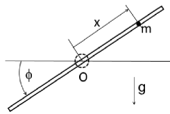
Figure 1. the tube and the ball

A thin tube can rotate freely in the vertical plane about a fixed horizontal axis passing through its centre $O$. A moment of inertia of the tube about this axis is equal to $J$. The mass of the tube is distributed symmetrically such that tube’s centre of mass is placed at the point $O$.

Inside the tube there is a small ball which can slide without friction. The mass of the ball is $m$. The ball can pass by the point $O$ and fall out from the ends of the tube.

The system undergoes the standard gravity field $\boldsymbol{g}$.

It seems to be evident that for typical motion the ball reaches an end of the tube and falls down out the tube. It is surprisingly, at least for the first glance, that this system has very many periodic solutions such that the tube turns around several times during the period.

The sense of generalized coordinates $\phi,x$ is clear from Figure 1.

The Lagrangian of this system is as follows

$$L(x,\phi,\dot{x},\dot{\phi})=\frac{1}{2}\Big{(}mx^{2}+J\Big{)}\dot{\phi}^{2}+\frac{1}{2}m\dot{x}^{2}-mgx\sin\phi.$$ (2.13)

Form theorem 2.1 it follows that for any constant $\omega>0$ system (2.13) has a solution $\phi(t),x(t),\quad t\in\mathbb{R}$ such that

1) $x(t)=-x(-t),\quad\phi(t)=-\phi(-t);$

2) $x(t+\omega)=x(t),\quad\phi(t+\omega)=\phi(t)+2\pi.$

This result shows that for any $\omega>0$ the system has an $\omega-$periodic motion such that the tube turns around once during the period. The length of the tube should be chosen properly.

Our second example is a counterexample. Let us show that the first condition of the theorem 2.1 can not be omitted.

Consider a mass point $m$ that slides on a right circular cylinder of radius $r$. The surface of the cylinder is perfectly smooth. The axis $x$ of the cylinder is parallel to the gravity $\boldsymbol{g}$ and directed upwards.

The Lagrangian of this system is

$$L(x,\varphi,\dot{x},\dot{\varphi})=\frac{m}{2}\Big{(}r^{2}\dot{\varphi}^{2}+\dot{x}^{2}\Big{)}-mgx.$$ (2.14)

All the conditions except the evenness are satisfied but it is clear this system does not have periodic solutions.

3. Proof of Theorem 2.1

In this section we use several standard facts from functional analysis and the Sobolev spaces theory [6], [1].

By $c_{1},c_{2},\ldots$ we denote inessential positive constants.

3.1.

Recall that the Sobolev space $H^{1}_{\mathrm{loc}}(\mathbb{R})$ consists of functions $u(t),t\in\mathbb{R}$ such that $u,\dot{u}\in L^{2}_{\mathrm{loc}}(\mathbb{R})$. The following embedding holds $H^{1}_{\mathrm{loc}}(\mathbb{R})\subset C(\mathbb{R})$.

Recall another standard fact.

Lemma 3.1.

Let $u\in H^{1}_{\mathrm{loc}}(\mathbb{R})$ and $u(0)=0$. Then for any $a>0$ we have

$$\|u\|^{2}_{L^{2}(0,a)}\leq\frac{a^{2}}{2}\|\dot{u}\|^{2}_{L^{2}(0,a)},\quad\|u\|^{2}_{C[0,a]}\leq a\|\dot{u}\|^{2}_{L^{2}(0,a)}.$$

Here and below the notation $\|\dot{u}\|_{L^{2}(0,a)}$ implies that

$$\Big{\|}\dot{u}\Big{|}_{(0,a)}\Big{\|}_{L^{2}(0,a)}$$

the same is concerned to $\|u\|_{C[0,a]}$ etc.

3.2.

Here we collect several spaces which are needed in the sequel.

Definition 4.

By $X$ denote a space of functions $u\in H^{1}_{\mathrm{loc}}(\mathbb{R})$ such that for all $t\in\mathbb{R}$ the following conditions hold

$$u(-t)=-u(t),\quad u(t+\omega)=u(t).$$

By virtue of lemma 3.1, the mapping $u\mapsto\|\dot{u}\|_{L^{2}(0,\omega)}$ determines a norm in $X$. This norm is denoted by $\|u\|$. The norm $\|\cdot\|$ is equivalent to the standard norm of $H^{1}[0,\omega]$. The space $(X,\|\cdot\|)$ is a Banach space. Since the norm $\|\cdot\|$ is generated by an inner product

$$(u,v)_{X}=\int_{0}^{\omega}\dot{u}(t)\dot{v}(t)dt$$

the space $X$ is also a real Hilbert space, particularly this implies that $X$ is a reflexive Banach space.

Definition 5.

Let $\Phi$ stand for the space $\{ct+u(t)\mid c\in\mathbb{R},\quad u\in X\}$.

By the same argument, $(\Phi,\|\cdot\|)$ is a reflexive Banach space. Observe also that $\Phi=\mathbb{R}\oplus X$ and by direct calculation we get

$$\|\psi\|^{2}=\omega c^{2}+\|u\|^{2},\quad\psi(t)=ct+u(t)\in\Phi.$$

Observe that $X\subset\Phi$.

Definition 6.

Let $E$ stand for the space

$$X^{m}\times\Phi^{n}=\{z(t)=(x^{1},\ldots,x^{m},\varphi^{1},\ldots,\varphi^{n})(t)\mid x^{i}\in X,\quad\varphi^{j}\in\Phi\}.$$

The space $E$ is also a real Hilbert space with an inner product defined as follows

$$(z,y)_{E}=\int_{0}^{\omega}\sum_{i=1}^{m+n}\dot{z}^{i}(t)\dot{y}^{i}(t)dt,$$

where $z=(z^{k}),y=(y^{k})\in E,\quad k=1,\ldots,m+n.$

We denote the corresponding norm in $E$ by the same symbol and write

$$\|z\|^{2}=\big{\|}|z|\big{\|}^{2}=\sum_{k=1}^{m+n}\|z^{k}\|^{2}.$$

The space $E$ is also a reflexive Banach space.

Introduce the following set

$$E_{0}=\Big{\{}(x,\varphi)\in E\Big{|}\varphi^{j}=\frac{2\pi\nu_{j}}{\omega}t+u_{j},\quad\forall x\in X,\quad\forall u_{j}\in X,\quad j=1,\ldots,n\Big{\}}.$$

This set is a closed plane of codimension $n$ in $E$.

If $(x,\varphi)\in E_{0}$ then $\varphi(t+\omega)=\varphi(t)+2\pi\nu.$

Definition 7.

Let $Y$ stand for the space

$$\big{\{}u\in L^{2}_{\mathrm{loc}}(\mathbb{R})\mid u(t)=u(-t),\quad u(t+\omega)=u(t)\quad\mbox{almost everywhere in }\mathbb{R}\big{\}}.$$

The space $Y^{m+n}$ is a Hilbert space with respect to the inner product

$$(z,y)_{Y}=\int_{0}^{\omega}\sum_{i=1}^{m+n}z^{i}(t)y^{i}(t)dt,$$

where $z=(z^{k}),y=(y^{k})\in Y^{m+n},\quad k=1,\ldots,m+n.$

3.3.

Fix a positive constant $K_{1}$ and consider a function

$$u:[0,\omega]\to\Sigma,\quad u(t)=(u^{1},\ldots,u^{m+n})(t),\quad u^{i}\in H^{1}[0,\omega]$$ (3.1)

such that the following two conditions hold

$$\int_{0}^{\omega}\frac{dt}{|u(t)-\hat{u}|^{2}}\leq K_{1},\quad\|u\|_{H^{1}[0,\omega]}\leq K_{1}$$ (3.2)

with some constant vector $\hat{u}\in\mathbb{R}^{m+n}$.

Lemma 3.2.

There exists a positive constant $K_{2}$ such that for any function $u$ that satisfies (3.1) and (3.2) one has

$$|u(t)-\hat{u}|\geq K_{2}\sqrt{\sum_{k=1}^{n+m}\|u^{k}-\hat{u}^{k}\|^{2}_{C^{0,1/2}[0,\omega]}},\quad t\in[0,\omega],\quad j=1,\ldots,N.$$

The constant $K_{2}$ depends only on $K_{1}$.

Here $C^{0,1/2}[0,\omega]$ is the Holder space.

Proof of Lemma 3.2. By $c_{1},c_{2},\ldots$ we denote inessential positive constants.

Observe that $H^{1}[0,\omega]\subset C^{0,1/2}[0,\omega]$ and

$$\|\cdot\|_{C^{0,1/2}[0,\omega]}\leq c_{1}\|\cdot\|_{H^{1}[0,\omega]}.$$ (3.3)

Take arbitrary $t^{\prime}\in[0,\omega]$. Fix $j$ and introduce the following notations $v=(v^{1},\ldots,v^{m+n}),$

$$v^{k}=u^{k}-\hat{u}^{k},\quad a=|v(t^{\prime})|,\quad b=\sqrt{\sum_{k=1}^{n+m}\|v^{k}\|^{2}_{C^{0,1/2}[0,\omega]}}.$$

Observe that from conditions of the Lemma and formula (3.3) we get

$$b\leq c_{3}.$$ (3.4)

It follows that

$$|v^{k}(t)-v^{k}(t^{\prime})|\leq\|v^{k}\|_{C^{0,1/2}[0,\omega]}|t-t^{\prime}|^{1/2},\quad t\in[0,\omega]$$

and

$$|v^{k}(t)|\leq|v^{k}(t^{\prime})|+\|v^{k}\|_{C^{0,1/2}[0,\omega]}|t-t^{\prime}|^{1/2}.$$

Consequently, we obtain

$$|v(t)|\leq a+b|t-t^{\prime}|^{1/2}.$$

We then have

$$K_{1}\geq\int_{0}^{\omega}\frac{dt}{|v(t)|^{2}}\geq\int_{0}^{t^{\prime}}\frac{dt}{\big{(}a+b(t^{\prime}-t)^{1/2}\big{)}^{2}}+\int_{t^{\prime}}^{\omega}\frac{dt}{\big{(}a+b(t-t^{\prime})^{1/2}\big{)}^{2}}.$$

The last two integrals are computed easily with the help of the change $\xi=a+b(t^{\prime}-t)^{1/2}$ for the first integral, and $\xi=a+b(t-t^{\prime})^{1/2}$ for the second integral respectively.

Assume for definiteness that $t^{\prime}\in[0,\omega/2]$. Other case is carried out analogously. Then inequality

$$\int_{t^{\prime}}^{\omega}\frac{dt}{\big{(}a+b(t-t^{\prime})^{1/2}\big{)}^{2}}\leq K_{1}$$

and formula (3.4) imply

$$a\geq c_{2}b.$$

The Lemma is proved.

Definition 8.

Let $W$ stand for a set $E_{0}\cap\mathcal{[}\tilde{z}].$

3.4.

Introduce the Action Functional $S:W\to\mathbb{R},$

$$S(z)=\int_{0}^{\omega}L(t,z,\dot{z})dt.$$

Our next goal is to prove that this functional attains its minimum.

By using estimates (2.2), (2.3) we get

$$S(z)\geq\int_{0}^{\omega}\big{(}K|\dot{z}|^{2}-|\dot{z}|(C+M|z|)-A|z|^{2}\big{)}dt.$$

From the Cauchy inequality and Lemma 3.1 it follows that

$$\int_{0}^{\omega}|\dot{z}||z|dt \leq\frac{\omega}{\sqrt{2}}\|z\|^{2},$$

$$\int_{0}^{\omega}|z|^{2}dt \leq\frac{\omega^{2}}{2}\|z\|^{2},$$

$$\int_{0}^{\omega}|\dot{z}|dt \leq\sqrt{\omega}\|z\|.$$

We finally obtain

$$S(z)\geq\Big{(}K-\frac{M\omega}{\sqrt{2}}-\frac{A\omega^{2}}{2}\Big{)}\|z\|^{2}-C\sqrt{\omega}\|z\|.$$ (3.5)

By formula (2.11) the functional $S$ is coercive:

$$S(z)\to\infty$$ (3.6)

as $\|z\|\to\infty.$

Note that the Action Functional which corresponds to system (2.14) is also coercive but, as we see above, property (3.6) by itself does not imply existence results.

3.5.

Let $\{z_{k}\}\subset W$ be a minimizing sequence:

$$S(z_{k})\to\inf_{z\in W}S(z)$$

as $k\to\infty.$

By formula (3.6) the sequence $\{z_{k}\}$ is bounded: $\sup_{k}\|z_{k}\|<\infty.$

Lemma 3.3.

The following estimates hold

$$\inf\{|z_{k}(t)- \sigma^{\prime}|\mid t\in\mathbb{R},\quad\sigma^{\prime}\in\sigma,\quad k\in\mathbb{N}\}$$

$$=\inf\{|z_{k}(t)-\sigma^{\prime}|\mid t\in[0,\omega],\quad\sigma^{\prime}\in\sigma,\quad k\in\mathbb{N}\}>0.$$ (3.7)

Proof of lemma 3.3. The middle equality in formula (3.7) follows from the fact that $z_{k}\in\mathcal{V}_{\nu}$, we will prove inequality.

It is sufficient to check inequality (3.7) for $\sigma^{\prime}\in\sigma\cap\Lambda,$

$$\Lambda=\bigcup_{k\in\mathbb{N}}\{z\in\mathbb{R}^{m+n}\mid|z-z_{k}(t)|\leq 1,\quad t\in[0,\omega]\}.$$

The set $\sigma\cap\Lambda$ is finite.

By formula (2.3) we obtain

$$P\int_{0}^{\omega} \frac{dt}{|z_{k}(t)-\sigma^{\prime}|^{2}}+\Psi_{k}$$

$$\leq c_{7}-\int_{0}^{\omega}V(t,z_{k}(t))dt+\Psi_{k}\leq S(z_{k})+c_{7}.$$ (3.8)

Here

$$\Psi_{k}=\int_{0}^{\omega}a_{i}(t,z_{k}(t))\dot{z}_{k}(t)dt,\quad c_{7}=A\|z_{k}\|^{2}_{L^{2}[0,\omega]}+C_{1}\omega.$$

By formula (2.2) and lemma 3.1 this sequence is bounded:

$$|\Psi_{k}|\leq c_{5}\|z_{k}\|+c_{6}\|z_{k}\|^{2}.$$

So that from formulas (3.8), (2.12) and Lemma 3.2, Lemma 3.3 is proved.

Since the space $E$ is reflexive, this sequence contains a weakly convergent subsequence. Denote this subsequence in the same way: $z_{k}\to z_{*}$ weakly in $E$.

Moreover, the space $H^{1}[0,\omega]$ is compactly embedded in $C[0,\omega]$. Thus extracting a subsequence from the subsequence and keeping the same notation we also have

$$\max_{t\in[0,\omega]}|z_{k}(t)-z_{*}(t)|\to 0,$$ (3.9)

as $k\to\infty$; and

$$\inf\{|z_{*}(t)-\sigma^{\prime}|\mid t\in\mathbb{R},\quad\sigma^{\prime}\in\sigma\}>0.$$

The set $E_{0}$ is convex and strongly closed therefore it is weakly closed: $z_{*}\in E_{0}$. By continuity (3.9) one also gets $z_{*}\in W$ (see Lemma 4.1 in the Appendix).

3.6.

Let us show that $\inf_{z\in W}S(z)=S(z_{*}).$

Lemma 3.4.

Let a sequence $\{u_{k}\}\subset\Phi$ weakly converge to $u\in\Phi$ (or $u_{k},u\in X$ and $u_{k}\to u$ weakly in $X$); and also $\max_{t\in[0,\omega]}|u_{k}(t)-u(t)|\to 0$ as $k\to\infty$.

Then for any $f\in C(\mathbb{R})$ and for any $v\in L^{2}(0,\omega)$ it follows that

$$\int_{0}^{\omega}f(u_{k})\dot{u}_{k}vdt\to\int_{0}^{\omega}f(u)\dot{u}vdt,\quad\mbox{as}\quad k\to\infty.$$

Indeed,

$$\int_{0}^{\omega} f(u_{k})\dot{u}_{k}vdt$$

$$=\int_{0}^{\omega}\big{(}f(u_{k})-f(u)\big{)}\dot{u}_{k}vdt+\int_{0}^{\omega}f(u)\dot{u}_{k}vdt.$$

The function $f$ is uniformly continuous in a compact set

$$\Big{[}\min_{t\in[0,\omega]}\{u(t)\}-c,\max_{t\in[0,\omega]}\{u(t)\}+c\Big{]}$$

with some constant $c>0$. Consequently we obtain

$$\max_{t\in[0,\omega]}|f(u_{k}(t))-f(u(t))|\to 0.$$

Since the sequence $\{u_{k}\}$ is weakly convergent it is bounded:

$$\sup_{k}\|u_{k}\|<\infty$$

particularly, we get

$$\|\dot{u}_{k}\|_{L^{2}(0,\omega)}<\infty.$$

So that as $k\to\infty$

$$\Big{|} \int_{0}^{\omega}\big{(}f(u_{k})-f(u)\big{)}\dot{u}_{k}vdt\Big{|}$$

$$\leq\big{\|}v\big{(}f(u_{k})-f(u)\big{)}\big{\|}_{L^{2}(0,\omega)}\cdot\|\dot{u}_{k}\|_{L^{2}(0,\omega)}\to 0.$$

To finish the proof it remains to observe that a function

$$w\mapsto\int_{0}^{\omega}f(u)\dot{w}vdt$$

belongs to $\Phi^{\prime}$ (or to $X^{\prime}$). Indeed,

$$\Big{|}\int_{0}^{\omega}f(u)\dot{w}vdt\Big{|}\leq\max_{t\in[0,\omega]}|f(u(t))|\cdot\|v\|_{L^{2}(0,\omega)}\|w\|.$$

3.7.

The following lemma is proved similarly.

Lemma 3.5.

Let a sequence $\{u_{k}\}\subset\Phi$ (or $\{u_{k}\}\subset X$) be such that

$$\max_{t\in[0,\omega]}|u_{k}(t)-u(t)|\to 0$$

as $k\to\infty.$

Then for any $f\in C(\mathbb{R})$ and for any $v\in L^{1}(0,\omega)$ it follows that

$$\int_{0}^{\omega}f(u_{k})vdt\to\int_{0}^{\omega}f(u)vdt$$

as $k\to\infty.$

3.8.

Introduce a function $p_{k}(t,\xi)=L(t,z_{k},\dot{z}_{*}+\xi)$. The function $p_{k}$ is a quadratic polynomial of $\xi\in\mathbb{R}^{m+n}$, so that

$$p_{k}(t,\xi)=L(t,z_{k},\dot{z}_{*})+\frac{\partial L}{\partial\dot{z}^{i}}(t,z_{k},\dot{z}_{*})\xi^{i}+\frac{1}{2}\frac{\partial^{2}L}{\partial\dot{z}^{j}\partial\dot{z}^{i}}(t,z_{k},\dot{z}_{*})\xi^{i}\xi^{j}.$$

The last term in this formula is non-negative:

$$\frac{\partial^{2}L}{\partial\dot{z}^{j}\partial\dot{z}^{i}}(t,z_{k},\dot{z}_{*})\xi^{i}\xi^{j}=g_{ij}(t,z_{k})\xi^{i}\xi^{j}\geq 0.$$

We consequently obtain

$$p_{k}(t,\xi)\geq L(t,z_{k},\dot{z}_{*})+\frac{\partial L}{\partial\dot{z}^{i}}(t,z_{k},\dot{z}_{*})\xi^{i}.$$

It follows that

$$S(z_{k}) =\int_{0}^{\omega}p_{k}(t,\dot{z}_{k}-\dot{z}_{*})dt\geq\int_{0}^{\omega}L(t,z_{k},\dot{z}_{*})dt$$

$$+\int_{0}^{\omega}\frac{\partial L}{\partial\dot{z}^{i}}(t,z_{k},\dot{z}_{*})(\dot{z}_{k}^{i}-\dot{z}_{*}^{i})dt.$$ (3.10)

From Lemma 3.4 and Lemma 3.5 it follows that

$$\int_{0}^{\omega}L(t,z_{k},\dot{z}_{*})dt\to\int_{0}^{\omega}L(t,z_{*},\dot{z}_{*})dt\quad\mbox{as}\quad k\to\infty,$$

and

$$\int_{0}^{\omega}\frac{\partial L}{\partial\dot{z}^{i}}(t,z_{k},\dot{z}_{*})(\dot{z}_{k}^{i}-\dot{z}_{*}^{i})dt\to 0\quad\mbox{as}\quad k\to\infty.$$

Passing to the limit as $k\to\infty$ in (3.10) we finally yield

$$\inf_{z\in W}S(z)\geq S(z_{*})\Longrightarrow\inf_{z\in W}S(z)=S(z_{*}).$$

Remark 7.

Basing upon these formulas one can estimate the norm $\|z_{*}\|$. Indeed, take a function $\hat{z}\in W$ then due to formula (3.5) one obtains

$$S(\hat{z})\geq S(z_{*})\geq\Big{(}K-\frac{M\omega}{\sqrt{2}}-\frac{A\omega^{2}}{2}\Big{)}\|z_{*}\|^{2}-C\sqrt{\omega}\|z_{*}\|,$$

here $S(\hat{z})$ is an explicitly calculable number.

3.9.

Now from this point we begin proving the theorem under the assumption that the constraints are odd (2.6).

Thus for any $v\in X^{m+n}$ such that

$$\frac{\partial f_{j}}{\partial z^{k}}(t,z_{*})v^{k}(t)=0$$

it follows that

$$\frac{d}{d\varepsilon}\Big{|}_{\varepsilon=0}S(z_{*}+\varepsilon v)=0.$$

Introduce a linear functional

$$b:X^{m+n}\to\mathbb{R},\quad b(v)=\frac{d}{d\varepsilon}\Big{|}_{\varepsilon=0}S(z_{*}+\varepsilon v),$$

and a linear operator

$$A:X^{m+n}\to X^{l},\quad(Av)_{j}=\frac{\partial f_{j}}{\partial z^{k}}(t,z_{*})v^{k}.$$

It is clear, both these mappings are bounded and

$$\ker A\subset\ker b.$$

Lemma 3.6.

The operator $A$ maps $X^{m+n}$ onto $X^{l}$ that is

$$A(X^{m+n})=X^{l}.$$

Proof. By $\tilde{A}(t)$ denote the matrix

$$\frac{\partial f_{j}}{\partial z^{k}}\big{(}t,z_{*}(t)\big{)}.$$

It is convenient to consider our functions to be defined on the circle $t\in\mathbb{S}=\mathbb{R}/(\omega\mathbb{Z}).$

Fix an element $w\in X^{l}$. Let us cover the circle $\mathbb{S}$ with open intervals $U_{i},\quad i=1,\ldots,N$ such that there exists a set of functions

$$v_{i}\in H^{1}(U_{i}),\quad\tilde{A}(t)v_{i}(t)=w(t),\quad t\in U_{i},\quad i=1,\ldots,N.$$

And let $\psi_{i}$ be a smooth partition of unity subordinated to the covering $\{U_{i}\}$. A function $\tilde{v}(t)=\sum_{i=1}^{N}\psi_{i}(t)v_{i}(t)$ belongs to $H^{1}(\mathbb{S})$ and for each $t$ it follows that $\tilde{A}(t)\tilde{v}(t)=w(t)$. But the function $\tilde{v}$ is not obliged to be odd.

Since $\tilde{A}(-t)=\tilde{A}(t)$ we have

$$\tilde{A}(t)v(t)=w(t),\quad v(t)=\frac{\tilde{v}(t)-\tilde{v}(-t)}{2}\in X^{m+n}.$$

The Lemma is proved.

3.10.

Recall a lemma from functional analysis [8].

Lemma 3.7.

Let $E,H,G$ be Banach spaces and

$$A:E\to H,\quad B:E\to G$$

be bounded linear operators; $\ker A\subseteq\ker B.$

If the operator $A$ is onto then there exists a bounded operator $\Gamma:H\to G$ such that $B=\Gamma A.$

Thus there is a linear function $\Gamma\in(X^{l})^{\prime}$ such that

$$b(v)=\Gamma A(v),\quad v\in X^{m+n}.$$

Or by virtue of the Riesz representation theorem, there exists a set of functions $\{\gamma^{1},\ldots,\gamma^{l}\}\subset X$ such that

$$\frac{d}{d\varepsilon}\Big{|}_{\varepsilon=0}S(z_{*}+\varepsilon v)=\int_{0}^{\omega}\dot{\gamma}^{j}(t)\frac{d}{dt}\Big{(}\frac{\partial f_{j}}{\partial z^{k}}(t,z_{*})v^{k}(t)\Big{)}dt$$

for all $v\in X^{m+n}$.

3.11.

Every element $v\in X^{m+n}$ is presented as follows

$$v(t)=\int_{0}^{t}y(s)ds,$$

where $y\in Y^{m+n}$ is such that

$$\int_{0}^{\omega}y(s)ds=0.$$

Introduce a linear operator $h:Y^{m+n}\to\mathbb{R}^{m+n}$ by the formula

$$h(y)=\int_{0}^{\omega}y(s)ds.$$

Define a linear functional $q:Y^{m+n}\to\mathbb{R}$ by the formula

$$q(y)=(b-\Gamma A)v,\quad v(t)=\int_{0}^{t}y(s)ds.$$

Now all our observations lead to

$$\ker h\subseteq\ker q.$$

Therefore, there exists a linear functional $\lambda:\mathbb{R}^{m+n}\to\mathbb{R}$ such that

$$q=\lambda h$$

Let us rewrite the last formula explicitly. There are real constants $\lambda_{k}$ such that for any $y^{k}\in Y$ one has

$$\int_{0}^{\omega}\Big{(}\frac{\partial L}{\partial\dot{z}^{k}}(t,z_{*},\dot{z}_{*})y^{k}(t)+\frac{\partial L}{\partial z^{k}}(t,z_{*},\dot{z}_{*})\int_{0}^{t}y^{k}(s)ds\Big{)}dt$$

$$=\int_{0}^{\omega}\dot{\gamma}^{j}(t)\frac{\partial f_{j}}{\partial z^{k}}(t,z_{*})y^{k}(t)dt+\int_{0}^{\omega}\dot{\gamma}^{j}(t)\frac{d}{dt}\Big{(}\frac{\partial f_{j}}{\partial z^{k}}(t,z_{*})\Big{)}\int_{0}^{t}y^{k}(s)dsdt$$

$$+\lambda_{k}\int_{0}^{\omega}y^{k}(s)ds.$$

3.12.

By the Fubini theorem we obtain

$$\int_{0}^{\omega}\frac{\partial L}{\partial\dot{z}^{k}}(t,z_{*},\dot{z}_{*})y^{k}(t)dt+\int_{0}^{\omega}y^{k}(s)\int_{s}^{\omega}\frac{\partial L}{\partial z^{k}}(t,z_{*},\dot{z}_{*})dtds$$

$$=\int_{0}^{\omega}\dot{\gamma}^{j}(t)\frac{\partial f_{j}}{\partial z^{k}}(t,z_{*})y^{k}(t)dt+\int_{0}^{\omega}y^{k}(s)\int_{s}^{\omega}\dot{\gamma}^{j}(t)\frac{d}{dt}\Big{(}\frac{\partial f_{j}}{\partial z^{k}}(t,z_{*})\Big{)}dtds$$

$$+\lambda_{k}\int_{0}^{\omega}y^{k}(s)ds.$$ (3.11)

In this formula the functions

$$\frac{\partial L}{\partial\dot{z}^{k}}(t,z_{*},\dot{z}_{*}),\quad\dot{\gamma}^{j}(t)\frac{\partial f_{j}}{\partial z^{k}}(t,z_{*})$$

are even and $\omega$-periodic functions of $t$.

The functions

$$\dot{\gamma}^{j}(t)\frac{d}{dt}\Big{(}\frac{\partial f_{j}}{\partial z^{k}}(t,z_{*})\Big{)},\quad\frac{\partial L}{\partial z^{k}}(t,z_{*},\dot{z}_{*})$$

are odd and $\omega$-periodic.

Employ the following trivial observation.

Proposition 2.

If $w\in L^{1}_{\mathrm{loc}}(\mathbb{R})$ is an $\omega-$periodic and odd function then for any constant $a\in\mathbb{R}$ a function

$$t\mapsto\int_{a}^{t}w(s)ds$$

is also $\omega-$periodic.

So that the functions

$$\int_{s}^{\omega}\dot{\gamma}^{j}(t)\frac{d}{dt}\Big{(}\frac{\partial f_{j}}{\partial z^{k}}(t,z_{*})\Big{)}ds,\quad\int_{s}^{\omega}\frac{\partial L}{\partial z^{k}}(t,z_{*},\dot{z}_{*})ds$$

are even and $\omega$-periodic in $s$.

Therefore, equation (3.11) is rewritten as $(y,\eta)_{Y}=0$ for any $y=(y^{1},\ldots y^{m+n})\in Y^{m+n}$ and $\eta=(\eta_{1},\ldots,\eta_{m+n})$ stands for

$$\eta_{k} =\frac{\partial L}{\partial\dot{z}^{k}}(t,z_{*},\dot{z}_{*})+\int_{t}^{\omega}\frac{\partial L}{\partial z^{k}}(s,z_{*},\dot{z}_{*})ds$$

$$-\dot{\gamma}^{j}(t)\frac{\partial f_{j}}{\partial z^{k}}(t,z_{*})-\int_{t}^{\omega}\dot{\gamma}^{j}(s)\frac{d}{ds}\Big{(}\frac{\partial f_{j}}{\partial z^{k}}(s,z_{*})\Big{)}ds-\lambda_{k}\in Y.$$

Consequently we obtain the following system

$$\frac{\partial L}{\partial\dot{z}^{k}}(t,z_{*},\dot{z}_{*})+\int_{t}^{\omega}\frac{\partial L}{\partial z^{k}}(s,z_{*},\dot{z}_{*})ds$$

$$=\dot{\gamma}^{j}(t)\frac{\partial f_{j}}{\partial z^{k}}(t,z_{*})+\int_{t}^{\omega}\dot{\gamma}^{j}(s)\frac{d}{ds}\Big{(}\frac{\partial f_{j}}{\partial z^{k}}(s,z_{*})\Big{)}ds+\lambda_{k}.$$ (3.12)

here $k=1,\ldots,m+n.$

If we formally differentiate both sides of equations (3.12) in $t$ then we obtain the Lagrange equations (2.9) with $\alpha^{j}=\ddot{\gamma}^{j}$.

Equations (3.12) hold for almost all $t\in(0,\omega)$ but all the functions contained in (3.12) are defined for all $t\in\mathbb{R}$.

The functions

$$\int_{t}^{\omega}\dot{\gamma}^{j}(s)\frac{d}{ds}\Big{(}\frac{\partial f_{j}}{\partial z^{k}}(s,z_{*})\Big{)}ds,\quad\int_{t}^{\omega}\frac{\partial L}{\partial z^{k}}(s,z_{*},\dot{z}_{*})ds$$

are $\omega-$periodic by Proposition 2. Equation (3.12) holds for almost all $t\in\mathbb{R}$.

3.13.

Let $g^{ij}$ stand for the components of the matrix inverse to $(g_{ij}):\quad g^{ij}g_{ik}=\delta_{k}^{j}$. Present equation (3.12) in the form

$$\dot{z}^{j}_{*}(t) =g^{kj}(t,z_{*}(t))$$

$$\cdot\Big{(}\lambda_{k}+\dot{\gamma}^{i}(t)\frac{\partial f_{i}}{\partial z^{k}}(t,z_{*}(t))+\int_{t}^{\omega}\dot{\gamma}^{i}(s)\frac{d}{ds}\Big{(}\frac{\partial f_{i}}{\partial z^{k}}(s,z_{*}(s))\Big{)}ds$$

$$-\int_{t}^{\omega}\frac{\partial L}{\partial z^{k}}(s,z_{*}(s),\dot{z}_{*}(s))ds-a_{k}(t,z_{*}(t))\Big{)}.$$ (3.13)

Together with equation (3.13) consider equations

$$\frac{\partial f_{j}}{\partial t}(t,z_{*}(t))+\frac{\partial f_{j}}{\partial z^{k}}(t,z_{*}(t))\dot{z}^{k}_{*}(t)=0.$$ (3.14)

These equations follow from (2.4).

Recall that by the Sobolev embedding theorem, $z_{*}\in X\subset C(\mathbb{R}).$

Due to (2.5) we have

$$\det B(t,z_{*})\neq 0,\quad B(t,z_{*})=\Big{(}g^{kj}(t,z_{*})\frac{\partial f_{i}}{\partial z^{k}}(t,z_{*})\frac{\partial f_{l}}{\partial z^{j}}(t,z_{*})\Big{)}$$

for all $t$. Substituting $\dot{z}_{*}$ from (3.13) to (3.14) we can express $\dot{\gamma}^{j}$ and see $\dot{\gamma}^{j}\in C(\mathbb{R})$. Thus from (3.13) it follows that $\dot{z}_{*}\in C(\mathbb{R}).$

Applying this argument again we obtain $\ddot{\gamma}^{j},\ddot{z}_{*}\in C(\mathbb{R}).$

This proves the theorem for the case of odd constraints.

3.14.

Let us discuss the proof of the theorem under the assumption that the constraints are even (2.7).

Definition 9.

By $Z$ denote a space of functions $u\in H^{1}_{\mathrm{loc}}(\mathbb{R})$ such that for all $t\in\mathbb{R}$ the following conditions hold

$$u(-t)=u(t),\quad u(t+\omega)=u(t).$$

The space $Z^{l}$ is a real Hilbert space with respect to an inner product

$$(u,v)_{Z}=\sum_{i=1}^{l}\int_{0}^{\omega}\big{(}u_{i}(t)v_{i}(t)+\dot{u}_{i}(t)\dot{v}_{i}(t)\big{)}dt.$$

This is the standard inner product in $H^{1}[0,\omega]$.

So what is changed now? The operator $A$ takes the space $X^{m+n}$ onto the space $Z^{l}$. The proof of this fact is the same as in Lemma 3.6.

By the Riesz representation theorem, there exists a set of functions $\{\gamma^{1},\ldots,\gamma^{l}\}\subset Z$ such that

$$b(v) =\int_{0}^{\omega}\dot{\gamma}^{j}(t)\frac{d}{dt}\Big{(}\frac{\partial f_{j}}{\partial z^{k}}(t,z_{*})v^{k}(t)\Big{)}dt$$

$$+\int_{0}^{\omega}\gamma^{j}(t)\frac{\partial f_{j}}{\partial z^{k}}(t,z_{*})v^{k}(t)dt$$

for all

$$v=\int_{0}^{t}y(s)ds,\quad y\in Y^{m+n},\quad\int_{0}^{\omega}y(s)ds=0.$$

So that equation (3.12) is replaced with the following one

$$\frac{\partial L}{\partial\dot{z}^{k}}(t,z_{*},\dot{z}_{*})+\int_{t}^{\omega}\frac{\partial L}{\partial z^{k}}(s,z_{*},\dot{z}_{*})ds$$

$$=\dot{\gamma}^{j}(t)\frac{\partial f_{j}}{\partial z^{k}}(t,z_{*})+\int_{t}^{\omega}\dot{\gamma}^{j}(s)\frac{d}{ds}\Big{(}\frac{\partial f_{j}}{\partial z^{k}}(s,z_{*})\Big{)}ds$$

$$+\int_{t}^{\omega}\gamma^{j}(s)\frac{\partial f_{j}}{\partial z^{k}}(s,z_{*})ds+\lambda_{k}.$$

Here $k=1,\ldots,m+n.$ By the same argument the functions

$$\int_{t}^{\omega}\gamma^{j}(s)\frac{\partial f_{j}}{\partial z^{k}}(s,z_{*})ds,\quad\int_{t}^{\omega}\dot{\gamma}^{j}(s)\frac{d}{ds}\Big{(}\frac{\partial f_{j}}{\partial z^{k}}(s,z_{*})\Big{)}ds$$

are $\omega-$periodic and one can put $\alpha^{j}=\ddot{\gamma}^{j}-\gamma^{j}.$

Other argument is the same as above. The theorem is proved.

4. Appendix

Lemma 4.1.

Fix a positive constant $\delta$.

Let $z_{1},z_{2}$ be functions from $\mathcal{V}_{p}$ such that

$$\inf\{|z_{i}(t)-\sigma^{\prime}|\mid t\in[0,\omega],\quad\sigma^{\prime}\in\sigma,\quad i=1,2\}\geq\delta.$$

There exists a positive number $\varepsilon>0$ such that if

$$\max_{t\in[0,\omega]}|z_{1}(t)-z_{2}(t)|<\varepsilon$$

then these functions are homotopic.

Proof of lemma 4.1. Our argument is quite standard. So we present a sketch of the proof.

It is convenient to consider $z_{1},z_{2}$ as functions with values in $\mathcal{C}$ (see Remark 1). In the same sense $F(t)$ is a submanifold in $\mathcal{C}$ and the functions $z_{1},z_{2}$ define a pair of closed curves in $\mathcal{C}$.

Choose a Riemann metric in $\mathcal{C}$, for example as follows

$$d\tau^{2}=\sum_{k=1}^{m+n}(dz^{k})^{2}.$$

This metric inducts a metric in $F(t)$.

Under the conditions of the Lemma any two points $z_{1}(t),z_{2}(t)\in F(t)$ are connected in $F(t)$ with a unique shortest piece of geodesic $\chi(\xi,t),\quad\xi\in[0,\tilde{\xi}(t)]$ such that

$$\chi(0,t)=z_{1}(t),\quad\chi(\tilde{\xi}(t),t)=z_{2}(t).$$

Here $\xi$ is the arc-length parameter.

Define the homotopy as follows $z(s,t)=\chi(s\tilde{\xi}(t),t),\quad s\in[0,1]$.

The Lemma is proved.

Acknowledgments

The author wishes to thank Professor E. I. Kugushev for useful discussions.

References

- [1] R. A. Adams J.J.F. Fournier: Sobolev Spaces, Elsevier, 2nd Edn. 2003.
- [2] V. Arnold: Mathematical Methods of Classical Mechanics. Springer-Verlag New York, 1989.
- [3] A. Capozzi, D. Fortunato, A. Salvatore: Periodic Solutions of Lagrangian Systems with Bounded Potential, Journal of Mathematical Analysis and Applications, Vol.124, p.482-494 (1987)
- [4] I. Gerasimov: Euler’s Problem of Two Fixed Centers. Moscow State University, 2007. (In Russian)
- [5] Govind S. Krishnaswami and Himalaya Senapati: Curvature and geodesic instabilities in a geometrical approach to the planar three-body problem, J. Math. Phys. 57, 102901 (2016).
- [6] R. Edwards: Functional Analysis. New York, 1965.
- [7] I. Ekeland, R. Témam, Convex Analysis and Variational Problems, Society for Industrial and Applied Mathematics (SIAM), Philadelphia, PA, 1999.
- [8] A. Kolmogorov, S. Fomin: Elements of the Theory of Functions and Functional Analysis. Ukraine, 1999.
- [9] R. P. Martinez-y-Romero, 1 H. N. Nunez-Yepez, 2 and A. L. Salas-Brito: The two dimensional motion of a particle in an inverse square potential: Classical and quantum aspects. Journal of Mathematical PHysics, 54, 053509 (2013)
- [10] J. Mawhin, M. Willem, Critical Point Theory and Hamiltonian Systems, Springer-Verlag, New York, 1989.
- [11] M. Struwe, Variational Methods, Springer-Verlag, Berlin, 2008.