An Arbitrary-Order Discontinuous Galerkin Method with One Unknown Per Element

Abstract.

We propose an arbitrary-order discontinuous Galerkin method for second-order elliptic problem on general polygonal mesh with only one degree of freedom per element. This is achieved by locally solving a discrete least-squares over a neighboring element patch. Under a geometrical condition on the element patch, we prove an optimal a priori error estimates for the energy norm and for the L² norm. The accuracy and the efficiency of the method up to order six on several polygonal meshes are illustrated by a set of benchmark problems.

Keyword: least-squares reconstruction, discontinuous Galerkin method, elliptic problem

MSC2010: 49N45; 65N21

1. Introduction

The discontinuous Galerkin method (DG) [37, 17] is by now a very standard numerical method to simulate a wide variety of partial differential equations of scientific or engineer interest. Recently there are quite a few work concerning the discontinuous Galerkin method on general polytopic (polygonal or polyhedral) meshes [26, 19, 2, 30, 14, 44, 12, 13]. Unlike the finite element method [39], the full discontinuity across the element interfaces of the trial and test function spaces of DG method lends itself naturally to the polytopic meshes, which does provide more flexibility in implementation, in particular for domain with microstructures or problems with certain physical constraints. Such meshes may ease the triangulation of complex domains or domains with microstructures. On the other hand, compared to the classical conforming finite element method, the DG method is computationally expensive over a particular computational mesh and approximation order, which is due to the fact that the rapid increasing of the local degrees of freedom. Moreover, for certain problems, such as fluid solid interaction problems or a heat diffusion problem that is coupled or is embed into a compressible fluid problem, there is no enough information to support a large number of local degrees of freedom. Though this problem is partially solved by the agglomeration-based physical frame DG method [7, 6] and the hybrid DG method [16], it is desirable to develop a DG method with less local degrees of freedom while retaining high accuracy.

A common trait is to employ patch reconstruction to achieve high accuracy. To the best of the authors’ knowledge, such reconstruction idea can be traced back to the endeavors on developing three node plate bending elements and simple shell elements in the early 1970s; see, for example [34, 25, 36, 35]. Similar ideas may also be found in WENO [41] and finite volume method for hyperbolic conservation laws [5].

This motivates us to use patches of a piecewise constant function to reconstruct a piecewise high order polynomial on each element, which is achieved by solving a discrete least-squares approximation problem over element patch. Such approach has been used in [29] to reconstruct piecewise effective tensor field from scattered data for the multiscale partial differential equations. This new space is a sub-space of the commonly used finite element space corresponding to DG methods. This new finite element space may be combined with any other DG formulations to numerically solve even more general elliptic problems such as plate bending problem [28], Stokes flow problems, and eigenvalue problems, just name a few. As a starting point, we employ the Interior Penalty discontinuous Galerkin (IPDG) method [3] with this reconstructed finite element space to solve Poisson problem. Under a mild condition on the geometry of the element patch, we proved that this reconstructed finite element space admits optimal approximation properties in certain broken Sobolev norms, by which we proved the optimal error estimates in the DG-energy norm and in the L² norm of the proposed method.

Our method possesses several attractive features. First, arbitrary order accuracy may be achieved with increasing the order of the reconstruction, while there is only one degree of freedom per element, by contrast to the standard DG method, which requires at least three unknowns on each element. From this aspect of view, the proposed method has a flavor of finite volume method. Second, the method can be used on any shape of elements, which may be triangles, quadrilaterals, polygons in two dimension, or tetrahedron, prism, pyramid, hexahedron in three dimension. In particular, the method may be used on the hybrid mesh, which is nowadays quite common in simulations because it can handle the complicated domain or even reduce the total number of unknowns [45]. Third, the reconstruction procedure of the proposed method is stable with respect to the small perturbation of the data, which is of practical interesting due to the measurement error. Our results for the reconstruction procedure is of independent interest for the discrete least-squares [38].

A closely related approach is a special DG method proposed in [27]. The authors introduced a family of continuous linear finite elements for the Kirhhoff-Love plate model. A continuous linear interpolation of the deflection field is employed to reconstruct a discontinuous quadratic deflection field by solving a local least-squares problem over element patch. It is worth mentioning that one of their reconstruction method is the same with the second order constrained reconstruction in [29]. Moreover, this method only applies to structured mesh. Another closely related method is the cell-centered Galerkin method presented in [21]. The authors developed an arbitrary-order discretization method of diffusion problems on general polyhedral mesh. The cornerstone of this method is the locally reconstructed discrete gradient operator and a stabilized term, while our method is the locally reconstructed finite element space. This method has also been successfully extended to mixed form [20] recently.

The rest of the paper is organized as follows. In § 2, we describe the reconstruction finite element space and prove its approximation properties and the stability properties of the reconstruction procedure. In § 3, we present the interior penalty discontinued Galerkin method for Poisson problem with the reconstructed approximation space and prove a priori error estimate, and in § 4, numerical results for second order elliptic problems in two dimension are presented. Finally, in § 5, we summarize the work and draw some conclusions.

Throughout this paper, we shall use standard notations for Sobolev spaces, norms and seminorms, cf. [1]; see, for example, $\|u\|_{H^{1}(D)}{:}=\|\,u\,\|_{L^{2}(D)}+\|\,\nabla u\,\|_{L^{2}(D)}$ for any bounded domain $D$. We use $C$ as a generic constant independent of the mesh size, which may change from line to line. We mainly focus on two dimensional problem though most results are valid in three dimension.

2. Approximation Space

Let $\Omega$ be a polygonal domain in $\mathbb{R}^{2}$. The mesh $\mathcal{T}_{h}$ is a triangulation of $\Omega$ with polygons $K$, which may not be convex. Here $h{:}=\max_{K\in\mathcal{T}_{h}}h_{K}$ with $h_{K}$ the diameter of $K$. We denote $\left\lvert K\right\rvert$ the area of $K$. Let $\mathbb{P}_{n}(D)$ be a set of polynomial in two variables with total degree at most $n$ confined to domain $D$, where $D$ may be an element $K$ or an agglomeration of the elements belong to $\mathcal{T}_{h}$. We assume that the mesh $\mathcal{T}_{h}$ satisfies the following shape regularity conditions, which were introduced originally in [10] to study the convergence of mimetic finite difference. Detailed discussion on such conditions can be found in [8, §1.6].

There exist

1. an integer number $N$ independent of $h$;

2. a real positive number $\sigma$ independent of $h$;

3. a compatible sub-decomposition $\widetilde{\mathcal{T}_{h}}$

such that

1. any element $K$ admits a sub-decomposition $\widetilde{\mathcal{T}_{h}}|_{K}$ that consists of at most $N$ triangles $T$.

2. Any $T\in\widetilde{\mathcal{T}_{h}}$ is shape-regular in the sense of Ciarlet-Raviart [15]: there exists $\sigma$ such that $h_{T}/\rho_{T}\leq\sigma$, where $\rho_{T}$ is the radius of the largest ball inscribed in $T$.

Assumptions A1 and A2 impose quite weak constraints on the triangulation, which may contain elements with quite general shapes, for example, non-convex or degenerate elements are allowed.

The above shape regularity assumptions lead to some useful consequences, which will be extensively used in the later analysis.

1. For any $T\in\widetilde{\mathcal{T}_{h}}$, there exists $\rho_{1}\geq 1$ that depends on $N$ and $\sigma$ such that $h_{K}/h_{T}\leq\rho_{1}$.

2. [Agmon inequality] There exists $C$ that depends on $N$ and $\sigma$, but independent of $h_{K}$ such that

   (2.1) $$\|\,v\,\|_{L^{2}(\partial K)}^{2}\leq C\left(h_{K}^{-1}\|\,v\,\|_{L^{2}(K)}^{2}+h_{K}\|\,\nabla v\,\|_{L^{2}(K)}^{2}\right)\qquad\text{for all\quad}v\in H^{1}(K).$$

3. [Approximation property] There exists $C$ that depends on $N,r$ and $\sigma$, but independent of $h_{K}$ such that for any $v\in H^{r+1}(K)$, there exists an approximation polynomial $\widetilde{v}\in\mathbb{P}_{r}(K)$ such that

   (2.2) $$\|\,v-\widetilde{v}\,\|_{L^{2}(K)}+h_{K}\|\,\nabla(v-\widetilde{v})\,\|_{L^{2}(K)}\leq Ch_{K}^{r+1}\left\lvert\,v\,\right\rvert_{H^{r+1}(K)}.$$

4. [Inverse inequality] For any $v\in\mathbb{P}_{r}(K)$, there exists a constant $C$ that depends only on $N,r,\sigma$ and $\rho_{1}$ such that

   (2.3) $$\|\,\nabla v\,\|_{L^{2}(K)}\leq Ch_{K}^{-1}\|\,v\,\|_{L^{2}(K)}.$$

Note that we have not list all the mesh conditions in [10] and [8, §1.6], while the above two assumptions A1 and A2 suffice for our purpose. The Agmon inequality M2 and the Approximation property M3 have been proved in [8, §1.6.3]. As to M3, one may take the approximation polynomial $\widetilde{v}$ as the averaged Taylor polynomial of order $r+1$ [9]. The inverse inequality M4 can be proved as follows. For any $v\in\mathbb{P}_{r}(K)$, the restriction $v|_{T}\in\mathbb{P}_{r}(T)$, using the following standard inverse inequality on triangle $T$ [15], we have

$$\|\,\nabla v\,\|_{L^{2}(T)}\leq C_{\text{inv}}h_{T}^{-1}\|\,v\,\|_{L^{2}(T)}.$$

where $C_{\text{inv}}$ depends on $\sigma$ and $r$ while is independent of $h_{T}$. Summing up all $T\in\widetilde{T}_{h}|_{K}$, and using M1, we obtain

$$\|\,\nabla v\,\|_{L^{2}(K)}^{2} =\sum_{T\subset\widetilde{\mathcal{T}}_{h}|_{K}}\|\,\nabla v\,\|_{L^{2}(T)}^{2}\leq C_{\text{inv}}^{2}\rho_{1}^{2}h_{K}^{-2}\sum_{T\subset\widetilde{\mathcal{T}}_{h}|_{K}}\|\,v\,\|_{L^{2}(T)}^{2}$$

$$=C_{\text{inv}}^{2}\rho_{1}^{2}h_{K}^{-2}\|\,v\,\|_{L^{2}(K)}^{2}.$$

This gives (2.3) with $C=C_{\text{inv}}\rho_{1}$.

A combination of (2.1) and (2.3) yields the discrete trace inequality: for any $v\in\mathbb{P}_{r}(K)$,

(2.4) $$\|\,v\,\|_{L^{2}(\partial K)}\leq C\left(1+C_{\text{inv}}\rho_{1}\right)h_{K}^{-1/2}\|\,v\,\|_{L^{2}(K)}.$$

Remark 2.1.

The above four inequalities (2.1), (2.2), (2.3) and (2.4) are the foundation to derive the error estimate for the IPDG method [3], which are also valid over the polygonal meshes satisfying different shape regular conditions; see, for example [19, §1.4] and [32]).

2.1. Reconstruction operator

Given the triangulation $\mathcal{T}_{h}$, we define the reconstruction operator in a piecewise manner as follows. For each element $K\in\mathcal{T}_{h}$, we firstly assign a sampling node $x_{K}\in K$ that is preferably in the interior of the element $K$, and construct an element patch $S(K)$. The element patch $S(K)$ usually contains $K$ and some elements around $K$. There are many different ways to find the sampling nodes and construct the element patch. For example, we may let the barycenter of the element $K$ as the sampling node, while it can be more flexible due to the stability property of the least-squares reconstruction; cf. Lemma 2.2. The element patch may be built up in the following two ways. The first way is that we initialize $S(K)$ as $K$, and add all the Moore neighbors (elements with nonempty intersection with the closure of $K$) [40] into $S(K)$ recursively until sufficiently large number of elements are collected into the element patch. Such kind of construction has been used in [29] to reconstruct effective tensor field from scattered data. The second way is the same with the first one except that we use the Von Neumann neighbor (adjacent edge-neighboring elements) [40] instead of Moore neighbor. An example for such $S(K)$ is shown in Figure 2.1. We denote by $t$ the recursion depth for the element patch $S(K)$.

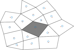
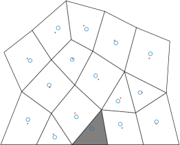
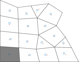
Figure 2.1. The element patches $S(K)$ in the interior of the domain (left), along the boundary of the domain (middle) and at the corner of the domain (right), together with randomly perturbed sampling points for Example 3 in § 4. Here the element $K$ is marked in black and the sampling nodes in $\mathcal{I}(K)$ are the barycenters of the elements, which are marked in dots, and the perturbed sampling nodes in $\widetilde{\mathcal{I}}(K)$ are marked as small circles.

We denote $\mathcal{I}(K)$ the set of the sampling nodes belonging to $S(K)$ with $\#\mathcal{I}(K)$ its cardinality, and let $\#S(K)$ be the number of elements belonging to $S(K)$. These two numbers are equal. We define $d_{K}{:}=\text{diam}\;S(K)$ and $d=\max_{K\in\mathcal{T}_{h}}d_{K}$. Moreover, we assume that $S(K)$ satisfies the following geometrical assumption.

Assumption A  For every $K\in\mathcal{T}_{h}$, there exist constants $R$ and $r$ that are independent of $K$ such that $B_{r}\subset S(K)\subset B_{R}$ with $R\geq 2r$, and $S(K)$ is star-shaped with respect to $B_{r}$, where $B_{\rho}$ is a disk with radius $\rho$.

As a direct consequence of the above assumption, we have the following characterization of $S(K)$.

Lemma 2.1.

If Assumption A is valid, then for all element $K\in\mathcal{T}_{h}$, the element patch $S(K)$ satisfies an interior cone condition, and there exists a uniform bound $\gamma$ for the chunkiness parameter of $S(K)$.

Proof.

By [33, Proposition 2.1], if Assumption A holds true, then the element patch $S(K)$ satisfies an interior cone condition with radius $r$ and angel $\theta=2\arcsin\dfrac{r}{2R}$.

By definition [9, Definition 4.2.16], the chunkiness parameter $\gamma_{K}$ is defined as the ratio between the diameter of $S(K)$ and the radius of the largest ball to which $S(K)$ is star-shaped. This leads to the following bound

$$\gamma_{K}{:}=\dfrac{d_{K}}{r}\leq\dfrac{2R}{r}.$$

Let $\gamma{:}=2R/r$, we obtain a uniform bound on the chunkiness parameter for all $K\in\mathcal{T}_{h}$. ∎

Let $U_{h}$ be the piecewise constant space associated with $\mathcal{T}_{h}$, i.e.,

$$U_{h}{:}=\{\,v\in L^{2}(\Omega)\,\mid\,v|_{K}\in\mathbb{P}_{0}(K)\}.$$

For any $v\in U_{h}$ and for any $K\in\mathcal{T}_{h}$, we reconstruct a high order polynomial $\mathcal{R}_{K}v$ of degree $m$ by solving the following discrete least-squares.

(2.5) $$\mathcal{R}_{K}v=\operatorname{argmin}_{p\in\mathbb{P}_{m}(S(K))}\sum_{x\in\mathcal{I}(K)}\left\lvert v(x)-p(x)\right\rvert^{2}.$$

A global reconstruction operator $\mathcal{R}$ is defined by $\mathcal{R}|_{K}=\mathcal{R}_{K}$. Given $\mathcal{R}$, we embed $U_{h}$ into a discontinuous finite element space with piecewise polynomials of order $m$, and denote $V_{h}=\mathcal{R}U_{h}$.

In what follows, we make the following assumption on the sampling node set $\mathcal{I}(K)$.

Assumption B  For any $K\in\mathcal{T}_{h}$ and $p\in\mathbb{P}_{m}(S(K))$,

(2.6) $$p|_{\mathcal{I}(K)}=0\quad\text{implies\quad}p|_{S(K)}\equiv 0.$$

This assumption implies the uniqueness, and equally the existence of the discrete least-squares (2.5). Assumption B requires that $\#\mathcal{I}(K)$ cannot be too small, which is at least $(m+2)(m+1)/2$ to guarantee the unisolvability of the discrete least-squares. A quantitative version of this assumption is

$$\Lambda(m,\mathcal{I}(K))<\infty$$

with

(2.7) $$\Lambda(m,\mathcal{I}(K)){:}=\max_{p\in\mathbb{P}_{m}(S(K))}\dfrac{\|\,p\,\|_{L^{\infty}(S(K))}}{\|\,p|_{\mathcal{I}(K)}\,\|_{\ell_{\infty}}}.$$

The reconstruction procedure is robust with respect to the small perturbation of the sampling nodes due to the following stability result. In particular, $\Lambda(m,\mathcal{I}(K))$ remains bounded with respect to small perturbation. This problem is of practical interest because both the sampled values and the positions of the sampling nodes are affected by the measurable errors.

Lemma 2.2.

Let $S(K)$ be the element patch defined above and $g\in C^{1}(S(K))$. If we assume that

1. There exists $\alpha>0$ such that

   (2.8) $$\|\,g\,\|_{L^{\infty}(S(K))}\leq\alpha\|\,g|_{\mathcal{I}(K)}\,\|_{\ell_{\infty}}.$$

2. $S(K)$ admits a Markov-type inequality in the sense that there exists $\beta>0$ such that

   (2.9) $$\|\,\nabla g\,\|_{L^{\infty}(S(K))}\leq\beta\|\,g\,\|_{L^{\infty}(S(K))}.$$

Then for any $\delta\in(0,1)$, there exists $\varepsilon=\delta/(\alpha\beta)$ such that for any sampling node set $\widetilde{\mathcal{I}}(K)$ that is a perturbation of $\mathcal{I}(K)$ in the sense that $\widetilde{\mathcal{I}}(K)\subset\mathcal{I}(K)+B(0,\varepsilon)$ with $B$ centers at $0$ with radius $\varepsilon$, the following stability estimate is valid:

(2.10) $$\|\,g\,\|_{L^{\infty}(S(K))}\leq\dfrac{\alpha}{1-\delta}\|\,g|_{\widetilde{\mathcal{I}}(K)}\,\|_{\ell_{\infty}}.$$

This stability estimate for the reconstruction procedure depends on the assumptions (2.8) and (2.9). The validity of these two assumptions hinges on certain geometrical condition on the element patch. For example, if the element patch $S(K)$ is convex, then by [29, Lemma 3.5], the first assumption (2.8) is valid with $\alpha=2$, and the second assumption (2.9) is valid with $\beta=4m^{2}/w(K)$ due to the Markov inequality of Wilhelmsen [43] for the convex domain, where $w(K)$ is the width of the convex set $S(K)$. A more general assumption for the validity of these two assumptions may be found in Remark 2.3.

Proof.

Let $x^{\ast}\in\mathcal{I}(K)$ satisfy $\left\lvert g(x^{\ast})\right\rvert=\|\,g|_{\mathcal{I}(K)}\,\|_{\ell_{\infty}}$. There exists $\widetilde{x}\in\widetilde{\mathcal{I}}(K)$ such that $\left\lvert\widetilde{x}-x^{\ast}\right\rvert\leq\varepsilon$. By Taylor’s expansion,

$$\left\lvert g(x^{\ast})\right\rvert \leq\left\lvert g(\widetilde{x})\right\rvert+\varepsilon\max_{x\in S(K)}\left\lvert\nabla g(x)\right\rvert$$

$$\leq\|\,g|_{\widetilde{\mathcal{I}}(K)}\,\|_{\ell_{\infty}}+\varepsilon\beta\|\,g\,\|_{L^{\infty}(S(K))},$$

where we have used the Markov’s inequality (2.9). Therefore, we obtain

$$\|\,g\,\|_{L^{\infty}(S(K))} \leq\alpha\|\,g|_{\mathcal{I}(K)}\,\|_{\ell_{\infty}}=\alpha\left\lvert g(x^{\ast})\right\rvert$$

$$\leq\alpha\|\,g|_{\widetilde{\mathcal{I}}(K)}\,\|_{\ell_{\infty}}+\varepsilon\alpha\beta\|\,g\,\|_{L^{\infty}(S(K))}$$

$$=\alpha\|\,g|_{\widetilde{\mathcal{I}}(K)}\,\|_{\ell_{\infty}}+\delta\|\,g\,\|_{L^{\infty}(S(K))},$$

which immediately implies the stability estimate (2.10). ∎

The following properties of the reconstruction operator $\mathcal{R}_{K}$ is proved in [29, Theorem 3.3], which is of vital importance to our error estimate.

Lemma 2.3.

If Assumption B holds, then there exists a unique solution of (2.5) for any $K\in\mathcal{T}_{h}$. The unique solution is denoted by $\mathcal{R}_{K}v$.

Moreover $\mathcal{R}_{K}$ satisfies

(2.11) $$\mathcal{R}_{K}g=g\quad\text{for all\quad}g\in\mathbb{P}_{m}(S(K)).$$

The stability property holds true for any $K\in\mathcal{T}_{h}$ and $g\in C^{0}(S(K))$ as

(2.12) $$\|\,\mathcal{R}_{K}g\,\|_{L^{\infty}(K)}\leq\Lambda(m,\mathcal{I}(K))\sqrt{\#\mathcal{I}(K)}\|\,g|_{\mathcal{I}(K)}\,\|_{\ell_{\infty}},$$

and the quasi-optimal approximation property is valid in the sense that

(2.13) $$\|\,g-\mathcal{R}_{K}g\,\|_{L^{\infty}(K)}\leq\Lambda_{m}\inf_{p\in\mathbb{P}_{m}(S(K))}\|\,g-p\,\|_{L^{\infty}(S(K))},$$

where $\Lambda_{m}{:}=\max_{K\in\mathcal{T}_{h}}\{1+\Lambda(m,\mathcal{I}(K))\sqrt{\#\mathcal{I}(K)}\}$.

By the above lemma, we conclude that the reconstruction $\mathcal{R}_{K}g$ is a nearly optimal uniform approximation polynomial to $g$ provided that $\Lambda(m,\mathcal{T}(K))\sqrt{\#\mathcal{I}(K)}$ can be bounded. As a direct consequence of this property, we shall prove below that such nearly optimal approximation property of the reconstruction is also valid with respect to the broken H¹-norms.

Lemma 2.4.

If Assumption B holds, then there exists $C$ that depends on $N,\sigma$ and $\gamma$ such that

(2.14) $$\|\,g-\mathcal{R}_{K}g\,\|_{L^{2}(K)} \leq C\Lambda_{m}h_{K}d_{K}^{m}\left\lvert\,g\,\right\rvert_{H^{m+1}(S(K))}.$$

(2.15) $$\|\,\nabla(g-\mathcal{R}_{K}g)\,\|_{L^{2}(K)} \leq C\left(h_{K}^{m}+\Lambda_{m}d_{K}^{m}\right)\left\lvert\,g\,\right\rvert_{H^{m+1}(S(K))}.$$

Proof.

By Lemma 2.1, the element patch is star-shaped with respect to a disk $B_{r}$ with a uniform chunkness parameter, using [22, Theorem 3.2], we take $p=Q^{m+1}g\in\mathbb{P}_{m}$ with $Q^{m+1}g$ the averaged Taylor polynomial of order $m+1$ in the right-hand side of (2.13), then

(2.16) $$\inf_{p\in\mathbb{P}_{m}(S(K))}\|\,g-p\,\|_{L^{\infty}(S(K))}\leq\|\,g-Q^{m+1}g\,\|_{L^{\infty}(S(K))}\leq Cd_{K}^{m}\left\lvert\,g\,\right\rvert_{H^{m+1}(S(K))},$$

where $C$ depends on $N,m,\sigma$ and $\gamma$.

Substituting the above estimate (2.16) into (2.13), we obtain

$$\|\,g-\mathcal{R}_{K}g\,\|_{L^{2}(K)}\leq\left\lvert K\right\rvert^{1/2}\|g-\mathcal{R}_{K}g\|_{L^{\infty}(K)}\leq C\Lambda_{m}h_{K}d_{K}^{m}\left\lvert\,g\,\right\rvert_{H^{m+1}(S(K))}.$$

This gives (2.14).

Next, let $\widehat{g}_{m}$ be the approximation polynomial in (2.2) for function $g$, using the inverse inequality (2.3) and the approximation estimate (2.14), we obtain

$$\|\,\nabla(g-\mathcal{R}_{K}g)\,\|_{L^{2}(K)} \leq\|\,\nabla(g-\widehat{g}_{m})\,\|_{L^{2}(K)}+\|\,\nabla(\widehat{g}_{m}-\mathcal{R}_{K}g)\,\|_{L^{2}(K)}$$

$$\leq Ch_{K}^{m}\left\lvert\,g\,\right\rvert_{H^{m+1}(K)}+Ch_{K}^{-1}\|\,\widehat{g}_{m}-\mathcal{R}_{K}g\,\|_{L^{2}(K)}$$

$$\leq Ch_{K}^{m}\left\lvert\,g\,\right\rvert_{H^{m+1}(K)}+Ch_{K}^{-1}\|\,g-\widehat{g}_{m}\,\|_{L^{2}(K)}+Ch_{K}^{-1}\|\,g-\mathcal{R}_{K}g\,\|_{L^{2}(K)}$$

$$\leq C\left(h_{K}^{m}+\Lambda_{m}d_{K}^{m}\right)\left\lvert\,g\,\right\rvert_{H^{m+1}(S(K))}.$$

This gives (2.15) and completes the proof. ∎

Remark 2.2.

If $S(K)$ is convex, then the constants $C$ in (2.14) and (2.15) are independent of the chunkness parameter $\gamma$ as proven in [18].

The above lemma indicates that the approximation accuracy of the reconstruction procedure boils down to the boundedness of $\Lambda_{m}$. We shall seek for conditions of the triangulation $\mathcal{T}_{h}$, under which $\Lambda_{m}$ is uniformly bounded. The authors in [29] have proved that if the element patch $S(K)$ is convex and the mesh triangulation is quasi-uniform, then $\Lambda_{m}$ is uniformly bounded. However, both conditions are not so realistic in implementation. In next lemma, we shall show that the Assumption A is more suitable in practice, under which $\Lambda(m,\mathcal{I}(K))$ is also uniformly bounded.

Lemma 2.5.

If Assumption A holds, then for any $\varepsilon>0$, if $r>m\sqrt{2Rh_{K}(1+1/\varepsilon)}$, then we may take $\Lambda(m,\mathcal{I}(K))$ as

(2.17) $$\Lambda(m,\mathcal{I}(K))=1+\varepsilon.$$

Moreover, if $r>2m\sqrt{Rh_{K}}$, we may take $\Lambda(m,\mathcal{I}(K))=2$.

If Assumption A is valid, we usually have $R\simeq th_{K}$. The above result suggests that $r\simeq m\sqrt{t}h_{K}$ for the uniform boundedness of $\Lambda(m,\mathcal{I}(K))$.

By [24, Theorem 1.2.2.2. and Corollary 1.2.2.3], any convex domain satisfies the uniform cone property. Therefore, Lemma 2.5 generalizes the corresponding result in [29, Lemma 3.5] because it applies to more general element patch.

Proof of Lemma 2.5  Let $x^{\ast}\in\overline{S(K)}$ such that $\left\lvert p(x^{\ast})\right\rvert=\max_{x\in\overline{S(K)}}\left\lvert p(x)\right\rvert$, and $x_{\ell}\in\mathcal{I}(K)$ such that $\left\lvert x_{\ell}-x^{\ast}\right\rvert=\min_{y\in\mathcal{I}(K)}\left\lvert x^{\ast}-y\right\rvert$. Then

$$\left\lvert x_{\ell}-x^{\ast}\right\rvert\leq h_{K}/2.$$

By Taylor’s expansion, we have

$$p(x_{\ell})=p(x^{\ast})+(x_{\ell}-x^{\ast})\cdot\nabla p(\xi_{x})$$

with $\xi_{x}$ a point on the line with end points $x_{\ell}$ and $x^{\ast}$. This gives

$$\left\lvert p(x^{\ast})\right\rvert\leq\left\lvert p(x_{\ell})\right\rvert+\dfrac{h_{K}}{2}\max_{x\in S(K)}\left\lvert\nabla p(x)\right\rvert.$$

By Lemma 2.1, the element patch $S(K)$ satisfies an interior cone condition with radius $r$ and aperture $\theta=2\arcsin(r/2R)$. By [42, Proposition 11.6], we have the following Markov inequality:

(2.18) $$\|\,\nabla p\,\|_{L^{\infty}(S(K))}\leq\dfrac{2m^{2}}{r\sin\theta}\|\,p\,\|_{L^{\infty}(S(K))}\quad\text{for all\quad}p\in\mathbb{P}_{m}(S(K)).$$

Using the fact that $\theta/2\leq\pi/6$, we have

$$\sin\theta=2\sin\dfrac{\theta}{2}\cos\dfrac{\theta}{2}=2\dfrac{r}{2R}\cos\dfrac{\theta}{2}\geq\dfrac{r}{2R},$$

Combing the above three inequalities, we obtain

$$\|\,p\,\|_{L^{\infty}(S(K))}\leq\|\,p|_{\mathcal{I}(K)}\,\|_{\ell_{\infty}}+\dfrac{2m^{2}Rh_{K}}{r^{2}}\|\,p\,\|_{L^{\infty}(S(K))}.$$

Using the condition on $r$, we obtain (2.17). ∎

Remark 2.3.

If Assumption A is true, then both assumptions in Lemma 2.2 are valid with $\alpha=1+\varepsilon$ and $\beta=2m^{2}/(r\sin\theta)$, respectively.

In view of the above estimate for $\Lambda(m,\mathcal{I}(K))$, it seems we should make $r$ as bigger as possible. Hence we should ask for the largest disk contained in $S(K)$. If $S(K)$ is star shaped to certain point $x_{0}$, then $r$ equals to the smallest distance from $x_{0}$ to the boundary of $S(K)$ because $S(K)$ is a polygon.

It remains to find an upper bound for $\#\mathcal{I}(K)$. Under the assumptions on the triangulation $\mathcal{T}_{h}$ and the assumption on the element patch $S(K)$, it is clear to find an upper bound for $\#\mathcal{I}(K)$.

Lemma 2.6.

If Assumption A1 and Assumption A2 on the triangulation $\mathcal{T}_{h}$ and Assumption A on the element patch $S(K)$ are valid, then we have

(2.19) $$\#\mathcal{I}(K)\leq\dfrac{\sigma^{2}\rho_{1}^{2}}{N}\dfrac{R^{2}}{h_{K}^{2}}.$$

Proof.

For any element $K\in\mathcal{T}_{h}$, using Assumption A, we obtain

$$\#\mathcal{I}(K)\left\lvert K\right\rvert\leq\pi R^{2}.$$

By Assumption A1, we bound $\left\lvert K\right\rvert$ from below as

$$\left\lvert K\right\rvert\geq N\sum_{T\in\widetilde{\mathcal{T}_{h}}|_{K}}\left\lvert T\right\rvert\geq N\pi\rho_{T}^{2}.$$

Using Assumption A1 and the consequence M1, we have

$$h_{K}\leq\sigma\rho_{1}\rho_{T}.$$

A combination of the above three inequalities gives (2.19). ∎

The upper bound (2.19) is independent of the construction approach of the element patch. For the two approaches based on Moore neighbor and von Neumann neighbor, we have $R\simeq th_{K}$ with $t$ the recursion depth. Hence we have $\#\mathcal{I}(K)\simeq t^{2}$, which is consistent with the upper bound proved in [29, Lemma 3.4], in which we have assumed that $S(K)$ is convex and the mesh is quasi-uniform.

3. IPDG with Reconstructed Space for Poisson Problem

We shall use DG method with the reconstructed finite element space to solve second-order elliptic problem. For the sake of clarity and simplicity, we only consider the Poisson problem

(3.1) $$-\triangle u=f\quad\text{\;in\;}\Omega,\qquad u=0\quad\text{\;on\;}\partial\Omega,$$

where $\Omega$ is a convex polygonal domain and $f$ is a given function in $L^{2}(\Omega)$. The extension to the general second order elliptic problem is straightforward; see, for example, the numerical examples in the next part. We also mention [28] for the implementation of this reconstructed finite element space together with the DG variational formulation in [31] to biharmonic problem.

The approximating problem is to look for $u_{h}\in U_{h}$ such that

(3.2) $$a_{h}(\mathcal{R}u_{h},\mathcal{R}v)=(f,\mathcal{R}v)_{h}\quad\text{for all\quad}v\in U_{h}.$$

There are many different DG formulations for this problem as in [4] be specifying the bilinear form $a_{h}$ and the source term $(f,\mathcal{R}v)_{h}$. To fix ideas, we focus on the IPDG method in [3], where $a_{h}$ and $(f,\mathcal{R}v)_{h}$ are defined for any $v,w\in V_{h}$ as

$$a_{h}(v,w){:}=\sum_{K\in\mathcal{T}_{h}}\int_{K}\nabla v\cdot\nabla w\,\mathrm{d}x-\sum_{e\in\mathcal{E}_{h}}\int_{e}\left([\![\nabla v]\!]\left\{\!\{w\right\}\!\}+[\![\nabla w]\!]\left\{\!\{v\right\}\!\}\right)\mathrm{d}s+\sum_{e\in\mathcal{E}_{h}}\int_{e}\dfrac{\eta_{e}}{h_{e}}[\![v]\!]\cdot[\![w]\!]\mathrm{d}s,$$

and

$$(f,\mathcal{R}v)_{h}{:}=\sum_{K\in\mathcal{T}_{h}}\int_{K}f(x)\mathcal{R}v(x)\,\mathrm{d}x,$$

where $\eta_{e}$ is a piecewise positive constant. Here $\mathcal{E}_{h}$ is the collection of all edges of $\mathcal{T}_{h}$, and $\mathcal{E}_{h}^{o}$ is the collection of all the interior edges and $\mathcal{E}_{h}^{\partial}$ is the collection of all boundary edges. Moreover, the average $\left\{\!\{v\right\}\!\}$ and the jump $[[v]]$ of $v$ is defined as follows. Let $e$ be a common edge shared by elements $K_{1}$ and $K_{2}$, and let $n_{1}$ and $n_{2}$ be the outward unit normal at $e$ of $K_{1}$ and $K_{2}$, respectively. Given $v_{i}{:}=\left.v\right|_{\partial K_{i}}$, we define

$$\left\{\!\{v\right\}\!\}=\dfrac{1}{2}(v_{1}+v_{2}),\quad[[v]]=v_{1}n_{1}+v_{2}n_{2},\quad\text{on }\ e\in\mathcal{E}_{h}^{o}.$$

For a vector-valued function $\varphi$, we define $\varphi_{1}$ and $\varphi_{2}$ analogously and let

$$\left\{\!\{\varphi\right\}\!\}=\dfrac{1}{2}(\varphi_{1}+\varphi_{2}),\quad[[\varphi]]=\varphi_{1}\cdot n_{1}+\varphi_{2}\cdot n_{2},\quad\text{on}\ e\in\mathcal{E}_{h}^{o}.$$

For $e\in\mathcal{E}_{h}^{\partial}$, we set

$$[[v]]=vn,\quad\left\{\!\{\varphi\right\}\!\}=\varphi.$$

We define the DG-energy norm for any $v\in V_{h}$ as

(3.3) $$\|\!|\,v\,\|\!|=\left(\sum_{K\in\mathcal{T}_{h}}\|\,\nabla v\,\|_{L^{2}(K)}^{2}+\sum_{e\in\mathcal{E}_{h}}\left\lvert e\right\rvert^{-1}\|\,[\![v]\!]\,\|_{L^{2}(e)}^{2}\right)^{1/2}.$$

Using the Agmon inequality (2.1), the interpolation estimates (2.14) and (2.15), we obtain, for $g\in H^{m+1}(\Omega)$, there exists $C$ that depends on $N,\sigma,\gamma$ and $m$ such that

(3.4) $$\|\!|\,g-\mathcal{R}g\,\|\!|\leq C(h^{m}+\Lambda_{m}d^{m})\left\lvert\,g\,\right\rvert_{H^{m+1}(\Omega)},$$

which implies that the nearly optimal approximation property of the reconstruction is also valid for the DG-energy norm.

By definition, we obtain the consistency of $a_{h}$ in the sense that

$$a_{h}(u,\mathcal{R}v)=(f,\mathcal{R}v)_{h}\quad\text{for all\quad}v\in U_{h}.$$

Therefore, the Galerkin orthogonality holds true.

(3.5) $$a_{h}(u-\mathcal{R}u_{h},\mathcal{R}v)=0\quad\text{for all\quad}v\in U_{h}.$$

This is the starting point of the error estimate.

By the discrete trace inequality (2.4), for sufficiently large $\eta_{e}$, there exist $\alpha$ and $\beta$ that depend on $N,\sigma,\gamma$ and $m$ such that

$$a_{h}(\mathcal{R}v,\mathcal{R}v) \geq\alpha\|\!|\,\mathcal{R}v\,\|\!|^{2}\qquad\text{for all\quad}v\in U_{h},$$

$$\left\lvert a_{h}(\mathcal{R}v,\mathcal{R}w)\right\rvert \leq\beta\|\!|\,\mathcal{R}v\,\|\!|\|\!|\,\mathcal{R}w\,\|\!|\qquad\text{for all\quad}v,w\in U_{h}.$$

This immediately gives the well-posedness of the approximation problem (3.2). The error estimate is included in the following

Theorem 3.1.

Let $u$ and $u_{h}$ be the solutions of (3.1) and (3.2), respectively. If Assumption B holds, then

(3.6) $$\|\!|\,u-\mathcal{R}u_{h}\,\|\!|\leq\left(1+\beta/\alpha\right)\|\!|\,u-\mathcal{R}u\,\|\!|.$$

And if $u\in H^{m+1}(\Omega)$, then there exists $C$ that depends on $N,\sigma,\gamma$ and $m$ such that

(3.7) $$\|\!|\,u-\mathcal{R}u_{h}\,\|\!|\leq C\left(h^{m}+\Lambda_{m}d^{m}\right)\left\lvert\,u\,\right\rvert_{H^{m+1}(\Omega)},$$

and

(3.8) $$\|\,u-\mathcal{R}u_{h}\,\|_{L^{2}(\Omega)}\leq C\left(h^{m}+\Lambda_{m}d^{m}\right)(h+d)\left\lvert\,u\,\right\rvert_{H^{m+1}(\Omega)}.$$

Remark 3.1.

If Assumption A is valid, then we may reshape the above two estimates into

(3.9) $$\|\,u-\mathcal{R}u_{h}\,\|_{L^{2}(\Omega)}+h\|\!|\,u-\mathcal{R}u_{h}\,\|\!|\leq Ch^{m+1}\left\lvert\,u\,\right\rvert_{H^{m+1}(\Omega)},$$

where $C$ depends on $N,\sigma,\gamma,m$ and the recursion depth $t$ of the element patch.

If $S(K)$ is convex, the above error estimate (3.9) remains true, while $C$ depends on $N,\sigma,m$ and $t$ but is independent of the chunkness parameter $\gamma$.

Proof.

Denote $v=\mathcal{R}u-\mathcal{R}u_{h}$, we obtain

$$a_{h}(v,v)=a_{h}(\mathcal{R}u-u,v)+a_{h}(u-\mathcal{R}u_{h},v)=a_{h}(\mathcal{R}u-u,v),$$

where we have used the Galerkin orthogonality (3.5) in the last step. This implies

$$\|\!|\,\mathcal{R}u-\mathcal{R}u_{h}\,\|\!|\leq\dfrac{\beta}{\alpha}\|\!|\,u-\mathcal{R}u\,\|\!|,$$

which together with the triangle inequality implies (3.6).

Substituting the interpolate estimate (3.4) into (3.6), we obtain (3.7).

To show the L²-error estimate (3.8), we use the standard duality argument. Let $\phi$ be the solution of

$$-\triangle\phi=u-\mathcal{R}u_{h}\quad\text{in\;}\Omega\qquad\phi=0\quad\text{on\;}\partial\Omega.$$

Using an integration by parts, using the Galerkin orthogonality (3.5) andthe interpolation estimate (3.4) with $m=1$, we obtain

$$\|\,u-\mathcal{R}u_{h}\,\|_{L^{2}(\Omega)}^{2} =\int_{\Omega}-\triangle\phi(u-\mathcal{R}u_{h})\,\mathrm{d}x=a_{h}(u-\mathcal{R}u_{h},\phi)=a_{h}(u-\mathcal{R}u_{h},\phi-\mathcal{R}\phi)$$

$$\leq\beta\|\!|\,u-\mathcal{R}u_{h}\,\|\!|\|\!|\,\phi-\mathcal{R}\phi\,\|\!|$$

$$\leq C(h+d)\|\!|\,u-\mathcal{R}u_{h}\,\|\!|\left\lvert\,\phi\,\right\rvert_{H^{2}(\Omega)}.$$

Next, as $\Omega$ is convex, elliptic regularity gives $\left\lvert\,\phi\,\right\rvert_{H^{2}(\Omega)}\leq C_{r}\|\,u-\mathcal{R}u_{h}\,\|_{L^{2}(\Omega)}$ with $C_{r}$ depending only on the domain $\Omega$. Hence, using the energy estimate (3.7), we obtain the L²-error estimate (3.8) and complete the proof. ∎

4. Numerical examples

In this section, we present some numerical examples for general second order elliptic problem of the form

(4.1) $$-\nabla\cdot\left(A(x)\nabla u(x)\right)=f(x)$$

supplemented with various boundary conditions. Here $A$ is a two by two matrix that satisfies

(4.2) $$c_{1}(\xi_{1}^{2}+\xi_{2}^{2})\leq\sum_{i,j=1}^{2}A_{ij}(x)\xi_{i}\xi_{j}\leq c_{2}\left(\xi_{1}^{2}+\xi_{2}^{2}\right),\quad\text{a.e.\;}x\in\Omega,$$

where $0<c_{1}\leq c_{2}$ and $\xi_{1},\xi_{2}\in\mathbb{R}$.

In all the examples below, we take the penalty term $\eta_{e}$ large enough to guarantee the coercivity of $a_{h}$. To be more precise, we let $\eta_{e}\geq 3c_{2}$ for the interior edges $e\in\mathcal{E}_{h}^{o}$, where $c_{2}$ is the ellipticity constant in (4.2); and $\eta_{e}$ is taken as $km^{2}$ for boundary edge $e\in\mathcal{E}_{h}^{\partial}$ with $k$ a positive constant, while $k$ may vary for different examples. A direct solver is employed to solve all the resulting linear systems.

Example 1. In the first example, we consider a 2D Laplace equation with homogeneous Neumann boundary condition posed on the unit square, i.e., $A(x)$ is a $2\times 2$ identity matrix. We assume an exact solution and a smooth source term $f$ as

$$u(x,y)=\sin(2\pi x)\sin(2\pi y),\quad f=8\pi^{2}\sin(2\pi x)\sin(2\pi y).$$

We consider quasi-uniform triangular and quadrilateral meshes, which are generated by the software Gmsh [23], as shown in Figure 4.1.

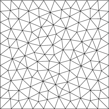
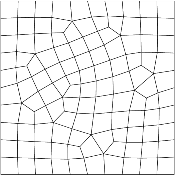
Figure 4.1. The triangular and quadrilateral meshes for example 1.

We plot convergence rate in Figure 4.2 and Figure 4.3 for the triangular and quadrilateral meshes, respectively. It is clear that the method converges in the energy norm with rate $m$ and converges in $L^{2}$ norm with rate $m+1$, where $m$ is the reconstruction order, which is consistent with the theoretical prediction in Theorem 3.1. The numerical errors and convergence rates are also presented in Table 4.1 and Table 4.2 for the triangular and quadrilateral meshes, respectively.

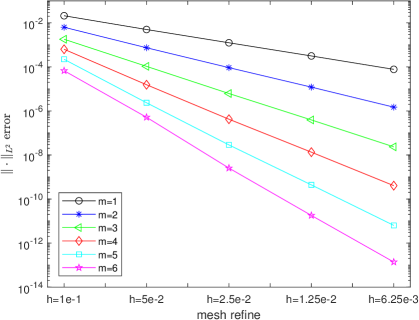
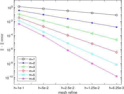
Figure 4.2. The convergence rate in $L^{2}$ norm (left) and the energy norm (right) for different reconstruction order $m$ on triangular meshes for Example 1.

		h=1.0e-1	5.0e-2	2.5e-2	1.25e-2	6.25e-3
$m$	Norms	error	error	error	error	error	Rate
	$\|\,u-u_{h}\,\|_{L^{2}}$	2.10e-02	4.98e-03	1.24e-03	3.14e-04	7.73e-05	2.02
1	$\|\!|\,u-u_{h}\,\|\!|$	1.23e+00	6.10e-01	3.06e-01	1.52e-01	7.58e-02	1.01
	$\|\,u-u_{h}\,\|_{L^{2}}$	6.32e-03	7.40e-04	9.26e-05	1.20e-05	1.48e-06	3.00
2	$\|\!|\,u-u_{h}\,\|\!|$	3.56e-01	8.91e-02	2.25e-02	5.87e-03	1.45e-03	1.98
	$\|\,u-u_{h}\,\|_{L^{2}}$	1.80e-03	1.05e-04	6.18e-06	3.91e-07	2.34e-08	4.05
3	$\|\!|\,u-u_{h}\,\|\!|$	1.01e-01	1.22e-02	1.47e-03	1.85e-04	2.25e-05	3.03
	$\|\,u-u_{h}\,\|_{L^{2}}$	6.32e-04	1.54e-05	4.21e-07	1.34e-08	4.05e-10	5.13
4	$\|\!|\,u-u_{h}\,\|\!|$	3.38e-02	1.81e-03	9.93e-05	6.27e-06	3.81e-07	4.10
	$\|\,u-u_{h}\,\|_{L^{2}}$	2.21e-04	2.35e-06	2.86e-08	4.39e-10	6.36e-12	6.25
5	$\|\!|\,u-u_{h}\,\|\!|$	1.28e-02	3.15e-04	7.33e-06	2.25e-07	6.38e-09	5.23
	$\|\,u-u_{h}\,\|_{L^{2}}$	6.73e-05	5.16e-07	2.54e-09	1.80e-11	1.38e-13	7.25
6	$\|\!|\,u-u_{h}\,\|\!|$	4.20e-03	8.45e-05	7.22e-07	9.23e-09	1.39e-10	6.28

Table 4.1. Errors on the triangular meshes for Example 1.

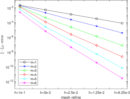
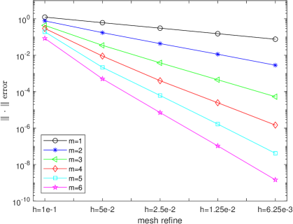
Figure 4.3. Convergence rate in $L^{2}$ norm (left) and the energy norm (right) for different reconstruction order $m$ on quadrilateral meshes for Example 1.

		h=1.0e-1	5.0e-2	2.5e-2	1.25e-2	6.25e-3
$m$	Norms	error	error	error	error	error	Rate
	$\|\,u-u_{h}\,\|_{L^{2}}$	3.30e-02	7.41e-03	1.78e-03	4.47e-04	1.06e-04	2.01
1	$\|\!|\,u-u_{h}\,\|\!|$	1.51e+00	6.93e-01	3.48e-01	1.73e-01	8.44e-02	1.01
	$\|\,u-u_{h}\,\|_{L^{2}}$	1.88e-02	2.01e-03	2.37e-04	3.05e-05	3.77e-06	3.06
2	$\|\!|\,u-u_{h}\,\|\!|$	7.70e-01	1.73e-01	4.35e-02	1.13e-02	2.83e-03	2.01
	$\|\,u-u_{h}\,\|_{L^{2}}$	1.43e-02	4.48e-04	2.25e-05	1.27e-06	7.47e-08	4.35
3	$\|\!|\,u-u_{h}\,\|\!|$	4.35e-01	3.48e-02	3.82e-03	4.51e-04	5.30e-05	3.22
	$\|\,u-u_{h}\,\|_{L^{2}}$	1.25e-02	1.16e-04	2.40e-06	7.68e-08	2.23e-09	5.53
4	$\|\!|\,u-u_{h}\,\|\!|$	2.95e-01	9.01e-03	4.00e-04	2.47e-05	1.46e-06	4.37
	$\|\,u-u_{h}\,\|_{L^{2}}$	6.31e-03	2.56e-05	3.66e-07	5.32e-09	6.53e-11	6.52
5	$\|\!|\,u-u_{h}\,\|\!|$	1.93e-01	2.16e-03	6.16e-05	1.66e-06	4.15e-08	5.46
	$\|\,u-u_{h}\,\|_{L^{2}}$	2.37e-03	6.44e-06	4.32e-08	3.56e-10	2.65e-12	7.36
6	$\|\!|\,u-u_{h}\,\|\!|$	8.43e-02	5.07e-04	7.10e-06	1.06e-07	1.45e-09	6.38

Table 4.2. Errors on the quadrilateral mesh for Example 1.

Example 2. This example is taken from [11, Example 4.1]. We consider the Dirichlet boundary value problem in the unit square $(0,1)^{2}$ with the exact solution

$$u(x,y)=x^{3}y^{2}+x\sin(2\pi xy)\sin(2\pi y).$$

The coefficient matrix $A$ is taken as

$$A(x,y)=\begin{pmatrix}(x+1)^{2}+y^{2}&-xy\\ -xy&(x+1)^{2}\end{pmatrix}.$$

The force $f$ is then determined by the equation (4.1). We solve this problem over a sequence of hexagonal meshes as shown in Figure 4.4, which are generated by a Voronoi tessellation. The mesh contains elements with different shapes such as hexagons, pentagons, and quadrilaterals. The complexity of complicate element shape does not bring in extra difficulties in implementation. The errors and convergence rate are reported in Table 4.3 and Figure 4.5, respectively, which are agreed with the theoretical prediction.

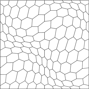
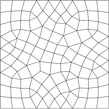
Figure 4.4. The hexagonal mesh and the mixed mesh for Example 2 and Example 3.

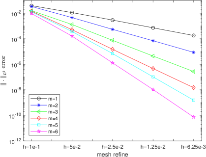
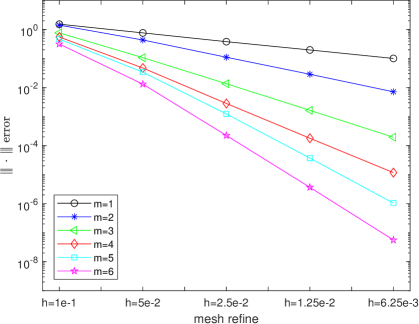
Figure 4.5. The convergence rate in $L^{2}$ norm (left) and the energy norm (right) for different reconstruction order $m$ over hexagonal meshes for Example 2.

		N=1.15e+2	4.30e+2	1.66e+3	6.52e+3	2.58e+4
$m$	Norms	error	error	error	error	error	Rate
	$\|\,u-u_{h}\,\|_{L^{2}}$	3.91e-02	1.11e-02	2.87e-03	7.17e-04	1.79e-04	1.95
1	$\|\!|\,u-u_{h}\,\|\!|$	1.53e+00	7.67e-01	3.82e-01	1.97e-01	1.01e-01	0.98
	$\|\,u-u_{h}\,\|_{L^{2}}$	3.35e-02	4.50e-03	5.42e-04	6.94e-05	8.57e-06	2.99
2	$\|\!|\,u-u_{h}\,\|\!|$	1.41e+00	4.36e-01	1.11e-01	2.87e-02	7.15e-03	1.92
	$\|\,u-u_{h}\,\|_{L^{2}}$	1.58e-02	1.29e-03	7.48e-05	4.41e-06	2.69e-07	3.99
3	$\|\!|\,u-u_{h}\,\|\!|$	7.67e-01	1.07e-01	1.35e-02	1.64e-03	1.94e-04	2.99
	$\|\,u-u_{h}\,\|_{L^{2}}$	1.42e-02	5.09e-04	1.48e-05	4.61e-07	1.47e-08	4.99
4	$\|\!|\,u-u_{h}\,\|\!|$	5.53e-01	4.73e-02	2.83e-03	1.79e-04	1.17e-05	3.91
	$\|\,u-u_{h}\,\|_{L^{2}}$	1.28e-02	3.65e-04	6.89e-06	1.02e-07	1.54e-09	5.77
5	$\|\!|\,u-u_{h}\,\|\!|$	4.68e-01	3.40e-02	1.23e-03	3.71e-05	1.04e-06	4.74
	$\|\,u-u_{h}\,\|_{L^{2}}$	9.45e-03	1.59e-04	1.28e-06	1.04e-08	7.33e-11	6.78
6	$\|\!|\,u-u_{h}\,\|\!|$	3.17e-01	1.31e-02	2.23e-04	3.65e-06	5.58e-08	5.67

Table 4.3. Errors on the hexagonal meshes for Examples 2. $N$ is the number of the total degrees of freedom.

Example 3. We consider a Neumann boundary value problem in the unit square with the exact solution

$$u(x,y)=\exp\left(\frac{x^{2}+y^{2}}{2}\right)+\sin(2\pi(x+y))\sin(2\pi y),$$

and we take the coefficients matrix as

$$A(x,y)=\begin{pmatrix}3+\cos(2\pi x)&x-y\\ x-y&3-\sin(2\pi y)\end{pmatrix}.$$

The meshes are generated by Gmsh [23] again, which contains both triangles and quadrilaterals as shown in Figure 4.4. In this example, the sampling points are randomly selected inside the element instead of the element barycenters. We perturb each barycenter with a uniform distribution random vector $\xi\in\mathbb{R}^{2}$ with $\left\lvert\xi\right\rvert=0.1h_{K}$, which guarantees the perturbed sampling points are still located in the interior of the corresponding element. We show in Figure 2.1 an example of the perturbed sampling points.

Errors are given in Table 4.4 and Figure 4.6. Again we achieved the same convergence rates as the previous examples. This indicates that the method is robust with respect to the perturbation of the sampling points as shown in Lemma 2.3.

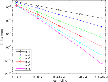
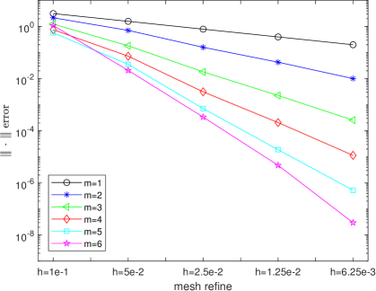
Figure 4.6. The convergence rate in $L^{2}$ norm (left) and the energy norm (right) for different $m$ for Example 3.

		N=1.29e+2	5.10e+2	2.33e+3	9.24e+3	3.80e+4
$m$	Norms	error	error	error	error	error	Rate
	$\|\,u-u_{h}\,\|_{L^{2}}$	6.66e-02	1.48e-02	3.47e-03	8.27e-04	2.01e-04	2.07
1	$\|\!|\,u-u_{h}\,\|\!|$	3.35e+00	1.57e+00	8.44e-01	4.04e-01	2.02e-01	0.99
	$\|\,u-u_{h}\,\|_{L^{2}}$	4.76e-02	6.68e-03	7.00e-04	9.29e-05	1.08e-05	3.04
2	$\|\!|\,u-u_{h}\,\|\!|$	2.17e+00	7.12e-01	1.59e-01	4.28e-02	1.00e-02	1.96
	$\|\,u-u_{h}\,\|_{L^{2}}$	3.11e-02	1.81e-03	8.04e-05	4.85e-06	2.69e-07	4.22
3	$\|\!|\,u-u_{h}\,\|\!|$	1.24e+00	1.82e-01	1.82e-02	2.25e-03	2.56e-04	3.08
	$\|\,u-u_{h}\,\|_{L^{2}}$	1.63e-02	7.26e-04	1.42e-05	4.63e-07	1.26e-08	5.12
4	$\|\!|\,u-u_{h}\,\|\!|$	7.55e-01	7.29e-02	3.12e-03	2.06e-04	1.13e-05	4.05
	$\|\,u-u_{h}\,\|_{L^{2}}$	1.27e-02	3.31e-04	2.95e-06	3.84e-08	5.62e-10	6.19
5	$\|\!|\,u-u_{h}\,\|\!|$	5.73e-01	3.54e-02	7.10e-04	1.88e-05	5.23e-07	5.10
	$\|\,u-u_{h}\,\|_{L^{2}}$	1.76e-02	2.09e-04	1.21e-06	8.66e-09	2.99e-11	7.28
6	$\|\!|\,u-u_{h}\,\|\!|$	1.10e+00	2.07e-02	3.36e-04	4.74e-06	2.97e-08	6.24

Table 4.4. Errors and convergence rates for Example 3.

5. Conclusions

Using a least-squares patch reconstruction, we construct a new discontinuous finite element space on polygonal mesh, which together with the variational formulation of DG method gives a new approximation method for partial differential equations. A novelty of this method is that arbitrary-order accuracy has been achieved with only one degree of freedom on each element, while the shape of the element may be arbitrary. Optimal error estimates have been proved and a variety of numerical examples demonstrate the superior performance of the method. It would be interesting to consider the $h-m$ version of the proposed method and the corresponding adaptive refinement strategy, and to consider the choice of the interior penalty parameter that allow for edge/face degeneration as in [14], which is key for implementation the method on more general polytopic mesh. Moreover, the assumption on the element patch may be further weakened, which may render more flexibility for the method. We shall leave all these issues to further exploration.

References

- [1] R.A. Adams and J.J.F. Fournier, Sobolev Spaces, second ed., Pure and Applied Mathematics (Amsterdam), vol. 140, Elsevier/Academic Press, Amsterdam, 2003. MR 2424078
- [2] P.F. Antonietti, S. Giani, and P. Houston, -version composite discontinuous Galerkin methods for elliptic problems on complicated domains, SIAM J. Sci. Comput. 35 (2013), no. 3, A1417–A1439. MR 3061474
- [3] D.N. Arnold, An interior penalty finite element method with discontinuous elements, SIAM J. Numer. Anal. 19 (1982), no. 4, 742–760. MR 664882
- [4] D.N. Arnold, F. Brezzi, B. Cockburn, and L.D. Marini, Unified analysis of discontinuous Galerkin methods for elliptic problems, SIAM J. Numer. Anal. 39 (2001/02), no. 5, 1749–1779. MR 1885715
- [5] T.J. Barth and M.G. Larson, A posteriori error estimates for higher order Godunov finite volume methods on unstructured meshes, Finite volumes for complex applications, III (Porquerolles, 2002), Hermes Sci. Publ., Paris, 2002, pp. 27–49. MR 2007403
- [6] F. Bassi, L. Botti, and A. Colombo, Agglomeration-based physical frame dG discretization: an attempt to be mesh free, Math. Models Methods Appl. Sci. 24 (2014), 1495–1539.
- [7] F. Bassi, L. Botti, A. Colombo, and S. Rebay, Agglomeration-based discontinuous galerkin discretization of Euler and Navier-Stokes equations, Comput. Fluids 61 (2012), 77–85.
- [8] L. Beirão da Veiga, K. Lipnikov, and G. Manzini, The Mimetic Finite Difference Method for Elliptic Problems, MS&A. Modeling, Simulation and Applications, vol. 11, Springer, Cham, 2014. MR 3135418
- [9] S.C. Brenner and L. R. Scott, The Mathematical Theory of Finite Element Methods, third ed., Texts in Applied Mathematics, vol. 15, Springer, New York, 2008. MR 2373954
- [10] F. Brezzi, A. Buffa, and K. Lipnikov, Mimetic finite differences for elliptic problems, ESAIM Numer. Anal. 43 (2009), 277–295.
- [11] F. Brezzi, K. Lipnikov, and V. Simoncini, A family of mimetic finite difference methods on polygonal and polyhedral meshes, Math. Models Methods Appl. Sci. 15 (2005), no. 10, 1533–1551. MR 2168945
- [12] A. Cangiani, Z.N. Dong, E.H. Georgoulis, and P. Houston, hp-version discontinuous galerkin methods for advection-diffusion-reaction problems on polytopic meshes, ESAIM Math. Model. Numer. Anal. 50 (2016), 699–725.
- [13] by same author, hp-Version Discontinuous Galerkin Methods on Polygonal and Polyhedral Meshes, SpringerBriefs in Mathematics, Springer International Publishing AG, 2017.
- [14] A. Cangiani, E.H. Georgoulis, and P. Houston, -version discontinuous Galerkin methods on polygonal and polyhedral meshes, Math. Models Methods Appl. Sci. 24 (2014), no. 10, 2009–2041. MR 3211116
- [15] P. G. Ciarlet, The Finite Element Method for Elliptic Problems, North-Holland, Amsterdam, 1978.
- [16] B. Cockburn, J. Gopalakrishnan, and R. Lazarov, Unified hybridization of discontinuous Galerkin, mixed, and continuous Galerkin methods for second order elliptic problems, SIAM J. Numer. Anal. 47 (2009), 1319–1365.
- [17] B. Cockburn, G.E. Karniadakis, and C.-W. Shu, The development of discontinuous Galerkin methods, Discontinuous Galerkin methods (Newport, RI, 1999), Lect. Notes Comput. Sci. Eng., vol. 11, Springer-Verlag, Berlin Heildelberg, 2000, pp. 3–50. MR 1842161
- [18] S. Dekel and D. Leviatan, The Bramble-Hilbert lemma for convex domains, SIAM J. Math. Anal. 35 (2004), 1203–1212.
- [19] D.A. Di Pierto and A. Ern, Mathematical Aspects of Discontinuous Galerkin Methods, Mathématique & Applications, vol. 69, Springer-Verlag, Berkin Heudelberg, 2012.
- [20] by same author, Arbitrary-order mixed methods for heterogeneous anisotropic diffusion on general meshes, IMA J. Numer. Anal. 37 (2017), 40–63.
- [21] D.A. Di Pierto, A. Ern, and S. Lemaire, An arbitrary-order and compact-stencil discretization of diffusion on general meshes based on local reconstruction operators, Comput. Mathods Appl. Math. 14 (2014), 461–472.
- [22] T. Dupont and L.R. Scott, Polynomial approximation of functions in Sobolev spaces, Math. Comp. 34 (1980), no. 150, 441–463. MR 559195
- [23] C. Geuzaine and J.-F. Remacle, Gmsh: A 3-D finite element mesh generator with built-in pre- and post-processing facilities, Internat. J. Numer. Methods Engrg. 79 (2009), no. 11, 1309–1331. MR 2566786
- [24] P. Grisvard, Elliptic Problems in Nonsmooth Domains, Classics in Applied Mathematics, vol. 69, Society for Industrial and Applied Mathematics (SIAM), Philadelphia, PA, 2011. MR 3396210
- [25] J.K. Hampshire, Topping B.H.V., and Chan H.C., Three node triangular bending elements with one degree of freedom per node, Engrg. Comput. 9 (1992), no. 1, 49–62.
- [26] J.S. Hesthaven and T. Warburton, Nodal Discontinuous Galerkin Methods, Texts in Applied Mathematics, vol. 54, Springer, New York, 2008, Algorithms, Analysis, and Applications. MR 2372235
- [27] K. Larsson and M.G. Larson, Continuous piecewise linear finite elements for the Kirchhoff-Love plate equation, Numer. Math. 121 (2012), 65–97.
- [28] R. Li, P.-B. Ming, Z.Y. Sun, F.Y. Yang, and Z.J. Yang, A discontinuous Galerkin method by patch reconstruction for biharmonic problem, 2017, preprint, Arxiv, 2117041.
- [29] R. Li, P.-B. Ming, and F.Y. Tang, An efficient high order heterogeneous multiscale method for elliptic problems, Multiscale Model. Simul. 10 (2012), no. 1, 259–283. MR 2902607
- [30] K. Lipnikov, D. Vassilev, and I. Yotov, Discontinuous Galerkin and mimetic finite difference methods for coupled Stokes-Darcy flows on polygonal and polyhedral grids, Numer. Math. 126 (2013), 1–40.
- [31] I. Mozolevski and E. Süli, A priori error analysis for the -version of the discontinuous Galerkin finite element method for the biharmonic equation, Comput. Methods Appl. Math. 3 (2003), no. 4, 596–607. MR 2048235
- [32] L. Mu, J.P. Wang, Y.Q. Wang, and X. Ye, Interior penalty discontinuous Galerkin method on very general polygonal and polyhedral meshes, J. Comput. Appl. Math. 255 (2014), 432–440. MR 3093433
- [33] F.J. Narcowich, J.D. Ward, and H. Wendland, Sobolev bounds on functions with scattered zeros, with applications to radial basis function surface fitting, Math. Comp. 74 (2005), no. 250, 743–763. MR 2114646
- [34] R.A. Nay and S. Utku, An alternative for the finite element method, Variational Methods in Engineering, vol. 1, University of Southampton, 1972.
- [35] E. Oñate and M. Cervera, Derivation of thin plate bending elements with one degree of freedom per node: a simple three node triangle, Engrg. Comput. 10 (1993), no. 6, 543–561.
- [36] R. Phaal and C. R. Calladine, A simple class of finite elements for plate and shell problems. II: An element for thin shells, with only translational degrees of freedom, Internat. J. Numer. Methods Engrg. 35 (1992), no. 5, 979–996.
- [37] W.H. Reed and T.R. Hill, Triangular mesh methods for the neutron transport equation, 1973, Tech. Report LA-UR-73-479, Los Alamos Scientific Laboratory.
- [38] L. Reichel, On polynomial approximation in the uniform norm by the discrete least squares method, BIT 26 (1986), no. 3, 349–368. MR 856079
- [39] N. Sukumar and A. Tabarraei, Conforming polygonal finite elements, Internat. J. Numer. Methods Engrg. 61 (2004), no. 12, 2045–2066. MR 2101599
- [40] D.O. Sullivan, Exploring spatial process dynamics using irregular cellular automaton models, Geographical Analysis 33 (2001), 1–18.
- [41] V. Venkatakrishnan, Convergence to steady state solutions of the Euler equations on unstructured grids with limiters, J. Comput. Phys. 118 (1995), no. 1, 120–130.
- [42] H. Wendland, Scattered Data Approximation, Cambridge Univeristy Press, Cambridge, 2005.
- [43] D.R. Wilhelmsen, A Markov inequality in several dimensions, J. Approximation Theory 11 (1974), 216–220. MR 0352826
- [44] D. Wirasaet, E.J. Kubatko, C.E. Michoski, S. Tanaka, J.J. Westerink, and C. Dawson, Discontinuous Galerkin methods with nodal and hybrid modal/nodal triangular, quadrilateral, and polygonal elements for nonlinear shallow water flow, Comput. Methods Appl. Mech. Engrg. 270 (2014), 113–149.
- [45] S. Yamakawa and K. Shimada, Converting a tetrahedral mesh to a prism-tetrahedral hybrid mesh for FEM accuracy and efficiency, Internat. J. Numer. Methods Engrg. 80 (2009), 2099–2129.