Measurement of the lifetime of the state in atomic cesium using asynchronous gated detection
Abstract
We report a measurement of the lifetime of the cesium state using time-correlated single-photon counting spectroscopy in a vapor cell. We excite the atoms using a Doppler-free two-photon transition from the ground state, and detect the 1.47 m photons from the spontaneous decay of the to the state. We use a gated single photon detector in an asynchronous mode, allowing us to capture the fluorescence profile for a window much larger than the detector gate length. Analysis of the exponential decay of the photon count yields a lifetime of 48.28 0.07 ns, an uncertainty of 0.14%. These measurements provide sensitive tests of theoretical models of the Cs atom, which play a central role in parity violation measurements.
pacs:
32.70.CsPrecision laboratory measurements of electric dipole (E1) matrix elements are critical for the advancement of atomic parity violation (PV) studies in several regards: Precise models of atomic structure are required to extract the weak charge from any measurement of the PV transition moment; E1 matrix elements are included explicitly in the perturbative expansion for the PV moment; and measurements of the PV amplitude are always carried out relative to a different optical transition amplitude, such as a Stark-induced amplitude. Thus, we require precise determinations of electric dipole matrix elements, through a variety of laboratory measurements, and detailed comparison with ab initio theoretical results.
The most precise determination of a PV moment in any atomic system is that of the transition in cesium, carried out by Wood et al. in 1997 Wood et al. (1997). In the past 30 years, several advances in models of the atomic structure of the cesium atom Dzuba et al. (1989a, b); Blundell et al. (1992); Dzuba et al. (1997); Safronova et al. (1999); Derevianko (2000); Dzuba and Flambaum (2000); Dzuba et al. (2002); Porsev et al. (2009, 2010); Dzuba et al. (2012), and measurements of key transition amplitudes Bouchiat, M.A. et al. (1984); Tanner et al. (1992); Young et al. (1994); Hoeling et al. (1996); DiBerardino et al. (1998); Rafac and Tanner (1998); Rafac et al. (1999); Vasilyev et al. (2002); Amini and Gould (2003); Zhang et al. (2013); Antypas and Elliott (2013a, b); Toh et al. (2014); Patterson et al. (2015); Gregoire et al. (2015) have been reported. The uncertainty in the E1 transition moment is presently one of the primary contributors, along with the matrix element, to the uncertainty in the PV moment for the transition Porsev et al. (2010); Antypas and Elliott (2013a). Similarly, the uncertainties in and are primary contributors to the uncertainty of the scalar Stark polarizability for the transition Vasilyev et al. (2002); Antypas and Elliott (2013a).
In this paper we present our measurement of the lifetime of the cesium state using an asynchronous time-correlated single-photon counting (TCSPC) technique. By measuring the lifetime of the 7s state, we indirectly measure the matrix elements named above. We find a lifetime value of 48.28 0.07 ns, in good agreement with the previous measurement by Bouchiat et al. Bouchiat, M.A. et al. (1984), but with much smaller uncertainty, and in agreement with several theoretical determinations Dzuba et al. (1989b); Blundell et al. (1992); Dzuba et al. (1997); Safronova et al. (1999); Dzuba et al. (2002); Porsev et al. (2010). This work paves the way to reducing the uncertainty of the PV transition amplitude and Stark polarizability, and complements progress we are making toward a new atomic PV measurement in cesium Choi and Elliott (2016); Antypas and Elliott (2013b).
Cesium atoms in the state can spontaneously decay through the or states, which subsequently decay to the ground state, as shown in Fig. 1.
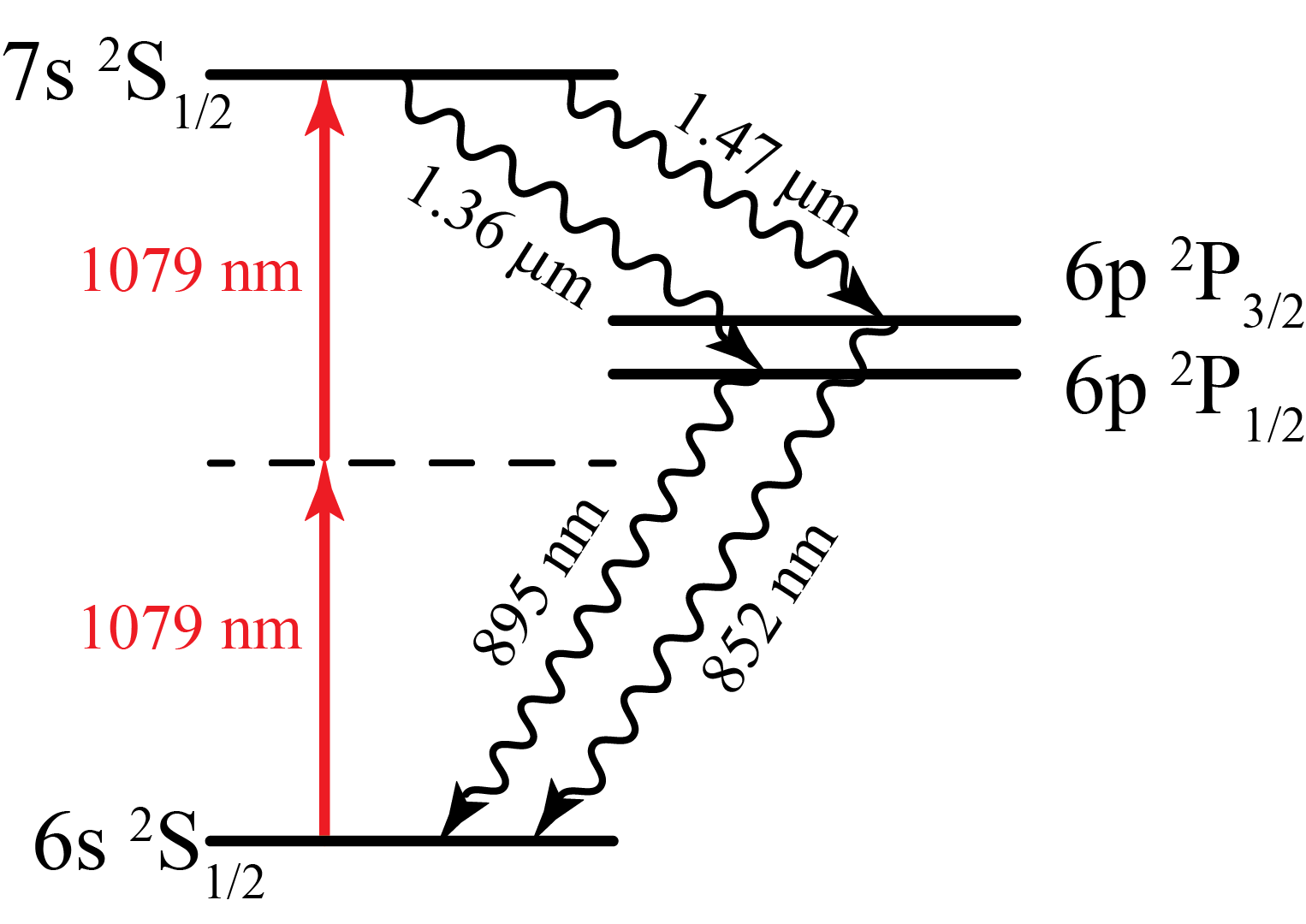
The total decay rate of the excited state is written as the sum of transition rates to these two intermediate states
| (1) |
where is the lifetime of the state, and are the transition frequencies of the and transitions, respectively, is the angular momentum of the upper state, is the fine-structure constant, and is the speed of light. Once the lifetime of the state is measured, only the ratio of matrix elements, , is needed to extract the individual matrix elements. This ratio is reliably calculated by theory and very consistent across different theoretical calculations Dzuba et al. (1989b); Blundell et al. (1992); Dzuba et al. (1997); Safronova et al. (1999).
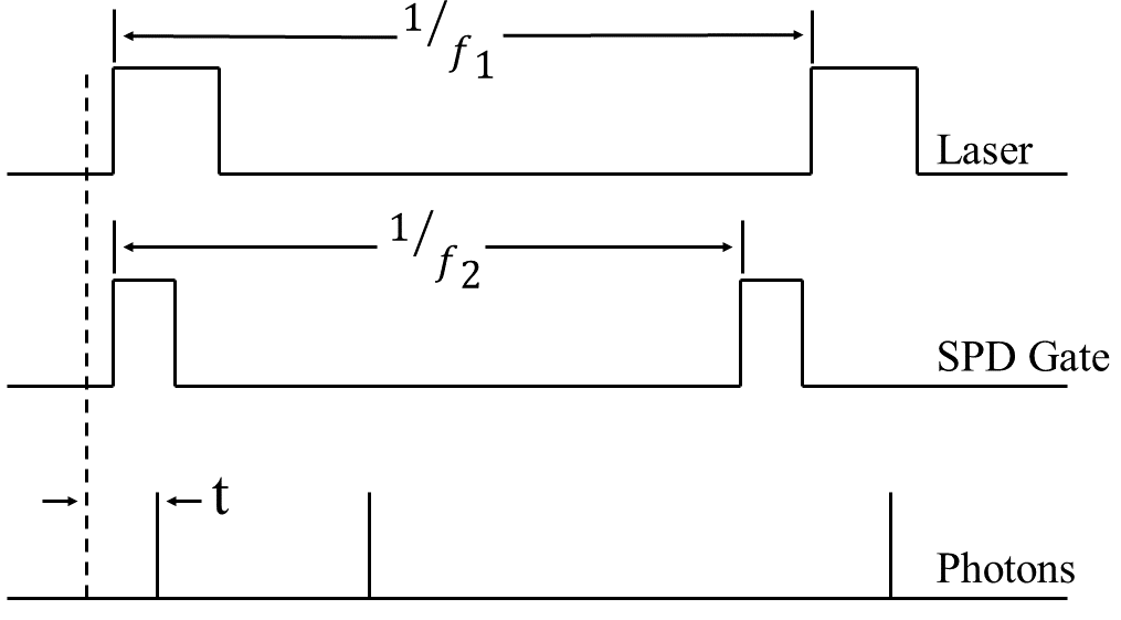
TCSPC has been used to accurately measure atomic excited state lifetimes in Cs (Hoeling et al., 1996; Young et al., 1994; DiBerardino et al., 1998), Fr (Zhao et al., 1997; Simsarian et al., 1998; Gomez et al., 2005a) and Rb (Sheng et al., 2008; Gomez et al., 2005b). A train of laser pulses repeatedly excites the atoms, and a detector records the exponential decay of fluorescence photons from the excited atoms. We introduce an asynchronous detection scheme in order to collect the fluorescence for a measurement window much longer than the gate duration of our gated single photon detector (SPD), and to reduce the impact of any possible temporal variations of the detector efficiency over the measurement window. The key to the asynchronous detection scheme is to cycle the laser excitation pulses and gated-SPD at different frequencies, and , respectively, as illustrated in Fig. 2. This causes varying delay times between the beginning of the measurement window (of duration ) and the SPD gate, which effectively causes the SPD gate pulse to repetitively scan across the full measurement window. When repeated over many cycles, the result is a flat response of the detector in time, comparable to using a free-running detector Tosi et al. (2013).
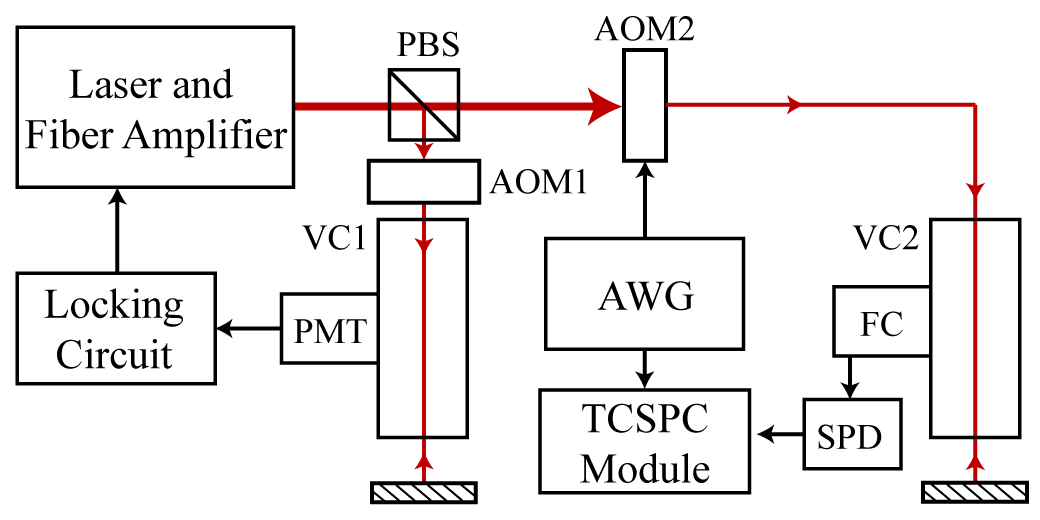
We show a schematic of our experimental setup in Fig. 3. The excitation laser is a home-made 1079 nm external cavity diode laser (ECDL), coupled into a fiber amplifier to amplify the optical power to 4 W, and split along two paths using a polarizing beam splitter (PBS) cube. We use the first of these beams to lock the laser frequency to the two-photon resonance frequency, and the second to carry out the lifetime measurements. The first beam passes through an acousto-optic modulator (AOM) driven by a constant-amplitude 90 MHz signal. We direct the first-order diffracted beam to a heated vapor cell (VC1), where a photomultiplier tube (PMT) picks up atomic fluorescence at 852 nm. This signal is processed and fed back to the laser frequency control to stabilize the laser frequency to the cesium transition ( is the total angular momentum, electron spin plus nuclear spin). We direct the second beam from the PBS to a second AOM, which is also driven at 90 MHz. The rf power driving AOM2 is pulsed on for 250 ns at a repetition rate of MHz. This pulsed beam is focused into a second heated cesium vapor cell (VC2) in a nearly-counter-propagating geometry for Doppler-free two-photon excitation (for enhancement of the signal) of the state
We filter the fluorescence at 1.47 m from this cell using a long-pass filter to reduce unwanted background (scattered laser light, other fluorescence components, and room lights, for example), and use a commercial fiber collimator to couple the fluorescence light into a m single-mode fiber. We choose to detect this fluorescence line for its reduced susceptibility to radiation trapping effects, its time dependence as a simple single exponential (in contrast to the double exponential of Hoeling et al. (1996); Gomez et al. (2005a); Sheng et al. (2008); Gomez et al. (2005b)) and its large branching ratio, compared to the 1.36 m line. The collection optics allows us to image decaying atoms within an area of m diameter. This detection volume is much greater than the region excited by the laser, and much larger than the 10 m distance traveled by an average velocity atom within one lifetime . The fiber transmits the fluorescence light to an Aurea Technology InGaAs gated avalanche single photon detector.
For accurate timing of photon arrivals, we use a HydraHarp 400 TCSPC module with a specified timing uncertainty of 12 ps. An arbitrary waveform generator (AWG) produces the start pulse for the TCSPC module, indicating the start of the 800 ns long measurement window. The AWG also generates the 90 MHz rf modulation pulse for driving AOM2, which generates the train of optical excitation pulses sent to VC2. We gate the SPD on for 40 ns at a slightly different frequency (where Hz). The TCSPC module registers the arrival time of a SPD pulse generated by the 1.47 m fluorescence photon arriving within a gate pulse. The precision of the lifetime measurement relies on the accuracy of the TCSPC timing module, but not on that of the frequency sources.
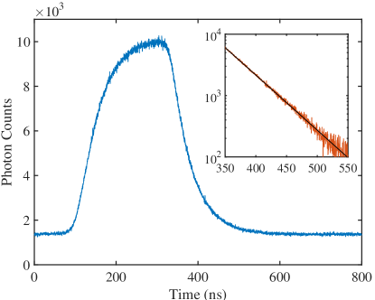
We show an example of the histogram of photon counts vs. in Fig. 4. In this figure, the ordinate represents the number of fluorescence photons detected in the i-th bin over the course of a 1 hour data run, where each bin is of duration 256 ps. The laser turns on at ns in this plot, and the fluorescence count approaches a steady-state value of counts per bin over the course of a few excited state lifetimes. This corresponds to a photon incidence rate (without gating) of per second, or the probability of detecting a photon within a 40 ns window of 0.8. The laser then turns off at 320 ns, and the signal drops, approaching a baseline value which primarily represents the detector dark noise counts. The noise level of our signal is consistent with the shot noise limit.
We apply two corrections to the raw data before determining the lifetime . The first is for pile-up error, in which we account for the probability that a second photon arrives within the 40 ns gated detection window. The correction that we apply in the asynchronous measurement scheme differs from the typical pile-up error corrections described, for example, in Gomez et al. (2005b); Simsarian et al. (1998); Sheng et al. (2008). The probability of detecting a photon within the 40 ns window centered on the i-th bin of the data set is approximately:
| (2) |
where is the total number of laser pulse repetitions (typically ), and is the duty cycle of the SPD gate. We make sure that during peak fluorescence (when the laser pulse is on) to keep any needed corrections small. For any gate pulse in which we detect a fluorescence photon, the probability of there being a second photon within that window is . This second photon is not detected, so we must multiply each point within the data set by .
We must also apply a correction to the data to account for the detector dead time. Because the detector dead time (1 s) is longer than the timing window (0.8 s), after a photon is detected, the gated-SPD is not ready to detect any photons during the next laser pulse cycle. We chose the frequency as a compromise between rapid data collection rates and long duration measurement windows, 50 ns. This necessitates an additional correction to the raw data of . In total, these two corrections alter the fitted lifetime by .
We fit an exponential function of the form
| (3) |
to the falling edge of the data to extract the lifetime of the 7s state, . Here, is the amplitude of the exponential and is the background photon count. We show an example of data and the fitted function on a semi-log plot in the inset of Fig. 4. The laser pulse has finite turn-off time, which we measured to be 20 ns (). This produces some ambiguity regarding the appropriate range of data to include in the fits, as the fluorescence decay follows an exponential only when the laser has completely turned off. We run fits to the data for a range of starting truncation points ns, but use a fixed ending truncation point at 800 ns. For each individual dataset, we determine the lifetime from the mean of these fitted lifetimes. The statistical uncertainties of these fits do not vary much across this 20 ns range, so we use the statistical uncertainty of the middle value, which we add in quadrature to the standard deviation over this range of lifetimes (the truncation error) to determine the uncertainty for each dataset. This effectively adds truncation error into our statistical uncertainty value. For most of the data sets, the truncation error is of the statistical uncertainty.
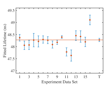
We show a plot of the 16 different measurement results used to calculate the final value of the lifetime in Fig. 5. Fourteen 1 hour long data sets and two overnight data sets of 10 hours (labeled 9 and 10 in Fig. 5) were used to determine the final lifetime. The weighted mean of these 16 lifetimes is 48.28 0.03 ns. The reduced of the resulting fit was 2.98, suggesting that our uncertainties were not sufficiently conservative. We observed that the laser lost lock several times during runs , which could be the cause of the larger variability of the results. For lack of a clear link however, we chose to increase our statistical uncertainty by .
In order to make a measurement with high accuracy, we investigated several potential systematic effects to determine their impacts on the measurement. We verified that our measurement scheme counts photons at all times with equal probability (i.e. there is no temporal variation in the detection sensitivity) by recording the background photon counts with the laser off. We measured the lifetime at several different cell temperatures and with different applied magnetic fields to verify that there was no effect from radiation trapping, collisions, or Zeeman quantum beats. (Data sets 6 through 9 of Fig. 5 were taken at a temperature of C, with the rest taken at C. In data sets 3 through 5, a 3 G magnetic field was applied to the vapor cell in each of three orthogonal directions.) Additionally, we quantified the effect of the detector jitter, included a correction for pile-up error and addressed truncation effects. We summarize the magnitudes of these effects on our error budget in Table 1. Adding statistical and systematic errors in quadrature, our final result is 48.28 0.07 ns. We display this final result as the last point in Fig. 5.
| Error | % uncertainty |
|---|---|
| Statistical and truncation | 0.12 |
| Detection sensitivity | 0.05 |
| Radiation trapping | 0.03 |
| Time calibration | 0.03 |
| Pile-up correction | 0.02 |
| SPD detector jitter | 0.01 |
| Total uncertainty | 0.14 |
| Group | (ns) |
|---|---|
| Experimental | |
| Marek, time-resolved fluorescence, 1977 Marek (1977) | |
| Hoffnagle et al., Hanle effect, 1981 Hoffnagle et al. (1981) | |
| M. Bouchiat et al., Hanle effect, 1984 Bouchiat, M.A. et al. (1984) | |
| This work, time-resolved fluorescence | |
| Theoretical | |
| C. Bouchiat et al., semi-empirical Bouchiat et al. (1983) | 48.35 |
| Dzuba et al.,∗ 1989 Dzuba et al. (1989b) | 48.07 |
| Blundell et al.,∗ 1992 Blundell et al. (1992) | 48.56 |
| Dzuba et al.,∗ 1997 Dzuba et al. (1997) | 48.07 |
| Safronova et al.,∗ 1999 Safronova et al. (1999) | 48.42 |
| Dzuba et al.,† 2002 Dzuba et al. (2002) | 48.24 |
| Porsev et al.,† 2010 Porsev et al. (2010) | 48.33 |
We present a summary of past theoretical and experimental results in Table 2. Our final result agrees well with the last experimental result by Bouchiat et al. (Bouchiat, M.A. et al., 1984) which was based on the Hanle effect. The theory values shown in the table are calculated from the E1 matrix elements reported in these works and the measured transition energies. Our result agrees within our uncertainty with the two most recent theoretical works by Dzuba (Dzuba et al., 2002) and Porsev (Porsev et al., 2010). These works only report values of , so we estimate the ratio from the earlier theory papers Dzuba et al. (1989b); Blundell et al. (1992); Dzuba et al. (1997); Safronova et al. (1999) to derive the lifetimes listed.
In summary, we present a new lifetime measurement technique using a gated SPD in an asynchronous measurement scheme, and a new, higher precision measurement result for the lifetime of the state of cesium. This measurement technique allows us to collect data for a time window much longer than the maximum gate length of a gated SPD with uniform detection sensitivity. The scheme presented here can be used to measure atomic lifetimes with high precision. Our newly measured value of this lifetime agrees well with earlier experimental and theoretical determinations of the Cs lifetime, and improves on the experimental uncertainty by a factor of seven. The lifetime measurement result presented here tests models of the cesium atomic structure, and can be used to reduce uncertainties on the PV moment and the scalar polarizability for the transition.
This material is based upon work supported by the National Science Foundation under Grant Number PHY-1607603 and PHY-1460899. JAJ acknowledges support by Colciencias Colombia through the Francisco Jose de Caldas Conv. 529 Scholarship and Fulbright Colombia. We gratefully acknowledge useful discussions with M. Y. Shalaginov, M. S. Safronova and D. E. Leaird.
References
- Wood et al. (1997) C. S. Wood, S. C. Bennett, D. Cho, B. P. Masterson, J. L. Roberts, C. E. Tanner, and C. E. Wieman, Science 275, 1759 (1997).
- Dzuba et al. (1989a) V. Dzuba, V. Flambaum, and O. Sushkov, Physics Letters A 141, 147 (1989a).
- Dzuba et al. (1989b) V. Dzuba, V. Flambaum, A. Krafmakher, and O. Sushkov, Physics Letters A 142, 373 (1989b).
- Blundell et al. (1992) S. A. Blundell, J. Sapirstein, and W. R. Johnson, Phys. Rev. D 45, 1602 (1992).
- Dzuba et al. (1997) V. A. Dzuba, V. V. Flambaum, and O. P. Sushkov, Phys. Rev. A 56, R4357 (1997).
- Safronova et al. (1999) M. S. Safronova, W. R. Johnson, and A. Derevianko, Phys. Rev. A 60, 4476 (1999).
- Derevianko (2000) A. Derevianko, Phys. Rev. Lett. 85, 1618 (2000).
- Dzuba and Flambaum (2000) V. A. Dzuba and V. V. Flambaum, Phys. Rev. A 62, 052101 (2000).
- Dzuba et al. (2002) V. A. Dzuba, V. V. Flambaum, and J. S. M. Ginges, Phys. Rev. D 66, 076013 (2002).
- Porsev et al. (2009) S. G. Porsev, K. Beloy, and A. Derevianko, Phys. Rev. Lett. 102, 181601 (2009).
- Porsev et al. (2010) S. G. Porsev, K. Beloy, and A. Derevianko, Phys. Rev. D 82, 036008 (2010).
- Dzuba et al. (2012) V. A. Dzuba, J. C. Berengut, V. V. Flambaum, and B. Roberts, Phys. Rev. Lett. 109, 203003 (2012).
- Bouchiat, M.A. et al. (1984) Bouchiat, M.A., Guena, J., and Pottier, L., J. Physique Lett. 45, 523 (1984).
- Tanner et al. (1992) C. E. Tanner, A. E. Livingston, R. J. Rafac, F. G. Serpa, K. W. Kukla, H. G. Berry, L. Young, and C. A. Kurtz, Phys. Rev. Lett. 69, 2765 (1992).
- Young et al. (1994) L. Young, W. T. Hill, S. J. Sibener, S. D. Price, C. E. Tanner, C. E. Wieman, and S. R. Leone, Phys. Rev. A 50, 2174 (1994).
- Hoeling et al. (1996) B. Hoeling, J. R. Yeh, T. Takekoshi, and R. J. Knize, Opt. Lett. 21, 74 (1996).
- DiBerardino et al. (1998) D. DiBerardino, C. E. Tanner, and A. Sieradzan, Phys. Rev. A 57, 4204 (1998).
- Rafac and Tanner (1998) R. J. Rafac and C. E. Tanner, Phys. Rev. A 58, 1087 (1998).
- Rafac et al. (1999) R. J. Rafac, C. E. Tanner, A. E. Livingston, and H. G. Berry, Phys. Rev. A 60, 3648 (1999).
- Vasilyev et al. (2002) A. A. Vasilyev, I. M. Savukov, M. S. Safronova, and H. G. Berry, Phys. Rev. A 66, 020101 (2002).
- Amini and Gould (2003) J. M. Amini and H. Gould, Phys. Rev. Lett. 91, 153001 (2003).
- Zhang et al. (2013) Y. Zhang, J. Ma, J. Wu, L. Wang, L. Xiao, and S. Jia, Phys. Rev. A 87, 030503 (2013).
- Antypas and Elliott (2013a) D. Antypas and D. S. Elliott, Phys. Rev. A 88, 052516 (2013a).
- Antypas and Elliott (2013b) D. Antypas and D. S. Elliott, Phys. Rev. A 87, 042505 (2013b).
- Toh et al. (2014) G. Toh, D. Antypas, and D. S. Elliott, Phys. Rev. A 89, 042512 (2014).
- Patterson et al. (2015) B. M. Patterson, J. F. Sell, T. Ehrenreich, M. A. Gearba, G. M. Brooke, J. Scoville, and R. J. Knize, Phys. Rev. A 91, 012506 (2015).
- Gregoire et al. (2015) M. D. Gregoire, I. Hromada, W. F. Holmgren, R. Trubko, and A. D. Cronin, Phys. Rev. A 92, 052513 (2015).
- Choi and Elliott (2016) J. Choi and D. S. Elliott, Phys. Rev. A 93, 023432 (2016).
- Zhao et al. (1997) W. Z. Zhao, J. E. Simsarian, L. A. Orozco, W. Shi, and G. D. Sprouse, Phys. Rev. Lett. 78, 4169 (1997).
- Simsarian et al. (1998) J. E. Simsarian, L. A. Orozco, G. D. Sprouse, and W. Z. Zhao, Phys. Rev. A 57, 2448 (1998).
- Gomez et al. (2005a) E. Gomez, L. A. Orozco, A. Perez Galvan, and G. D. Sprouse, Phys. Rev. A 71, 062504 (2005a).
- Sheng et al. (2008) D. Sheng, A. Pérez Galván, and L. A. Orozco, Phys. Rev. A 78, 062506 (2008).
- Gomez et al. (2005b) E. Gomez, F. Baumer, A. D. Lange, G. D. Sprouse, and L. A. Orozco, Phys. Rev. A 72, 012502 (2005b).
- Tosi et al. (2013) A. Tosi, C. Scarcella, G. Boso, and F. Acerbi, IEEE Photonics Journal 5, 6801308 (2013).
- Marek (1977) J. Marek, Journal of Physics B: Atomic and Molecular Physics 10, L325 (1977).
- Hoffnagle et al. (1981) J. Hoffnagle, V. Telegdi, and A. Weis, Physics Letters A 86, 457 (1981).
- Bouchiat et al. (1983) C. Bouchiat, C. Piketty, and D. Pignon, Nuclear Physics B 221, 68 (1983).