Aging dynamics in quenched noisy long-range quantum Ising models

Abstract

We consider the $d$-dimensional transverse-field Ising model with power-law interactions $J/r^{d+\sigma}$ in the presence of a noisy longitudinal field with zero average. We study the longitudinal-magnetization dynamics of an initial paramagnetic state after a sudden switch-on of both the interactions and the noisy field. While the system eventually relaxes to an infinite-temperature state with vanishing magnetization correlations, we find that two-time correlation functions show aging at intermediate times. Moreover, for times shorter than the inverse noise strength $\kappa$ and distances longer than $a(J/\kappa)^{2/\sigma}$ with $a$ being the lattice spacing, we find a critical scaling regime of correlation and response functions consistent with the model A dynamical universality class with an initial-slip exponent $\theta=1$ and dynamical critical exponent $z=\sigma/2$. We obtain our results analytically by deriving an effective action for the magnetization field including the noise in a non-perturbative way. The above scaling regime is governed by a non-equilibrium fixed point dominated by the noise fluctuations.

I Introduction

The concept of universality is well established in closed classical and quantum systems in equilibrium,Cardy (1996); Sachdev (2001) and has been rigorously formulated through a number of advanced frameworks such as scaling theoryCardy (1996); Sachdev (2001); Ma (1985) and the celebrated renormalization group method.Wilson (1971a, b); Wilson and Fisher (1972); Wilson and Kogut (1974); Fisher (1974); Wilson (1975) Moreover, with the great degree of control currently available in ion-trapPorras and Cirac (2004); Kim et al. (2009); Jurcevic et al. (2014) and ultracold-atom setups,Levin et al. (2012); Yukalov (2011); Bloch et al. (2008); Greiner et al. (2002) the study of phase transitions and their effects on the nonequilibrium dynamics of closed quantum systems has become experimentally possible.

In recent years, and in no small part due to this experimental advancement, out-of-equilibrium criticality and dynamical phase transitions have become the subject of extensive theoreticalTäuber (2014); Zvyagin (2016); Heyl (2018); Mori et al. (2017) and experimentalNicklas et al. (2015); Zhang et al. (2017); Jurcevic et al. (2017); Neyenhuis et al. (2017); Fläschner et al. (2018) research. In equilibrium one is able to probe criticality only in the ground state or thermal state of the system, whereas in out-of-equilibrium systems there can be multiple instances of criticality.Hohenberg and Halperin (1977) More recently the attention has shifted to criticality in prethermal states that temporally precede the steady state,Berges et al. (2004); Kitagawa et al. (2011); Gring et al. (2012); Langen et al. (2013); van den Worm et al. (2013); Marcuzzi et al. (2013); Chiocchetta et al. (2015, 2017); Maraga et al. (2015); Sciolla and Biroli (2013) and to the long-time time-translation invariant steady state itself.Sciolla and Biroli (2010, 2011, 2013) Even though the latter has been extensively studied and is known to be connected to nonanalyticities in a dynamical analog of the free energy in mean-field models,Homrighausen et al. (2017); Lang et al. (2018) the critical exponents involved in classifying the universality of the model are directly those known from equilibrium.

Prethermal criticality, on the other hand, offers the unique possibility of studying truly out-of-equilibrium criticality, because in this case criticality is probed away from the steady state and the dynamics is not time-translation invariant. One of the most fascinating aspects of such prethermal criticality is the phenomenon of aging in systems quenched to a critical point Calabrese and Gambassi (2005). Aging occurs in the prethermal regime, before the system has relaxed into its steady state, and gives rise to a truly nonequilibrium critical exponent $\theta$ that can be extracted from the intermediate-time dynamics of the order parameter or the two-time $(s,t)$ correlation and response functions thereof. Due to the broken time-translation invariance the latter do not only depend on the time difference $t-s$, even at long times. In fact, the decay as a function of $t>s$ gets slower with larger $s$. In other words, the response of a system becomes slower with its waiting time or age $s$. This is the characteristic aging behavior shown also by structural glass and spin glasses, where even though the slow dynamics after a perturbation such as a quantum or temperature quench may be approaching an asymptotic value in single-time quantities, this does not mean that the system is approaching a stationary state.

Critical dynamics of thermal systems have been shown to exhibit such aging behavior in two-time correlation functions, indicating the absence of equilibration to a time-translation invariant stationary state.Janssen et al. (1989); Gambassi and Calabrese (2011) This type of aging has been observed also in isolated systems described by $O(N)$ models,Chiocchetta et al. (2015, 2017); Maraga et al. (2015); Sciolla and Biroli (2013) where for critical quenches the response and correlation functions at small momenta exhibit time-dependence $\propto-t(s/t)^{\theta}$ and $(st)^{2-2\theta}$, respectively, for $t\gg s$.

Recently, the investigation has been extended to open systems. A coupling to (possibly non-thermal) baths might be present, together with other wanted or unwanted sources of environmental noise. As such, a theoretical framework describing how the openness of the system affects the aging behavior is desirable. Moreover, criticality can be fundamentally different between the closed and open system version of the same model, as is for instance the case for driven-dissipative systems even in the steady stateSieberer et al. (2013). In the context of critical aging dynamics, dissipative systems, like $O(N)$ models in contact with a sub- or super-Ohmic bathGagel et al. (2014) or driven and lossy fully connected spin chains,Lang and Piazza (2016) as well as noisy models,Marino and Silva (2012); Sciolla et al. (2015) have been considered. In particular, aging has been predicted for lattice bosons in the presence of phase noiseSciolla et al. (2015) and prethermalization for short-range Ising models with a noisy transverse field.Marino and Silva (2012); Lorenzo et al. (2017)

In this work, we study the relaxation dynamics after a quench in a noisy spin system. We consider a transverse-field Ising model in $d$ spatial dimensions with power-law interactions $J/r^{d+\sigma}$ as function of distance $r$ in the presence of a longitudinal field with zero average and Gaussian Markovian fluctuations of strength $\kappa$. Starting from an initial paramagnetic state and suddenly switching on both the interactions and the longitudinal noise field, we compute the dynamics of the response and correlation functions of the longitudinal magnetization. The quantum Ising model with power-law interactions is a paradigmatic setup of condensed matter and quantum many-body physics. In addition to its simplicity, it encompasses infinitely many universality classes, including in just one dimension depending on the value of $\alpha$, and it has recently been the main protagonist in experiments on dynamical phase transitions.Zhang et al. (2017); Jurcevic et al. (2017); Fläschner et al. (2018) As shown below, it also provides a quantum mechanical spin model where combined effects of noise and quench dynamics can be studied analytically, allowing our work to provide a formalism suitable for investigating criticality in current open many-body experiments.

I.1 Summary of the main findings

i).— The two-point correlation functions for any given space-time distance $t-s$ vanish exponentially as a function of the time $(t+s)/2$ elapsed after the quench, consistent with the fact that the system reaches an infinite-temperature state.Marino and Silva (2012) However, at intermediate times we find that correlation functions computed at two times $s$ and $t>s$ remain dependent on the ratio $s/t$ as is the case for aging systems (see Fig. 5). In particular, for $J\ll\kappa$ and times $t,s<1/\kappa$ we analytically obtain the response and correlation functions (for $t>s$)

$$\langle\mathcal{M}_{\mathbf{p},t}\tilde{\mathcal{M}}_{\mathbf{p},s}\rangle\simeq -\text{i}\cos[2\mathcal{R}_{\mathbf{p}}(t-s)]-\text{i}\frac{\kappa}{4\mathcal{R}_{\mathbf{p}}}\sin[2\mathcal{R}_{\mathbf{p}}(t-s)],$$ (1)

$$\langle\mathcal{M}_{\mathbf{p},t}\mathcal{M}_{-\mathbf{p},s}\rangle\simeq \frac{4h^{2}}{\mathcal{R}_{\mathbf{p}}^{2}\left(4\mathcal{R}_{\mathbf{p}}^{2}+\kappa^{2}\right)}\Bigg{\{}2\mathcal{R}_{\mathbf{p}}\Big{(}2\mathcal{R}_{\mathbf{p}}\cos[2\mathcal{R}_{\mathbf{p}}(t-s)]-\kappa\sin[2\mathcal{R}_{\mathbf{p}}(t-s)]\Big{)}\text{e}^{-2\kappa s}-\left(4\mathcal{R}_{\mathbf{p}}^{2}+\kappa^{2}\right)\cos[2\mathcal{R}_{\mathbf{p}}(t-s)]$$

$$+\kappa\left(\kappa\cos\left[2\mathcal{R}_{\mathbf{p}}(t-s)\left(\frac{1+s/t}{1-s/t}\right)\right]+2\mathcal{R}_{\mathbf{p}}\sin\left[2\mathcal{R}_{\mathbf{p}}(t-s)\left(\frac{1+s/t}{1-s/t}\right)\right]\right)\Bigg{\}},$$ (2)

with $\mathcal{R}_{\mathbf{p}}=\sqrt{h\left(h-J_{\mathbf{p}}\right)}$, where $h$ is the transverse field strength and $J_{\mathbf{p}}$ is the Fourier transform of the interaction profile $J/r^{d+\sigma}$. In (1) $\mathcal{M}$ is the longitudinal magnetization field and $\tilde{\mathcal{M}}$ is the longitudinal response field. These two-time functions show the breaking of time-translation invariance.

ii).— For a quench to the closed-system critical point $h=J_{\mathbf{0}}$ and for times $t,s\ll 1/\kappa$ as well for large distances such that $|\mathbf{p}|a(J/\kappa)^{2/\sigma}\ll 1$ with $a$ the lattice spacing, the response and correlation functions enter an aging scaling regime consistent with the model A classHohenberg and Halperin (1977); Calabrese and Gambassi (2005)

$$\langle\mathcal{M}_{\mathbf{p},t}\tilde{\mathcal{M}}_{\mathbf{p},s}\rangle\simeq\frac{\kappa}{J}(t-s)^{\frac{2-\upsilon-z}{z}}\left(\frac{t}{s}\right)^{\theta}\!\!\!\!F_{R}\!\left(|\mathbf{p}|(t-s)^{\frac{1}{z}},\frac{s}{t}\right),$$ (3)

$$\langle\mathcal{M}_{\mathbf{p},t}\mathcal{M}_{\mathbf{-p},s}\rangle\simeq(t-s)^{\frac{2-\upsilon}{z}}\left(\frac{t}{s}\right)^{\theta-1}\!\!\!\!F_{C}\!\left(|\mathbf{p}|(t-s)^{\frac{1}{z}},\frac{s}{t}\right),$$ (4)

with

$$F_{R}(x,y)=-\frac{\text{i}y}{4\sqrt{c_{0}c_{\sigma}}x^{\sigma/2}}\sin\left(2\sqrt{c_{0}c_{\sigma}}x^{\sigma/2}\right),$$ (5)

$$F_{C}(x,y)=4\frac{c_{0}}{c_{\sigma}}\frac{1}{x^{\sigma}}$$

$$\times\left[\cos\left(2\sqrt{c_{0}c_{\sigma}}x^{\sigma/2}\frac{1+y}{1-y}\right)-\cos\left(2\sqrt{c_{0}c_{\sigma}}x^{\sigma/2}\right)\right],$$ (6)

where we have expressed time in units of $1/J$ and space in units of $a$, and with $c_{0,\sigma}$ being pure numbers. We find the following critical exponents

$$z=\frac{\sigma}{2},\;\theta=1,\;\upsilon=2-\sigma.$$ (7)

The dynamical critical exponent $z$ is the same as found in the closed system.Maghrebi et al. (2016) The above scaling regime is governed by a non-equilibrium fixed point dominated by the noise fluctuations. With the choice of our interaction potential being $1/r^{d+\sigma}$, the above results should hold in arbitrary dimensions in the weakly interacting regime $J\ll\kappa$.

I.2 Organization of paper

The rest of the paper is organized as follows. In Sec. II we present our formalism, based on the Keldysh path-integral formulation for out-of-equilibrium many-body problems, that allows us to eventually derive a Langevin vector equation, from which two-time response and correlation functions of the longitudinal magnetization and its current can be extracted. In Sec. III we present our numerical results for the two-time response and correlation functions of the longitudinal magnetization, and discuss the relaxation dynamics and aging observed therein, in addition to critical scaling behavior for quenches close to the critical point. We conclude in Sec. IV, whilst providing further details of our derivation in Appendix A.

II Formalism

Our goal is to derive an effective Langevin equation governing the post-quench dynamics of the longitudinal magnetization in presence of a noisy magnetic field. Within this semiclassical approximation, the fluctuations in the magnetization are induced only by the field noise. Upon formulating the Martin-Siggia-Rose-De Dominicis-Janssen (MSRDJ) classical actionKamenev (2011) corresponding to the above Langevin equation, we compute two-point correlators within a Gaussian approximation.

The starting point for the derivation of the Langevin equation is a Hubbard-Stratonovich (HS) decoupling of the Ising interaction term performed within a path-integral formulation of the quench problem on the closed semi-infinite time contourDanielewicz (1984) shown in Fig. 1. The decoupling is performed after mapping the spin-$1/2$ degrees of freedom to Schwinger bosons. In the absence of the noisy field, the HS decoupling would be equivalent to the usual mean-field decoupling. Here we instead include the noise non-perturbatively by solving the Dyson equation for the two-point bosonic Green’s function (GF) in a self-consistent manner.

In Sec. II.1 we begin with introducing the quantum spin model used to describe our system and its mapping to Schwinger bosons. In Sec. II.2 we then describe the path-integral formulation of the problem on a closed semi-infinite time contour. In Sec. II.3 we finally derive the Langevin equation and its corresponding MSRDJ action.

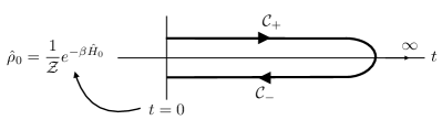
Figure 1: Closed semi-infinite time contour employed in the path-integral formulation of the quench problem studied in this work. At the initial time $t=0$ our system is in a thermal state of the non-interacting noisless Hamiltonian $H_{0}$ given in (8).

II.1 Model and Schwinger-boson mapping

We consider a transverse-field Ising model described by the Hamiltonian

$$\hat{H} =\hat{H}_{0}+\hat{V},$$ (8)

$$\hat{H}_{0} =-h\sum_{i}\hat{\sigma}^{x}_{i},$$ (9)

$$\hat{V} =-\frac{1}{2}\sum_{i\neq j}J_{ij}\hat{\sigma}^{z}_{i}\hat{\sigma}^{z}_{j}+\sum_{i}\eta_{i,t}\hat{\sigma}^{z}_{i},$$ (10)

with $J_{ij}=J/|i-j|^{d+\sigma}$ the spin-spin coupling profile, $h$ the transverse-field strength, and $\hat{\sigma}^{x,z}$ the Pauli matrices along the $x$ and $z$ directions, respectively. We add a noisy longitudinal field $\eta_{i,t}$ with zero average and Gaussian fluctuations:

$$\langle\eta_{i,t}\rangle =0,$$ (11)

$$\langle\eta_{i,t}\eta_{j,t^{\prime}}\rangle =\frac{\kappa}{2}\delta_{i,j}\delta(t-t^{\prime}),$$ (12)

with $\kappa$ a strength parameter.

We now use the Schwinger-boson representation of the Pauli spin operators,

$$\hat{\sigma}^{z} =\text{sgn}{(}\alpha)\hat{b}_{i,\alpha}^{\dagger}\hat{b}_{i,\alpha},$$ (13)

$$\hat{\sigma}^{x} =\hat{b}_{i,\alpha}^{\dagger}\hat{b}_{i,\bar{\alpha}},$$ (14)

with implied summation over spin indices, where $\hat{b}_{i\alpha}^{\left(\dagger\right)}$ is the Schwinger-boson annihilation (creation) operator on site $i$ for the two spin components $\alpha=\pm 1$ (or, equivalently in our notation, $\alpha=\uparrow\downarrow$) obeying the canonical commutation relations $[\hat{b}_{i,\alpha},\hat{b}_{j,\beta}^{\dagger}]=\delta_{i,j}\delta_{\alpha,\beta}$ and $[\hat{b}_{i,\alpha},\hat{b}_{j,\beta}]=0$. This allows us to express our Hamiltonian in the form

$$\hat{H}= -\frac{1}{2}\sum_{i\neq j}J_{ij}\text{sgn}{(}\alpha)\text{sgn}{(}\beta)\hat{b}_{i,\alpha}^{\dagger}\hat{b}_{j,\beta}^{\dagger}\hat{b}_{i,\alpha}\hat{b}_{j,\beta}$$

$$-h\sum_{i}\hat{b}_{i\alpha}^{\dagger}\hat{b}_{i\bar{\alpha}}+\sum_{i}\eta_{i,t}\text{sgn}{(}\alpha)\hat{b}_{i\alpha}^{\dagger}\hat{b}_{i\alpha}$$

$$+\sum_{i}\lambda_{i,t}\big{(}\hat{b}_{i\alpha}^{\dagger}\hat{b}_{i\alpha}-2S\big{)},$$ (15)

where we have additionally included in the last line a Lagrange multiplier $\lambda_{i,t}$ to constrain the number of bosons per site to $2S$ at all times $t$, with $S=1/2$ the spin length in our model.

II.2 Non-equilibrium path-integral formulation

We want to describe the dynamics within the following quench protocol. At $t=0$ we prepare the system in a thermal state $\hat{\rho}_{0}=\text{e}^{-\beta\hat{H}_{0}}/\mathcal{Z}$ of the non-interacting, noiseless Hamiltonian $\hat{H}_{0}$, and then let it subsequently evolve with the full Hamiltonian (8) in the presence of the noise.

In order to compute non-equilibrium GFs we adopt a path-integral formulation of the partition function on the closed semi-infinite time contourDanielewicz (1984) $\mathcal{C}:0\to\infty\to 0$ shown in Fig. 1.

After HS-decoupling of the interaction term using the auxiliary longitudinal magnetization field $\mathcal{M}$, the noise-averaged partition function reads (see Appendix A for more details)

$$\mathcal{Z}=\int\limits\mathscr{D}[\bar{\phi}^{\chi},\phi^{\chi},\mathcal{M}^{\chi},\lambda,\eta]\text{e}^{\text{i}\mathcal{S}[\bar{\phi}^{\chi},\phi^{\chi},\mathcal{M}^{\chi},\lambda,\eta]},$$ (16)

with the action given by

$$\mathcal{S}[\bar{\phi}^{\chi},\phi^{\chi},\mathcal{M}^{\chi},\lambda,\eta]= \int\limits_{0}^{\infty}\mathrm{d}t\;\sum_{\chi=\pm}\chi\sum_{i}\left(\bar{\phi}_{i,\alpha,t}^{\chi}\text{i}\partial_{t}\phi_{i,\alpha,t}^{\chi}+h\bar{\phi}_{i,\alpha,t}^{\chi}\phi_{i,\bar{\alpha},t}^{\chi}-\eta_{i,t}\text{sgn}{(}\alpha)\bar{\phi}_{i,\alpha,t}^{\chi}\phi_{i,\alpha,t}^{\chi}-\lambda_{i,t}\bar{\phi}_{i,\alpha,t}^{\chi}\phi_{i,\alpha,t}^{\chi}\right)+$$

$$+\int\limits_{0}^{\infty}\mathrm{d}t\;\sum_{\chi=\pm}\chi\sum_{i\neq j}\left(\mathcal{M}^{\chi}_{j,t}J_{ij}\text{sgn}{(}\alpha)\bar{\phi}_{i,\alpha,t}^{\chi}\phi_{i,\alpha,t}^{\chi}-\mathcal{M}^{\chi}_{i,t}\frac{J_{ij}}{2}\mathcal{M}^{\chi}_{j,t}\right)+\frac{\text{i}}{\kappa}\int\limits_{0}^{\infty}\mathrm{d}t\;\sum_{i}\eta_{i,t}^{2},$$ (17)

where $\chi=\pm$ indicates the forward ($0\to\infty$) or backward ($\infty\to 0$) branch of the contour, respectively, $\phi_{i,\alpha,t}^{\chi}$ are bosonic fields with $\bar{\phi}_{i,\alpha,t}^{\chi}$ their complex conjugate, and $\mathcal{M}_{i,t}^{\chi}$ is a real field. The noise field $\eta_{i,t}$ is a classical field and therefore its value does not depend on the contour branch.

II.3 Langevin equation and MSRDJ action

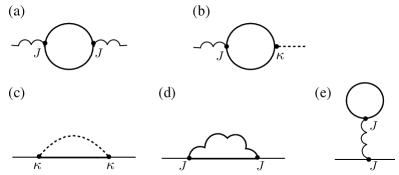
Figure 2: Diagrammatic expression of the Gaussian action for the magnetization field $\mathcal{M}$ (wiggly lines), leading to the Langevin equation (18). The dimensionless noise field $\eta/\kappa$ is indicated by a dashed line while the Schwinger boson by a solid line. The magnetization couples to the bosons with coupling constant $J_{ij}$ while the dimensionless noise field with coupling constant $\kappa$. The non-equilibrium Green’s functions are computed on the semi-infinite real-time closed contour of Fig. 1. Contour indices as well as bosonic spin indices are suppressed. The Gaussian action is defined by diagrams (a) plus (b), whereby the bosonic loops are computed using the Green’s functions dressed by the self-energy insertions (c), (d), and (e).

In order to obtain the Langevin equation describing the dynamics of the magnetization field $\mathcal{M}_{i,t}$, we perform a Keldysh rotation in (17), integrate out the classical and quantum bosonic fields $\phi^{\text{cl}(\text{q})}_{i,\alpha,t}=(\phi^{+}_{i,\alpha,t}\pm\phi^{-}_{i,\alpha,t})/\sqrt{2}$, and consider the saddle-point equation of motion up to linear order in $\mathcal{M}_{i,t}$ (see Appendix A for a detailed derivation), which reads

$$\mathcal{M}_{i,t}=-2\text{i}\int\limits_{0}^{\infty}\mathrm{d}\tau\Big{(}\sum_{l}J_{il}\mathcal{M}_{l,\tau}-\eta_{i,\tau}\Big{)}\times$$

$$\times\Big{(}\Re G_{(i,\tau),(i,t)}^{\text{K},\uparrow\uparrow}G_{(i,t),(i,\tau)}^{\text{R},\uparrow\uparrow}-\text{i}\Im G_{(i,\tau),(i,t)}^{\text{K},\uparrow\downarrow}G_{(i,t),(i,\tau)}^{\text{R},\downarrow\uparrow}\Big{)},$$ (18)

with the classical component of the magnetization field $\mathcal{M}_{i,t}\equiv\mathcal{M}_{i,t}^{\text{cl}}=(\mathcal{M}^{+}_{i,t}+\mathcal{M}^{-}_{i,t})/2$ and we have assumed our system is in the paramagnetic phase so that $G^{\uparrow\uparrow}=G^{\downarrow\downarrow}$ and $G^{\uparrow\downarrow}=G^{\downarrow\uparrow}$, with the bosonic GFs defined as $\text{i}G_{(j,t),(j^{\prime},t^{\prime})}^{\text{R},\alpha\alpha^{\prime}}=\theta(t-t^{\prime})\langle[\hat{b}_{j,\alpha}(t),\hat{b}_{j^{\prime},\alpha^{\prime}}^{\dagger}(t^{\prime})]\rangle$ and $\text{i}G_{(j,t),(j^{\prime},t^{\prime})}^{\text{K},\alpha\alpha^{\prime}}=\langle\{\hat{b}_{j,\alpha}(t),\hat{b}_{j^{\prime},\alpha^{\prime}}^{\dagger}(t^{\prime})\}\rangle$.

The action corresponding to the above Langevin equation is diagrammatically expressed by the sum of the two self-energies given in Fig. 2(a) and (b). In a purely Gaussian approximation the bosonic GFs appearing in (18) would be the bare propagators obtained for $\kappa=J_{ij}=0$. The natural improvement over this crude approximation is the self-consistent Hartree-Fock treatment corresponding to the self-energy corrections expressed diagrammatically in Fig. 2(c)-(e), whereby the $\mathcal{M}$ GF in Fig. 2(d) and (e) includes the loop corrections from Fig. 2(a) and (b).

However, we will restrict here to a weakly interacting case $J\ll\kappa$ where we can neglect the corrections Fig. 2(d) and (e) to the bosonic self-energies, so that the latter are purely determined by the noisy magnetic field. Due to the self-consistent resummation, the diagrams (d) and (e) of Fig. 2 cannot be in general neglected based on the perturbative criterion $J\ll\kappa$. However, as we shall show in what follows, the presence of the noise limits the growth of the magnetization correlation functions so that no self-consistent enhancement takes place even at the critical point.

Within the above approximation we obtain the following bosonic response (see Appendix A for a detailed derivation)

$$G_{(i,t),(j,t^{\prime})}^{\text{R}(\text{A}),\uparrow\uparrow}= \mp\text{i}\text{e}^{\mp\frac{\kappa}{4}(t-t^{\prime})}\Theta[\pm(t-t^{\prime})]\cos[h(t-t^{\prime})]\delta_{i,j},$$

$$G_{(i,t),(j,t^{\prime})}^{\text{R}(\text{A}),\uparrow\downarrow}= \pm\text{e}^{\mp\frac{\kappa}{4}(t-t^{\prime})}\Theta[\pm(t-t^{\prime})]\sin[h(t-t^{\prime})]\delta_{i,j},$$ (19)

and correlation functions

$$G_{(i,t),(j,t^{\prime})}^{\text{K},\uparrow\uparrow}=\delta_{i,j}\Big{\{}$$

$$-2\text{i}\left[\text{e}^{\frac{\kappa}{4}(t^{\prime}-t)}\Theta(t-t^{\prime})+\text{e}^{\frac{\kappa}{4}(t-t^{\prime})}\Theta(t^{\prime}-t)\right]\cos[h(t-t^{\prime})]$$

$$+\text{e}^{-\frac{\kappa}{4}(t+t^{\prime})}\left[\text{e}^{-\frac{\kappa}{2}t^{\prime}}\Theta(t-t^{\prime})+\text{e}^{-\frac{\kappa}{2}t}\Theta(t^{\prime}-t)\right]\sin[h(t-t^{\prime})]\Big{\}},$$

$$G_{(i,t),(j,t^{\prime})}^{\text{K},\uparrow\downarrow}=\delta_{i,j}\Big{\{}$$

$$-\text{e}^{-\frac{\kappa}{4}(t+t^{\prime})}\left[\text{e}^{-\frac{\kappa}{2}t^{\prime}}\Theta(t-t^{\prime})+\text{e}^{-\frac{\kappa}{2}t}\Theta(t^{\prime}-t)\right]\cos[h(t-t^{\prime})]$$

$$+2\left[\text{e}^{\frac{\kappa}{4}(t^{\prime}-t)}\Theta(t-t^{\prime})+\text{e}^{\frac{\kappa}{4}(t-t^{\prime})}\Theta(t^{\prime}-t)\right]\sin[h(t-t^{\prime})]\Big{\}},$$ (20)

where, for simplicity, we consider our initial paramagnetic state to be at zero temperature. As explained in the Appendix A, the above correlation functions are obtained by solving the Dyson equation with the noise-induced self-energy of Fig. 2(c) in a non-perturbative, self-consistent manner. That is, the bosonic GF appearing in the self-energy is not the bare one. This leads to a first-order linear partial differential equation which is the two-time extension of the Fokker-Planck or master equation employed for the non-interacting fermionic model of Ref. Marino and Silva, 2012.

Substituting the GFs (19) and (20) in the Langevin equation (18), taking a $t$-derivative twice, and going to Fourier space we obtain the following Langevin equation

$$\partial_{t}\mathrm{M}_{\mathbf{p},t}^{a} =\mathcal{A}_{\mathbf{p},t}^{ab}\mathrm{M}_{\mathbf{p},t}^{b}+\mathcal{B}_{\mathbf{p},t}^{ab}\xi_{\mathbf{p},t}^{b},$$ (21)

where summation over repeated indices is implied and we defined the vectors $\mathrm{M}_{\mathbf{p},t}=(\mathcal{M}_{\mathbf{p},t},\partial_{t}\mathcal{M}_{\mathbf{p},t}/h)^{\intercal}$, $\xi_{\mathbf{p},t}=(0,\eta_{\mathbf{p},t}/h)^{\intercal}$ and the matrices

$$\mathcal{A}_{\mathbf{p},t}^{ab} =\begin{pmatrix}0&h\\ -4h-\frac{\kappa^{2}}{4h}+4J_{\mathbf{p}}\text{e}^{-\kappa t}&-\kappa\end{pmatrix}_{ab},$$ (22)

$$\mathcal{B}_{\mathbf{p},t}^{ab} =\begin{pmatrix}0&0\\ 0&-4h\text{e}^{-\kappa t}\end{pmatrix}_{ab}.$$ (23)

Here we have introduced the Fourier transform $J_{\mathbf{p}}$ of the interaction matrix $J_{ij}$.

The Langevin equation with a first-order time-derivative has to take a vector form since the original equation (18) for $\mathcal{M}_{\mathbf{p},t}$ is a second-order differential equation (see Appendix A). Note that the vectorial form of the Langevin equation (21) belongs to the model A dynamical universality class, but with the peculiarity that the friction and noise act directly onto the current $\partial_{t}\mathcal{M}$ and not onto the magnetization $\mathcal{M}$ itself. Still, there is no conserved quantity here as is the case for the model A class.

In order to compute response and correlation functions of the magnetization from the Langevin equation (21) we adopt the stardard MSRDJ method to obtain the following classical action

$$\mathcal{S}_{\text{MSRDJ}}[\tilde{\mathrm{M}},\mathrm{M}]= \sum_{\mathbf{p}}^{\text{B.z.}}\!\!\int_{0}^{\infty}\!\!\!\!\!\!\mathrm{d}t\bigg{[}\frac{4\kappa}{\text{i}h^{2}}\tilde{\mathrm{M}}_{\mathbf{p},t}^{a}\mathcal{B}_{\mathbf{p},t}^{ab}\mathcal{B}_{\mathbf{p},t}^{bc}\tilde{\mathrm{M}}_{\mathbf{p},t}^{c}$$

$$-2\tilde{\mathrm{M}}_{\mathbf{p},t}^{a}\left(1^{ab}\partial_{t}-\mathcal{A}_{\mathbf{p},t}^{ab}\right)\mathrm{M}_{\mathbf{p},t}^{b}\bigg{]},$$ (24)

with the response-field vector $\tilde{\mathrm{M}}_{\mathbf{p},t}=(\tilde{\mathcal{M}}_{\mathbf{p},t},\partial_{t}\tilde{\mathcal{M}}_{\mathbf{p},t}/h)^{\intercal}$. The above MSRDJ action is quadratic in the magnetization field. However, it does not result from a purely Gaussian approximation since it includes the loop corrections shown in Fig. 2.

The longitudinal magnetization response

$$\text{i}[\mathcal{D}^{\text{R}}_{(\mathbf{p},t),(\mathbf{p}^{\prime},t^{\prime})}]^{ab}=\delta_{\mathbf{p},\mathbf{p^{\prime}}}\langle\mathrm{M}_{\mathbf{p},t}^{a}\tilde{\mathrm{M}}_{\mathbf{p},t^{\prime}}^{b}\rangle$$ (25)

and correlation function

$$\text{i}[\mathcal{D}^{\text{K}}_{(\mathbf{p},t),(\mathbf{p}^{\prime},t^{\prime})}]^{ab}=\delta_{\mathbf{p},-\mathbf{p^{\prime}}}\langle\mathrm{M}_{\mathbf{p},t}^{a}\mathrm{M}_{-\mathbf{p},t^{\prime}}^{b}\rangle$$ (26)

can be directly computed by inverting the matrix-valued differential operator

$$\mathcal{D}_{(\mathbf{p},t),(\mathbf{p}^{\prime},t^{\prime})}^{-1}= \begin{pmatrix}0&\left[\mathcal{D}_{(\mathbf{p},t),(\mathbf{p^{\prime}},t^{\prime})}^{-1}\right]^{\text{R}^{{\dagger}}}\\ \left[\mathcal{D}_{(\mathbf{p},t),(\mathbf{p^{\prime}},t^{\prime})}^{-1}\right]^{\text{R}}&\left[\mathcal{D}^{-1}_{(\mathbf{p},t),(\mathbf{p^{\prime}},t^{\prime})}\right]^{\text{K}}\end{pmatrix},$$ (27)

$$[\mathcal{D}_{(\mathbf{p},t),(\mathbf{p}^{\prime},t^{\prime})}^{-1}]^{\text{R}}= \delta_{\mathbf{p},\mathbf{p^{\prime}}}\delta(t-t^{\prime})$$

$$\times\begin{pmatrix}-\partial_{t}&h\\ -4h-\frac{\kappa^{2}}{4h}+4J_{\mathbf{p}}\text{e}^{-\kappa t}&-\partial_{t}-\kappa\end{pmatrix},$$ (28)

$$[\mathcal{D}_{(\mathbf{p},t),(\mathbf{p}^{\prime},t^{\prime})}^{-1}]^{\text{K}}= \delta_{\mathbf{p},-\mathbf{p^{\prime}}}\delta(t-t^{\prime})\begin{pmatrix}0&0\\ 0&-64\text{i}\kappa\text{e}^{-2\kappa t}\end{pmatrix}.$$ (29)

III Results

Starting from an initial paramagnetic state and suddenly switching on both the interactions and the longitudinal noise field, we want to study the dynamics of two-time response and correlation functions of the longitudinal magnetization. We will first discuss the typical behavior of response and correlation functions both in the vicinity of and away from the critical point. We will subsequently turn to the aging behavior at intermediate times, especially focusing on what happens in the vicinity of the critical point. For simplicity, we have considered in our analysis a zero-temperature paramagnetic initial state, although our formalism can readily account for the finite-temperature case.

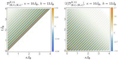
Figure 3: (Color online). Response and correlation function of the longitudinal magnetization (see (25) and (26)) far away from the critical point.

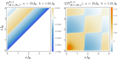
Figure 4: (Color online). Response and correlation functions of the longitudinal magnetization (see (25) and (26)) close to the critical point.

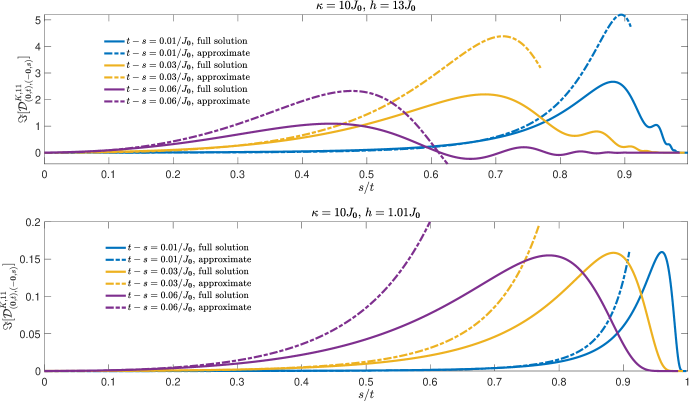
Figure 5: (Color online). Behavior of the correlation of the longitudinal magnetization as a function of the ratio of the two times, both away (upper panel) and close to (lower panel) the critical point. Different colors correspond to different values of the time difference. The dashed lines indicate the asymptotic solution at small times from (2) of the two-time correlation function.

III.1 Relaxation dynamics and aging

By inverting the operator (27) we obtain the four different response (25) and correlation (26) functions. The four components correspond to the magnetization, the current, and the two mixed correlators. In Figs. 3 and 4 we provide an example of the magnetization response and correlation functions. Fig. 3 shows results computed far away from the critical point of the closed system, which is defined by $h=J_{\mathbf{0}}$. The response function has the correct causal structure. It is also apparently translation invariant, i.e. it depends only on the time difference $t-s$. The latter is a property of our approximation which should be valid in the weakly interacting regime $\kappa\gg J$ (see discussion in Sec. II.3). Before decaying exponentially at late times, both the response and correlation functions show an oscillatory behavior with frequency $2\mathcal{R}_{\mathbf{p}}$ with $\mathcal{R}_{\mathbf{p}}=\sqrt{h\left(h-J_{\mathbf{p}}\right)}$ bounded from below by the distance $\mathcal{R}_{\mathbf{0}}$ to the critical point. When $\mathcal{R}_{\mathbf{p}}$ is small for $\mathbf{p}\to 0$ and $h\to J_{\mathbf{0}}^{+}$, as is the case in Fig. 4, the oscillations do not have time to develop before the envelope decays exponentially to zero.

The exponential decay of the correlations towards zero for late times is consistent with the expectation that the system relaxes to an infinite-temperature state due to the presence of noise.Marino and Silva (2012) However, due to the quench that leads to the breaking of time-translation invariance, two-point functions must still depend on both times $t,s$ (and not only on their difference) up to a certain equilibration time $\tau_{\rm eq}$. The latter is set in our case by the exponential decay and is proportional to the inverse noise strength: $\tau_{\rm eq}\sim 1/\kappa$. For times smaller than $1/\kappa$ we can analytically compute response and correlation functions as given in (1) and (2) for $t>s$. They explicitly depend not only on the time difference $t-s$ but also on their sum or, equivalently, on the ratio $s/t$. As long as these functions depend on $s/t$ the system has not relaxed to its equilibrium state, as is the case for systems showing aging. The dependence of the correlation function on $s/t$ is shown in Fig. 5 for different values of the time difference. After a given time the curves decay to zero and flatten out, indicating relaxation to a time-translation invariant state. On the other hand, for intermediate times there is a strong dependence on $s/t$ and the correlation function agrees well with the analytic form (2).

III.2 Critical scaling behavior

For a quench to the critical point of the noiseless system $h=J_{\mathbf{0}}$ and restricting to $0<\sigma<2$ as well distances such that $|\mathbf{p}|a\ll 1$, we have

$$J_{\mathbf{p}}/J\overset{\mathbf{p}\to\mathbf{0}}{\simeq}c_{0}-c_{\sigma}|\mathbf{p}|^{\sigma},$$ (30)

where we have chosen the lattice spacing $a$ as our unit of length and $c_{0},c_{\sigma}$ are positive pure numbers depending on the dimension $d$. In $d=1$ we have for instance $c_{0}=2\zeta(1+\sigma)$, $c_{\sigma}=-2\cos(\pi\sigma/2)\Gamma[-\sigma]$. At the critical point we have thus

$$\mathcal{R}_{\mathbf{p}}\simeq J\sqrt{c_{0}c_{\sigma}}|\mathbf{p}|^{\sigma/2}.$$ (31)

For times $t,s\ll 1/\kappa$ such that we can neglect the exponential term in (2), and for momenta such that $\kappa\gg\mathcal{R}_{\mathbf{p}}$, i.e. distances much longer than $a(J/\kappa)^{2/\sigma}$, we can approximate the response and correlation functions of (1) and (2) as

$$\langle\mathcal{M}_{\mathbf{p},t}\tilde{\mathcal{M}}_{\mathbf{p},s}\rangle\simeq-\frac{\text{i}\kappa}{4J\sqrt{c_{0}c_{\sigma}}|\mathbf{p}|^{\sigma/2}}\sin[2\sqrt{c_{0}c_{\sigma}}|\mathbf{p}|^{\sigma/2}J(t-s)],$$ (32)

$$\langle\mathcal{M}_{\mathbf{p},t}\mathcal{M}_{-\mathbf{p},s}\rangle\simeq\bigg{\{}\cos\left[2\sqrt{c_{0}c_{\sigma}}|\mathbf{p}|^{\sigma/2}J(t-s)\left(\frac{1+s/t}{1-s/t}\right)\right]$$

$$-\cos[2\sqrt{c_{0}c_{\sigma}}|\mathbf{p}|^{\sigma/2}J(t-s)]\bigg{\}}\frac{4c_{0}}{c_{\sigma}|\mathbf{p}|^{\sigma}}.$$ (33)

The above critical response and correlation functions can be brought into the scaling form given in (3) and (4), which is consistent with the scaling form expected for the model A dynamical universality classHohenberg and Halperin (1977); Calabrese and Gambassi (2005) (we recall that our Langevin equation takes the model A form (21) with no conserved quantities). We thus get the critical exponents given in (7). It is interesting to note that while the dynamical critical exponent $z$ agrees with the thermal equilibrium value, the initial-slip exponent $\theta$ deviates from the value expected for the model A class in contact with a thermal bath.Calabrese and Gambassi (2005) This feature might be interpreted as an example of a “hierarchical shell structure of nonequilibrium criticality” as proposed in Ref. Sieberer et al., 2014, whereby the dynamical universality class is further refined by an additional exponent in an open system without detailed balance. In our case the universal exponents are valid in the weakly-interacting regime $\kappa\gg J$, where the critical behavior is governed by a fixed point dominated by the noisy longitudinal field with zero average. Differently from Ref. Sieberer et al., 2014 where a driven-dissipative steady state is considered, in our case detailed balance at early times is broken by the post-quench aging behavior, whereby the additional slip exponent emerges.

IV Conclusion and outlook

We considered the long-range transverse-field Ising model with power-law interactions, where we perform a quench on the disordered side of the equilibrium phase diagram in the presence of a noisy longitudinal magnetic field with zero average. We showed that the dynamics exhibits aging at short to intermediate times before the system eventually settles into an infinite-temperature state. At these early times and at long distances we also find a scaling regime governed by a non-equilibrium fixed point dominated by the noise fluctuations. Interestingly, the universal initial-slip exponent $\theta=1$ that we find deviates from the value expected for the model A dynamical universality class in contact with a thermal bath. This suggests the emergence of a hierarchical shell structure of nonequilibrium criticality in concomitance with aging in open systems. We defer a thorough investigation of this scenario to a future work.

An important feature of the present analysis is that it puts forward a new approach for computing two-time response and correlation functions of quantum spin models undergoing dephasing. The method involves the derivation of an effective Langevin equation from which to compute two-point correlators within a self-consistent approximation. Our method can be readily extended to other quantum many-body systems with different symmetries under the influence of dephasing.

Appendix A Further details on the derivation of the Langevin equation

A.1 Effective Keldysh action

In the main text, we presented the partition function

$$\mathcal{Z}=\int\limits\mathscr{D}[\bar{\phi}^{\chi},\phi^{\chi},\lambda,\eta]\text{e}^{\text{i}\mathcal{S}[\bar{\phi}^{\chi},\phi^{\chi},\lambda,\eta]},$$

which one obtains upon averaging over the Gaussian noise, with the action given by

$$\mathcal{S}[\bar{\phi}^{\chi},\phi^{\chi},\lambda,\eta]= \int\limits_{0}^{\infty}\mathrm{d}t\sum_{\chi=\pm}\chi\big{(}\sum_{i}\bar{\phi}_{i,\alpha,t}^{\chi}\text{i}\partial_{t}\phi_{i,\alpha,t}^{\chi}-H[\bar{\phi}^{\chi},\phi^{\chi},\lambda,\eta]\big{)}+\frac{\text{i}}{\kappa}\int\limits_{0}^{\infty}\mathrm{d}t\;\sum_{i}\eta_{i,t}^{2},$$ (34)

$$H[\bar{\phi}^{\chi},\phi^{\chi},\lambda,\eta]= -\frac{1}{2}\sum_{i\neq j}J_{ij}\text{sgn}{(}\alpha)\text{sgn}{(}\beta)\bar{\phi}_{i,\alpha,t}^{\chi}\phi_{i,\alpha,t}^{\chi}\bar{\phi}_{j,\beta,t}^{\chi}\phi_{j,\beta,t}^{\chi}-h\sum_{i}\bar{\phi}_{i,\alpha,t}^{\chi}\phi_{i,\bar{\alpha},t}^{\chi}$$

$$+\sum_{i}\eta_{i,t}\text{sgn}{(}\alpha)\bar{\phi}_{i,\alpha,t}^{\chi}\phi_{i,\alpha,t}^{\chi}+\sum_{i}\lambda_{i,t}\big{(}\bar{\phi}_{i,\alpha,t}^{\chi}\phi_{i,\alpha,t}^{\chi}-2S\big{)},$$ (35)

and $\chi=\pm$ indicates dynamics along the forward (backward) branch of the contour. We now perform the Hubbard-Stratonovich (HS) transformation by inserting in (A.1) the “fat unity”

$$1=\int\limits\mathscr{D}[\mathcal{M}^{\chi}]\text{e}^{-\text{i}\int\limits_{0}^{\infty}\mathrm{d}t\;\sum_{i\neq j}\mathcal{M}_{i,t}^{\chi}\frac{\chi}{2}J_{ij}\mathcal{M}_{j,t}^{\chi}},$$ (36)

where a trivial prefactor has been absorbed into the measure. We shift the HS field $\mathcal{M}_{i,t}^{\chi}\to\mathcal{M}^{\chi}_{i,t}-\text{sgn}{(}\alpha)\bar{\phi}_{i,\alpha,t}^{\chi}\phi_{i,\alpha,t}^{\chi}$, which brings the Keldysh action in the form (17), and then perform the Keldysh rotation

$$\phi_{i,\alpha,t}^{\chi}=\frac{1}{\sqrt{2}}\left(\phi_{i,\alpha,t}^{\text{cl}}+\chi\phi_{i,\alpha,t}^{\text{q}}\right),$$ (37)

$$\mathcal{M}_{i,t}^{\chi}=\mathcal{M}^{\text{cl}}_{i,t}+\chi\mathcal{M}^{\text{q}}_{i,t},$$ (38)

where “cl” and “q” denote the classical and quantum components of the field. Note that the fields $\eta_{i,t}$ and $\lambda_{i,t}$ are classical and, therefore, have no quantum component. (37) and (38) put the action (17) in the form

$$\mathcal{S}[\bar{\phi}^{\text{cl}(\text{q})},\phi^{\text{cl}(\text{q})},\lambda,\eta,\mathcal{M}^{\text{cl}(\text{q})}]=$$

$$\int\limits_{0}^{\infty}\mathrm{d}t\int\limits_{0}^{\infty}\mathrm{d}t^{\prime}\;\sum_{i,j}\bar{\Phi}_{i,t}\left[\mathcal{G}^{-1}_{(i,t),(j,t^{\prime})}+V_{(i,t),(j,t^{\prime})}\right]\Phi_{j,t^{\prime}}$$

$$+\int\limits_{0}^{\infty}\mathrm{d}t\;\left[\frac{\text{i}}{\kappa}\sum_{i}\eta_{i,t}^{2}-\sum_{i\neq j}J_{ij}\left(\mathcal{M}^{\text{cl}}_{i,t}\mathcal{M}^{\text{q}}_{j,t}+\mathcal{M}^{\text{q}}_{i,t}\mathcal{M}^{\text{cl}}_{j,t}\right)\right],$$ (39)

where $\Phi_{i,t}=(\phi_{i,\uparrow,t}^{\text{cl}},\phi_{i,\downarrow,t}^{\text{cl}},\phi_{i,\uparrow,t}^{\text{q}},\phi_{i,\downarrow,t}^{\text{q}})^{\intercal}$, and we have split the bosonic-field part of the action into a free term described by

$$\mathcal{G}_{(i,t),(j,t^{\prime})}^{-1}=\begin{pmatrix}0&\left[\mathcal{G}_{(i,t),(j,t^{\prime})}^{-1}\right]^{\text{A}}\\ \left[\mathcal{G}_{(i,t),(j,t^{\prime})}^{-1}\right]^{\text{R}}&\left[\mathcal{G}_{(i,t),(j,t^{\prime})}^{-1}\right]^{\text{K}}\end{pmatrix},$$ (40)

$$\left[\mathcal{G}_{(i,t),(j,t^{\prime})}^{-1}\right]^{\text{R}(\text{A})}=\;\delta_{i,j}\delta(t-t^{\prime})\left[(\text{i}\partial_{t}\pm\text{i}\varepsilon)\sigma^{0}+h\sigma^{x}\right],$$ (41)

$$\left[\mathcal{G}_{(i,t),(j,t^{\prime})}^{-1}\right]^{\text{K}}=\;2\text{i}\varepsilon\begin{pmatrix}F^{\uparrow\uparrow}(t,t^{\prime})&F^{\uparrow\downarrow}(t,t^{\prime})\\ F^{\downarrow\uparrow}(t,t^{\prime})&F^{\downarrow\downarrow}(t,t^{\prime})\end{pmatrix}\delta_{i,j},$$ (42)

where (42) serves as a pure regularization term that is necessary for $\mathcal{G}^{-1}$ to be invertible with $\varepsilon\to 0$ and $F^{\alpha\beta}(t,t^{\prime})$ are (upon Wigner transformation) distribution functions, and into a “source” term described by

$$V_{(i,t),(j,t^{\prime})}=\begin{pmatrix}V_{(i,t),(j,t^{\prime})}^{\text{q}}&V_{(i,t),(j,t^{\prime})}^{\text{cl}}\\ V_{(i,t),(j,t^{\prime})}^{\text{cl}}&V_{(i,t),(j,t^{\prime})}^{\text{q}}\end{pmatrix},$$ (43)

$$V_{(i,t),(j,t^{\prime})}^{\text{q}}=\;\sum_{l}J_{il}\mathcal{M}^{\text{q}}_{l,t}\sigma^{z}\delta_{i,j}\delta(t-t^{\prime}),$$ (44)

$$V_{(i,t),(j,t^{\prime})}^{\text{cl}}=\;\delta_{i,j}\delta(t-t^{\prime})\bigg{[}\big{(}\sum_{l}J_{il}\mathcal{M}^{\text{cl}}_{l,t}-\eta_{i,t}\big{)}\sigma^{z}-\lambda_{i,t}\sigma^{0}\bigg{]}.$$ (45)

Inverting (41) yields the free retarded and advanced propagators

$$\mathcal{G}_{(i,t),(j,t^{\prime})}^{\text{R}(\text{A}),\uparrow\uparrow} =\mp\text{i}\text{e}^{\mp\varepsilon(t-t^{\prime})}\Theta[\pm(t-t^{\prime})]\cos[h(t-t^{\prime})],$$ (46)

$$\mathcal{G}_{(i,t),(j,t^{\prime})}^{\text{R}(\text{A}),\uparrow\downarrow} =\pm\text{e}^{\mp\varepsilon(t-t^{\prime})}\Theta[\pm(t-t^{\prime})]\sin[h(t-t^{\prime})],$$ (47)

and where due to $\mathbb{Z}_{2}$ symmetry we have $\mathcal{G}_{(i,t),(j,t^{\prime})}^{\text{R}(\text{A}),\uparrow\uparrow}=\mathcal{G}_{(i,t),(j,t^{\prime})}^{\text{R}(\text{A},),\downarrow\downarrow}$ and $\mathcal{G}_{(i,t),(j,t^{\prime})}^{\text{R}(\text{A}),\uparrow\downarrow}=\mathcal{G}_{(i,t),(j,t^{\prime})}^{\text{R}(\text{A},),\downarrow\uparrow}$. Integrating out the bosonic degrees of freedom in the partition function

$$\mathcal{Z}= \int\limits\mathscr{D}[\bar{\phi}^{\text{cl}(\text{q})},\phi^{\text{cl}(\text{q})},\lambda,\eta,\mathcal{M}^{\text{cl}(\text{q})}]\text{e}^{\text{i}\mathcal{S}[\bar{\phi}^{\text{cl}(\text{q})},\phi^{\text{cl}(\text{q})},\lambda,\eta,\mathcal{M}^{\text{cl}(\text{q})}]}$$

$$= \int\limits\mathscr{D}[\lambda,\eta,\mathcal{M}^{\text{cl}(\text{q})}]\text{e}^{\text{i}\mathcal{S}_{\text{eff}}[\lambda,\eta,\mathcal{M}^{\text{cl}(\text{q})}]},$$ (48)

leads to the effective Keldysh action

$$\mathcal{S}_{\text{eff}}[\lambda,\eta,\mathcal{M},\tilde{\mathcal{M}}]=\text{i}\operatorname{Tr}\ln\mathcal{G}^{-1}+\text{i}\operatorname{Tr}\ln\left(1+\mathcal{G}V\right)$$

$$+\int\limits_{0}^{\infty}\mathrm{d}t\;\left[\frac{\text{i}}{\kappa}\sum_{i}\eta_{i,t}^{2}-\sum_{i\neq j}J_{ij}\left(\mathcal{M}^{\text{cl}}_{i,t}\mathcal{M}^{\text{q}}_{j,t}+\mathcal{M}^{\text{q}}_{i,t}\mathcal{M}^{\text{cl}}_{j,t}\right)\right].$$ (49)

$1+\mathcal{G}V$ is not diagonal in Keldysh, Nambu, or time space. We therefore Taylor-expand its inverse $(1+\mathcal{G}V)^{-1}$, which up to second order in $V$ leads to the saddle-point solution

$$\mathcal{M}_{i,t}=-2\text{i}\int\limits_{0}^{\infty}\mathrm{d}\tau\Big{(}\sum_{l}J_{il}\mathcal{M}_{l,\tau}-\eta_{i,\tau}\Big{)}\times$$

$$\times\Big{(}\Re\mathcal{G}_{(i,\tau),(i,t)}^{\text{K},\uparrow\uparrow}\mathcal{G}_{(i,t),(i,\tau)}^{\text{R},\uparrow\uparrow}-\text{i}\Im\mathcal{G}_{(i,\tau),(i,t)}^{\text{K},\uparrow\downarrow}\mathcal{G}_{(i,t),(i,\tau)}^{\text{R},\downarrow\uparrow}\Big{)},$$ (50)

and this entails setting $\mathcal{M}^{\text{q}}\to 0$, and we have thus dropped the superscript “cl” from the classical magnetization field $\mathcal{M}_{i,t}\equiv\mathcal{M}^{\text{cl}}_{i,t}$ for notational brevity.

A.2 Self-energies

In order for $\mathcal{M}_{i,t}$ to be self-consistent, we must now calculate the self-energies. This is conveniently achieved by calculating the full propagator

$$G^{uw}_{(l,\gamma,\tau),(m,\mu,\tau^{\prime})}= -\text{i}\langle\phi_{l,\gamma,\tau}^{u}\bar{\phi}_{m,\mu,\tau^{\prime}}^{w}\rangle$$

$$= -\text{i}\langle\phi_{l,\gamma,\tau}^{u}\bar{\phi}_{m,\mu,\tau^{\prime}}^{w}\text{e}^{\text{i}\mathcal{S}_{V}}\rangle_{0},$$ (51)

by expanding up to second order in the interaction part of the action (39)

$$\mathcal{S}_{V}[\bar{\phi},\phi,\lambda,\eta,\mathcal{M},\mathcal{M}^{\text{q}}]= \int\limits_{0}^{\infty}\mathrm{d}t\int\limits_{0}^{\infty}\mathrm{d}t^{\prime}\;\sum_{i,j}\bar{\Phi}_{i,t}V_{(i,t),(j,t^{\prime})}\Phi_{j,t^{\prime}}.$$ (52)

The self-energies arising from this expansion by approximating the Dyson equation as

$$G=\mathcal{G}+\mathcal{G}\Sigma G\approx\mathcal{G}+\mathcal{G}\Sigma\mathcal{G},$$ (53)

are

$$\Sigma^{\text{R},\text{A},\text{K}}_{(i,t),(j,t^{\prime})}= \frac{\kappa}{2}\delta_{i,j}\delta(t-t^{\prime})\sigma^{0}$$

$$+\sum_{l,r}J_{il}J_{jr}\langle\mathcal{M}_{l,t}\mathcal{M}_{r,t^{\prime}}\rangle_{0}\sigma^{z}\mathcal{G}^{\text{R},\text{A},\text{K}}_{(i,t),(j,t^{\prime})}\sigma^{z},$$ (54)

where, as mentioned previously, we take $\mathcal{M}^{\text{q}}\to 0$. Recasting the Dyson equation in the form

$$\mathds{1}_{4\times 4} =\begin{pmatrix}0&\left[\mathcal{G}^{-1}\right]^{\text{A}}-\Sigma^{\text{A}}\\ \left[\mathcal{G}^{-1}\right]^{\text{R}}-\Sigma^{\text{R}}&-\Sigma^{\text{K}}\end{pmatrix}\begin{pmatrix}G^{\text{K}}&G^{\text{R}}\\ G^{\text{A}}&0\end{pmatrix},$$ (55)

and taking $J\ll\kappa$ while considering the dynamics to always be restricted to the disordered phase, the retarded and advanced full propagators can then be calculated to be (19) in the main text.

Also from (55), upon enforcing self-consistency through replacing $\mathcal{G}^{\text{K}}$ with $G^{\text{K}}$ in the expression for $\Sigma^{\text{K}}$ (which for clarity we shall now call $\tilde{\Sigma}^{\text{K}}$) we obtain

$$\Big{(}\left[\mathcal{G}^{-1}\right]^{\text{R}}-\Sigma^{\text{R}}\Big{)}G^{\text{K}}=\tilde{\Sigma}^{\text{K}}G^{\text{A}},$$ (56)

from which we calculate the Keldysh full propagator (20) presented in the main text. Replacing $\mathcal{G}^{\text{K}(\text{R})}$ with $G^{\text{K}(\text{R})}$ in (50), we arrive at (18) in the main text. Fourier-transforming from position into momentum space, and thereafter carrying out a time derivative twice, we arrive at the second-order differential equation

$$\left(\partial^{2}_{t}+\kappa\partial_{t}+4h^{2}+\frac{\kappa^{2}}{4}-4hJ_{\mathbf{p}}\text{e}^{-\kappa t}\right)\mathcal{M}_{\mathbf{p},t}$$

$$=-4h\text{e}^{-\kappa t}\eta_{\mathbf{p},t},$$ (57)

which is then transformed into a first-order Langevin vector equation (21) as illustrated in the main text.

References

- Cardy (1996) J. Cardy, Scaling and Renormalization in Statistical Physics, Cambridge Lecture Notes in Physics (Cambridge University Press, 1996), ISBN 9780521499590, URL https://books.google.de/books?id=Wt804S9FjyAC.
- Sachdev (2001) S. Sachdev, Quantum Phase Transitions (Cambridge University Press, 2001), ISBN 9780521004541, URL https://books.google.de/books?id=Ih_E05N5TZQC.
- Ma (1985) S. Ma, Statistical Mechanics (World Scientific, 1985), ISBN 9789971966065, URL https://books.google.de/books?id=YW-0AQAACAAJ.
- Wilson (1971a) K. G. Wilson, Phys. Rev. B 4, 3174 (1971a), URL https://link.aps.org/doi/10.1103/PhysRevB.4.3174.
- Wilson (1971b) K. G. Wilson, Phys. Rev. B 4, 3184 (1971b), URL https://link.aps.org/doi/10.1103/PhysRevB.4.3184.
- Wilson and Fisher (1972) K. G. Wilson and M. E. Fisher, Phys. Rev. Lett. 28, 240 (1972), URL https://link.aps.org/doi/10.1103/PhysRevLett.28.240.
- Wilson and Kogut (1974) K. G. Wilson and J. Kogut, Physics Reports 12, 75 (1974), ISSN 0370-1573, URL http://www.sciencedirect.com/science/article/pii/0370157374900234.
- Fisher (1974) M. E. Fisher, Rev. Mod. Phys. 46, 597 (1974), URL https://link.aps.org/doi/10.1103/RevModPhys.46.597.
- Wilson (1975) K. G. Wilson, Rev. Mod. Phys. 47, 773 (1975), URL https://link.aps.org/doi/10.1103/RevModPhys.47.773.
- Porras and Cirac (2004) D. Porras and J. I. Cirac, Phys. Rev. Lett. 92, 207901 (2004), URL https://link.aps.org/doi/10.1103/PhysRevLett.92.207901.
- Kim et al. (2009) K. Kim, M.-S. Chang, R. Islam, S. Korenblit, L.-M. Duan, and C. Monroe, Phys. Rev. Lett. 103, 120502 (2009), URL https://link.aps.org/doi/10.1103/PhysRevLett.103.120502.
- Jurcevic et al. (2014) P. Jurcevic, B. P. Lanyon, P. Hauke, C. Hempel, P. Zoller, R. Blatt, and C. F. Roos, Nature 511, 202–205 (2014), URL http://www.nature.com/articles/nature13461.
- Levin et al. (2012) K. Levin, A. Fetter, and D. Stamper-Kurn, Ultracold Bosonic and Fermionic Gases, Contemporary Concepts of Condensed Matter Science (Elsevier Science, 2012), ISBN 9780444538628, URL https://books.google.de/books?id=rLlplpMuX6oC.
- Yukalov (2011) V. I. Yukalov, Laser Physics Letters 8, 485 (2011), URL http://stacks.iop.org/1612-202X/8/i=7/a=001.
- Bloch et al. (2008) I. Bloch, J. Dalibard, and W. Zwerger, Rev. Mod. Phys. 80, 885 (2008), URL https://link.aps.org/doi/10.1103/RevModPhys.80.885.
- Greiner et al. (2002) M. Greiner, O. Mandel, T. W. Hänsch, and I. Bloch, Nature 419, 51–54 (2002), URL https://www.nature.com/articles/nature00968.
- Täuber (2014) U. Täuber, Critical Dynamics: A Field Theory Approach to Equilibrium and Non-Equilibrium Scaling Behavior (Cambridge University Press, 2014), ISBN 9780521842235, URL https://books.google.de/books?id=qtTSAgAAQBAJ.
- Zvyagin (2016) A. A. Zvyagin, Low Temperature Physics 42, 971 (2016), URL https://aip.scitation.org/doi/10.1063/1.4969869.
- Heyl (2018) M. Heyl, Reports on Progress in Physics 81, 054001 (2018), URL http://stacks.iop.org/0034-4885/81/i=5/a=054001.
- Mori et al. (2017) T. Mori, T. N. Ikeda, E. Kaminishi, and M. Ueda, ArXiv e-prints (2017), eprint 1712.08790, URL https://arxiv.org/abs/1712.08790.
- Nicklas et al. (2015) E. Nicklas, M. Karl, M. Höfer, A. Johnson, W. Muessel, H. Strobel, J. Tomkovič, T. Gasenzer, and M. K. Oberthaler, Phys. Rev. Lett. 115, 245301 (2015), URL https://link.aps.org/doi/10.1103/PhysRevLett.115.245301.
- Zhang et al. (2017) J. Zhang, G. Pagano, P. W. Hess, A. Kyprianidis, P. Becker, H. Kaplan, A. V. Gorshkov, Z.-X. Gong, and C. Monroe, Nature 551, 601 (2017), URL https://www.nature.com/articles/nature24654.
- Jurcevic et al. (2017) P. Jurcevic, H. Shen, P. Hauke, C. Maier, T. Brydges, C. Hempel, B. P. Lanyon, M. Heyl, R. Blatt, and C. F. Roos, Phys. Rev. Lett. 119, 080501 (2017), URL https://link.aps.org/doi/10.1103/PhysRevLett.119.080501.
- Neyenhuis et al. (2017) B. Neyenhuis, J. Zhang, P. W. Hess, J. Smith, A. C. Lee, P. Richerme, Z.-X. Gong, A. V. Gorshkov, and C. Monroe, Science Advances 3 (2017), URL http://advances.sciencemag.org/content/3/8/e1700672.
- Fläschner et al. (2018) N. Fläschner, D. Vogel, M. Tarnowski, B. S. Rem, D.-S. Lühmann, M. Heyl, J. C. Budich, L. Mathey, K. Sengstock, and C. Weitenberg, Nature Physics 14, 265 (2018), ISSN 1745-2481, URL https://doi.org/10.1038/s41567-017-0013-8.
- Hohenberg and Halperin (1977) P. C. Hohenberg and B. I. Halperin, Reviews of Modern Physics 49, 435 (1977).
- Berges et al. (2004) J. Berges, S. Borsányi, and C. Wetterich, Phys. Rev. Lett. 93, 142002 (2004), URL http://link.aps.org/doi/10.1103/PhysRevLett.93.142002.
- Kitagawa et al. (2011) T. Kitagawa, A. Imambekov, J. Schmiedmayer, and E. Demler, New Journal of Physics 13, 073018 (2011), URL http://stacks.iop.org/1367-2630/13/i=7/a=073018.
- Gring et al. (2012) M. Gring, M. Kuhnert, T. Langen, T. Kitagawa, B. Rauer, M. Schreitl, I. Mazets, D. A. Smith, E. Demler, and J. Schmiedmayer, Science 337, 1318 (2012).
- Langen et al. (2013) T. Langen, R. Geiger, M. Kuhnert, B. Rauer, and J. Schmiedmayer, Nat Phys 9, 640 (2013), URL http://dx.doi.org/10.1038/nphys2739.
- van den Worm et al. (2013) M. van den Worm, B. C. Sawyer, J. J. Bollinger, and M. Kastner, New Journal of Physics 15, 083007 (2013), URL http://stacks.iop.org/1367-2630/15/i=8/a=083007.
- Marcuzzi et al. (2013) M. Marcuzzi, J. Marino, A. Gambassi, and A. Silva, Phys. Rev. Lett. 111, 197203 (2013), URL http://link.aps.org/doi/10.1103/PhysRevLett.111.197203.
- Chiocchetta et al. (2015) A. Chiocchetta, M. Tavora, A. Gambassi, and A. Mitra, Phys. Rev. B 91, 220302 (2015), URL http://link.aps.org/doi/10.1103/PhysRevB.91.220302.
- Chiocchetta et al. (2017) A. Chiocchetta, A. Gambassi, S. Diehl, and J. Marino, Phys. Rev. Lett. 118, 135701 (2017), URL https://link.aps.org/doi/10.1103/PhysRevLett.118.135701.
- Maraga et al. (2015) A. Maraga, A. Chiocchetta, A. Mitra, and A. Gambassi, Phys. Rev. E 92, 042151 (2015), URL https://link.aps.org/doi/10.1103/PhysRevE.92.042151.
- Sciolla and Biroli (2013) B. Sciolla and G. Biroli, Phys. Rev. B 88, 201110 (2013), URL http://link.aps.org/doi/10.1103/PhysRevB.88.201110.
- Sciolla and Biroli (2010) B. Sciolla and G. Biroli, Phys. Rev. Lett. 105, 220401 (2010), URL https://link.aps.org/doi/10.1103/PhysRevLett.105.220401.
- Sciolla and Biroli (2011) B. Sciolla and G. Biroli, Journal of Statistical Mechanics: Theory and Experiment 2011, P11003 (2011), URL http://stacks.iop.org/1742-5468/2011/i=11/a=P11003.
- Homrighausen et al. (2017) I. Homrighausen, N. O. Abeling, V. Zauner-Stauber, and J. C. Halimeh, Phys. Rev. B 96, 104436 (2017), URL https://link.aps.org/doi/10.1103/PhysRevB.96.104436.
- Lang et al. (2018) J. Lang, B. Frank, and J. C. Halimeh, Phys. Rev. B 97, 174401 (2018), URL https://link.aps.org/doi/10.1103/PhysRevB.97.174401.
- Calabrese and Gambassi (2005) P. Calabrese and A. Gambassi, Journal of Physics A: Mathematical and General 38, R133 (2005), URL http://stacks.iop.org/0305-4470/38/i=18/a=R01.
- Janssen et al. (1989) H. K. Janssen, B. Schaub, and B. Schmittmann, Zeitschrift für Physik B Condensed Matter 73, 539 (1989), ISSN 1431-584X, URL https://doi.org/10.1007/BF01319383.
- Gambassi and Calabrese (2011) A. Gambassi and P. Calabrese, EPL (Europhysics Letters) 95, 66007 (2011), URL http://stacks.iop.org/0295-5075/95/i=6/a=66007.
- Sieberer et al. (2013) L. M. Sieberer, S. D. Huber, E. Altman, and S. Diehl, Phys. Rev. Lett. 110, 195301 (2013), URL http://link.aps.org/doi/10.1103/PhysRevLett.110.195301.
- Gagel et al. (2014) P. Gagel, P. P. Orth, and J. Schmalian, Phys. Rev. Lett. 113, 220401 (2014), URL http://link.aps.org/doi/10.1103/PhysRevLett.113.220401.
- Lang and Piazza (2016) J. Lang and F. Piazza, Phys. Rev. A 94, 033628 (2016), URL https://link.aps.org/doi/10.1103/PhysRevA.94.033628.
- Marino and Silva (2012) J. Marino and A. Silva, Phys. Rev. B 86, 060408 (2012), URL http://link.aps.org/doi/10.1103/PhysRevB.86.060408.
- Sciolla et al. (2015) B. Sciolla, D. Poletti, and C. Kollath, Phys. Rev. Lett. 114, 170401 (2015), URL http://link.aps.org/doi/10.1103/PhysRevLett.114.170401.
- Lorenzo et al. (2017) S. Lorenzo, T. Apollaro, G. Palma, R. Nandkishore, A. Silva, and J. Marino, arXiv preprint arXiv:1712.05793 (2017).
- Maghrebi et al. (2016) M. F. Maghrebi, Z.-X. Gong, M. Foss-Feig, and A. V. Gorshkov, Physical Review B 93, 125128 (2016).
- Kamenev (2011) A. Kamenev, Field Theory of Non-Equilibrium Systems (Cambridge University Press, 2011), ISBN 9781139500296, URL http://books.google.de/books?id=CwlrUepnla4C.
- Danielewicz (1984) P. Danielewicz, Annals of Physics 152, 239 (1984).
- Sieberer et al. (2014) L. M. Sieberer, S. D. Huber, E. Altman, and S. Diehl, Phys. Rev. B 89, 134310 (2014), URL https://link.aps.org/doi/10.1103/PhysRevB.89.134310.