Measuring and engineering the atomic mass density wave
of a Gaussian mass-polariton pulse in optical fibers

Abstract

Conventional theories of electromagnetic waves in a medium assume that only the energy of the field propagates inside the medium. Consequently, they neglect the transport of mass density by the medium atoms. We have recently presented foundations of a covariant theory of light propagation in a nondispersive medium by considering a light wave simultaneously with the dynamics of the medium atoms driven by optoelastic forces [Phys. Rev. A 95, 063850 (2017)]. In particular, we have shown that the mass is transferred by an atomic mass density wave (MDW), which gives rise to mass-polariton (MP) quasiparticles, i.e., covariant coupled states of the field and matter having a nonzero rest mass. Another key observation of the mass-polariton theory of light is that, in common semiconductors, most of the momentum of light is transferred by moving atoms, e.g., 92% in the case of silicon. In this work, we generalize the MP theory of light for dispersive media and consider experimental measurement of the mass transferred by the MDW atoms when an intense light pulse propagates in a silicon fiber. In particular, we consider optimal intensity and time dependence of a Gaussian pulse and account for the breakdown threshold irradiance of the material. The optical shock wave property of the MDW, which propagates with the velocity of light instead of the velocity of sound, prompts for engineering of novel device concepts like very high frequency mechanical oscillators not limited by the acoustic cutoff frequency.

1 Introduction

It is well known in the electrodynamics of continuous media that a light pulse exerts optical forces on the atoms when it propagates inside a medium [1]. However, the coupled dynamics of the field and the medium driven by the optical force density has been a subject of very few detailed studies. We have recently elaborated how the optical force density gives rise to a mass density wave (MDW) in a nondispersive medium when a light pulse is propagating in it [2]. We have also generalized the theory for dispersive media [3]. Our investigations are performed using two complementary approaches: (1) the mass-polariton (MP) quasiparticle theory, which is based on the conservation laws and the Lorentz transformation; (2) the classical optoelastic continuum dynamics (OCD), which generalizes the electrodynamics of continuous media to include the dynamics of the medium resulting from the optical force density.

The complementary MP and OCD models transparently resolve the centenary Abraham-Minkowski controversy of the momentum of light in a medium [4, 5, 6, 7, 8, 9, 10, 11, 12, 13, 14], which has also gained much experimental interest [15, 16, 17, 18, 19, 20, 21, 22, 23, 24, 25, 26]. This controversy originates from the formulation of two rivaling momentum densities for light by Abraham, $\mathbf{g}_{\mathrm{A}}=\mathbf{E}\times\mathbf{H}/c^{2}$ [27, 28], and by Minkowski, $\mathbf{g}_{\mathrm{M}}=\mathbf{D}\times\mathbf{B}$ [29], where $\mathbf{E}$ and $\mathbf{H}$ are the electric- and magnetic-field strengths, $\mathbf{D}$ and $\mathbf{B}$ are the electric and magnetic flux densities, and $c$ is the speed of light in vacuum. In contrast, in the MP theory of light, the total momentum density of light in the medium is given by $\mathbf{g}_{\mathrm{MP}}=\rho_{\mathrm{a}}\mathbf{v}_{\mathrm{a}}+\mathbf{E}\times\mathbf{H}/c^{2}$, where $\rho_{\mathrm{a}}\mathbf{v}_{\mathrm{a}}$ is the classical momentum density of the MDW atoms. For a monochromatic field, the momentum densities $\mathbf{g}_{\mathrm{A}}$, $\mathbf{g}_{\mathrm{M}}$, and $\mathbf{g}_{\mathrm{MP}}$ correspond to the single-photon momenta $p_{\mathrm{A}}=\hbar\omega/(n_{\mathrm{g}}c)$, $p_{\mathrm{M}}=n_{\mathrm{p}}^{2}\hbar\omega/(n_{\mathrm{g}}c)$, and $p_{\mathrm{MP}}=n_{\mathrm{p}}\hbar\omega/c$, respectively, where $\hbar$ is the reduced Planck constant, $\omega$ is the angular frequency of the field, and $n_{\mathrm{p}}$ and $n_{\mathrm{g}}$ are the phase and group refractive indices of the medium.

In this work, we review the foundations of the MP theory of light represented in Refs. [2, 3, 30, 31], especially concentrating in the OCD model and the generalization of the theory for dispersive media. We also consider experimental measurement of the mass transferred by the MDW atoms when an intense light pulse propagates in a silicon fiber. In particular, we study optimal intensity and time dependence of a Gaussian pulse and account for the breakdown threshold irradiance of the material.

2 Fields and the dispersion relation

In dispersive media, the phase refractive index $n_{\mathrm{p}}(\omega)$ depends on frequency. Its general relation to the wave number $k$ and frequency $\omega(k)$ is given by $\omega(k)=ck/n_{\mathrm{p}}(\omega)$, which can be used to write the phase velocity of light in a medium as $v_{\mathrm{p}}(\omega)=c/n_{\mathrm{p}}(\omega)=\omega(k)/k$. The phase velocity describes the propagation velocity of individual frequency components. Another velocity that characterizes the propagation of light in dispersive media is provided by the group velocity $v_{\mathrm{g}}(\omega)=c/n_{\mathrm{g}}(\omega)=\partial\omega(k)/\partial k$, where $n_{\mathrm{g}}(\omega)$ is the group refractive index. The group velocity describes the amplitudes of individual frequency components together produce a wave packet.

As exact solutions of Maxwell’s equations, the electric and magnetic fields of a one-dimensional light pulse that is linearly polarized along the $y$ axis and propagates in $x$ direction in a dispersive medium are written as [32]

$$\mathbf{E}(\mathbf{r},t)=\mathrm{Re}\Big{[}\int_{-\infty}^{\infty}\tilde{E}(k)e^{i[kx-\omega(k)t]}dk\Big{]}\hat{\mathbf{y}},$$ (1)

$$\mathbf{H}(\mathbf{r},t)=\mathrm{Re}\Big{[}\int_{-\infty}^{\infty}\tilde{H}(k)e^{i[kx-\omega(k)t]}dk\Big{]}\hat{\mathbf{z}}.$$ (2)

Here $\tilde{E}(k)$ and $\tilde{H}(k)$ are the Fourier components of the electric and magnetic fields, and $\hat{\mathbf{y}}$ and $\hat{\mathbf{z}}$ are unit vectors with respect to $y$ and $z$ axes, respectively. The Fourier components of the fields are related to each other by $\tilde{H}(k)=\sqrt{\varepsilon[\omega(k)]/\mu[\omega(k)]}\tilde{E}(k)$, where $\varepsilon(\omega)$ and $\mu(\omega)$ are the permittivity and permeability of the medium, which are frequency dependent in dispersive media. The permittivity and permeability are related to the phase refractive index of the medium by $\varepsilon(\omega)\mu(\omega)=\varepsilon_{0}\mu_{0}n_{\mathrm{p}}(\omega)^{2}$, in which $\varepsilon_{0}$ and $\mu_{0}$ are the permittivity and permeability of the vacuum, respectively.

In this work, we concentrate on the propagation of light pulses in the special case of linearly dispersive media. Linear dispersion is a good approximation for light pulses with the central frequency $\omega_{0}$ in any dispersive media if the spectral width $\Delta\omega/\omega_{0}$ of the wave packet is relatively small, the dispersion relation does not have resonances near $\omega_{0}$, and if the distance traveled by the wave packet is not very long. The linear dispersion relation near the central frequency $\omega_{0}$ can be written as

$$\omega(k)=\omega_{0}+(c/n_{\mathrm{g}})(k-k_{\mathrm{0,med}}),$$ (3)

where $k_{\mathrm{0,med}}=n_{\mathrm{p}}k_{0}$ is the central wave number in the medium, in which $k_{0}=\omega_{0}/c$ is the central wave number in vacuum and $n_{\mathrm{p}}=n_{\mathrm{p}}(\omega_{0})$ is the phase refractive index for $\omega_{0}$, and the group refractive index $n_{\mathrm{g}}$ is constant. The special feature of the linear form of the dispersion relation in Eq. (3) is that it does not lead to the distortion of the pulse envelope while the pulse propagates. For frequencies deviating from $\omega_{0}$, the linear dispersion relation in Eq. (3) defines the frequency-dependent phase refractive index as $n_{\mathrm{p}}(\omega)=n_{\mathrm{g}}+(n_{\mathrm{p}}-n_{\mathrm{g}})\omega_{0}/\omega$.

In this work, we make simulations using Gaussian light pulses with $\tilde{E}(k)=\tilde{E}_{0}e^{-[(k-n_{\mathrm{p}}k_{0})/(n_{\mathrm{p}}\Delta k_{0})]^{2}/2}$, where $\tilde{E}_{0}$ is a normalization factor and $\Delta k_{0}$ is the standard deviation of the wave number in vacuum, which determines the pulse width in the $x$ direction as $\Delta x=1/(\sqrt{2}n_{\mathrm{p}}\Delta k_{0})$. The standard deviation of the pulse width in time is given by $\Delta t=n_{\mathrm{p}}\Delta x/c=1/(\sqrt{2}\Delta k_{0}c)$ and the corresponding full width at half maximum (FWHM) is $\Delta t_{\mathrm{FWHM}}=2\sqrt{2\ln 2}\,\Delta t$. Applying the linear dispersion relation in Eq. (3) with the expression of the electric field in Eq. (1), the integration with respect to $k$ can be performed analytically and the electric field becomes

$$\mathbf{E}(\mathbf{r},t)=\sqrt{2\pi}\,n_{\mathrm{p}}\Delta k_{0}\tilde{E}_{0}\cos\Big{[}n_{\mathrm{p}}k_{0}\Big{(}x-\frac{ct}{n_{\mathrm{p}}}\Big{)}\Big{]}e^{-(n_{\mathrm{p}}\Delta k_{0})^{2}(x-ct/n_{\mathrm{g}})^{2}/2}\hat{\mathbf{y}}.$$ (4)

In the simulations, we determine the normalization factor $\tilde{E}_{0}$ in Eq. (4) so that the integral of the corresponding instantaneous energy density over $x$ gives $U_{0}/A$, where $U_{0}$ is the total electromagnetic energy of the light pulse and $A$ is the cross-sectional area.

3 Optoelastic continuum dynamics

3.1 Newton’s equation of motion and optoelastic forces

In the OCD model, a light pulse is optoelastically coupled to the medium through the optical force density, which gives rise to an atomic MDW in the medium. Due to the MDW effect, the mass density of the medium $\rho_{\mathrm{a}}$ is perturbed from its equilibrium value $\rho_{0}$. For a light pulse propagating in a homogeneous medium, the perturbed mass density can be written as $\rho_{\mathrm{a}}(\mathbf{r},t)=\rho_{0}+\rho_{\text{\tiny MDW}}(\mathbf{r},t)$, where $\rho_{\text{\tiny MDW}}(\mathbf{r},t)$ is the mass density of the MDW. As the atomic velocities are nonrelativistic, we can write Newton’s equation of motion for the mass density of the medium $\rho_{\mathrm{a}}(\mathbf{r},t)$ as [2]

$$\rho_{\mathrm{a}}(\mathbf{r},t)\frac{d^{2}\mathbf{r}_{\mathrm{a}}(\mathbf{r},t)}{dt^{2}}=\mathbf{f}_{\mathrm{opt}}(\mathbf{r},t)+\mathbf{f}_{\mathrm{el}}(\mathbf{r},t).$$ (5)

Here $\mathbf{r}_{\mathrm{a}}(\mathbf{r},t)$ is the atomic displacement field of the medium, $\mathbf{f}_{\mathrm{opt}}(\mathbf{r},t)$ is the optical force density that will be discussed in more detail below, and $\mathbf{f}_{\mathrm{el}}(\mathbf{r},t)$ is the elastic force density that acts between atoms as they are displaced from their initial equilibrium positions by the optical force density. The elastic force density for anisotropic cubic crystals, such as silicon, is given, e.g., in Ref. [33].

The correct form of the optical force density acting on the medium under the influence of time-dependent electromagnetic field has been extensively discussed in previous literature as a part of the Abraham-Minkowski controversy [34]. In the case of a nondispersive medium, we have recently shown that there is only one form of optical force density that is fully consistent with the MP quasiparticle model and the underlying principles of the special theory of relativity [2]. In this work, we generalize this optical force for dispersive dielectric media by writing

$$\mathbf{f}_{\mathrm{opt}}(\mathbf{r},t)=-\varepsilon_{0}n_{\mathrm{g}}\mathbf{E}^{2}\nabla n_{\mathrm{p}}+\frac{n_{\mathrm{p}}n_{\mathrm{g}}-1}{c^{2}}\frac{\partial}{\partial t}\mathbf{E}\times\mathbf{H},$$ (6)

where $\mathbf{E}\times\mathbf{H}=\mathbf{S}$ is the instantaneous Poynting vector. This expression of the optical force density can be justified by showing that it is the only form of the optical force density that enables covariant description of the light pulse in a dispersive medium. In calculating the optoelastic force field by using Eq. (6), we apply a perturbative approach in which the damping of the electromagnetic field due to the transfer of the field energy to the kinetic and elastic energies of atoms by the optical force is neglected. The accuracy of this approximation is estimated in the case of nondispersive media in Ref. [2]. The conclusions are also valid for lossless dispersive media where the direct optical absorption related, e.g., to the electronic excitation of the medium, is negligible.

3.2 Transferred mass and momentum of the mass density wave

The optical and elastic force densities and Newton’s equation of motion in Eq. (5) can be used to simulate the motion of atoms in the medium as a function of space and time. The total displacement of atoms at position $\mathbf{r}$ is solved from Eq. (5) by integration as

$$\mathbf{r}_{\mathrm{a}}(\mathbf{r},t)=\int_{-\infty}^{t}\int_{-\infty}^{t^{\prime\prime}}\frac{d^{2}\boldsymbol{r}_{\mathrm{a}}(\mathbf{r},t^{\prime})}{dt^{\prime 2}}dt^{\prime}dt^{\prime\prime}=\int_{-\infty}^{t}\int_{-\infty}^{t^{\prime\prime}}\frac{\mathbf{f}_{\mathrm{opt}}(\mathbf{r},t^{\prime})+\mathbf{f}_{\mathrm{el}}(\mathbf{r},t^{\prime})}{\rho_{\mathrm{a}}(\mathbf{r},t^{\prime})}dt^{\prime}dt^{\prime\prime}.$$ (7)

The perturbed mass density of the medium $\rho_{\mathrm{a}}(\mathbf{r},t)$ is extremely close to the equilibrium mass density $\rho_{0}$ as the total mass of atoms inside the light pulse is very large compared to mass equivalent of the field energy. Therefore, the mass density in the denominator of the integrand in Eq. (7) can be approximated with the equilibrium mass density $\rho_{0}$.

When the light pulse has passed the position $\mathbf{r}$ at the instance of time $t_{\mathrm{pass}}$, the displacement of atoms at $\mathbf{r}$ is given by $\mathbf{r}_{\mathrm{a}}(\mathbf{r},t_{\mathrm{pass}})$. One can then obtain the total displaced volume as $\delta V=\int\mathbf{r}_{\mathrm{a}}(\mathbf{r},t_{\mathrm{pass}})\cdot d\mathbf{A}$, where the integration is performed over the transverse plane with a surface element vector $d\mathbf{A}$. Using the solution of the atomic displacements in Eq. (7), we can then obtain an equation for the total transferred mass $\delta M=\rho_{0}\delta V$ as

$$\delta M=\int\int_{-\infty}^{\infty}\int_{-\infty}^{t}[\mathbf{f}_{\mathrm{opt}}(\mathbf{r},t^{\prime})+\mathbf{f}_{\mathrm{el}}(\mathbf{r},t^{\prime})]dt^{\prime}dt\cdot d\mathbf{A}.$$ (8)

The total transferred mass $\delta M$ can also be given in terms of the MDW mass density as $\delta M=\int\rho_{\text{\tiny MDW}}(\mathbf{r},t)dV$. Using Eq. (8) and the relation $cdt=n_{\mathrm{g}}dx$, one then obtains the mass density of the MDW, given by

$$\rho_{\text{\tiny MDW}}(\mathbf{r},t)=\frac{n_{\mathrm{g}}}{c}\int_{-\infty}^{t}[\mathbf{f}_{\mathrm{opt}}(\mathbf{r},t^{\prime})+\mathbf{f}_{\mathrm{el}}(\mathbf{r},t^{\prime})]\cdot\hat{\mathbf{x}}\,dt^{\prime}.$$ (9)

Here $\hat{\mathbf{x}}$ is the unit vector in the $x$ direction, i.e., in the direction of light propagation. Using Eq. (9) and the optical and elastic force densities, we can perform numerical simulations of the MDW driven by a light pulse propagating in a dispersive medium.

The velocity field of the medium is given by a time derivative of the atomic displacement field as $\mathbf{v}_{\mathrm{a}}(\mathbf{r},t)=d\boldsymbol{r}_{\mathrm{a}}(\mathbf{r},t)/dt$. Using the classical momentum density of the medium, given by $\rho_{\mathrm{a}}\mathbf{v}_{\mathrm{a}}(\mathbf{r},t)$, the momentum of the MDW can be directly obtained by integration as

$$\mathbf{p}_{\text{\tiny MDW}}=\int\rho_{\mathrm{a}}\mathbf{v}_{\mathrm{a}}(\mathbf{r},t)d^{3}r=\int\rho_{\text{\tiny MDW}}(\mathbf{r},t)\mathbf{v}_{\mathrm{g}}d^{3}r.$$ (10)

Here $\mathbf{v}_{\mathrm{g}}$ is the group velocity vector of the MP. In numerical simulations described in Sec. 4, it is verified that both forms in Eq. (10) give an equal result for light pulses in the narrow-band limit.

3.3 Comparison of the OCD and MP quasiparticle models

For a light pulse with total electromagnetic energy $U_{0}$, the total mass transferred by the MDW, given in Eq. (8), can also be written as

$$\delta M=\int\rho_{\text{\tiny MDW}}d^{3}r\approx(n_{\mathrm{p}}n_{\mathrm{g}}-1)U_{0}/c^{2}.$$ (11)

The right hand side of Eq. (11) equals the result obtained from the MP quasiparticle model [3]. Here the equality becomes accurate in the narrow-band limit. For a narrow-band light pulse with central frequency $\omega_{0}$ in a lossless dispersive medium, the total energy is given by

$$E_{\text{\tiny MP}}=\int\Big{\{}\rho_{\text{\tiny MDW}}c^{2}+\frac{1}{2}\Big{[}\frac{d(\varepsilon\omega_{0})}{d\omega_{0}}\mathbf{E}^{2}+\frac{d(\mu\omega_{0})}{d\omega_{0}}\mathbf{H}^{2}\Big{]}\Big{\}}d^{3}r=\delta Mc^{2}+U_{0}\approx n_{\mathrm{p}}n_{\mathrm{g}}U_{0}.$$ (12)

Here the first term is the mass energy of the MDW and the second term is the conventional electromagnetic energy in the electrodynamics of continuous media [1]. On the right, we have the total energy of the coupled MP state obtained from the MP quasiparticle model [3]. The total momentum of the coupled MP state of the field and matter can be written as

$$\mathbf{p}_{\text{\tiny MP}}=\int\Big{(}\rho_{\mathrm{a}}\mathbf{v}_{\mathrm{a}}+\frac{\mathbf{E}\times\mathbf{H}}{c^{2}}\Big{)}d^{3}r\approx\frac{n_{\mathrm{p}}U_{0}}{c}\hat{\mathbf{x}}.$$ (13)

The first term on the left is the MDW momentum in Eq. (10) and the second term is the momentum density of the electromagnetic field. On the right, we have the momentum density of the coupled MP state obtained from the MP quasiparticle model [3]. In the simulations described in Sec. 4, it is found that the OCD and MP quasiparticle model results agree in the narrow-band limit, where the photon picture becomes reasonable.

4 Simulations

4.1 Visualization of the node structure of the MDW

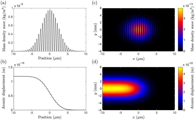
Figure 1: (Color online) Simulation results for a Gaussian light pulse having electromagnetic energy $U_{0}=1$ $\mu$J, vacuum wavelength $\lambda_{0}=1550$ nm, and $\Delta t_{\mathrm{FWHM}}=27$ fs. Panel (a) shows the MDW and (b) shows the atomic displacements of a one-dimensional pulse with energy $U_{0}$ per cross-sectional area of diameter $d=100$ $\mu$m. The phase and group refractive indices of the material for the central frequency are $n_{\mathrm{p}}=1.5$ and $n_{\mathrm{g}}=2$. These parameters are close to technological feasibility limit but they are suitable for our needs to visualize the node structure of the MDW. Panel (c) shows the atomic mass density of the MDW and (d) shows the atomic displacements of the MDW in the plane $z=0$ m for a three-dimensional light pulse having finite lateral dimensions.

Next, we use the OCD model to simulate the propagation of one- and three-dimensional Gaussian light pulses in a linearly dispersive material. These simulations aim at illustrating the node structure of the MDW and the related actual atomic displacements. The field of a Gaussian light pulse is modeled using Eq. (4). For the pulse, we use a vacuum wavelength of $\lambda_{0}=1550$ nm and a total electromagnetic energy of $U_{0}=1$ $\mu$J. In our example, the relative spectral width of the pulse is $\Delta\omega/\omega_{0}=\Delta k_{0}/k_{0}=0.05$, which corresponds to the temporal FWHM of $\Delta t_{\mathrm{FWHM}}=27$ fs. This small value is close to the feasibility limit and it is used here to make the node structure of the MDW visible in the same length scale with the pulse envelope. The spatial discretization used in the simulations is $h_{x}=\lambda/40$, where $\lambda=\lambda_{0}/n_{\mathrm{p}}$ is the wavelength in the medium, and the temporal discretization is $h_{t}=2\pi/(40\omega_{0})$. This discretization is sufficiently dense when compared to the scale of the harmonic cycle.

In the simulations of this subsection, we use an artificial example material that is suitable for our visualization needs. The refractive indices of the example material at the central frequency $\omega_{0}=2\pi c/\lambda_{0}$ are given by $n_{\mathrm{p}}=1.5$ and $n_{\mathrm{g}}=2$. The value of the phase refractive index is close to typical values for glasses but the group refractive index has been made larger for visualization needs. In the simulations, we assume a circular cross-sectional area $A=\pi(d/2)^{2}$ of diameter $d=100$ $\mu$m. This cross section is large enough so that the resulting maximum value $3.3\times 10^{11}$ W/cm² of the irradiance averaged over the harmonic cycle does not exceed the bulk value of the breakdown threshold irradiance of many common materials, e.g., the value of $5.0\times 10^{11}$ reported for fused silica [35]. For the equilibrium mass density of the material, we use a value of $\rho_{0}=2400$ kg/m³. The material is also assumed to be isotropic having a bulk modulus of $B=50$ GPa and a shear modulus of $G=25$ GPa. These material parameter values are close to typical values of the corresponding quantities for glass.

The position dependence of the MDW obtained as a result of the simulation is depicted in Fig. 1(a) when the center of the Gaussian light pulse is propagating to right at the position $x=0$ $\mu$m. The MDW driven by the optoelastic forces follows from solving Newton’s equation of motion in Eq. (5) and it equals the difference $\rho_{\text{\tiny MDW}}(\mathbf{r},t)=\rho_{\mathrm{a}}(\mathbf{r},t)-\rho_{0}$ of the perturbed mass density $\rho_{\mathrm{a}}(\mathbf{r},t)$ and the equilibrium mass density $\rho_{0}$. The nodes and the envelope of the MDW both follow the shape of the Gaussian pulse as expected. The total transferred mass of the light pulse can be obtained by the volume integral of the MDW mass density in Fig. 1(a). The resulting numerical value of the transferred mass is $2.23\times 10^{-23}$ kg. When this value is divided by the photon number of the pulse, $N_{0}=U_{0}/\hbar\omega_{0}=7.8\times 10^{12}$, we then obtain the value of $1.60$ eV/$c^{2}$ for the transferred mass per photon. This equals the MP quasiparticle value on the right in Eq. (11) within the relative error of $10^{-4}$.

The position dependence of the atomic displacements is shown in Fig. 1(b). These atomic displacements correspond to the MDW in Fig. 1(a). On the right of $x=7$ $\mu$m, the atomic displacement is zero since the leading edge of the pulse propagating to right at $x=7$ $\mu$m has not yet reached this area. Behind the pulse on the left of $x=-7$ $\mu$m, the atomic displacement has obtained a nonzero constant value of $r_{\mathrm{a,max}}=1.18\times 10^{-18}$ m. This is equal to $r_{\mathrm{a,max}}=\delta M/(\rho_{0}A)$, where $\delta M$ is the total transferred mass of the light pulse in Eq. (11). As the atoms behind the pulse have been shifted forwards and the atoms on the right of the pulse are still at their original equilibrium positions, the atoms are more densely spaced at the position of the light pulse. This local increase in the density of atoms is the origin of the MDW in Fig. 1(a). At an arbitrary time, the momentum of atoms in the MDW is obtained as an integral of the classical momentum density of atoms given in Eq. (10).

We also simulate the MDW and the atomic displacements resulting from the propagation of a three-dimensional Gaussian light pulse. This light pulse is obtained from the one-dimensional pulse in Eq. (4) by adding additional $y$ and $z$ dependencies using factors $e^{-(\Delta k_{y})^{2}y^{2}/2}$ and $e^{-(\Delta k_{z})^{2}z^{2}/2}$. Therefore, this light pulse is only an approximative solution of Maxwell’s equations. However, as reasoned in Ref. [2], this approximation becomes accurate in the limit where $\Delta k_{y}$ and $\Delta k_{z}$ are small compared to the wave number in the medium, given by $k_{\mathrm{0,med}}=n_{\mathrm{p}}k_{0}$. Here we use relatively small values $\Delta k_{y}=\Delta k_{z}=10^{-4}k_{0}$, which make this approximation sufficiently accurate for our visualization purposes.

The MDW of the three-dimensional Gaussian light pulse is illustrated in Fig. 1(c) by a contour plot in the plane $z=0$ m. The main difference between the three- and one-dimensional light pulses is formed by the finite lateral dimensions of the three-dimensional pulse as described above. This can also be seen in the MDW in Fig. 1(c), where the atomic density of the MDW becomes zero for increasing and decreasing values of $y$. From the lateral dimensions used and the corresponding smaller value of the energy per cross-sectional area, it also follows that the values of the atomic density of the MDW in Fig. 1(c) are smaller than the corresponding values of the one-dimensional MDW in Fig. 1(a)

Figure 1(d) shows the contour plot of the $x$ component of the atomic displacements resulting from the propagation of the three-dimensional Gaussian pulse in the plane $z=0$ m. These atomic displacements correspond to the MDW in Fig. 1(c). As a result of the smaller value of the energy per cross-sectional area, the values of the atomic displacement in Fig. 1(d) are also smaller than the values in the one-dimensional case in Fig. 1(b).

4.2 Estimating atomic displacements of the MDW in silicon

Next, we study the dependence of the atomic displacement of the MDW on the pulse energy and on the diameter of the pulse cross section. These simulations serve for designing experimental setups for the measurement of the transferred mass of a light pulse. We assume a one-dimensional Gaussian pulse in silicon and calculate the MDW shift for selected pulse energies, cross-sectional areas, and $\Delta t_{\mathrm{FWHM}}$. The simulated atomic displacements correspond to the experimental setup in which the pulse energy is propagating in a waveguide or an optical fiber as depicted in Fig. 2(a). Due to the interface effects, the physical cross-sectional area of the fiber is not equal to the cross-sectional area of our calculations. The effective core cross section of the fiber must account for the possible cladding layer, metallic coating, and other factors that govern the spreading of the pulse energy in the transverse direction. In quantitative predictive simulations, the waveguide dispersion should also be taken into account. All these factors can be included in the OCD simulations.

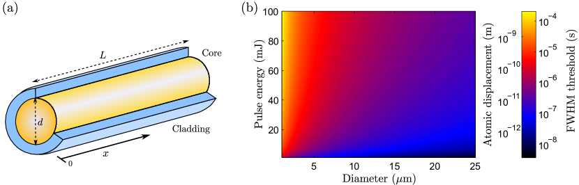
Figure 2: (Color online) (a) Schematic illustration of an optical fiber with a core diameter $d$ and length $L$. The transferred mass of the MDW can be calculated by measuring the shift of atoms on the surface of the waveguide at $x=L/2$ just after the light pulse has gone. (b) The dependence of the total atomic displacement of the MDW of a Gaussian light pulse in silicon on the pulse energy and on the diameter of the cross-sectional area of the pulse. The vacuum wavelength is $\lambda_{0}=1550$ nm and the corresponding phase and group refractive indices are $n_{\mathrm{p}}=3.4757$ and $n_{\mathrm{g}}=3.5997$. The second color-bar axis shows the threshold $\Delta t_{\mathrm{th}}$ of the pulse. It is obtained by requiring that the energy density of the pulse does not exceed the bulk value of the breakdown threshold irradiance.

For the phase and group refractive indices of crystalline silicon, we use literature values $n_{\mathrm{p}}=3.4757$ and $n_{\mathrm{g}}=3.5997$ respectively for $\lambda_{0}=1550$ nm [36]. For the density, we use $\rho_{0}=2329$ kg/m³ [37]. The elastic constants in the direction of the (100) plane used in the simulations were $C_{11}=165.7$ GPa, $C_{12}=63.9$ GPa, and $C_{44}=79.6$ GPa [38]. These elastic constants give for the bulk modulus a value of $B=(C_{11}+2C_{12})/3=97.8$ GPa and for the shear modulus a value of $G=C_{44}=79.6$ GPa.

Figure 2(b) depicts the dependence of the atomic displacement on the pulse energy and on the diameter of the cross-sectional area. Here we assume much longer pulses than above, typically $\Delta t_{\mathrm{FWHM}}>1$ ns. Therefore, the correspondence between the MP and the OCD models is very accurate. Thus we use the quasiparticle model result $r_{\mathrm{a,max}}=\delta M/(\rho_{0}A)$ for the maximum atomic displacement $r_{\mathrm{a,max}}$. We use $\delta M=(n_{\mathrm{p}}n_{\mathrm{g}}-1)U_{0}/c^{2}$ and $A=\pi(d/2)^{2}$, where $d$ is the diameter of the cross-sectional area, to obtain $r_{\mathrm{a,max}}=(n_{\mathrm{p}}n_{\mathrm{g}}-1)U_{0}/[c^{2}\rho_{0}\pi(d/2)^{2}]$. The atomic displacement depends linearly on the pulse energy and it is inversely proportional to the cross-sectional area. Accordingly, one can see in Fig. 2(b) that the atomic displacement is large for high pulse energies and for small cross-sectional areas.

4.2.1 Influence of the material breakdown irradiance

We also represent in Fig. 2(b) the minimum $\Delta t_{\mathrm{FWHM}}$ of a Gaussian pulse that is needed to produce the corresponding atomic displacement without exceeding the bulk value of the breakdown threshold irradiance of the pertinent material. Using the total electromagnetic pulse energy denoted by $U_{0}$, and the cross-sectional area of the pulse $A=\pi(d/2)^{2}$, this threshold $\Delta t_{\mathrm{FWHM}}$, denoted by $\Delta t_{\mathrm{th}}$, is calculated as $\Delta t_{\mathrm{th}}=2U_{0}/[\pi(d/2)^{2}I_{\mathrm{th}}]$. Here $I_{\mathrm{th}}$ is the bulk value of the breakdown threshold irradiance of the material. The corresponding value of the fluence is given by $F_{\mathrm{th}}=2U_{0}/[\pi(d/2)^{2}]$. The factor $2$ comes from the fact that the pulse is Gaussian instead of a top-hat pulse with constant irradiance. For silicon with $\lambda_{0}=1550$ nm, the bulk value of the breakdown threshold energy density $u_{\mathrm{th}}=13.3$ J/cm³ has been reported by Cowan [39]. This corresponds to the threshold irradiance of $I_{\mathrm{th}}=u_{\mathrm{th}}v_{\mathrm{g}}=1.11\times 10^{11}$ W/cm². These are values averaged over the harmonic cycle.

The calculated threshold $\Delta t_{\mathrm{th}}$ of a Gaussian pulse is presented by the second color-bar axis in Fig. 2(b). Using the formulas given above, the scaling between the atomic displacement and the threshold $\Delta t_{\mathrm{th}}$ is given by $r_{\mathrm{a,max}}/\Delta t_{\mathrm{th}}=(n_{\mathrm{p}}n_{\mathrm{g}}-1)I_{\mathrm{th}}/(2c^{2}\rho_{0})$. This indicates that, to obtain large atomic displacements for a given pulse energy, one should choose a material with a high refractive index, high breakdown threshold irradiance, and relatively small mass density. Fig. 2(b) shows that, in order to obtain atomic displacements larger than $1$ nm in silicon without breaking the material, a pulse width larger than $\Delta t_{\mathrm{th}}=33$ $\mu$s must be used.

4.2.2 Displacement of atoms due to optical absorption

In the simulations above, we have neglected possible momentum transfer and shift of atoms caused by light absorption. To estimate the accuracy of this approximation, we next calculate the total atomic displacement and the atomic velocity caused by the optical absorption. The mass of a cylindrical medium block with a diameter $d$ and length $L$, i.e., the core of the fiber in Fig. 2(a), is given by $M=\rho_{0}\pi(d/2)^{2}L$. The momentum absorbed by the cylinder is given by $P_{\mathrm{abs}}=(1-e^{-\alpha L})n_{\mathrm{p}}U_{0}/c\approx\alpha Ln_{\mathrm{p}}U_{0}/c$, where $\alpha$ is the small absorption coefficient of the medium. The velocity of the medium block resulting from the absorption is then $V_{\mathrm{abs}}=P_{\mathrm{abs}}/M\approx\alpha n_{\mathrm{p}}U_{0}/[c\rho_{0}\pi(d/2)^{2}]$. In the time scale of $\Delta t_{\mathrm{FWHM}}$, this gives an atomic displacement of $X_{\mathrm{abs}}=V_{\mathrm{abs}}\Delta t_{\mathrm{FWHM}}$.

For single-crystal silicon, absorption is very low at $\lambda_{0}=1550$ nm. Schinke et al. [40] and Green [41] have given for $\lambda_{0}=1450$ nm give $\alpha\approx 10^{-8}$ cm^-1 and the absorption decreases towards $\lambda_{0}=1550$ nm. Thus, we conservatively estimate $\alpha=10^{-8}$ cm^-1. We use $\Delta t_{\mathrm{FWHM}}=\Delta t_{\mathrm{th}}=33$ $\mu$s and $d=2.5$ $\mu$m corresponding to $r_{\mathrm{a,max}}=1.0$ nm atomic displacement due to the MDW. By solving the threshold pulse energy from $\Delta t_{\mathrm{th}}=2U_{0}/[\pi(d/2)^{2}I_{\mathrm{th}}]$, we then obtain $U_{0}=90$ mJ. The corresponding velocity of atoms is $V_{\mathrm{abs}}=9.1\times 10^{-8}$ m/s and, in the time intervall of $\Delta t_{\mathrm{th}}$, the resulting atomic displacement is given by $X_{\mathrm{abs}}=3.0$ pm. Thus the atomic displacement due to optical absorption is vastly smaller than $r_{\mathrm{a,max}}=1.0$ nm following from the MDW. We conclude that optical absorption should not prevent measurements of the atomic displacements due to the MDW. The experimental measurement of the transferred mass of the MDW is feasible in the light of these results.

4.2.3 Thermal expansion following from optical absorption

Next, we consider thermal expansion following from the optical absorption. If the rate of absorption of optical energy remains low compared to the total field energy, as is the case in our example, the absorbed energy per unit length is approximately constant. This energy will be converted into heat and it leads to a local equilibrium lattice and electronic temperature in a relaxation time that is of the order of picoseconds. This elevated equilibrium temperature then corresponds to an increased lattice constant and gives rise to an elastic force that starts to shift atoms towards their new equilibrium positions. Thus, the thermal expansion takes place at the velocity of sound and comes behind the optical pulse and the MDW shift of atoms which is a shock wave propagating at the velocity of light. Using the literature values for the specific-heat capacity and thermal-expansion coefficients, it can be estimated that the thermal expansion does not lead to measurable atomic displacements in the middle part of the fiber in a time $\Delta t_{\mathrm{FWHM}}$ which is shorter than the time the sound waves need to travel through the fiber. Thermal expansion is also related to the longitudinal relaxation studied below.

4.2.4 Transverse relaxation

In measuring the transferred mass of the MDW, one also has to account for the relaxation of the atomic displacements of the MDW by phonons. This relaxation is governed by the elastic forces in the OCD model and it takes place at the velocity of sound.

The relaxation effect has been represented in Ref. [2]. If a three-dimensional light pulse propagates in the core of an optical fiber that has a cladding, the MDW displaces atoms as shown in Fig. 1(d). Along the path of the MP, the atoms are displaced forwards. The atoms in the surrounding layers are not shifted forwards since they do not feel the optical force. This gives rise to a shear strain field along the path of the MP. By the transverse relaxation we mean in the following the relaxation of the strain field so that atoms in the displaced region (core) are shifted backwards and atoms in the surrounding layers (cladding) are shifted forwards. After this relaxation, the longitudinal strain becomes constant across the cross section of the waveguide.

In optical fibers, the transverse relaxation of the strain field is fast since the distances to be traveled by phonons in the transverse direction are very short. The longitudinal velocity of sound in silicon is given by $v_{\parallel}=\sqrt{C_{11}/\rho_{0}}=8435$ m/s. The time that it takes for a sound wave to propagate, e.g., a distance of $1$ mm is $1.2$ ns. This is a short time when compared to the time scale of $\Delta t_{\mathrm{FWHM}}=33$ $\mu$s used above. Thus, the transverse relaxation takes place in a time scale that is shorter than the passing time of the pulse. Atoms are accordingly displaced in the longitudinal direction by the same amount in the middle and at the surface of the waveguide. When the transverse relaxation has taken place, the atomic displacement is constant in the transverse plane and it is reduced to $r_{\mathrm{a,relaxed}}=r_{\mathrm{a,max}}\rho_{0}A/(\rho_{\mathrm{eff}}A_{\mathrm{tot}})$. Here $A_{\mathrm{tot}}$ is the total cross-sectional area of all layers in the given transverse plane and $\rho_{\mathrm{eff}}$ is the effective mass density of the cross-sectional area given by $\rho_{\mathrm{eff}}=\sum_{i}\rho_{i}A_{i}/A_{\mathrm{tot}}$. Here the sum is taken over all material layers. The densities and cross-sectional areas of the corresponding layers are denoted by $\rho_{i}$ and $A_{i}$.

In summary, the time needed for the transverse relaxation is much shorter than the pulse width in the time domain $\Delta t_{\mathrm{FWHM}}$ for structures where the atomic displacement is potentially measurable. It is thus advantageous to keep the waveguide diameter as small as possible. The tradeoff is to be made by considering the effectivity of the coupling of the light source to the waveguide and the technical processing aspects of fabricating the waveguide. Within these engineering feasibility limits, the narrower the waveguide is, the larger is the atomic displacement and the breakdown of the material can be prevented by increasing the pulse width $\Delta t_{\mathrm{FWHM}}$. There is however a further limiting factor that will set a limit for increasing $\Delta t_{\mathrm{FWHM}}$, based on the longitudinal relaxation. This will be described in the next subsection.

4.2.5 Longitudinal relaxation

After the transverse relaxation is complete, further relaxation starts by sound waves from the ends of the fiber. If the fiber is long enough, the relaxation does not have time to reach the middle part of the fiber where the atomic displacement is to be measured. In the time scale of $\Delta t_{\mathrm{FWHM}}=33$ $\mu$s, the distance traveled by sound in silicon is $28$ cm. A fiber with length $L>56$ cm is thus enough to avoid the longitudinal relaxation from influencing the measured atomic displacement if the displacement in the middle part of the fiber is measured immediately after the light pulse has passed this zone.

5 Conclusions

In conclusion, we have generalized the recently developed MP theory of light for the study of light propagation in dispersive media. We have compared the related OCD model to the MP quasiparticle picture. Our results show how the total energy and momentum are shared by the electromagnetic field and the medium atoms in the MDW. Both the MP quasiparticle picture and the OCD approach lead to transfer of mass with the light pulse. The transfer of mass comes from the shift of atoms in the medium and it is expected to be experimentally feasible to measure. To facilitate the planning of measurements, we have carried out simulations of how the atomic displacements due to the MDW changes as a function of space and time in a simple silicon waveguide structure. In the simulations, we have considered different waveguide cross sections and optical pulse widths. We have also accounted for the breakdown threshold irradiance of silicon, which is one of the main limiting factors in possible experimental setups as the electromagnetic energy density in the medium cannot be made arbitrarily large without damaging the medium. Using the OCD model, it is also possible to perform more detailed simulations, which account for the waveguide dispersion and the spreading of the pulse energy in the transverse direction. These simulations are a topic of further work.

- [1] L. D. Landau, E. M. Lifshitz, and L. P. Pitaevskii, Electrodynamics of Continuous Media, Pergamon, Oxford (1984).
- [2] M. Partanen, T. Häyrynen, J. Oksanen, and J. Tulkki, “Photon mass drag and the momentum of light in a medium,” Phys. Rev. A 95, 063850 (2017).
- [3] M. Partanen and J. Tulkki, “Mass-polariton theory of light in dispersive media,” Phys. Rev. A 96, 063834 (2017).
- [4] U. Leonhardt, “Momentum in an uncertain light,” Nature 444, 823 (2006).
- [5] A. Cho, “Century-long debate over momentum of light resolved?” Science 327, 1067 (2010).
- [6] R. N. C. Pfeifer, T. A. Nieminen, N. R. Heckenberg, and H. Rubinsztein-Dunlop, “Colloquium: Momentum of an electromagnetic wave in dielectric media,” Rev. Mod. Phys. 79, 1197 (2007).
- [7] S. M. Barnett, “Resolution of the Abraham-Minkowski dilemma,” Phys. Rev. Lett. 104, 070401 (2010).
- [8] S. M. Barnett and R. Loudon, “The enigma of optical momentum in a medium,” Phil. Trans. R. Soc. A 368, 927 (2010).
- [9] U. Leonhardt, “Abraham and Minkowski momenta in the optically induced motion of fluids,” Phys. Rev. A 90, 033801 (2014).
- [10] P. L. Saldanha and J. S. O. Filho, “Hidden momentum and the Abraham-Minkowski debate,” Phys. Rev. A 95, 043804 (2017).
- [11] T. Ramos, G. F. Rubilar, and Y. N. Obukhov, “First principles approach to the Abraham-Minkowski controversy for the momentum of light in general linear non-dispersive media,” J. Opt. 17, 025611 (2015).
- [12] I. Brevik, “Minkowski momentum resulting from a vacuum-medium mapping procedure, and a brief review of Minkowski momentum experiments,” Ann. Phys. 377, 10 (2017).
- [13] M. Mansuripur, “Resolution of the Abraham-Minkowski controversy,” Opt. Commun. 283, 1997 (2010).
- [14] B. A. Kemp, “Resolution of the Abraham-Minkowski debate: Implications for the electromagnetic wave theory of light in matter,” J. Appl. Phys. 109, 111101 (2011).
- [15] H. Choi, M. Park, D. S. Elliott, and K. Oh, “Optomechanical measurement of the Abraham force in an adiabatic liquid-core optical-fiber waveguide,” Phys. Rev. A 95, 053817 (2017).
- [16] G. K. Campbell, A. E. Leanhardt, J. Mun, M. Boyd, E. W. Streed, W. Ketterle, and D. E. Pritchard, “Photon recoil momentum in dispersive media,” Phys. Rev. Lett. 94, 170403 (2005).
- [17] R. E. Sapiro, R. Zhang, and G. Raithel, “Atom interferometry using Kapitza-Dirac scattering in a magnetic trap,” Phys. Rev. A 79, 043630 (2009).
- [18] R. V. Jones and J. C. S. Richards, “The pressure of radiation in a refracting medium,” Proc. R. Soc. Lond. A 221, 480 (1954).
- [19] R. V. Jones and B. Leslie, “The measurement of optical radiation pressure in dispersive media,” Proc. R. Soc. Lond. A 360, 347 (1978).
- [20] G. B. Walker and D. G. Lahoz, “Experimental observation of Abraham force in a dielectric,” Nature 253, 339 (1975).
- [21] W. She, J. Yu, and R. Feng, “Observation of a push force on the end face of a nanometer silica filament exerted by outgoing light,” Phys. Rev. Lett. 101, 243601 (2008).
- [22] L. Zhang, W. She, N. Peng, and U. Leonhardt, “Experimental evidence for Abraham pressure of light,” New J. Phys. 17, 053035 (2015).
- [23] N. G. C. Astrath, L. C. Malacarne, M. L. Baesso, G. V. B. Lukasievicz, and S. E. Bialkowski, “Unravelling the effects of radiation forces in water,” Nat. Commun. 5, 4363 (2014).
- [24] A. Ashkin and J. M. Dziedzic, “Radiation pressure on a free liquid surface,” Phys. Rev. Lett. 30, 139 (1973).
- [25] A. Casner and J.-P. Delville, “Giant deformations of a liquid-liquid interface induced by the optical radiation pressure,” Phys. Rev. Lett. 87, 054503 (2001).
- [26] I. Brevik, “Experiments in phenomenological electrodynamics and the electromagnetic energy-momentum tensor,” Phys. Rep. 52, 133 (1979).
- [27] M. Abraham, “Zur Elektrodynamik bewegter Körper,” Rend. Circ. Matem. Palermo 28, 1 (1909).
- [28] M. Abraham, “Sull’elettrodinamica di Minkowski,” Rend. Circ. Matem. Palermo 30, 33 (1910).
- [29] H. Minkowski, “Die Grundgleichungen für die elektromagnetischen Vorgänge in bewegten Körpern,” Nachr. Ges. Wiss. Göttn Math.-Phys. Kl. 53 (1908), reprinted in Math. Ann. 68, 472 (1910).
- [30] M. Partanen, T. Häyrynen, J. Oksanen, and J. Tulkki, “Photon momentum and optical forces in cavities,” Proc. SPIE 9742, 974217 (2016).
- [31] M. Partanen and J. Tulkki, “Momentum and rest mass of the covariant state of light in a medium,” Proc. SPIE 10098, 100980P (2017).
- [32] D. J. Griffiths, Introduction to Electrodynamics, Prentice-Hall, Upper Saddle River, NJ (1998).
- [33] C. Kittel, Introduction to Solid State Physics, Wiley, Hoboken, NJ (2005).
- [34] P. W. Milonni and R. W. Boyd, “Momentum of light in a dielectric medium,” Adv. Opt. Photon. 2, 519 (2010).
- [35] A. Smith, B. Do, and M. Soderlund, “Deterministic nanosecond laser-induced breakdown thresholds in pure and Yb3+ doped fused silica,” Proc. SPIE 6453, 645317 (2007).
- [36] H. H. Li, “Refractive index of silicon and germanium and its wavelength and temperature derivatives,” J. Phys. Chem. Ref. Data 9, 561 (1980).
- [37] D. R. Lide, ed., CRC Handbook of Chemistry and Physics, CRC Press, Boca Raton, FL (2004).
- [38] M. A. Hopcroft, W. D. Nix, and T. W. Kenny, “What is the Young’s modulus of silicon?” J. Microelectromech. Syst. 19, 229 (2010).
- [39] B. Cowan, “Optical damage threshold of silicon for ultrafast infrared pulses,” AIP Conf. Proc. 877, 837 (2006).
- [40] C. Schinke, P. C. Peest, J. Schmidt, R. Brendel, K. Bothe, M. R. Vogt, I. Kröger, S. Winter, A. Schirmacher, S. Lim, H. T. Nguyen, and D. MacDonald, “Uncertainty analysis for the coefficient of band-to-band absorption of crystalline silicon,” AIP Adv. 5, 067168 (2015).
- [41] M. A. Green, “Self-consistent optical parameters of intrinsic silicon at 300K including temperature coefficients,” Sol. Energ. Mat. Sol. Cells 92, 1305 (2008).