Abstract

This paper presents a distance-based discriminative framework for learning with probability distributions. Instead of using kernel mean embeddings or generalized radial basis kernels, we introduce embeddings based on dissimilarity of distributions to some reference distributions denoted as templates. Our framework extends the theory of similarity of Balcan et al. , (2008) to the population distribution case and we show that, for some learning problems, some dissimilarity on distribution achieves low-error linear decision functions with high probability. Our key result is to prove that the theory also holds for empirical distributions. Algorithmically, the proposed approach consists in computing a mapping based on pairwise dissimilarity where learning a linear decision function is amenable. Our experimental results show that the Wasserstein distance embedding performs better than kernel mean embeddings and computing Wasserstein distance is far more tractable than estimating pairwise Kullback-Leibler divergence of empirical distributions.

1 Introduction

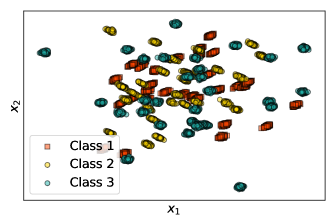
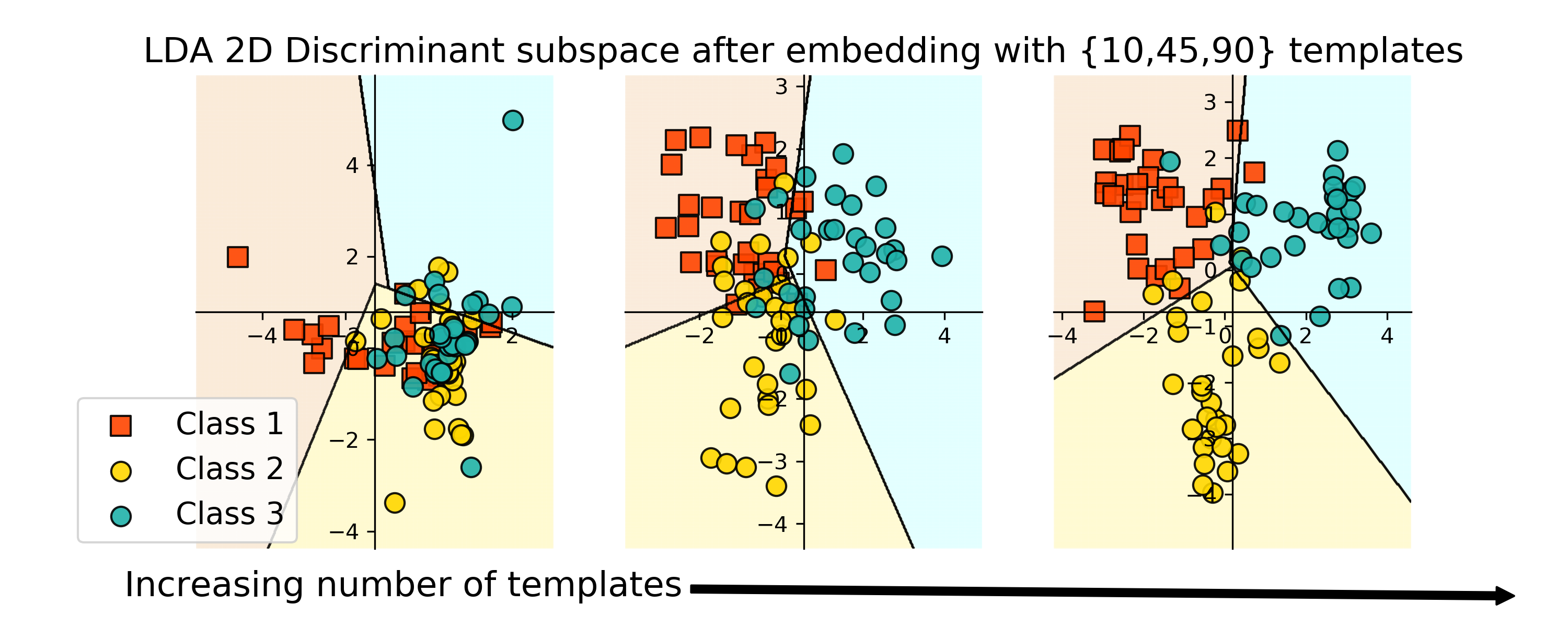
Figure 1: Illustrating the principle of the dissimilarity-based distribution embedding. We want to discriminate empirical normal distributions in $\mathbb{R}^{2}$; their discriminative feature being the correlation between the two variables. An example of these normal distributions are given in the left panel. The proposed approach consists in computing a embedding based on the dissimilarity of all these empirical distributions (the blobs) to few of, them that serve as templates. Our theoretical results show that if we take enough templates and there is enough samples in each template then with high-probability, we can learn a linear separator that yields few errors. This is illustrated in the 3 other panels in which we represent each of the original distribution as a point after projection in an discriminant 2D space of the embeddings. From left to right, the dissimilarity embedding respectively considers $10$, $45$ and $90$ templates and we can indeed visualize that using more templates improve separability.

Most discriminative machine learning algorithms have focused on learning problems where inputs can be represented as feature vectors of fixed dimensions. This is the case of popular algorithms like support vector machines (Schölkopf & Smola,, 2002) or random forest (Breiman,, 2001). However, there exists several practical situations where it makes more sense to consider input data as set of distributions or empirical distributions instead of a larger collection of single vector. As an example, multiple instance learning (Dietterich et al. ,, 1997) can be seen as learning of a bag of feature vectors and each bag can be interpreted as samples from an underlying unknown distribution. Applications related to political sciences (Flaxman et al. ,, 2015) or astrophysics Ntampaka et al. , (2015) have also considered this learning from distribution point of view for solving some specific machine learning problems. This paper also addresses the problem of learning decision functions that discriminate distributions.

Traditional approaches for learning from distributions is to consider reproducing kernel Hilbert spaces (RKHS) and associated kernels on distributions. In this larger context, several kernels on distributions have been proposed in the literature such as the probability product kernel (Jebara et al. ,, 2004), the Battarachya kernel (Bhattacharyya,, 1943) or the Hilbertian kernel on probability measures of Hein & Bousquet, (2005). Another elegant approach for kernel-based distribution learning has been proposedby Muandet et al. , (2012). It consists in defining an explicit embedding of a distribution as a mean embedding in a RKHS. Interestingly, if the kernel of the RKHS satisfies some mild conditions then all the information about the distribution is preserved by this mean embedding. Then owing to this RKHS embedding, all the machinery associated to kernel machines can be deployed for learning from these (embedded) distributions.

By leveraging on the flurry of distances between distributions (Sriperumbudur et al. ,, 2010), it is also possible to build definite positive kernel by considering generalized radial basis function kernels of the form

$$K(\mu,\mu^{\prime})=e^{-\sigma d^{2}(\mu,\mu^{\prime})},$$ (1)

where $\mu$ and $\mu^{\prime}$ are two distributions, $\sigma>0$ a parameter of the kernel and $d(\cdot,\cdot)$ a distance between two distributions satisfying some appropriate properties so as to make $K$ definite positive (Haasdonk & Bahlmann,, 2004).

As we can see, most works in the literature address the question of discriminating distributions by considering either implicit or explicit kernel embeddings. However, is this really necessary? Our observation is that there are many advantages of directly using distances or even dissimilarities between distributions for learning. It would avoid the need for two-stage approaches, computing the distance and then the kernel, as proposed by Póczos et al. , (2013) for distribution regression or estimating the distribution and computing the kernel as introduced by Sutherland et al. , (2012). Using kernels limits the choice of distribution distances as the resulting kernel has to be definite positive. For instance, Póczos et al. , (2012) used Reyni divergences for building generalized RBF kernel that turns out to be non-positive. For the same reason, the celebrated and widely used Kullback-Leibler divergence does not qualify for being used in a kernel. This work aims at showing that learning from distributions with distances or even dissimilarity is indeed possible. Among all available distances on distributions, we focus our analysis on Wasserstein distances which come with several relevant properties, that we will highlight later, compared to other ones (e.g Kullback-Leibler divergence).

Our contributions, depicted graphically in Figure 1, are the following : (a) We show that by following the underlooked works of Balcan et al. , (2008), learning to discriminate population distributions with dissimilarity functions comes at no expense. While this might be considered a straightforward extension, we are not aware of any work making this connection. (b) Our key theoretical contribution is to show that Balcan’s framework also holds for empirical distributions if the used dissimilarity function is endowed with nice convergence properties of the distance of the empirical distribution to the true ones. (c) While these convergence bounds have already been exhibited for distances such as the Wasserstein distance or MMD, we prove that this is also the case for the Bures-Wasserstein metric.(d) Empirically, we illustrate the benefits of using this Wasserstein-based dissimilarity functions compared to kernel or MMD distances in some simulated and real-world vision problem, including 3D point cloud classification task.

2 Framework

In this section, we introduce the global setting and present the theory of learning with dissimilarity functions of Balcan et al. , (2008).

2.1 Setting

Define $\mathcal{X}$ as an non-empty subset of $\mathbb{R}^{d}$ and let $\mathbb{P}$ denotes the set of all probability measures on a measurable space $(\mathcal{X},\mathcal{A})$, where $\mathcal{A}$ is $\sigma$-algebra of subsets of $\mathcal{X}$. Given a training set $\{\mu_{i},y_{i}\}_{i=1}^{n}$, where $\mu_{i}\in\mathbb{P}$ and $y_{i}\in\{-1,1\}$, drawn i.i.d from a probability distribution $P$ on $\mathbb{P}\times\{-1,1\}$, our objective is to learn a decision function $h:\mathbb{P}\mapsto\{-1,1\}$ that predicts the most accurately as possible the label associated to a novel measure $\mu$. In summary, our goal is to learn to classify probability distributions from a supervised setting. While we focus on a binary classification, the framework we consider and analyze can be extended to multi-class classification.

2.2 Dissimilarity function

Most learning algorithms for distributions are based on reproducing kernel Hilbert spaces and leverage on kernel value $k(\mu,\mu^{\prime})$ between two distributions where $k(\cdot,\cdot)$ is the kernel of a given RKHS.

We depart from this approach and instead, we consider learning algorithms that are built from pairwise dissimilarity measures between distributions. Subsequent definitions and theorems are recalled from Balcan et al. , (2008) and adapted so as to suit our definition of bounded dissimilarity.

Definition 1.

A dissimilarity function over $\mathbb{P}$ is any pairwise function $\mathcal{D}:\mathbb{P}\times\mathbb{P}\mapsto[0,M]$.

While this definition emcompasses many functions, given two probability distributions $\mu$ and $\mu^{\prime}$, we expect $\mathcal{D}(\mu,\mu^{\prime})$ to be large when the two distributions are “dissimilar” and to be equal to $0$ when they are similar. As such any bounded distance over $\mathbb{P}$ fits into our notion of dissimilarity, eventually after rescaling. Note that unbounded distance which is clipped above $M$ also fits this definition of dissimilarity.

Now, we introduce the definition that characterizes dissimilarity function that allows one to learn a decision function producing low error for a given learning task.

Definition 2.

Balcan et al. , (2008) A dissimilarity function $\mathcal{D}$ is a $(\epsilon,\gamma)$-good dissimilarity function for a learning problem $\mathbf{L}$ if there exists a bounded weighting function $w$ over $\mathbb{P}$, with $w(\mu)\in[0,1]$ for all $\mu\in\mathbb{P}$, such that a least $1-\epsilon$ probability mass of distribution examples $\mu$ satisfy : $\mathbf{E}_{\mu^{\prime}\sim P}[w(\mu^{\prime})\mathcal{D}(\mu,\mu^{\prime})|\ell(\mu)=\ell(\mu^{\prime})]+\gamma\leq\mathbf{E}_{\mu^{\prime}\sim P}\left[w(\mu^{\prime})\mathcal{D}(\mu,\mu^{\prime})|\ell(\mu)\neq\ell(\mu^{\prime})\right].$ The function $\ell(\mu)$ denotes the true labelling function that maps $\mu$ to its labels $y$.

In other words, this definition translates into: a dissimilarity function is “good” if with high-probability, the weighted average of the dissimilarity of one distribution to those of the same label is smaller with a margin $\gamma$ to the dissimilarity of distributions from the other class.

As stated in a theorem of Balcan et al. , (2008), such a good dissimilarity function can be used to define an explicit mapping of a distribution into a space. Interestingly, it can be shown that there exists in that space a linear separator that produces low errors.

Theorem 1.

Balcan et al. , (2008) if $\mathcal{D}$ is an $(\epsilon,\gamma)$-good dissimilarity function, then if one draws a set $S$ from $\mathbb{P}$ containing $n=(\frac{4M}{\gamma})^{2}\log(\frac{2}{\delta})$ positive examples $S^{+}=\{\nu_{1},\cdots,\nu_{n}\}$ and $n$ negative examples $S^{-}=\{\zeta_{1},\cdots,\zeta_{n}\}$, then with probability $1-\delta$, the mapping $\rho_{S}:\mathbb{P}\mapsto\mathbb{R}^{2n}$ defined as $\rho_{S}(\mu)=(\mathcal{D}(\mu,\nu_{1}),\cdots,\mathcal{D}(\mu,\nu_{n}),\mathcal{D}(\mu,\zeta_{1}),\cdots,\mathcal{D}(\mu,\zeta_{n}))$ has the property that the induced distribution $\rho_{S}(\mathbb{P})$ in $\mathbb{R}^{2n}$ has a separator of error at most $\epsilon+\delta$ at margin at least $\gamma/4$.

The above described framework shows that under some mild conditions on a dissimilarity function and if we consider population distributions, then we can benefit from the mapping $\rho_{S}$. However, in practice, we do have access only to empirical version of these distributions. Our key theoretical contribution in Section 3 proves that if the number of distributions $n$ is large enough and enough samples are obtained from each of these distributions, then this framework is applicable with theoretical guarantees to empirical distributions.

3 Learning with empirical distributions

In what follows, we formally show under which conditions an $(\epsilon,\gamma)$-good dissimilarity function for some learning problems, applied to empirical distributions also produces a mapping inducing low-error linear separator.

Suppose that we have at our disposal a dataset composed of $\{\mu_{i},y_{i}=1\}_{i=1}^{n}$ where each $\mu_{i}$ is a distribution. However, each $\mu_{i}$ is not observed directly but instead we observe it empirical version $\hat{\mu}_{i}=\frac{1}{N_{i}}\sum_{j=1}^{N_{i}}\delta_{\mathbf{x}_{i,j}}$ with $\mathbf{x}_{i,1},\mathbf{x}_{i,2},\cdots\mathbf{x}_{i,N_{i}}\stackrel{{\scriptstyle i.i.d}}{{\sim}}\mu_{i}$. For a sake of simplicity, we assume in the sequel that the number of samples for all distributions are equal to $N$. Suppose that we consider a dissimilarity $\mathcal{D}$ and that there exist a function $g_{1}$ such that $\mathcal{D}$ satisfies a property of the form $\mathbf{P}\Big{(}\mathcal{D}(\mu,\hat{\mu})>\epsilon\Big{)}\leq g_{1}(K,N,\epsilon,d)$ then following theorem holds:

Theorem 2.

For a given learning problem, if the dissimilarity $\mathcal{D}$ is an $(\epsilon,\gamma)$-good dissimilarity function on population distributions, with $w(\mu)=1,\,\,\forall\mu$ and $K$ a parameter depending on this dissimilarity then, for a parameter $\lambda\in(0,1)$, if one draws a set $S$ from $\mathbb{P}$ containing $n=\frac{32M^{2}}{\gamma^{2}}\log(\frac{2}{\delta^{2}(1-\lambda)})$ positive examples $S^{+}=\{\nu_{1},\cdots,\nu_{n}\}$ and $n$ negative examples $S^{-}=\{\zeta_{1},\cdots,\zeta_{n}\}$, and from each distribution $\nu_{i}$ or $\zeta_{i}$, one draws $N$ samples so that $\delta^{2}\lambda\geq Ng_{1}(K,N,\frac{\epsilon}{4},d)$ samples so as to build empirical distributions $\{\hat{\nu}_{i}\}$ or $\{\hat{\zeta}_{i}\}$, then with probability $1-\delta$, the mapping $\hat{\rho}_{S}:\mathbb{P}\mapsto\mathbb{R}^{2n}$ defined as

$$\hat{\rho}_{S}(\hat{\mu})=\frac{1}{M}(\mathcal{D}(\hat{\mu},\hat{\nu}_{1}),\cdots,\mathcal{D}(\hat{\mu},\hat{\nu}_{n}),\mathcal{D}(\hat{\mu},\hat{\zeta}_{1}),\cdots,\mathcal{D}(\hat{\mu},\hat{\zeta}_{n}))$$

has the property that the induced distribution $\rho_{S}(\mathbb{P})$ in $\mathbb{R}^{2n}$ has a separator of error at most $\epsilon+\delta$ and margin at least $\gamma/4$.

Let us point out some relevant insights from this theorem. At first, due to the use of empirical distributions instead of population one, the sample complexity of the learning problem increases for achieving similar error as in Theorem 1. Secondly, note that $\lambda$ has a trade-off role on the number $n$ of samples $\nu_{i}$ and $\zeta_{i}$ and the number of observations per distribution. Hence, for a fixed error $\epsilon+\delta$ at margin $\gamma/4$, having less samples per distribution has to be paid by sampling more observations.

The proof of Theorem 1 has been postponed to the appendix. It takes advantage of the following key technical result on empirical distributions.

Lemma 1.

Let $\mathcal{D}$ be a dissimilarity on $\mathbb{P}\times\mathbb{P}$ such that $\mathcal{D}$ is bounded by a constant $M$. Given a distribution $\mu\in\mathbb{P}$ of class $y$ and a set of independent distributions $\left\{\nu_{j}\right\}_{j=1}^{n}$, randomly drawn from $\mathbb{P}$, which have the same label $y$ and denote as $\hat{\mu}$ and $\{\hat{\nu}_{i}\}$ their empirical version composed of $N$ observations. Let us assume that there exists a function $g_{1}$ and a constant $K>0$ so that for any $\mu\in\mathbb{P}$, $\mathbf{P}\Big{(}\mathcal{D}(\mu,\hat{\mu})>\epsilon\Big{)}\leq g_{1}(K,N,\epsilon,d)$, with typically $g_{1}$ tends towards $0$ as $N$ or $\epsilon$ goes to $\infty$. The following concentration inequality holds for any $\epsilon>0$ :

$$\mathbf{P} \left(\left|\frac{1}{n}\sum_{i=1}^{n}\mathcal{D}(\hat{\mu},\hat{\nu}_{i})-\mathbf{E}_{\nu\sim\mathbb{P}}[\mathcal{D}(\mu,\nu)|\ell(\mu)=\ell(\nu)]\right|>\epsilon\right)~{}$$

$$\leq Ng_{1}(K,N,\frac{\epsilon}{4},d)+2e^{-n\frac{\epsilon^{2}}{2M^{2}}}.$$

This lemma tells us that, with high probability, the mean average of the dissimilarity between an empirical distribution and some other empirical distribution of the same class does not differ much from the expectation of this dissimilarity measured on population distributions. Interestingly, the bound on the probability is composed of two terms : the first one is related to the dissimilarity function between a distribution and its empirical version while the second one is due to the empirical version of the expectation (resulting thus from Hoeffding inequality). The detailed proof of this result is given in the supplementary material. Note that in order for the bound to be informative, we expect $g_{1}$ to have a negative exponential form in $N$. Another version of this lemma is proven in supplementary where the concentration inequality for the dissimilarity is on $|\mathcal{D}(\hat{\mu},\hat{\nu})-\mathcal{D}(\mu,\nu)|$.

From a theoretical point of view, there is only one reason for choosing one $(\epsilon,\gamma)$-good dissimilarity function on population distributions from another. The rationale would be to consider the dissimilarity function with the fastest rate of convergence of the concentration inequality $\text{Pr}(\mathcal{D}(\mu,\hat{\mu})>\epsilon)$, as this rate will impact the upper bound in Theorem 1.

From a more practical point of view, several factors may motivate the choice of a dissimilarity function : computational complexity of computing $\mathcal{D}(\hat{\mu}_{i},\hat{\mu}_{j})$, its empirical performance on a learning problem and adaptivity to different learning problems ( e.g without the need for carefully adapting its parameters to a new problem.)

4 ($\epsilon-\gamma$) Good dissimilarity for distributions

We are interested now in characterizing convergence properties of some dissimilarities (or distance or divergence) on probability distributions so as to make them fit into the framework. Mostly, we will focus our attention on divergences that can be computed in a non-parametric way.

4.1 Optimal transport distances

Based on the theory of optimal transport, these distances offer means to compare data probability distributions. More formally, assume that $\mathcal{X}$ is endowed with a metric $d_{\mathcal{X}}$. Let $p\in(0,\infty)$, and let $\mu\in\mathbb{P}$ and $\nu\in\mathbb{P}$ be two distributions with finite moments of order p (i.e. $\int_{\mathcal{X}}d_{\mathcal{X}}(x,x_{0})^{p}d\mu(x)<\infty$ for all $x_{0}$ in $\mathcal{X}$). then, the p-Wasserstein distance is defined as:

$$W_{p}(\mu,\nu)=\left(\inf_{\pi\in\Pi(\mu,\nu)}\iint_{\mathcal{X}\times\mathcal{X}}d_{\mathcal{X}}(x,y)^{p}d\pi(x,y)\right)^{\frac{1}{p}}.$$ (2)

Here, $\Pi(\mu,\nu)$ is the set of probabilistic couplings $\pi$ on $(\mu,\nu)$. As such, for every Borel subsets $A\subseteq\mathcal{X}$, we have that $\mu(A)=\pi(\mathcal{X}\times A)$ and $\nu(A)=\pi(A\times\mathcal{X})$. We refer to (Villani,, 2009, Chaper 6) for a complete and mathematically rigorous introduction on the topic. Note when $p=1$, the resulting distance belongs to the family of integral probability metrics Sriperumbudur et al. , (2010). OT has found numerous applications in machine learning domain such as multi-label classification (Frogner et al. ,, 2015), domain adaptation (Courty et al. ,, 2017) or generative models (Arjovsky et al. ,, 2017). Its efficiency comes from two major factors: i) it handles empirical data distributions without resorting first to parametric representations of the distributions ii) the geometry of the underlying space is leveraged through the embedding of the metric $d_{\mathcal{X}}$. In some very specific cases the solution of the infimum problem is analytic. For instance, in the case of two Gaussians $\mu\sim\mathcal{N}(\mathbf{m}_{1},\Sigma_{1})$ and $\nu\sim\mathcal{N}(\mathbf{m}_{2},\Sigma_{2})$ the Wasserstein distance with $d_{\mathcal{X}}(x,y)=\|x-y\|_{2}$ reduces to:

$$W^{2}_{2}(\mu,\nu)=||\mathbf{m}_{1}-\mathbf{m}_{2}||_{2}^{2}+\mathcal{B}(\Sigma_{1},\Sigma_{2})^{2}$$ (3)

where $\mathbb{B}(,)$ is the so-called Bures metric Bures, (1969):

$$\mathcal{B}(\Sigma_{1},\Sigma_{2})^{2}=\text{trace}(\Sigma_{1}+\Sigma_{2}-2(\Sigma_{1}^{1/2}\Sigma_{2}\Sigma_{1}^{1/2})^{1/2}).$$ (4)

If we make no assumption on the form of the distributions, and distributions are observed through samples, the Wasserstein distance is estimated by solving a discrete version of Equation 2 which is a linear programming problem.

One of the necessary condition for this distance to be relevant in our setting is based on non-asymptotic deviation bound of the empirical distribution to the reference one. For our interest, Fournier & Guillin, (2015) have shown that for distributions with finite moments, the following concentration inequality holds

$$\mathbf{P}(W_{p}(\mu,\hat{\mu})>\epsilon)\leq C\exp{(-KN\epsilon^{d/p})}$$

where $C$ and $K$ are constants that can be computed from moments of $\mu$. This bound shows that the Wasserstein distance suffers the dimensionality and as such a Wasserstein distance embedding for distribution learning is not expected to be efficient especially in high-dimension problems. However, a recent work of Weed & Bach, (2017) has also proved that under some hypothesis related to singularity of $\mu$ better convergence rate can be obtained (some being independent of $d$). Interestingly, we demonstrate in what follows that the estimated Wasserstein distance for Gaussians using Bures metric and plugin estimate of $\mathbf{m}$ and $\Sigma$ has a better bound related to the dimension.

Lemma 2.

Let $\mu$ be a $d$-dimensional Gaussian distribution and $\hat{\mathbf{m}}$ and $\hat{\Sigma}$ the sample mean and covariance estimator of $\mu$ obtained from $N$ samples. Assume that the true covariance matrix of $\mu$ satisfies $\|\Sigma\|_{2}\leq C_{\Sigma}$the random vectors $\mathbf{v}$ used for computing these estimates are so that $\|\mathbf{v}\|^{2}\leq C_{\mathbf{v}}$ and The squared-Wasserstein distance between the empirical and true distribution satisfies the following deviation inequality:

$$\mathbf{P}(W_{2}(\mu,\hat{\mu}))>\epsilon) \leq 2d\exp\Bigg{(}-\frac{-N\epsilon^{2}/(8d^{4})}{C_{\mathbf{v}}C_{\Sigma}+2C_{\mathbf{v}}\epsilon/(3d^{2})}\Bigg{)}$$

$$~{}~{}+\exp\Bigg{(}-\Big{(}\frac{N^{1/2}}{24\sqrt{C_{\mathbf{v}}}}\epsilon^{2}-1\Big{)}^{1/2}\Bigg{)}$$

This novel deviation bound for the Gaussian 2-Wasserstein metric tells us that if the empirical data (approximately) follows a high-dimensional Gaussian distribution then it makes more sense to estimate the mean and covariance of the distribution and then to apply Bures-Wasserstein distance rather to apply directly a Wasserstein distance estimation based on the samples.

4.2 Kullback-Leibler divergence and MMD

Two of the most studied and analyzed divergences/distances on probability distribution are the Kullback-Leibler divergence and Maximum Mean Discrepancy. Several works have proposed non-parametric approaches for estimating these distances and have provided theoretical convergence analyses of these estimators.

For instance, Nguyen et al. , (2010) estimate the KL divergence between two distributions by solving a quadratic programming problem which aims a finding a specific function in a RKHS. They also proved that the convergence rate of such estimator in in $\mathcal{O}(N^{\frac{1}{2}})$. MMD has originally been introduced by Gretton et al. , (2007) as a mean for comparing two distributions based on a kernel embedding technique. It has been proved to be easily computed in a RKHS. In addition, its empirical version benefits from nice uniform bound. Indeed, given two distribution $\mu$ and $\nu$ and their empirical version based on $N$ samples $\hat{\mu}$ and $\hat{\nu}$, the following inequality holds (Gretton et al. ,, 2012):

$$\mathbf{P}\Big{(}\text{MMD}^{2}(\hat{\mu},\hat{\nu})-\text{MMD}^{2}(\mu,\nu)>\epsilon\Big{)}\leq\exp{\Big{(}-\frac{\epsilon^{2}N_{2}}{8K^{2}}\Big{)}}$$

where $N_{2}=\lfloor N/2\rfloor$, $K$ is a bound on $k(\mathbf{x},\mathbf{x}^{\prime}),\forall\mathbf{x},\mathbf{x}^{\prime}$, and $k(\cdot,\cdot)$ is the reproducing kernel of the RKHS in which distributions have been embedded. We can note that this bound is independent of the underlying dimension of the data.

Owing to this property we can expect MMD to provide better estimation of distribution distance for high-dimension problems than WD for instance. Note however that for MMD-based two sample test, Ramdas et al. , (2015) has provided contrary empirical evidence and have shown that for Gaussian distributions, as dimension increases $\text{MMD}^{2}(\mu,\nu)$ goes to $0$ exponentially fast in $d$. Hence, we will postpone our conclusion on the advantage of one measure distance on another to our experimental analysis.

4.3 Discriminating normal distributions with the mean

$(\epsilon,\gamma)$-goodness of a dissimilarity function is a property that depends on the learning problem. As such, it is difficult to characterize whether a dissimilarity will be good for all problems. In the sequel we characterize this property for these three dissimilarities, on a mean-separated Gaussian distribution problem. (Muandet et al. ,, 2012) used the same problem as their numerical toy problem. We show that even in this simple case, MMD suffers high dimensionality more than the two other dissimilarities.

Consider a binary distribution classification problem where samples from both classes are defined by Gaussian distributions in $\mathbb{R}^{d}$. Means of these Gaussian distribution follow another Gaussian distribution which mean depends on the class while covariance are fixed. Hence, we have $\mu_{i}\sim\mathcal{N}(\mathbf{m}_{i},\Sigma)$ with $\mathbf{m}_{i}\sim\mathcal{N}(\mathbf{m}_{-1}^{\star},\Sigma_{0})$ if $y_{i}=-1$ and $\mathbf{m}_{i}\sim\mathcal{N}(\mathbf{m}_{+1}^{\star},\Sigma_{0})$ if $y_{i}=+1$ where $\Sigma$ and $\Sigma_{0}$ are some definite-positive covariance matrix. We suppose that both classes have same priors. We also denote $D^{\star}=\|{\mathbf{m}_{-1}^{\star}}-\mathbf{m}_{+1}^{\star}\|_{2}^{2}$ which is a key component in the learnability of the problem. Intuitively, assuming that the volume of each $\mu_{i}$ as defined by the determinant of $\Sigma$ is smaller than the volume of $\Sigma_{0}$, the larger $D^{\star}$ is the easier the problem should be. This idea appears formally in what follows.

Based on Wasserstein distance between two normal distributions with same covariance matrix, we have $W(\mu_{i},\mu_{j})^{2}=\|\mathbf{m}_{i}-\mathbf{m}_{j}\|_{2}^{2}$. In addition, given a $\mu_{i}$ with mean $\mathbf{m}_{i}$, regardless of its class, we have, with $k\in\{-1,+1\}$:

$$\mathbf{E}_{\mu_{j}:\mathbf{m}_{j}\sim\mathcal{N}(\mathbf{m}_{k}^{\star},\Sigma_{0})}[\|\mathbf{m}_{i}-\mathbf{m}_{j}\|_{2}^{2}]=\|\mathbf{m}_{i}-\mathbf{m}_{k}^{\star}\|_{2}^{2}+\operatorname{Tr}(\Sigma_{0})$$

Given $\alpha\in]0,1]$, we define the subset of $\mathbb{R}^{d}$,

$$\mathcal{E}_{-1}=\{\mathbf{m}:(\mathbf{m}-\mathbf{m}_{-1})^{\top}(\mathbf{m}_{+1}^{\star}-\mathbf{m}_{-1}^{\star})\leq\frac{1-\alpha}{2}D^{\star}$$

Informally, $\mathcal{E}_{-1}$ is an half-space containing of $\mathbf{m}_{-1}$ for which all points are nearer to $\mathbf{m}_{-1}$ than $\mathbf{m}_{+1}$ with a margin defined by $\frac{1-\alpha}{2}D^{\star}$. In the same way, we define $\mathcal{E}_{+1}$ as :

$$\mathcal{E}_{+1}=\{\mathbf{m}:(\mathbf{m}-\mathbf{m}_{+1}^{\star})^{\top}(\mathbf{m}_{-1}^{\star}-\mathbf{m}_{+1}^{\star})\leq\frac{1-\alpha}{2}D^{\star}\}$$

Based on these definition, we can state that $W(\cdot,\cdot)$ is a $(\epsilon,\gamma)$ good dissimilarity function with $\gamma=\alpha D^{\star}$, $\epsilon=\frac{1}{2}\int_{\mathbb{R}^{d}\setminus\mathcal{E}_{-1}}d\mathcal{N}(\mathbf{m}_{-1},\Sigma_{0})+\frac{1}{2}\int_{\mathbb{R}^{d}\setminus\mathcal{E}_{+1}}d\mathcal{N}(\mathbf{m}_{+1},\Sigma_{0})$ and $w(\mu)=1,\forall\mu$. Indeed, it can be shown that for a given $\mu_{i}$ with $y_{i}=-1$, if $\mathbf{m}_{i}\in\mathcal{E}_{-1}$ then

$$\|\mathbf{m}_{i}-\mathbf{m}_{-1}^{\star}\|_{2}^{2}+\underbrace{\alpha\|\mathbf{m}_{-1}^{\star}-\mathbf{m}_{+1}^{\star}\|_{2}^{2}}_{\gamma}\leq\|\mathbf{m}_{i}-\mathbf{m}_{+1}^{\star}\|_{2}^{2}$$

With a similar reasoning, we get an equivalent inequality for $\mu_{i}$ of positive label. Hence, we have all the conditions given in Definition 2 for the Wasserstein distance to be an $(\epsilon,\gamma)$ good dissimilarity function for this problem. Note that the $\gamma$ and $\epsilon$ naturally depend on the distance between expected means. The larger this distance is, the larger the margin and the smaller $\epsilon$ are.

Following the same steps, we can also prove that for this specific problem of discriminating normal distribution, the Kullback-Leibler divergence is also a $(\epsilon,\gamma)$ good dissimilarity function. Indeed, for $\mu_{1}$ and $\mu_{2}$ following two Normal distributions with same covariance matrix $\Sigma_{0}$, we have $KL(\mu_{1},\mu_{2})=\|\mathbf{m}_{2}-\mathbf{m}_{1}\|_{\Sigma_{0}^{-1}}^{2}$. And following exactly the same steps as above, but replacing inner product $\mathbf{m}^{\top}\mathbf{m}^{\prime}$ with $\mathbf{m}^{\top}\Sigma_{0}^{-1}\mathbf{m}^{\prime}$ leads to similar margin $\gamma=\alpha\|\mathbf{m}_{-1}^{\star}-\mathbf{m}_{+1}^{\star}\|_{\Sigma_{0}^{-1}}^{2}$ and similar definition of $\epsilon$.

While the above margins $\gamma$ for KL and WD are valid for any $\Sigma_{0}$, if we assume $\Sigma_{0}=\sigma^{2}\mathbf{I}$, then according to Ramdas et al. , (2015), the following approximation holds for this problem

$$\text{MMD}^{2}(\mu_{1},\mu_{2})\approx\frac{\|\mathbf{m}_{1}-\mathbf{m}_{2}\|_{2}^{2}}{\sigma_{k}^{2}(1+2\sigma^{2}/\sigma_{k}^{2})^{d/2+1}}$$

where $\sigma_{k}$ is the bandwidth of the kernel embedding, leading to a $(\epsilon-\gamma)$ distribution with margin

$$\alpha\frac{\|\mathbf{m}_{1}^{\star}-\mathbf{m}_{2}^{\star}\|_{2}^{2}}{\sigma_{k}^{2}(1+2\sigma^{2}/\sigma_{k}^{2})^{d/2+1}}$$

From these margin equations for all the dissimilarities, we can drive similar conclusions to those of Ramdas et al. , (2015) on test power. Regardless on the choice of the kernel embedding bandwidth, the margin of MMD is supposed to decrease with respect to the dimensionality either polynomially or exponentially fast. As such, even in this simple setting, MMD is theoretically expected to work worse than KL divergence or WD.

In practice, we need to compute these KL, WD or MMD distance from samples obtained i.i.d from the unknown distribution $\mu$ and $\nu$. The problem of estimating in a non-parametric way some $\phi$-divergence, especially the Kullback-Leibler divergence have been thoroughly studied by Nguyen et al. , (2007, 2010). For KL divergence, this estimation is obtained by solving a quadratic programming problem. In a nutshell, compared to Kullback-Leibler divergence, Wasserstein distance benefits from a linear programming problem compared to a quadratic programming problem. In addition, unlike KL-divergence, Wasserstein distance takes into account the properties of $\mathcal{X}$ and as such it does not diverge for distributions that do not share support.

5 Numerical experiments

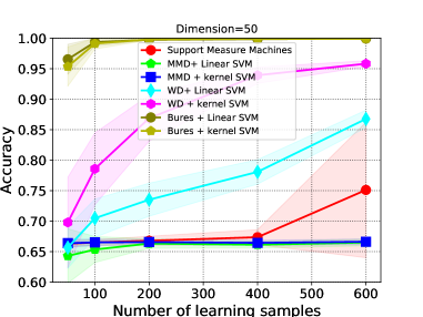
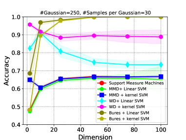
Figure 2: Comparing performances of Support Measure Machines and Wasserstein distance + classifier.

In this section, we have analyzed and compared the performances of Wasserstein distances based embedding for learning to classify distributions. Several toy problems, similar to those described in Section 4.3 have been considered as well as a computer-vision real-world problem.

5.1 Competitors

Before describing the experiments we discuss the algorithms we have compared. We have considered two variants of our approach. The first one embeds the distributions based on $\hat{\rho}_{S}$ by using, unless specified, all distributions available in the training set. The Wasserstein distance is approximated using its entropic regularized version with $\lambda=0.01$ for all problems. Then, we learn either a linear SVM or a Gaussian kernel classifier resulting in two methods dubbed in the sequel as WD+linear and WD+kernel. As discussed in section 3, we can use the closed-form Bures Wassrestein distance when we suppose that the distributions are Gaussian. Assuming that the samples come from a Normal distribution, plugging-in the empirical mean and covariance estimation into the Bures-Wasserstein distance 3 gives us a distance that we can use as an embedding. In the experiments, these approaches are named Bures+linear and Bures+kernel. In the family of integral probability metrics, we used the support measure machines of Muandet et al. , (2012), denoted as SMM. We have considered its non-linear version which used an Gaussian kernel on top of the MMD kernel. In SMM, we have thus two kernel hyperparameters. In order to evaluate the choice of the distance, we have also used the MMD distance in addition to the Wasserstein distance in our framework. These approaches are denoted as MMD+linear and MMD+kernel. Note that we have not reported based on samples-based approaches such as SVM since Muandet et al. , (2012) have already reported that they hardly handle distributions.

Kullback-Leibler divergence can replace the Wasserstein distance in our framework. For instance, we have highlighted that for the problem in Section 4.3, KL-divergence is an $(\epsilon,\gamma)$ good dissimilarity function. We have thus implemented the non-parametric estimation of the KL-divergence based on quadratic programming (Nguyen et al. ,, 2010, 2007). After few experiments on the toy problems, we finally decided to not report performance of the KL-divergence based approach due to its poor computational scalability as illustred in the supplementary material.

5.2 Simulated problem

These problems aim at studying the performances of our models in controlled setting. The toy problem corresponds to the one described in Section 4.3 but with $3$ classes. For all classes, mean of a given distribution follows a normal distribution with mean $\mathbf{m}^{\star}=[1,1]$ and covariance matrix $\sigma\mathbf{I}$ with $\sigma=5$. For class $i$, the covariance matrix of the distribution is defined as $\sigma_{i}\mathbf{I}+u_{i}(\mathbf{I}_{1}+\mathbf{I}_{-1}$) where $\mathbf{I}_{1}$ and $\mathbf{I}_{-1}$ are respectively the super and sub diagonal matrices. The $\{\sigma_{i}\}$ are constant whereas $u_{i}$ follows a uniform distribution depending on the class. We have kept the number of empirical samples per distribution fixed at $N=30$.

For these experiments, we have analyzed the effect of the number of training examples $n$ (which is also the number of templates) and the dimensionality $d$ of the distribution. Approaches are then evaluated on of $2000$ test distributions. $20$ trials have been considered for each $n$ and dimension $d$. We define a trial as follows: we randomly sample the $n$ number of distributions and compute all the embeddings and kernels. For learning, We have performed cross-validation on all parameters of all competitors. This involves all kernel and classifier parameters. Details of all parameters and hyperparameters are given in the appendix.

Left plot in Figure 2 represents the averaged classification accuracy with $N=30$ samples per classes and $d=50$ for increasing number $n$ of empirical training distribution examples. Right plot represents the same but for fixed $n=250$ and increasing dimensionality $d$.

From the left panel, we note that MMD-based distance fails in achieving good performances regardless of how they are employed (kernel or distance based classifier). WDMM performs better than MMD especially as the number of training distrubtions increases. For $n=600$, the difference in performance is almost $30\%$ of accuracy when considering distance-based embeddings. We also remark that the Bures-Wasserstein metric naturally fits to this Normal distribution learning problem and achieves perfect performances for $n\geq 200$.

Right panel shows the Impact of the dimensionality of the problem on the classification performance. We note that again MMD-based approaches do not perform as good as Wasserstein-based ones. Whereas MMD tops below $70\%$, our non-linear WDMM method achieves about $90\%$ of classification rate across a large range of dimensionality.

5.3 Natural scene categorization

Method	Scenes	3DPC	3DPC-CV
SMM	51.58 $\pm$ 2.46	92.79	92.99 $\pm$ 0.99
MMD linear	24.83 $\pm$ 1.22	91.89	91.84 $\pm$ 1.13
MMD kernel	27.02 $\pm$ 4.09	90.54	92.66 $\pm$ 1.02
WD linear	61.58 $\pm$ 1.34	97.30	95.52 $\pm$ 0.89
WD kernel	60.70 $\pm$ 2.49	96.86	94.89 $\pm$ 0.80
BW linear	62.30 $\pm$ 1.32	64.86	63.52 $\pm$ 5.72
BW kernel	62.06 $\pm$ 1.34	70.72	72.20 $\pm$ 1.51

Table 1: Performances of competitors on real-world problems. 3DPC and 3DPC-CV columns report performances on original train/test split and for random splits. Bold denotes best test accuracy and underline show statistically equivalent performance under Wilocoxon signrank test with $p=0.01$.

We have also compared the performance the different approaches on a computer vision problem. For this purpose, we have reproduced the experiments carried out by Muandet et al. , (2012). Their idea is to consider an image of a scene as an histogram of codewords, where the codewords have been obtained by k-means clustering of $128$-dim SIFT vector and thus to use this histogram as a discrete probability distribution for classifying the images. Details of the feature extraction pipeline can be found in the paper Muandet et al. , (2012). The only difference our experimental set-up is that we have used an enriched version of the dataset they used. Similarly, we have used $100$ images per class for training and the rest for testing. Again, all hyperparameters of all competing methods have been selected by cross-validation.

The averaged results over $10$ trials are presented in Table 1. Again, the plot illustrates the benefit of Wasserstein-distance based approaches (through fully non-parametric distance estimation or through the estimated Bures-Wasserstein metric) compared to MMD based methods. We believe that the gain in performance for non-parametric methods is due to the ability of the Wasserstein distance to match samples of one distribution to only few samples of the other distribution. By doing so, we believe that it is able to capture in an elegant way complex interaction between samples of distributions.

5.4 3D point cloud classification

3D point cloud can be considered as samples from a distribution. As such, a natural tool for classifying them is to used metrics or kernels on distributions. In this experiment, we have benchmarked all competitors on a subset of the ModelNet10 dataset . Among the 10 classes in that dataset, we have extracted the night stand, desk and bathtub classes which respectively have $400$, $400$ and $212$ training examples and $172$,$172$ and $100$ test examples. Experiments and model selection have been run as in previous experiments. In Table 1, we report results based on original train and test sets and results using $50-50$ random splits and resamplings. Again, we highlight the benefit of using the Wasserstein distance as an embedding and contrarily to other experiments, the Bures-Wasserstein metric yields to poor performance as the object point clouds hardly fit a Normal distribution leading thus to model misspecification.

6 Conclusion

This paper introduces a method for learning to discriminate probability distributions based on dissimilarity functions. The algorithm consists in embedding the distributions into a space of dissimilarity to some template distributions and to learn a linear decision function in that space. From a theoretical point of view, when considering population distributions, our framework is an extension of the one of Balcan et al. , (2008). But we provide a theoretical analysis showing that for embeddings based on empirical distributions, given enough samples, we can still learn a linear decision functions with low error with high-probability with empirical Wasserstein distance. The experimental results illustrate the benefits of using empirical dissimilarity on distributions on toy problems and real-world data.

Futur works will be oriented toward analyzing a more general class of regularized optimal transport divergence, such as the Sinkhorn divergence Genevay et al. , (2017) in the context of Wasserstein distance measure machines. Also, we will consider extensions of this framework to regression problems, for which a direct application is not immediate.

References

- Arjovsky et al. , (2017) Arjovsky, Martin, Chintala, Sumit, & Bottou, Léon. 2017. Wasserstein Generative Adversarial Networks. Pages 214–223 of: ICML.
- Balcan et al. , (2008) Balcan, Maria-Florina, Blum, Avrim, & Srebro, Nathan. 2008. A theory of learning with similarity functions. Machine Learning, 72(1-2), 89–112.
- Bhattacharyya, (1943) Bhattacharyya, Anil. 1943. On a measure of divergence between two statistical populations defined by their probability distributions. Bull. Calcutta Math. Soc., 35, 99–109.
- Breiman, (2001) Breiman, Leo. 2001. Random forests. Machine learning, 45(1), 5–32.
- Bures, (1969) Bures, Donald. 1969. An extension of Kakutani’s theorem on infinite product measures to the tensor product of semifinite -algebras. Transactions of the American Mathematical Society, 135, 199–212.
- Courty et al. , (2017) Courty, Nicolas, Flamary, Rémi, Tuia, Devis, & Rakotomamonjy, Alain. 2017. Optimal transport for domain adaptation. IEEE Transactions on Pattern Analysis and Machine Intelligence.
- Dietterich et al. , (1997) Dietterich, Thomas G, Lathrop, Richard H, & Lozano-Pérez, Tomás. 1997. Solving the multiple instance problem with axis-parallel rectangles. Artificial intelligence, 89(1-2), 31–71.
- Flaxman et al. , (2015) Flaxman, Seth R, Wang, Yu-Xiang, & Smola, Alexander J. 2015. Who supported Obama in 2012?: Ecological inference through distribution regression. Pages 289–298 of: Proceedings of the 21th ACM SIGKDD International Conference on Knowledge Discovery and Data Mining. ACM.
- Fournier & Guillin, (2015) Fournier, Nicolas, & Guillin, Arnaud. 2015. On the rate of convergence in Wasserstein distance of the empirical measure. Probability Theory and Related Fields, 162(3-4), 707–738.
- Frogner et al. , (2015) Frogner, C., Zhang, C., Mobahi, H., Araya, M., & Poggio, T. 2015. Learning with a Wasserstein Loss. In: NIPS.
- Genevay et al. , (2017) Genevay, A., Peyré, G., & Cuturi, M. 2017. Learning Generative Models with Sinkhorn Divergences. ArXiv e-prints, June.
- Gretton et al. , (2007) Gretton, Arthur, Borgwardt, Karsten M, Rasch, Malte, Schölkopf, Bernhard, & Smola, Alex J. 2007. A kernel method for the two-sample-problem. Pages 513–520 of: Advances in neural information processing systems.
- Gretton et al. , (2012) Gretton, Arthur, Borgwardt, Karsten M, Rasch, Malte J, Schölkopf, Bernhard, & Smola, Alexander. 2012. A kernel two-sample test. Journal of Machine Learning Research, 13(Mar), 723–773.
- Haasdonk & Bahlmann, (2004) Haasdonk, Bernard, & Bahlmann, Claus. 2004. Learning with distance substitution kernels. Pages 220–227 of: Joint Pattern Recognition Symposium. Springer.
- Hein & Bousquet, (2005) Hein, Matthias, & Bousquet, Olivier. 2005. Hilbertian metrics and positive definite kernels on probability measures. Pages 136–143 of: AISTATS.
- Jebara et al. , (2004) Jebara, Tony, Kondor, Risi, & Howard, Andrew. 2004. Probability product kernels. Journal of Machine Learning Research, 5(Jul), 819–844.
- Muandet et al. , (2012) Muandet, Krikamol, Fukumizu, Kenji, Dinuzzo, Francesco, & Schölkopf, Bernhard. 2012. Learning from distributions via support measure machines. Pages 10–18 of: Advances in neural information processing systems.
- Nguyen et al. , (2007) Nguyen, XuanLong, Wainwright, Martin J, & Jordan, Michael I. 2007. Nonparametric estimation of the likelihood ratio and divergence functionals. Pages 2016–2020 of: Information Theory, 2007. ISIT 2007. IEEE International Symposium on. IEEE.
- Nguyen et al. , (2010) Nguyen, XuanLong, Wainwright, Martin J, & Jordan, Michael I. 2010. Estimating divergence functionals and the likelihood ratio by convex risk minimization. IEEE Transactions on Information Theory, 56(11), 5847–5861.
- Ntampaka et al. , (2015) Ntampaka, Michelle, Trac, Hy, Sutherland, Dougal J, Battaglia, Nicholas, Póczos, Barnabás, & Schneider, Jeff. 2015. A machine learning approach for dynamical mass measurements of galaxy clusters. The Astrophysical Journal, 803(2), 50.
- Póczos et al. , (2012) Póczos, Barnabás, Xiong, Liang, Sutherland, Dougal J, & Schneider, Jeff. 2012. Nonparametric kernel estimators for image classification. Pages 2989–2996 of: Computer Vision and Pattern Recognition (CVPR), 2012 IEEE Conference on. IEEE.
- Póczos et al. , (2013) Póczos, Barnabás, Singh, Aarti, Rinaldo, Alessandro, & Wasserman, Larry A. 2013. Distribution-Free Distribution Regression. Pages 507–515 of: AISTATS.
- Ramdas et al. , (2015) Ramdas, Aaditya, Reddi, Sashank Jakkam, Póczos, Barnabás, Singh, Aarti, & Wasserman, Larry A. 2015. On the decreasing power of kernel and distance based nonparametric hypothesis tests in high dimensions. Pages 3571–3577 of: AAAI.
- Schölkopf & Smola, (2002) Schölkopf, Bernhard, & Smola, Alexander J. 2002. Learning with kernels: support vector machines, regularization, optimization, and beyond. MIT press.
- Sriperumbudur et al. , (2010) Sriperumbudur, Bharath K, Fukumizu, Kenji, Gretton, Arthur, Schölkopf, Bernhard, & Lanckriet, Gert RG. 2010. Non-parametric estimation of integral probability metrics. Pages 1428–1432 of: Information Theory Proceedings (ISIT), 2010 IEEE International Symposium on. IEEE.
- Sutherland et al. , (2012) Sutherland, Dougal J, Xiong, Liang, Póczos, Barnabás, & Schneider, Jeff. 2012. Kernels on sample sets via nonparametric divergence estimates. arXiv preprint arXiv:1202.0302.
- Villani, (2009) Villani, C. 2009. Optimal transport: old and new. Grund. der mathematischen Wissenschaften. Springer.
- Weed & Bach, (2017) Weed, Jonathan, & Bach, Francis. 2017. Sharp asymptotic and finite-sample rates of convergence of empirical measures in Wasserstein distance. arXiv preprint arXiv:1707.00087.