Inorbit Performance of the Hard X-ray Telescope (HXT) on board the Hitomi (ASTRO-H) satellite

Abstract

Hitomi (ASTRO-H) carries two Hard X-ray Telescopes (HXTs) that can focus X-rays up to 80 keV. Combined with the Hard X-ray Imagers (HXIs) that detect the focused X-rays, imaging spectroscopy in the high-energy band from 5 keV to 80 keV is made possible. We studied characteristics of HXTs after the launch such as the encircled energy function (EEF) and the effective area using the data of a Crab observation. The half power diameters (HPDs) in the 5–80 keV band evaluated from the EEFs are 1.59 arcmin for HXT-1 and 1.65 arcmin for HXT-2. Those are consistent with the HPDs measured with ground experiments when uncertainties are taken into account. We can conclude that there is no significant change in the characteristics of the HXTs before and after the launch. The off-axis angle of the aim point from the optical axis is evaluated to be less than 0.5 arcmin for both HXT-1 and HXT-2. The best-fit parameters for the Crab spectrum obtained with the HXT-HXI system are consistent with the canonical values.

*Hironori Matsumoto, matumoto@ess.sci.osaka-u.ac.jp

1 Introduction

Hitomi (ASTRO-H) 1, developed based on an international collaboration led by ISAS/JAXA in Japan, was launched on February 17, 2016. Hitomi carries two types of X-ray telescopes; one is the Soft X-ray Telescope (SXT) 2 that focuses X-rays below 10 keV, and the other is the Hard X-ray Telescope (HXT) 3 that can focus X-rays up to 80 keV. The HXT adopts a conical approximation to the Wolter-I optics design with a focal length of 12 m. Thin foils of aluminum with a thickness of 0.2 mm and a height of 200 mm are used as reflector substrates. The radius of the innermost reflector is 60 mm, and that of the outermost reflector is 225 mm. The surface of the foils is covered with a multilayer of platinum and carbon to reflect hard X-rays by Bragg reflection. The total number of nesting shells is 213, and the aperture is divided into three segments along the azimuthal direction. Since the HXT utilizes two-stage reflection, the total number of reflectors is $213\times 3\times 2=1278$. There are 14 kinds of multilayers that are applied to the HXT, and the details of the design is described in Awaki et al. (2014) 3 and Tamura et al. (2018) 4. There are two HXTs on board Hitomi, and they are called HXT-1 and HXT-2. The Hard X-ray Imager (HXI) 5 is placed at the focal point of each HXT, and HXI-1 and HXI-2 are combined with HXT-1 and HXT-2, respectively. Basic parameters of the HXT are summarized in Table 1.

Table 1: Basic Parameters of the HXT.

Number of telescopes	2 (HXT-1 & HXT-2)
Focal length	12 m
Substrate	aluminum
Substrate thickness	0.2 mm
Substrate height	200 mm
Coated multilayer	platinum and carbon
Number of nesting shells	213
Radius of innermost reflector	60 mm
Radius of outermost reflector	225 mm
Geometrical area	968 cm2/telescope

The HXTs were characterized with ground experiments mainly done at the beam line BL20B2 of the synchrotron facility SPring-8 6. To analyze an X-ray spectrum of a celestial object obtained with the HXT-HXI system, an Ancillary Response File (ARF) that describes the specifics of the response of the HXT such as an effective area for the object and a Redistribution Matrix File (RMF) that describes the response of the HXI are needed. The ARF is calculated by a raytrace program 7 based on the results of the ground experiments. If the characteristics of the HXTs change after the launch, the changes have to be incorporated into the ARF calculation. For example, if the shape of the thin foils change due to the release of gravitational stress in orbit, the angular resolution and the effective area may change. Although Hitomi experienced an attitude control anomaly and was lost a month after the launch, the HXT-HXI system was able to observe several objects in the first month. In this paper, we studied the inorbit performance of the HXTs using data from a Crab observation, and compared the results with those obtained from the ground experiments to see if any change occurred in the characteristics of the HXTs after the launch. Uncertainties are given at the $1~{}\sigma$ confidence level unless otherwise stated in this work.

2 Operation

After the launch of Hitomi 1 on February 17, 2016, HXI-1 5 began to operate from March 12, 2016 when Hitomi targeted the high-mass X-ray binary IGR J$16318-4848$. The target was, however, outside the field of view of the HXI-1. The HXI-2 was turned on on March 14 during the course of maneuver from IGR J$16318-4848$ to the neutron star RX J$1856.5-3754$ which is one of the X-ray dim isolated neutron stars with strong magnetic fields 8. The neutron star is known to exhibit predominantly soft X-rays below 2 keV9 and was observed for the calibration of the SXT2, Soft X-ray Spectrometer (SXS)10, and Soft X-ray Imager (SXI)11 in the soft energy band. The X-rays from RX J$1856.5-3754$ were too soft to be detected with the HXT-HXI system. Hitomi observed the pulsar wind nebula G $21.5-0.9$ after RX J$1856.5-3754$ on March 19, 2016. Hard X-rays from this object were the first light for the HXT-HXI system. Then Hitomi observed RX J$1856.5-3754$ again on March 22, 2016, and the Crab nebula was observed on March 25, 2016. The exposure time of the Crab observation was about 8 ks. The Crab nebula was the 2nd object that the HXT-HXI system detected hard X-ray photons at its aim point.

Thus G $21.5-0.9$ and the Crab nebula can be used to address the inflight performance of the HXT. The hard X-ray emission from G $21.5-0.9$ is dominated by the pulsar wind nebula and is spatially extended12. Thus G $21.5-0.9$ is not an ideal target for characterizing the performance of the HXT. The hard X-ray emission of the Crab nebula is also known to be spatially extended. However, the pulsation from the Crab pulsar was successfully detected with the HXI5, while the pulsations from G $21.5-0.9$ were not detected12. Using the pulse information of the Crab pulsar, we can construct X-ray images of the pulsar point source as described below, and those images can be used to address the performance of the HXT. Thus we concentrate on the Crab data in this paper. The observation log of the Crab nebula is summarized in Table 2.

Table 2: Observation log of the Crab nebula.

Sequence Number	Observation start (UT)	Exposure (ks)	count rate (cts s-1)
100044010	2016/3/25 12:37:19	8.01	397.9 (HXI-1), 403.0 (HXI-2)

3 Encircled Energy Function

We used the cleaned event data of the Crab nebula with the standard screening for the post-pipeline data reduction13. The sequence ID is 100044010, and the processing script version of the data is 01.01.003.003. The barycentric correction was applied where the target position was the Crab pulsar position of $(\alpha,\delta)_{\rm J2000}=(83.6332208,22.0144614)$14. The image of HXI-1 using all cleaned data is shown in Fig. 1. The X-ray image consists of the Crab pulsar that is a point source and the nebula around the pulsar that is spatially extended. In order to study the encircled energy function (EEF) of HXTs, we need an X-ray image of a point source. An X-ray image of the Crab pulsar excluding the nebula emission was made as described below.

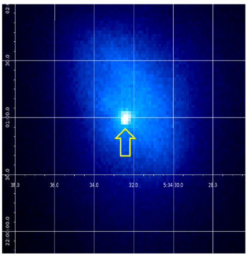
Figure 1: X-ray image of the Crab nebula in an energy band of 5 – 80 keV obtained with the HXI-1. The position of the Crab pulsar is shown with an arrow.

It is well known that the Crab pulsar exhibits X-ray pulsations with a period of $\sim$33 ms. The pulsations have a double peak structure. The larger pulse is called P1 and the smaller one is called P215, 16. Since the HXI has a time resolution of $25.6~{}\mu{\rm s}$5, the pulsations were successfully detected by the HXI, and X-ray images during the pulse P1 (phases 0.0–0.05 and 0.85–1.0) and during an off-pulse phase (phase 0.45–0.85; hereafter OFF1) were obtained. If we subtract the OFF1 image from the P1 image, we can obtain the X-ray image of the Crab pulsar. However, since the count rate is large, a dead time fraction has to be taken into account in the subtraction process. The method used for estimating the dead time fraction is described in Appendix A.

After obtaining the dead time fraction of each pulse phase, X-ray images of the Crab pulsar was obtained by applying a dead time correction. For example, for the HXI-1, the exposure time of the OFF1 image was $3.441\times 10^{3}$ s, and the real exposure time was $3.441\times 10^{3}~{}{\rm s}\times(1-0.2210)=2.681\times 10^{3}~{}{\rm s}$. The exposure time of the P1 image was $1.7205\times 10^{3}$ s, and the real exposure time was $1.7205\times 10^{3}~{}{\rm s}\times(1-0.2571)=1.278\times 10^{3}~{}{\rm s}$. Then the Crab pulsar image of HXI-1 was obtained by (P1 image) - (OFF1 image) $\times(1.278\times 10^{3}~{}{\rm s}/2.681\times 10^{3}~{}{\rm s})$. The image of HXI-2 was obtained in the same manner. The X-ray images in the 5 – 80 keV band thus obtained are shown in Fig. 2.

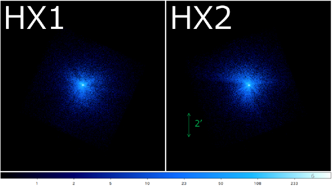
Figure 2: X-ray image of the Crab pulsar in the energy band of 5 – 80 keV obtained with HXI-1 (left) and HXI-2 (right).

The EEFs constructed from these images are shown in Fig. 3; in this case, the EEF is defined as the ratio of the number of photons detected within a circular region with a radius $r$ to those within a circle with a radius of 4 arcmin. The center of the circular regions coincides with the position of the Crab pulsar. Since the field of view of HXI is 9 arcmin, the outermost radius of the EEF is limited to 4 arcmin. The average number of photons per pixel in the field of view but outside the circle of 4 arcmin radius was subtracted from the images as background. The EEFs obtained by the ground experiments done at SPring-8 6 are also plotted in Fig. 3; while the EEFs in Mori et al. (2018) 6 are normalized at 6.2 arcmin, the EEFs here are recalculated with the same procedure as that used for the Crab image and are normalized at 4 arcmin. The half power diameter (HPD) is defined as the diameter where the EEF equals to 0.5, and the HPDs are shown in Table 3. Considering the uncertainty of the dead time fraction, the uncertainty on the inorbit HPDs is $\sim 0.1$ arcmin. The HPDs from the ground experiments also have an uncertainty of $\sim 0.1$ arcmin 6. The inorbit HPDs and those from the ground experiments in Table 3 are consistent with each other when the uncertainties are taken into consideration. Thus, the image quality in terms of the HPD does not show a significant change between ground and in-orbit measurements. Fig 3 suggests, however, that the inorbit EEFs may be systematically narrower than those from the ground experiments. The release of the gravitational stress may cause the slight contraction of the EEFs. We can conclude that the performance of HXTs did not change significantly before and after the launch of Hitomi. The requirement on the HPD is 1.7 arcmin at 30 keV 3 using the EEF normalized at 6 arcmin, and the requirement using the EEF normalized at 4 arcmin corresponds to $\sim 1.6$ arcmin. To see inorbit HPDs at 30 keV, we examined the EEFs in the 25–35 keV band and they are shown in Fig. 4. The HPDs obtained from those EEFs are also included in Table 3. Thus the HPD of HXT-1 in the 25–35 keV band satisfies the requirement. Although the HPD of HXT-2 is slightly larger than the requirement, it is consistent with the requirement within the uncertainties in the measurement.

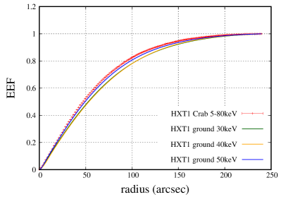
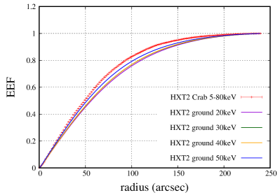
Figure 3: Encircled Energy Functions (EEFs) in the 5 – 80 keV band of HXT-1 (left) and HXT-2 (right) normalized at 4 arcmin are shown with red data points. EEFs obtained with ground experiments at 20 keV (purple), 30 keV (green), 40 keV (orange) and 50 keV (blue) are also plotted. Error bars on the data are given at the $1~{}\sigma$ confidence level.

Table 3: Half Power Diameters

	HXT-1	HXT-2
	(arcmin)	(arcmin)
Inorbit 5–80 keV	1.59	1.65
25 – 35 keV	1.59	1.77
Ground 20 keV	—	1.89
30 keV	1.77	1.84
40 keV	1.79	1.84
50 keV	1.64	1.73

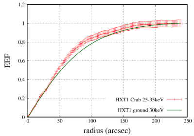
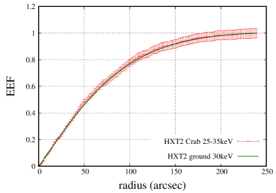
Figure 4: EEFs in the 25 – 35 keV band of HXT-1 (left) and HXT-2 (right) normalized at 4 arcmin are shown with red data points. EEFs obtained with ground experiments at 30 keV (green) is also plotted. Error bars on the data are given at the $1~{}\sigma$ confidence level.

4 Off-axis angle of the aim point from the HXT optical axis

The direction of the optical axis is defined as the direction of the telescope at which the effective area is maximized. It is required to observe an X-ray source with various offset angles to determine the direction of the optical axis. However, the Crab nebula was observed at the aim point of the HXI, and we have no off-axis observations. It is impossible to determine the direction of the optical axis precisely. However, we can estimate the off-axis angle of the aim point from the HXT optical axis by comparing the spectrum of the Crab nebula with model predictions calculated by the raytracing program 7 with different off-axis angles.

The cleaned data of the Crab nebula of the processing script version 01.01.003.003 were used. We extracted the spectrum of the Crab nebula including all pulse phases from a circle with a radius of 4 arcmin centered at the position of the Crab pulsar. The dead-time fraction was estimated using the pseudo events. As is described in the appendix A, this method gives only a rough estimation of the dead-time fraction. However, this estimation is enough for the study in this section, since the dead-time fraction is considered to have no energy dependence and affects only the overall normalization of an X-ray spectrum. The background spectrum for each sensor was obtained from blank sky observations.

A power-law model modified by the photoelectric absorption of an equivalent hydrogen column density of $N_{\rm H}=3\times 10^{21}~{}{\rm cm}^{-2}$ 17 was fitted to the spectrum with various ARFs; the ARFs were created by assuming that the off-axis angle of the Crab pulsar from the optical axis is 0.0 arcmin, 0.5 arcmin, 1.0 arcmin, and 2.0 arcmin. In the ARF calculation, auxiliary transmission files ah_hx[12]_auxtran_20140101v001.fits were used. Though the raytrace program is based on the results of the ground experiments, there are small differences (8 % at most) between the effective area measured at the ground experiments and the area predicted by the raytrace simulation. The cause of the difference is not well understood, and the auxiliary transmission files compensate the differences by using arbitrary scaling factors. The HXI-1 spectra with the best-fit models are shown in Fig. 5. The best-fit parameters and the $\chi^{2}$ values are listed in Table 4. Note that the normalizations in this Table are affected by the rough estimation of the dead-time fraction. It is clear that an off-axis angle of 1.0 arcmin or more cannot explain the spectrum at the high energy side and the $\chi^{2}/d.o.f.$ value becomes large as the off-axis angle increases. This is because the vignetting function becomes narrower as photon energy increases 3, 6. We can conclude that the off-axis angle of the aim point from the optical axis is less than 0.5 arcmin.

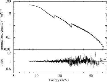
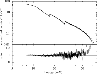
Figure 5: HXT-1 spectrum of the Crab nebula in the 8 – 80 keV band is fitted by a power-law model using ARFs assuming the off-axis angle of the Crab pulsar from the optical axis is 0.0 arcmin (top left), 0.5 arcmin (top right), 1.0 arcmin (bottom left), and 2.0 arcmin (bottom right). The lower panels show the ratio between the data and the best-fit model. Error bars on the data are given at the $1~{}\sigma$ confidence level.

Table 4: Spectrum fit of the Crab nebula with ARFs assuming various off-axis angles.

	Off-axis angle for ARF of HXT-1
	on-axis	0.5 arcmin	1.0 arcmin	2.0 arcmin
Photon index	$2.114^{+0.004}_{-0.004}$	$2.111^{+0.004}_{-0.004}$	$2.093^{+0.004}_{-0.004}$	$2.045$
Normalization	$10.39^{+0.09}_{-0.09}$	$10.50^{+0.10}_{-0.09}$	$10.52^{+0.10}_{-0.09}$	$10.97$
Flux (2–10 keV)	$2.27\times 10^{-8}$	$2.30\times 10^{-8}$	$2.36\times 10^{-8}$	$2.65\times 10^{-8}$
$\chi^{2}/d.o.f.$	$354/360$	$363/360$	$397/360$	$630/360$

	Off-axis angle for ARF of HXT-2
	on-axis	0.5 arcmin	1.0 arcmin	2.0 arcmin
Photon index	$2.112^{+0.004}_{-0.004}$	$2.111^{+0.003}_{-0.004}$	$2.095^{+0.004}_{-0.004}$	$2.053$
Normalization	$9.99^{+0.09}_{-0.09}$	$10.12^{+0.09}_{-0.09}$	$10.19^{+0.09}_{-0.09}$	$10.87$
Flux (2–10 keV)	$2.18\times 10^{-8}$	$2.21\times 10^{-8}$	$2.28\times 10^{-8}$	$2.59\times 10^{-8}$
$\chi^{2}/d.o.f.$	$402/365$	$416/365$	$459/365$	$825/365$

Uncertainties are given at the 90 % confidence level.
Flux values are given in erg s^-1 cm^-2.
Normalizations are defined as the photon number flux at 1 keV.

5 Inflight Performance and Raytrace

After establishing the off-axis angle of the aim point from the optical axis is small, we can make the reasonable assumption that the Crab pulsar was observed at the on-axis position. Then the power-law model was fitted to the spectra of the Crab nebula of HXI-1 and HXI-2 simultaneously. In this analysis, the cleaned data of the Crab nebula of the processing script version 01.01.003.003 were reprocessed to be equivalent to those of 02.01.004.004. The dead-time correction described in the appendix A was applied. The column density was fixed to $N_{\rm H}=3\times 10^{21}~{}{\rm cm}^{-2}$. The photon indices for both sensors were set to a common value, while the normalizations for both sensors were varied separately. The best-fit $\chi^{2}/d.o.f.$ is $738/679$. The photon index is $2.122\pm 0.003$, and the normalization, which is defined as the photon number flux at 1 keV, is $10.70\pm 0.07$ for HXI-1 and $10.59\pm 0.07$ for HXI-2, where the uncertainties are given at the 90 % confidence level. These values are consistent with the “canonical” values of the photon index $2.10\pm 0.03$ and the normalization $9.7\pm 1.0$ in Toor and Seward (1984) 18. The difference of the normalizations of HXI-1 and HXI-2 is $\sim 1$ %. The unabsorbed energy flux in the 3–50 keV band calculated from the normalization is $3.59\times 10^{-8}~{}{\rm erg~{}cm^{-2}~{}s^{-1}}$ for HXI-1 and $3.55\times 10^{-8}~{}{\rm erg~{}cm^{-2}~{}s^{-1}}$ for HXI-2. These values are $\sim 5\%$ larger than the flux of $3.37\times 10^{-8}~{}{\rm erg~{}cm^{-2}~{}s^{-1}}$ measured with NuSTAR 19.

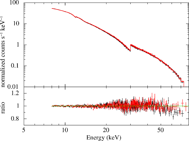
Figure 6: Spectra of the Crab nebula in the 8 – 80 keV band of HXI-1 (black) and HXI-2 (red) together with the best-fit power-law model using the on-axis ARFs. The lower panels show the ratio between the data and the best-fit model. Error bars on the data are given at the $1~{}\sigma$ confidence level.

Fig. 7 shows the EEF of the Crab pulsar in the 5–80 keV band generated in section 3 together with those predicted by the raytracing program. The bottom panel shows the ratio between them as dotted lines. The ratios between the EEFs from the ground experiments and from the raytrace calculations are also plotted as dashed lines. The deviation between the raytrace EEFs and the Crab EEF is less than 10 % except for the central region within a radius 0.2 arcmin. We should note that if we extract an HXI spectrum from a circular region with a small radius, the effective area for the spectrum calculated using the raytrace program has a systematic uncertainty.

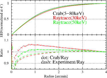
Figure 7: EEF of the Crab pulsar in the 5–80 keV band (black) is compared with those predicted by the raytrace program at 30 keV (red) and 50 keV (green) in the top panel: HXT-1 (left) and HXT-2 (right). Ratios between them are plotted with the dotted line in the bottom panel, while ratios of the EEFs obtained by the ground experiment to the raytrace EEFs are shown as the dashed line. Error bars on the data are given at the $1~{}\sigma$ confidence level.

6 Summary

The X-ray image of the Crab pulsar point source for the HXT-HXI system was obtained by subtracting the Crab image during the off-pulse (OFF1) phase from that during the on-pulse (P1) phase. In the subtraction process, the dead time fraction was taken into account. The EEF normalized at a radius of 4 arcmin was constructed from the image. The HPD was estimated from the EEF, and the HPDs in the 5–80 keV band are 1.59 arcmin for HXT-1 and 1.65 arcmin for HXT-2. These HPDs are consistent with those obtained from the ground experiments within the uncertainty, and this suggests that there is no significant change in the characteristics of HXTs before and after the launch of Hitomi. We estimate that the off-axis angle of the aim point from the direction of the optical axis is less than 0.5 arcmin for both HXT-1 and HXT-2 as determined by the model fitting of the spectrum of the Crab nebula using ARFs assuming various off-axis angles. The best-fit parameters for the Crab spectrum are consistent with the canonical values of Toor & Seward[18]. The deviation between the inorbit EEF and those calculated by the raytrace program is less than 10 % except for the region with a radius smaller than 0.2 arcmin.

Appendix A Evaluation of the Dead Time Fractions

The HXI has pseudo events that are randomly distributed with a mean frequency of 2 Hz. The number of pseudo events gives an estimate of the exposure time after the dead time loss. Since the total exposure time is 8 ks and then the exposure time of each pulse phase is only a few ks, however, the Poisson fluctuation of the pseudo events dominates the uncertainty in the estimation of the dead time fraction of each pulse phase. For example, the dead time fraction of HXI-1 during the pulse P1 phase was estimated to be 24.4 % by using the pseudo events, while that during the off-pulse phase was to be 24.5 %. Of course the former should be larger than the latter, and this means that the uncertainty in the dead time fraction estimated by the pseudo events was not small. Then we used another method described below to estimate the dead time fractions.

First we estimated a typical dead time of each event. We investigated the distribution of LIVETIME tagged to each event; the livetime of the event is the time interval between the end time of the processing of the previous trigger and the trigger of this event. The distribution should be proportional to $\exp(-nt)$, where $t$ is the livetime and $n$ is the “true” count rate which is the rate that would be recorded if there were no dead time20. The distribution of the live time of all events suggests that $n$ is 726 c s^-1 for HXI-1. The uncertainty of $n$ at the 1 $\sigma$ confidence level is $\sim\ 0.1~{}\%$. If a count rate $m$ recorded after suffering the dead time loss is obtained, we can calculate the dead time per event $\tau$ by $\tau=(1/m)-(1/n)$20. All events are classified on board as a category H, M, or L, where the category H is a normal event, and the categories M and L are the events that coincide with a signal from the active shield counter. The number of events in each category can be found in the HK file as HXI[12]_USER_EVNT_SEL_CNT_[HML]. Using the HK information, the averaged total count rate during the Crab observation recorded with HXI-1 was estimated to be $m=537$ c s^-1. The uncertainty of $m$ at the 1 $\sigma$ confidence level is $\sim\ 0.1~{}\%$. Then the typical dead time $\tau=(1/537)-(1/726)=3.678\times 10^{-4}~{}{\rm s~{}c}^{-1}$.

Next, we evaluated the recorded count rate of each pulse phase. However, the time resolution of the HK information is not sufficient for this purpose. Then we evaluated count rates of the three categories separately and added them. The count rate of the category H can be estimated by just counting the event number in unfiltered event files. However, most of the events of the categories M and L are not included in the event files, since their priority is low and most of them are not kept in the onboard data recorder to save the capacity of the recorder. As for the count rates of the categories M and L, we assumed that they consist of two parts; one is a background constant component which can be measured during the Earth occultation, and the other part comes from events accidentally coincide with the shield events. We assumed that the latter is proportional to the count rate of the category H after subtracting its constant component during the Earth occultation. In summary, we assumed

$$M+L=a\times(H-H_{0})+(M_{0}+L_{0}),$$ (1)

where $a$ is a constant, $H$, $M$, and $L$ denote the count rate of each category respectively, and the subscript $0$ means that those are rates during the Earth occultation. $H_{0}=18.47$ c s^-1 and $M_{0}+L_{0}=15.19$ c s^-1 were obtained for HXI-1 from the HK information. The averaged $H$ and $M+L$ during the Crab observation for HXI-1 were also obtained from the HK information, and $H=536.3$ c s^-1 and $M+L=36.49$ c s^-1. From these values, the constant $a$ for HXI-1 was estimated to be $0.0409$. Then $M+L$ of each pulse phase was estimated from $H$ in each pulse phase, and we added them to obtain $H+M+L$.

Though a measure of the dead time fraction can be obtained by $DT^{\prime}=(H+M+L)\times\tau$, one more correction has to be taken into account. Since LIVETIME is the time interval between H events, it does not reflect the fact that some of the H events accidentally coincide with the shield events and are classified as M or L. The real live time of these accidental M or L events is smaller than their LIVETIME. The accidental event rate corresponds to $a\times(H-H_{0})$ in equation (1). The real dead time fraction was estimated by $DT=1-(1-DT^{\prime})\times(1-f)$, where $f$ is defined as the fraction of the accidental events and is calculated by $f=(a\times(H-H_{0}))/(H+M+L)$. The final results are shown in Table 5. Typical uncertainties on $DT$ at the 1$\sigma$ confidence level is $\sim\ 2~{}\%$. The same procedure was applied for the HXI-2 data, and the results are also listed in Table 5. See the paper on the inflight performance of the HXI21 for more detailed information.

Table 5: Dead time fraction of different pulse phases.

Phase	$H+M+L$ (c s-1)	$DT^{\prime}$	$f$	$DT$
HXI-1 ($\tau=3.678\times 10^{-4}$ s c-1)
0.0–0.05, 0.85 – 1.0 (P1)	619.75	0.2279	0.0372	0.2571
0.05–0.2 (OFF2)	547.99	0.2015	0.0370	0.2315
0.2–0.45 (P2)	612.87	0.2254	0.0372	0.2547
0.45 – 0.85 (OFF1)	518.62	0.1908	0.0368	0.2210
average	566.75	0.2085	0.0370	0.2382
HXI-2 ($\tau=3.744\times 10^{-4}$ s c-1)
0.0–0.05, 0.85 – 1.0 (P1)	662.78	0.2438	0.0332	0.2692
0.05–0.2 (OFF2)	588.25	0.2164	0.0329	0.2425
0.2–0.45 (P2)	654.21	0.2406	0.0332	0.2661
0.45 – 0.85 (OFF1)	557.68	0.2051	0.0328	0.2316
average	607.42	0.2234	0.0330	0.2494

Hironori Matsumoto is a professor at Osaka University. He received his BS, MS, and PhD degrees in physics from Kyoto University in 1993, 1995, 1998, respectively. His research filed is X-ray astronomy including developing instruments. He is a member of SPIE.