Global Convergence of Block Coordinate Descent in Deep Learning

Abstract

Deep learning has aroused extensive attention due to its great empirical success. The efficiency of the block coordinate descent (BCD) methods has been recently demonstrated in deep neural network (DNN) training. However, theoretical studies on their convergence properties are limited due to the highly nonconvex nature of DNN training. In this paper, we aim at providing a general methodology for provable convergence guarantees for this type of methods. In particular, for most of the commonly used DNN training models involving both two- and three-splitting schemes, we establish the global convergence to a critical point at a rate of ${\cal O}(1/k)$, where $k$ is the number of iterations. The results extend to general loss functions which have Lipschitz continuous gradients and deep residual networks (ResNets). Our key development adds several new elements to the Kurdyka-Łojasiewicz inequality framework that enables us to carry out the global convergence analysis of BCD in the general scenario of deep learning.

1 Introduction

Tremendous research activities have been dedicated to deep learning due to its great success in some real-world applications such as image classification in computer vision (Krizhevsky et al., 2012), speech recognition (Hinton et al., 2012; Sainath et al., 2013), statistical machine translation (Devlin et al., 2014), and especially outperforming human in Go games (Silver et al., 2016).

The practical optimization algorithms for training neural networks can be mainly divided into three categories in terms of the amount of first- and second-order information used, namely, gradient-based, (approximate) second-order and gradient-free methods. Gradient-based methods make use of backpropagation (Rumelhart et al., 1986) to compute gradients of network parameters. Stochastic gradient descent (SGD) method proposed by Robbins & Monro (1951) serve as the basis. Much of research endeavour is devoted to adaptive variants of vanilla SGD in recent years, including AdaGrad (Duchi et al., 2011), RMSProp (Tieleman & Hinton, 2012), Adam (Kingma & Ba, 2015) and AMSGrad (Reddi et al., 2018). (Approximate) second-order methods mainly include Newton’s method (LeCun et al., 2012), L-BFGS and conjugate gradient (Le et al., 2011). Despite the great success of these gradient-based methods, they may suffer from the vanishing gradient issue for training deep networks (Goodfellow et al., 2016). As an alternative to overcome this issue, gradient-free methods have been recently adapted to the DNN training, including (but not limited to) block coordinate descent (BCD) methods (Carreira-Perpiñán & Wang, 2014; Zhang & Brand, 2017; Lau et al., 2018; Askari et al., 2018; Gu et al., 2018) and alternating direction method of multipliers (ADMM) (Taylor et al., 2016; Zhang et al., 2016). The main reasons for the surge of attention of these two algorithms are twofold. One reason is that they are gradient-free, and thus are able to deal with non-differentiable nonlinearities and potentially avoid the vanishing gradient issue (Taylor et al., 2016; Zhang & Brand, 2017). As shown in Footnote 2, it is observed that vanilla SGD fails to train a ten-hidden-layer MLPs while BCD still works and achieves a moderate accuracy within a few epochs. The other reason is that BCD and ADMM can be easily implemented in a distributed and parallel manner (Boyd et al., 2011; Mahajan et al., 2017), therefore in favour of distributed/decentralized scenarios.

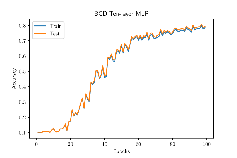
(a) BCD

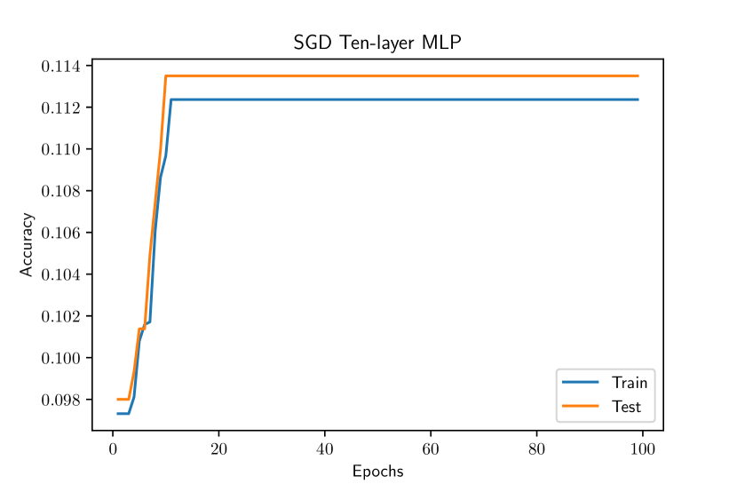
(b) SGD

Figure 1: Comparison of training and test accuracies of BCD and SGD for training ten-hidden-layer MLPs on the MNIST dataset. Refer to Appendix F for details of this experiment.

The BCD methods currently adopted in DNN training run into two categories depending on the specific formulations of the objective functions, namely, the two-splitting formulation and three-splitting formulation (shown in 2.2 and 2.4), respectively. Examples of the two-splitting formulation include Carreira-Perpiñán & Wang (2014); Zhang & Brand (2017); Askari et al. (2018); Gu et al. (2018), whilst Taylor et al. (2016); Lau et al. (2018) adopt the three-splitting formulation. Convergence studies of BCD methods appeared recently in more restricted settings. In Zhang & Brand (2017), a BCD method was suggested to solve the Tikhonov regularized deep neural network training problem using a lifting trick to avoid the computational hurdle imposed by ReLU. Its convergence was established through the framework of Xu & Yin (2013), where the block multiconvexity and differentiability of the unregularized part of the objective function play central roles in the analysis. However, for other commonly used activations such as sigmoid, the convergence analysis of Xu & Yin (2013) cannot be directly applied since the block multiconvexity may be violated. Askari et al. (2018) and Gu et al. (2018) extended the lifting trick introduced by Zhang & Brand (2017) to deal with a class of strictly increasing and invertible activations, and then adapted BCD methods to solve the lifted DNN training models. However, no convergence guarantee was provided in both Askari et al. (2018) and Gu et al. (2018). Following the similar lifting trick as in Zhang & Brand (2017), Lau et al. (2018) proposed a proximal BCD based on the three-splitting formulation of the regularized DNN training problem with ReLU activation. The global convergence was also established through the analysis framework of Xu & Yin (2013). However, similar convergence results for other commonly used activation functions are still lacking.

In this paper, we aim to fill these gaps. Our main contribution is to provide a general methodology to establish the global convergence of these BCD methods in the common DNN training settings, without requiring the block multiconvexity and differentiability assumptions as in Xu & Yin (2013). Instead, our key assumption is the Lipschitz continuity of the activation on any bounded set (see 1(b)). Specifically, Theorem 1 establishes the global convergence to a critical point at an $\mathcal{O}(1/k)$ rate of the BCD methods using the proximal strategy, while extensions to the prox-linear strategy for general losses are provided in Theorem 2 and to residual networks (ResNets) are shown in Theorem 3. Our assumptions are applicable to most cases appeared in the literature. Specifically in Theorem 1, if the loss function, activations, and convex regularizers are lower semicontinuous and either real-analytic (see Definition 1) or semialgebraic (see Definition 2), and the activations are Lipschitz continuous on any bounded set, then BCD converges to a critical point at an $\mathcal{O}(1/k)$ rate starting from any finite initialization, where $k$ is the number of iterations. Note that these assumptions are satisfied by most commonly used DNN training models, where (a) the loss function can be any of the squared, logistic, hinge, exponential or cross-entropy losses, (b) the activation function can be any of ReLU, leaky ReLU, sigmoid, tanh, linear, polynomial, or softplus functions, and (c) the regularizer can be any of the squared $\ell_{2}$ norm, squared Frobenius norm, the elementwise $1$-norm, or the sum of squared Frobenuis norm and elementwise $1$-norm (say, in the vector case, the elastic net by Zou & Hastie, 2005), or the indicator function of the nonnegative closed half space or a closed interval (see Proposition 1).

Our analysis is based on the Kurdyka-Łojasiewicz (KŁ) inequality (Łojasiewicz, 1993; Kurdyka, 1998) framework formulated in Attouch et al. (2013). However there are several different treatments compared to the state-of-the-art work (Xu & Yin, 2013) that enables us to achieve the general convergence guarantee aforementioned. According to Attouch et al. (2013, Theorem 2.9), the sufficient descent, relative error and continuity conditions, together with the KŁ assumption yield the global convergence of a nonconvex algorithm. In order to obtain the sufficient descent condition, we exploit the proximal strategy for all non-strongly convex subproblems (see Algorithm 2 and Lemma 1), without requiring the block multiconvexity assumption used in Xu & Yin (2013, Lemma 2.6). In order to establish the relative error condition, we use the Lipschitz continuity of the activation functions and perform some careful treatments on the specific updates of the BCD methods (see Lemma 2), without requiring the (locally) Lipschitz differentiability of the unregularized part as used in Xu & Yin (2013, Lemma 2.6). The continuity condition is established via the lower semicontinuity assumptions of the loss, activations and regularizers. The treatments of this paper are of their own value to the optimization community. The detailed comparisons between this paper and the existing literature can be found in Section 4.

The rest of this paper is organized as follows. Section 2 describes the BCD methods when adapted to the splitting formulations of DNN training problems. Section 3 establishes their global convergence results, followed by some extensions. Section 4 illustrates the key ideas of proof with some discussions. We conclude this paper in Section 5.

2 DNN training via BCD

In this section, we describe the specific forms of BCD involving both two- and three-splitting formulations.

2.1 DNN training with variable splitting

Consider $N$-layer feedforward neural networks with $N-1$ hidden layers of the neural networks. Particularly, let $d_{i}\in\mathbb{N}$ be the number of hidden units in the $i$-th hidden layer for $i=1,\ldots,N-1$. Let $d_{0}$ and $d_{N}$ be the number of units of input and output layers, respectively. Let $\bm{W}_{i}\in\mathbb{R}^{d_{i}\times d_{i-1}}$ be the weight matrix between the $(i-1)$-th layer and the $i$-th layer for any $i=1,\ldots N$. Let ${\cal Z}:=\{(\bm{x}_{j},\bm{y}_{j})\}_{j=1}^{n}{\subset\mathbb{R}^{d_{0}}\times\mathbb{R}^{d_{N}}}$ be $n$ samples, where $\bm{y}_{j}$’s are the one-hot vectors of labels. Denote $\mathcal{W}:=\{\bm{W}_{i}\}_{i=1}^{N}$, $\bm{X}:=(\bm{x}_{1},\bm{x}_{2},\ldots,\bm{x}_{n})\in\mathbb{R}^{d_{0}\times n}$ and $\bm{Y}:=(\bm{y}_{1},\bm{y}_{2},\ldots,\bm{y}_{n})\in\mathbb{R}^{d_{N}\times n}$. With the help of these notations, the DNN training problem can be formulated as the following empirical risk minimization:

$$\min_{\mathcal{W}}\mathcal{R}_{n}(\Phi(\bm{X};\mathcal{W}),\bm{Y}),$$ (2.1)

where $\mathcal{R}_{n}\left(\Phi(\bm{X};\mathcal{W}),\bm{Y}\right)~{}:=~{}\frac{1}{n}\sum_{j=1}^{n}\ell\left(\Phi(\bm{x}_{j};\mathcal{W}),\bm{y}_{j}\right)$, $\ell:\mathbb{R}^{d_{N}}\times\mathbb{R}^{d_{N}}\rightarrow\mathbb{R}_{+}\cup\{0\}$ is some loss function, $\Phi(\bm{x}_{j};\mathcal{W})=\sigma_{N}(\bm{W}_{N}\sigma_{N-1}(\bm{W}_{N-1}\cdots\bm{W}_{2}\sigma_{1}(\bm{W}_{1}\bm{x}_{j}))$ is the neural network model with $N$ layers and weights $\mathcal{W}$ and $\sigma_{i}$ is the activation function of the $i$-th layer (generally, $\sigma_{N}\equiv\mathrm{Id}$, i.e., the identity function) and $\mathcal{R}_{n}$ is called the empirical risk (also known as the training loss).

Note that the DNN training model (2.1) is highly nonconvex as the variables are coupled via the deep neural network architecture, which brings many challenges for the design of efficient training algorithms and also its theoretical analysis. To make Problem (2.1) more computationally tractable, variable splitting is one of the most commonly used ways (Taylor et al., 2016; Zhang & Brand, 2017; Askari et al., 2018; Gu et al., 2018; Lau et al., 2018). The main idea of variable splitting is to transform a complicated problem (where the variables are coupled highly nonlinearly) into a relatively simpler one (where the variables are coupled much looser) via introducing some additional variables.

2.1.1 Two-splitting formulation.

Considering general deep neural network architectures, the DNN training problem can be naturally formulated as the following model (called two-splitting formulation):

$$\vspace*{-2mm}\min_{\mathcal{W},\mathcal{V}}\mathcal{L}_{0}\left(\mathcal{W},\mathcal{V}\right) :=\mathcal{R}_{n}(\bm{V}_{N};\bm{Y})+\sum_{i=1}^{N}r_{i}(\bm{W}_{i})+\sum_{i=1}^{N}s_{i}(\bm{V}_{i})$$

$$\text{subject to}\quad\bm{V}_{i} =\sigma_{i}(\bm{W}_{i}\bm{V}_{i-1}),\quad i=1,\ldots,N,$$ (2.2)

where $\mathcal{R}_{n}(\bm{V}_{N};\bm{Y}):=\frac{1}{n}\sum_{j=1}^{n}\ell\left((\bm{V}_{N})_{:j},\bm{y}_{j}\right)$ denotes the empirical risk, $\mathcal{V}:=\{\bm{V}_{i}\}_{i=1}^{N}$, $(\bm{V}_{N})_{:j}$ is the $j$-th column of $\bm{V}_{N}$. In addition, $r_{i}$ and $s_{i}$ are extended-real-valued, nonnegative functions revealing the priors of the weight variable $\bm{W}_{i}$ and the state variable $\bm{V}_{i}$ (or the constraints on $\bm{W}_{i}$ and $\bm{V}_{i}$) for each $i=1,\ldots N$, and define $\bm{V}_{0}:=\bm{X}$. In order to solve the two-splitting formulation (2.2), the following alternative minimization problem was suggested in the literature:

$$\min_{\mathcal{W},\mathcal{V}}\mathcal{L}\left(\mathcal{W},\mathcal{V}\right):=\mathcal{L}_{0}\left(\mathcal{W},\mathcal{V}\right)+\frac{\gamma}{2}\sum_{i=1}^{N}\|\bm{V}_{i}-\sigma_{i}(\bm{W}_{i}\bm{V}_{i-1})\|_{F}^{2},$$ (2.3)

where $\gamma>0$ is a hyperparameter.

The DNN training model (2.2) can be very general, where: (a) $\ell$ can be the squared, logistic, hinge, cross-entropy or other commonly used loss functions; (b) $\sigma_{i}$ can be ReLU, leaky ReLU, sigmoid, linear, polynomial, softplus or other commonly used activation functions; (c) $r_{i}$ can be the squared $\ell_{2}$ norm, the $\ell_{1}$ norm, the elastic net (Zou & Hastie, 2005), the indicator function of some nonempty closed convex set (such as the nonnegative closed half space or a closed interval $[0,1]$); (d) $s_{i}$ can be the $\ell_{1}$ norm (Ji et al., 2014), the indicator function of some convex set with simple projection (Zhang & Brand, 2017). Particularly, if there is no regularizer or constraint on $\bm{W}_{i}$ (or $\bm{V}_{i}$), then $r_{i}$ (or $s_{i}$) can be zero.

The network architectures considered in this paper exhibit generality to various types of DNNs, including but not limited to the fully (or sparse) connected MLPs (Rosenblatt, 1961), convolutional neural networks (CNNs; Fukushima, 1980; LeCun et al., 1998) and residual neural networks (ResNets; He et al., 2016). For CNNs, the weight matrix $\bm{W}_{i}$ is sparse and shares some symmetry structures represented as permutation invariants, which are linear constraints and up to a linear reparameterization, so all the main results below are still valid.

Various existing BCD algorithms for DNN training (Carreira-Perpiñán & Wang, 2014; Zhang & Brand, 2017; Askari et al., 2018; Gu et al., 2018) can be regarded as special cases in terms of the use of the two-splitting formulation (2.2). In fact, Carreira-Perpiñán & Wang (2014) considered a specific DNN training model with squared loss and sigmoid activation function, and proposed the method of auxiliary coordinate (MAC) based on the two-splitting formulation of DNN training (2.2), as a two-block BCD method with the weight variables $\mathcal{W}$ as one block and the state variables $\mathcal{V}$ as the other. For each block, a nonlinear least squares problem is solved by some iterative methods. Furthermore, Zhang & Brand (2017) proposed a BCD type method for DNN training with ReLU and squared loss. To avoid the computational hurdle imposed by ReLU, the DNN training model was relaxed to a smooth multiconvex formulation via lifting ReLU into a higher dimensional space (Zhang & Brand, 2017). Such a relaxed BCD is in fact a special case of two-splitting formulation (2.3) with $\sigma_{i}\equiv\mathrm{Id},r_{i}\equiv 0,s_{i}(\bm{V}_{i})=\iota_{\cal X}(\bm{V}_{i})$, $i=1,\ldots,N$, where ${\cal X}$ is the nonnegative closed half-space with the same dimension of $\bm{V}_{i}$, while Askari et al. (2018) and Gu et al. (2018) extended such lifting trick to more general DNN training settings, of which the activation function can be not only ReLU, but also sigmoid and leaky ReLU. The general formulations studied in these two papers are also special cases of the two-splitting formulation with different $\sigma_{i},r_{i}$ and $s_{i}$ for $i=1,\ldots,N$.

2.1.2 Three-splitting formulation.

Note that the variables $\bm{W}_{i}$ and $\bm{V}_{i-1}$ are coupled by the nonlinear activation function in the $i$-th constraint of the two-splitting formulation (2.2), which may bring some difficulties and challenges for solving problem (2.2) efficiently, particularly, when the activation function is ReLU. Instead, the following three-splitting formulation was used in Taylor et al. (2016); Lau et al. (2018):

$$\min_{\mathcal{W},\mathcal{V},\mathcal{U}}\mathcal{L}_{0}\left(\mathcal{W},\mathcal{V}\right)\quad\text{subject to}\\ \;\bm{U}_{i}=\bm{W}_{i}\bm{V}_{i-1},\;\bm{V}_{i}=\sigma_{i}(\bm{U}_{i}),\quad i=1,\ldots,N,$$ (2.4)

where $\mathcal{U}:=\{\bm{U}_{i}\}_{i=1}^{N}$. From (2.4), the variables are coupled much more loosely, particularly for variables $\bm{W}_{i}$ and $\bm{V}_{i-1}$. As described later, such a three-splitting formulation can be beneficial to designing some more efficient methods, though $N$ extra auxiliary variables $\bm{U}_{i}$’s are introduced. Similarly, the following alternative unconstrained problem was suggested in the literature:

$$\min_{\mathcal{W},\mathcal{V},\mathcal{U}}\overline{\mathcal{L}}\left(\mathcal{W},\mathcal{V},\mathcal{U}\right):=\mathcal{L}_{0}\left(\mathcal{W},\mathcal{V}\right)\\ +\frac{\gamma}{2}\sum_{i=1}^{N}\left[\|\bm{V}_{i}-\sigma_{i}(\bm{U}_{i})\|_{F}^{2}+\|\bm{U}_{i}-\bm{W}_{i}\bm{V}_{i-1}\|_{F}^{2}\right].$$ (2.5)

2.2 Description of BCD algorithms

In the following, we describe how to adapt the BCD method to Problems (2.3) and (2.5). The main idea of the BCD method of Gauss-Seidel type for a minimization problem with multi-block variables is to update all the variables cyclically while fixing the remaining blocks at their last updated values (Xu & Yin, 2013). In this paper, we consider the BCD method with the backward order (but not limited to this as discussed later) for the updates of variables, i.e., the variables are updated from the output layer to the input layer, and for each layer, we update the variables $\{\bm{V}_{i},\bm{W}_{i}\}$ cyclically for Problem (2.3) as well as the variables $\{\bm{V}_{i},\bm{U}_{i},\bm{W}_{i}\}$ cyclically for Problem (2.5). Since $\sigma_{N}\equiv\mathrm{Id}$, the output layer is paid special attention. Particularly, for most blocks, we adopt the proximal update strategies for two major reasons: (1) To practically stabilize the training process; (2) To yield the desired “sufficient descent” property for theoretical justification. For each subproblem, we assume that its minimizer can be achieved. The BCD algorithms for Problems (2.3) and (2.5) can be summarized in Algorithms 1 and 2, respectively.

  Data: $\bm{X}\in\mathbb{R}^{d_{0}\times n}$, $\bm{Y}\in\mathbb{R}^{d_{N}\times n}$

  Initialization: $\{\bm{W}_{i}^{0},\bm{V}_{i}^{0}\}_{i=1}^{N}$, $\bm{V}_{0}^{k}\equiv\bm{V}_{0}:=\bm{X}$

  Parameters: $\gamma>0$, $\alpha>0$

  for $k=1,\ldots$ do

     $\bm{V}_{N}^{k}=\operatorname*{\mathrm{argmin}}_{\bm{V}_{N}}\ \{s_{N}(\bm{V}_{N})+{\cal R}_{n}(\bm{V}_{N};\bm{Y})+\frac{\gamma}{2}\|\bm{V}_{N}-\bm{W}_{N}^{k-1}\bm{V}_{N-1}^{k-1}\|_{F}^{2}+\frac{\alpha}{2}\|\bm{V}_{N}-\bm{V}_{N}^{k-1}\|_{F}^{2}\}$

     $\bm{W}_{N}^{k}=\operatorname*{\mathrm{argmin}}_{\bm{W}_{N}}\ \{r_{N}(\bm{W}_{N})+\frac{\gamma}{2}\|\bm{V}_{N}^{k}-\bm{W}_{N}\bm{V}_{N-1}^{k-1}\|_{F}^{2}+\frac{\alpha}{2}\|\bm{W}_{N}-\bm{W}_{N}^{k-1}\|_{F}^{2}\}$

     for $i=N-1,\ldots,1$ do

        $\bm{V}_{i}^{k}=\operatorname*{\mathrm{argmin}}_{\bm{V}_{i}}\ \{s_{i}(\bm{V}_{i})+\frac{\gamma}{2}\|\bm{V}_{i}-\sigma_{i}(\bm{W}_{i}^{k-1}\bm{V}_{i-1}^{k-1})\|_{F}^{2}+\frac{\gamma}{2}\|\bm{V}_{i+1}^{k}-\sigma_{i+1}(\bm{W}_{i+1}^{k}\bm{V}_{i})\|_{F}^{2}+\frac{\alpha}{2}\|\bm{V}_{i}-\bm{V}_{i}^{k-1}\|_{F}^{2}\}$

        $\bm{W}_{i}^{k}=\operatorname*{\mathrm{argmin}}_{\bm{W}_{i}}\{r_{i}(\bm{W}_{i})+\frac{\gamma}{2}\|\bm{V}_{i}^{k}-\sigma_{i}(\bm{W}_{i}\bm{V}_{i-1}^{k-1})\|_{F}^{2}+\frac{\alpha}{2}\|\bm{W}_{i}-\bm{W}_{i}^{k-1}\|_{F}^{2}\}$

     end for

  end for

Algorithm 1 Two-splitting BCD for DNN Training (2.3)

  Samples: $\bm{X}\in\mathbb{R}^{d_{0}\times n}$, $\bm{Y}\in\mathbb{R}^{d_{N}\times n}$

  Initialization: $\{\bm{W}_{i}^{0},\bm{V}_{i}^{0},\bm{U}_{i}^{0}\}_{i=1}^{N}$, $\bm{V}_{0}^{k}\equiv\bm{V}_{0}:=\bm{X}$

  Parameters: $\gamma>0$, $\alpha>0$

  for $k=1,\ldots$ do

     $\bm{V}_{N}^{k}=\operatorname*{\mathrm{argmin}}_{\bm{V}_{N}}\ \{s_{N}(\bm{V}_{N})+{\cal R}_{n}(\bm{V}_{N};\bm{Y})+\frac{\gamma}{2}\|\bm{V}_{N}-\bm{U}_{N}^{k-1}\|_{F}^{2}+\frac{\alpha}{2}\|\bm{V}_{N}-\bm{V}_{N}^{k-1}\|_{F}^{2}\}$

     $\bm{U}_{N}^{k}=\operatorname*{\mathrm{argmin}}_{\bm{U}_{N}}\ \{\frac{\gamma}{2}\|\bm{V}_{N}^{k}-\bm{U}_{N}\|_{F}^{2}+\frac{\gamma}{2}\|\bm{U}_{N}-\bm{W}_{N}^{k-1}\bm{V}_{N-1}^{k-1}\|_{F}^{2}\}$

     $\bm{W}_{N}^{k}=\operatorname*{\mathrm{argmin}}_{\bm{W}_{N}}\ \{r_{N}(\bm{W}_{N})+\frac{\gamma}{2}\|\bm{U}_{N}^{k}-\bm{W}_{N}\bm{V}_{N-1}^{k-1}\|_{F}^{2}+\frac{\alpha}{2}\|\bm{W}_{N}-\bm{W}_{N}^{k-1}\|_{F}^{2}\}$

     for $i=N-1,\ldots,1$ do

        $\bm{V}_{i}^{k}=\operatorname*{\mathrm{argmin}}_{\bm{V}_{i}}\ \{s_{i}(\bm{V}_{i})+\frac{\gamma}{2}\|\bm{V}_{i}-\sigma_{i}(\bm{U}_{i}^{k-1})\|_{F}^{2}+\frac{\gamma}{2}\|\bm{U}_{i+1}^{k}-\bm{W}_{i+1}^{k}\bm{V}_{i}\|_{F}^{2}\}$

        $\bm{U}_{i}^{k}=\operatorname*{\mathrm{argmin}}_{\bm{U}_{i}}\ \{\frac{\gamma}{2}\|\bm{V}_{i}^{k}-\sigma_{i}(\bm{U}_{i})\|_{F}^{2}+\frac{\gamma}{2}\|\bm{U}_{i}-\bm{W}_{i}^{k-1}\bm{V}_{i-1}^{k-1}\|_{F}^{2}+\frac{\alpha}{2}\|\bm{U}_{i}-\bm{U}_{i}^{k-1}\|_{F}^{2}\}$

        $\bm{W}_{i}^{k}=\operatorname*{\mathrm{argmin}}_{\bm{W}_{i}}\{r_{i}(\bm{W}_{i})+\frac{\gamma}{2}\|\bm{U}_{i}^{k}-\bm{W}_{i}\bm{V}_{i-1}^{k-1}\|_{F}^{2}+\frac{\alpha}{2}\|\bm{W}_{i}-\bm{W}_{i}^{k-1}\|_{F}^{2}\}$

     end for

  end for

Algorithm 2 Three-splitting BCD for DNN training (2.5)

One major merit of Algorithm 2 over Algorithm 1 is that in each subproblem, almost all updates are simple proximal updates (or just least squares problems), which usually have closed form solutions to many commonly used DNNs, while a drawback of Algorithm 2 over Algorithm 1 is that more storage memory is required due to the introduction of additional variables $\{\bm{U}_{i}\}_{i=1}^{N}$. Some typical examples leading to the closed form solutions include: (a) $r_{i},s_{i}$ are $0$ (i.e., no regularization), or the squared $\ell_{2}$ norm (a.k.a. weight decay), or the indicator function of a nonempty closed convex set with a simple projection like the nonnegative closed half space and the closed interval $[0,1]$; (b) the loss function $\ell$ is the squared loss or hinge loss (see Lemma 14 in Section E.2); and (c) $\sigma_{i}$ is ReLU (see Lemma 13 in Section E.1), leaky ReLU, or linear link function. For other cases in which $r_{i}$ and $s_{i}$ are the $\ell_{1}$ norm, $\sigma_{i}$ is the sigmoid function, and the loss $\ell$ is the logistic function, the associated subproblems can be also solved cheaply via some efficient existing methods. Discussions on specific implementations of these BCD methods can be referred to Appendix A.

3 Global convergence analysis of BCD

In this section, we establish the global convergence of both Algorithm 1 for Problem (2.3), and Algorithm 2 for Problem (2.5), followed by some extensions.

3.1 Main assumptions

First of all, we present our main assumptions, which involve the definitions of real analytic and semialgebraic functions.

Let $h:\mathbb{R}^{p}\to\mathbb{R}\cup\{+\infty\}$ be an extended-real-valued function (respectively, $h:\mathbb{R}^{p}\rightrightarrows\mathbb{R}^{q}$ be a point-to-set mapping), its graph is defined by

$$\mathrm{Graph}(h):=\{(\bm{x},y)\in\mathbb{R}^{p}\times\mathbb{R}:y=h(\bm{x})\},$$

$$(\text{resp.}\; \mathrm{Graph}(h):=\{(\bm{x},\bm{y})\in\mathbb{R}^{p}\times\mathbb{R}^{q}:\bm{y}\in h(\bm{x})\}),$$

and its domain by $\mathrm{dom}(h):=\{\bm{x}\in\mathbb{R}^{p}:h(\bm{x})<+\infty\}$ (resp. $\mathrm{dom}(h):=\{\bm{x}\in\mathbb{R}^{p}:h(\bm{x})\neq\varnothing\}$). When $h$ is a proper function, i.e., when $\mathrm{dom}(h)\neq\varnothing,$ the set of its global minimizers (possibly empty) is denoted by

$$\operatorname*{\mathrm{argmin}}h:=\{\bm{x}\in\mathbb{R}^{p}:h(\bm{x})=\inf h\}.$$

Definition 1 (Real analytic)

A function $h$ with domain an open set $U\subset\mathbb{R}$ and range the set of either all real or complex numbers, is said to be real analytic at $u$ if the function $h$ may be represented by a convergent power series on some interval of positive radius centered at $u$, i.e., $h(x)=\sum_{j=0}^{\infty}\alpha_{j}(x-u)^{j},$ for some $\{\alpha_{j}\}\subset\mathbb{R}$. The function is said to be real analytic on $V\subset U$ if it is real analytic at each $u\in V$ (Krantz & Parks, 2002, Definition 1.1.5). The real analytic function $f$ over $\mathbb{R}^{p}$ for some positive integer $p>1$ can be defined similarly.

According to Krantz & Parks (2002), typical real analytic functions include polynomials, exponential functions, and the logarithm, trigonometric and power functions on any open set of their domains. One can verify whether a multivariable real function $h(\bm{x})$ on $\mathbb{R}^{p}$ is analytic by checking the analyticity of $g(t):=h(\bm{x}+t\bm{y})$ for any $\bm{x},\bm{y}\in\mathbb{R}^{p}$. _□

Definition 2 (Semialgebraic)

1. A set $\mathcal{D}\subset\mathbb{R}^{p}$ is called semialgebraic (Bochnak et al., 1998) if it can be represented as

   $$\mathcal{D}=\bigcup_{i=1}^{s}\bigcap_{j=1}^{t}\left\{\bm{x}\in\mathbb{R}^{p}:P_{ij}(\bm{x})=0,Q_{ij}(\bm{x})>0\right\},$$

   where $P_{ij},Q_{ij}$ are real polynomial functions for $1\leq i\leq s,1\leq j\leq t.$

2. A function $h:\mathbb{R}^{p}\rightarrow\mathbb{R}\cup\{+\infty\}$ (resp. a point-to-set mapping $h:\mathbb{R}^{p}\rightrightarrows\mathbb{R}^{q}$) is called semialgebraic if its graph $\mathrm{Graph}(h)$ is semialgebraic.

_□

According to Łojasiewicz (1965); Bochnak et al. (1998) and Shiota (1997, I.2.9, page 52), the class of semialgebraic sets are stable under the operation of finite union, finite intersection, Cartesian product or complementation. Some typical examples include polynomial functions, the indicator function of a semialgebraic set, and the Euclidean norm (Bochnak et al., 1998, page 26).

Assumption 1

Suppose that

1. the loss function $\ell$ is a proper lower semicontinuous and nonnegative function,

2. the activation functions $\sigma_{i}$ ($i=1\dots,N-1$) are Lipschitz continuous on any bounded set,

3. the regularizers $r_{i}$ and $s_{i}$ ($i=1,\ldots,N$) are nonegative lower semicontinuous convex functions, and

4. all these functions $\ell$, $\sigma_{i}$, $r_{i}$ and $s_{i}$ ($i=1,\ldots,N$) are either real analytic or semialgebraic, and continuous on their domains.

According to Krantz & Parks (2002); Łojasiewicz (1965); Bochnak et al. (1998) and Shiota (1997, I.2.9, page 52), most of the commonly used DNN training models (2.2) can be verified to satisfy 1 as shown in the following proposition, the proof of which is provided in Appendix B.

Proposition 1

Examples satisfying 1 include:

1. $\ell$ is the squared, logistic, hinge, or cross-entropy losses;

2. $\sigma_{i}$ is ReLU, leaky ReLU, sigmoid, hyperbolic tangent, linear, polynomial, or softplus activations;

3. $r_{i}$ and $s_{i}$ are the squared $\ell_{2}$ norm, the $\ell_{1}$ norm, the elastic net, the indicator function of some nonempty closed convex set (such as the nonnegative closed half space, box set or a closed interval $[0,1]$), or $0$ if no regularization.

_□

3.2 Main theorem

Under Assumption 1, we state our main theorem as follows.

Theorem 1

Let $\{\mathcal{Q}^{k}:=\left(\{\bm{W}_{i}^{k}\}_{i=1}^{N},\{\bm{V}_{i}^{k}\}_{i=1}^{N}\right)\}_{k\in\mathbb{N}}$ and $\{\mathcal{P}^{k}:=\left(\{\bm{W}_{i}^{k}\}_{i=1}^{N},\{\bm{V}_{i}^{k}\}_{i=1}^{N},\{\bm{U}_{i}^{k}\}_{i=1}^{N}\right)\}_{k\in\mathbb{N}}$ be the sequences generated by Algorithms 1 and 2, respectively. Suppose that Assumption 1 holds, and that one of the following conditions holds: (i) there exists a convergent subsequence $\{\mathcal{Q}^{k_{j}}\}_{j\in\mathbb{N}}$ (resp. $\{\mathcal{P}^{k_{j}}\}_{j\in\mathbb{N}}$); (ii) $r_{i}$ is coercive for any $i=1,\ldots,N$; (iii) $\cal L$ (resp. $\overline{\mathcal{L}}$) is coercive. Then for any $\alpha>0$, $\gamma>0$ and any finite initialization $\mathcal{Q}^{0}$ (resp. $\mathcal{P}^{0}$), the following hold

1. $\{\mathcal{L}(\mathcal{Q}^{k})\}_{k\in\mathbb{N}}$ (resp. $\{\overline{\mathcal{L}}(\mathcal{P}^{k})\}_{k\in\mathbb{N}}$) converges to some ${\mathcal{L}}^{*}$ (resp. $\overline{\mathcal{L}}^{*}$).

2. $\{\mathcal{Q}^{k}\}_{k\in\mathbb{N}}$ (resp. $\{\mathcal{P}^{k}\}_{k\in\mathbb{N}}$) converges to a critical point of $\mathcal{L}$ (resp. $\overline{\mathcal{L}}$).

3. $\frac{1}{K}\sum_{k=1}^{K}\|\bm{g}^{k}\|_{F}^{2}\to 0$ at the rate $\mathcal{O}(1/K)$ where $\bm{g}^{k}\in\partial\mathcal{L}(\mathcal{Q}^{k})$. Similarly, $\frac{1}{K}\sum_{k=1}^{K}\|{\bar{\bm{g}}}^{k}\|_{F}^{2}\to 0$ at the rate $\mathcal{O}(1/K)$ where ${\bar{\bm{g}}}^{k}\in\partial{\overline{\mathcal{L}}}(\mathcal{P}^{k})$.

_□

Note that the DNN training problems (2.3) and (2.5) in this paper generally do not satisfy such a Lispchitz differentiable property, particularly, when ReLU activation is used. Compared to the existing literature, this theorem establishes the global convergence without the block multiconvexity and Lipschitz differentiability assumptions used in Xu & Yin (2013), which are often violated by the DNN training problems due to the nonlinearity of the activations.

3.3 Extensions

We extend the established convergence results to the BCD methods for general losses with the prox-linear strategy, and the BCD methods for training ResNets.

3.3.1 Extension to prox-linear

Note that in the $\bm{V}_{N}$-update of both Algorithms 1 and 2, the empirical risk is involved in the optimization problems. It is generally hard to obtain its closed-form solution except for some special cases such as the case that the loss is the square loss. For other smooth losses such as the logistic, cross-entropy, and exponential losses, we suggest using the following prox-linear update strategies, that is, for some parameter $\alpha>0$, the $\bm{V}_{N}$-update in Algorithm 1 is

$$\bm{V}_{N}^{k}=\operatorname*{\mathrm{argmin}}_{\bm{V}_{N}}\left\{s_{N}(\bm{V}_{N})+\langle\nabla\mathcal{R}_{n}(\bm{V}_{N}^{k-1};\bm{Y}),\bm{V}_{N}-\bm{V}_{N}^{k-1}\rangle\right.\\ \left.+\frac{\alpha}{2}\|\bm{V}_{N}-\bm{V}_{N}^{k-1}\|_{F}^{2}+\frac{\gamma}{2}\|\bm{V}_{N}-\bm{W}_{N}^{k-1}\bm{V}_{N-1}^{k-1}\|_{F}^{2}\right\},$$ (3.1)

and the $\bm{V}_{N}$-update in Algorithm 2 is

$$\bm{V}_{N}^{k}=\operatorname*{\mathrm{argmin}}_{\bm{V}_{N}}\left\{s_{N}(\bm{V}_{N})+\langle\nabla\mathcal{R}_{n}(\bm{V}_{N}^{k-1};\bm{Y}),\bm{V}_{N}-\bm{V}_{N}^{k-1}\rangle\right.\\ \left.+\frac{\alpha}{2}\|\bm{V}_{N}-\bm{V}_{N}^{k-1}\|_{F}^{2}+\frac{\gamma}{2}\|\bm{V}_{N}-\bm{U}_{N}^{k-1}\|_{F}^{2}\right\}.$$ (3.2)

From (3.1) and (3.2), when $s_{N}$ is zero or its proximal operator can be easily computed, then $\bm{V}_{N}$-updates for both BCD algorithms can be implemented with explicit expressions. Therefore, the specific uses of these BCD methods are very flexible, mainly depending on users’ understanding of their own problems.

The claims in Theorem 1 still hold for the prox-linear updates adopted for the $\bm{V}_{N}$-updates if the loss is smooth with Lipschitz continuous gradient, as stated in the following Theorem 2.

Theorem 2 (Global convergence for prox-linear update)

Consider adopting the prox-linear updates (3.1), (3.2) for the $\bm{V}_{N}$-subproblems in Algorithms 1 and 2, respectively. Under the conditions of Theorem 1, if further $\nabla{\cal R}_{n}$ is Lipschitz continuous with a Lipschitz constant $L_{R}$ and $\alpha>\max\left\{0,\frac{L_{R}-\gamma}{2}\right\}$, then all claims in Theorem 1 still hold for both algorithms. _□

The proof of Theorem 2 is presented in Appendix D. It establishes the global convergence of a BCD method for the commonly used DNN training models with nonlinear losses, such as logistic or cross-entropy losses, etc. Equipped with the prox-linear strategy, all updates of BCD can be implemented easily and allow large-scale distributed computations.

3.3.2 Extension to ResNet Training

In this section, we first adapt the BCD method to the residual networks (ResNets; He et al., 2016), and then extend the established convergence results of BCD to this case. Without loss of generality, similar to (2.2), we consider the following simplified ResNets training problem,

$$\min_{\mathcal{W},\mathcal{V}}\ \mathcal{R}_{n}(\bm{V}_{N};\bm{Y})+\sum_{i=1}^{N}r_{i}(\bm{W}_{i})+\sum_{i=1}^{N}s_{i}(\bm{V}_{i})\\ \text{s.t.}\quad\bm{V}_{i}-\bm{V}_{i-1}=\sigma_{i}(\bm{W}_{i}\bm{V}_{i-1}),\quad i=1,\ldots,N.$$ (3.3)

Since the ReLU activation is usually used in ResNets, we only consider the three-splitting formulation of (3.3):

$$\min_{\mathcal{W},\mathcal{V},\mathcal{U}}\ \mathcal{R}_{n}(\bm{V}_{N};\bm{Y})+\sum_{i=1}^{N}r_{i}(\bm{W}_{i})+\sum_{i=1}^{N}s_{i}(\bm{V}_{i})\\ \text{s.t.}\ \bm{U}_{i}=\bm{W}_{i}\bm{V}_{i-1},\ \bm{V}_{i}-\bm{V}_{i-1}=\sigma_{i}(\bm{U}_{i}),\ i=1,\ldots,N,$$

and then adapt BCD to the following minimization problem,

$$\min_{\mathcal{W},\mathcal{V},\mathcal{U}}\quad\overline{\mathcal{L}}_{\mathrm{res}}({\cal W},{\cal V},{\cal U}),$$ (3.4)

where ${\cal W}:=\{\bm{W}_{i}\}_{i=1}^{N}$, ${\cal V}:=\{\bm{V}_{i}\}_{i=1}^{N}$, ${\cal U}:=\{\bm{U}_{i}\}_{i=1}^{N}$ as defined before, and

$$\overline{\mathcal{L}}_{\mathrm{res}}({\cal W},{\cal V},{\cal U}):=\mathcal{R}_{n}(\bm{V}_{N};\bm{Y})+\sum_{i=1}^{N}r_{i}(\bm{W}_{i})+\sum_{i=1}^{N}s_{i}(\bm{V}_{i})$$

$$+\frac{\gamma}{2}\sum_{i=1}^{N}\left[\|\bm{V}_{i}-\bm{V}_{i-1}-\sigma_{i}(\bm{U}_{i})\|_{F}^{2}+\|\bm{U}_{i}-\bm{W}_{i}\bm{V}_{i-1}\|_{F}^{2}\right].$$

When applied to (3.4), we use the same update order of Algorithm 2 but slightly change the subproblems according to the objective $\overline{\mathcal{L}}_{\mathrm{res}}$ in (3.4). The specific BCD algorithm for ResNets is presented in Algorithm 3 in Appendix D.

Similarly, we establish the convergence of BCD for the DNN training model with ResNets (3.4) as follows.

Theorem 3 (Convergence of BCD for ResNets)

Let $\{\{\bm{W}_{i}^{k},\bm{V}_{i}^{k},\bm{U}_{i}^{k}\}_{i=1}^{N}\}_{k\in\mathbb{N}}$ be a sequence generated by BCD for the DNN training model with ResNets (i.e., Algorithm 3). Let assumptions of Theorem 1 hold. Then all claims in Theorem 1 still hold for BCD with ResNets by replacing $\overline{\mathcal{L}}$ with $\overline{\mathcal{L}}_{\mathrm{res}}$.

Moreover, consider adopting the prox-linear update for the $\bm{V}_{N}$-subproblem in Algorithm 3, then under the assumptions of Theorem 2, all claims of Theorem 2 still hold for Algorithm 3. _□

The proof of this theorem is presented in Appendix D. ResNets is one of the most popular network architectures used in the deep learning community and has profound applications in computer vision. How to efficiently train ResNets is thus very important, especially since it is not of a fully-connected structure. This theorem, for the first time, shows that the BCD method might be a good candidate for the training of ResNets with global convergence guarantee.

4 Keystones and discussions

In this section, we present the keystones of our proofs followed by some discussions.

4.1 Main ideas of proofs

Our proofs follow the analysis framework formulated in Attouch et al. (2013), where the establishments of the sufficient descent and relative error conditions and the verifications of the continuity condition and KŁ property of the objective function are the four key ingredients. In order to establish the sufficient descent and relative error properties, two kinds of assumptions, namely, (a) multiconvexity and differentiability assumption, and (b) (blockwise) Lipschitz differentiability assumption on the unregularized part of objective function are commonly used in the literature, where Xu & Yin (2013) mainly used assumption (a), and the literature (Attouch et al., 2013; Xu & Yin, 2017; Bolte et al., 2014) mainly used assumption (b). Note that in our cases, the unregularized part of $\mathcal{L}$ in (2.3),

$$\mathcal{R}_{n}(\bm{V}_{N};\bm{Y})+\frac{\gamma}{2}\sum_{i=1}^{N}\|\bm{V}_{i}-\sigma_{i}(\bm{W}_{i}\bm{V}_{i-1})\|_{F}^{2},$$

and that of $\overline{\mathcal{L}}$ in (2.5),

$$\mathcal{R}_{n}(\bm{V}_{N};\bm{Y})+\frac{\gamma}{2}\sum_{i=1}^{N}\left[\|\bm{V}_{i}-\sigma_{i}(\bm{U}_{i})\|_{F}^{2}+\|\bm{U}_{i}-\bm{W}_{i}\bm{V}_{i-1}\|_{F}^{2}\right]$$

usually do not satisfy any of the block multiconvexity and differentiability assumptions (i.e., assumption (a)), and the blockwise Lipschitz differentiability assumption (i.e., assumption (b)). For instance, when $\sigma_{i}$ is ReLU or leaky ReLU, the functions $\|\bm{V}_{i}-\sigma_{i}(\bm{W}_{i}\bm{V}_{i-1})\|_{F}^{2}$ and $\|\bm{V}_{i}-\sigma_{i}(\bm{U}_{i})\|_{F}^{2}$ are non-differentiable and nonconvex with respect to $\bm{W}_{i}$-block and $\bm{U}_{i}$-block, respectively.

In order to overcome these challenges, in this paper, we first exploit the proximal strategies for all the non-strongly convex subproblems (see Algorithm 2) to cheaply obtain the desired sufficient descent property (see Lemma 1), and then take advantage of the Lipschitz continuity of the activations as well as the specific splitting formulations to yield the desired relative error property (see Lemma 2). Below we present these two key lemmas, while leaving other details in Appendix (where the verification of the KŁ property for the concerned DNN training models satisfying 1 can be referred to Proposition 2 in Section C.1, and the verification of the continuity condition is shown by (C.19) in Section C.3.2). Based on Lemmas 1 and 2, Proposition 2 and (C.19), we prove Theorem 1 according to Attouch et al. (2013, Theorem 2.9), with details shown in Appendix C.

4.2 Sufficient descent lemma

We state the established sufficient descent lemma as follows.

Lemma 1 (Sufficient descent)

Let $\{{\cal P}^{k}\}_{k\in\mathbb{N}}$ be a sequence generated by the BCD method (Algorithm 2). Then, under the assumptions of Theorem 1,

$$\overline{\mathcal{L}}({\cal P}^{k})\leq\overline{\mathcal{L}}(\mathcal{P}^{k-1})-a\|\mathcal{P}^{k}-\mathcal{P}^{k-1}\|_{F}^{2},$$ (4.1)

for some constant $a>0$ specified in the proof. _□

From Lemma 1, the Lagrangian sequence $\{\overline{\mathcal{L}}({\cal P}^{k})\}$ is monotonically decreasing, and the descent quantity of each iterate can be lower bounded by the discrepancy between the current iterate and its previous iterate. This lemma is crucial for the global convergence of a nonconvex algorithm. It tells at least the following four important items: (i) $\{\overline{\mathcal{L}}({\cal P}^{k})\}_{k\in\mathbb{N}}$ is convergent if $\overline{\mathcal{L}}$ is lower bounded; (ii) $\{{\cal P}^{k}\}_{k\in\mathbb{N}}$ itself is bounded if $\overline{\mathcal{L}}$ is coercive and ${\cal P}^{0}$ is finite; (iii) $\{\mathcal{P}^{k}\}_{k\in\mathbb{N}}$ is square summable, i.e., $\sum_{k=1}^{\infty}\|\mathcal{P}^{k}-\mathcal{P}^{k-1}\|_{F}^{2}<\infty$, implying its asymptotic regularity, i.e., $\|\mathcal{P}^{k}-\mathcal{P}^{k-1}\|_{F}\to 0$ as $k\to\infty$; and (iv) $\frac{1}{K}\sum_{k=1}^{K}\|\mathcal{P}^{k}-\mathcal{P}^{k-1}\|_{F}^{2}\to 0$ at a rate of $\mathcal{O}(1/K)$. Leveraging Lemma 1, we can establish the global convergence (i.e., the whole sequence convergence) of BCD in DNN training settings. In contrast, Davis et al. (2019) only establish the subsequence convergence of SGD in DNN training settings. Such a gap between the subsequence convergence of SGD in Davis et al. (2019) and the whole sequence convergence of BCD in this paper exists mainly because SGD can only achieve the descent property but not the sufficient descent property.

It can be noted from Lemma 1 that neither multiconvexity and differentiability nor Lipschitz differentiability assumptions are imposed on the DNN training models to yield this lemma, as required in the literature (Xu & Yin, 2013; Attouch et al., 2013; Xu & Yin, 2017; Bolte et al., 2014). Instead, we mainly exploit the proximal strategy for all non-strongly convex subproblems in Algorithm 2 to establish this lemma.

4.3 Relative error lemma

We now present the obtained relative error lemma.

Lemma 2 (Relative error)

Under the conditions of Theorem 1, let $\cal B$ be an upper bound of $\mathcal{P}^{k-1}$ and $\mathcal{P}^{k}$ for any positive integer $k$, $L_{\mathcal{B}}$ be a uniform Lipschitz constant of $\sigma_{i}$ on the bounded set $\{\mathcal{P}:\|\mathcal{P}\|_{F}\leq\mathcal{B}\}$. Then for any positive integer $k$, it holds that,

$$\|\bar{\bm{g}}^{k}\|_{F}\leq\bar{b}\|\mathcal{P}^{k}-\mathcal{P}^{k-1}\|_{F},\quad\bar{\bm{g}}^{k}\in\partial\overline{\mathcal{L}}({\cal P}^{k})$$

for some constant $\bar{b}>0$ specified later in the proof, where

$$\partial\overline{\mathcal{L}}({\cal P}^{k}):=(\{\partial_{\bm{W}_{i}}\overline{\mathcal{L}}\}_{i=1}^{N},\{\partial_{\bm{V}_{i}}\overline{\mathcal{L}}\}_{i=1}^{N},\{\partial_{\bm{U}_{i}}\overline{\mathcal{L}}\}_{i=1}^{N})(\mathcal{P}^{k}).$$

_□

Lemma 2 shows that the subgradient sequence of the Lagrangian is upper bounded by the discrepancy between the current and previous iterates. Together with the asymptotic regularity of $\{\mathcal{P}^{k}\}_{k\in\mathbb{N}}$ yielded by Lemma 1, Lemma 2 shows the critical point convergence. Also, together with the claim (iv) implied by Lemma 1, namely, the ${\cal O}(1/K)$ rate of convergence of $\frac{1}{K}\sum_{k=1}^{K}\|\mathcal{P}^{k}-\mathcal{P}^{k-1}\|_{F}^{2}\to 0$, Lemma 2 yields the ${\cal O}(1/K)$ rate of convergence (to a critical point) of BCD, i.e., $\frac{1}{K}\sum_{k=1}^{K}\|\bar{\bm{g}}^{k}\|_{F}\rightarrow 0$ at the rate of $\mathcal{O}(1/K)$.

From Lemma 2, both differentiability and (blockwise) Lipschitz differentiability assumptions are not imposed. Instead, we only use the Lipschitz continuity (on any bounded set) of the activations, which is a very mild and natural condition satisfied by most commonly used activation functions. In order to achieve this lemma, we also need to do some special treatments on the specific updates of BCD algorithms as demonstrated in Section C.3.1.

5 Conclusion

The empirical efficiency of BCD methods in deep neural network (DNN) training has been demonstrated in the literature. However, the theoretical understanding of their convergence is still very limited and it lacks a general framework due to the fact that DNN training is a highly nonconvex problem. In this paper, we fill this void by providing a general methodology to establish the global convergence of the BCD methods for a class of DNN training models, which encompasses most of the commonly used BCD methods in the literature as special cases. Under some mild assumptions, we establish the global convergence at a rate of $\mathcal{O}(1/k)$, with $k$ being the number of iterations, to a critical point of the DNN training models with several variable splittings. Our theory is also extended to residual networks with general losses which have Lipschitz continuous gradients. Such work may lay a theoretical foundation of BCD methods for their applications to deep learning.

Appendix

Appendix A Implementations on BCD methods

In this section, we provide several remarks to discuss the specific implementations of BCD methods. Reproducible PyTorch codes can be found at: https://github.com/timlautk/BCD-for-DNNs-PyTorch or https://github.com/yao-lab/BCD-for-DNNs-PyTorch.

Remark 1 (On the initialization of parameters)

In practice, the weights $\{\bm{W}_{i}\}_{i=1}^{N}$ are generally initialized according to some Gaussian distributions with small standard deviations. The bias vectors are usually set as all one vectors scaled by some small constants. Given the weights and bias vectors, the auxiliary variables $\{\bm{U}_{i}\}_{i=1}^{N}$ and state variables $\{\bm{V}_{i}\}_{i=1}^{N}$ are usually initialized by a single forward pass through the network. _□

Remark 2 (On the update order)

We suggest such a backward update order in this paper due to the nested structure of DNNs. Besides the update order presented in Algorithm 2, any arbitrary deterministic update order can be incorporated into the BCD methods, and our proofs still go through. _□

Remark 3 (On the distributed implementation)

One major advantage of BCD is that it can be implemented in distributed and parallel manner like in ADMM. Specifically, given $m$ servers, the total training data are distributed to these servers. Denotes $S_{j}$ as the subset of samples at server $j$. Thus, $n=\sum_{j=1}^{m}\sharp(S_{j})$, where $\sharp(S_{j})$ denotes the cardinality of $S_{j}$. For each layer $i$, the state variable $\bm{V}_{i}$ is divided into $m$ submatrices by column, i.e., $\bm{V}_{i}:=((\bm{V}_{i})_{:S_{1}},\ldots,(\bm{V}_{i})_{:S_{m}})$, where $(\bm{V}_{i})_{:S_{j}}$ denotes the submatrix of $V_{i}$ including all the columns in the index set $S_{j}$. The auxiliary variables $\bm{U}_{i}$’s are decomposed similarly. From Algorithm 2, the updates of $\{\bm{V}_{i}\}_{i=1}^{N}$ and $\{\bm{U}_{i}\}_{i=1}^{N}$ do not need any communication and thus, can be computed in a parallel way. The difficult part is the update of weight $\bm{W}_{i}$, which is generally hard to parallelize. To deal with this part, there are some effective strategies suggested in the literature like Taylor et al. (2016). _□

Appendix B Proof of Proposition 1

Proof

We verify these special cases as follows.

On the loss function $\ell$: Since these losses are all nonnegative and continuous on their domains, they are proper lower semicontinuous and lower bounded by $0$. In the following, we only verify that they are either real analytic or semialgebraic.

1. If $\ell(t)$ is the squared ($t^{2}$) or exponential ($\mathrm{e}^{t}$) loss, then according to Krantz & Parks (2002), they are real analytic.

2. If $\ell(t)$ is the logistic loss ($\log(1+\mathrm{e}^{-t})$), since it is a composition of logarithm and exponential functions which both are real analytic, thus according to Lemma 3, the logistic loss is real analytic.

3. If $\ell(\bm{u};\bm{y})$ is the cross-entropy loss, i.e., given $\bm{y}\in\mathbb{R}^{d_{N}}$, $\ell(\bm{u};\bm{y})=-\frac{1}{d_{N}}[\langle\bm{y},\log\widehat{\bm{y}}(\bm{u})\rangle+\langle\bm{1}-\bm{y},\log(\bm{1}-\widehat{\bm{y}}(\bm{u}))\rangle]$, where $\log$ is performed elementwise and $\left(\widehat{\bm{y}}(\bm{u})_{i}\right)_{1\leq i\leq d_{N}}:=\left((1+\mathrm{e}^{-u_{i}})^{-1}\right)_{1\leq i\leq d_{N}}$ for any $\bm{u}\in\mathbb{R}^{d_{N}}$, which can be viewed as a linear combination of logistic functions, then by (a2) and Lemma 3, it is also analytic.

4. If $\ell$ is the hinge loss, i.e., given $\bm{y}\in\mathbb{R}^{d_{N}}$, $\ell(\bm{u};\bm{y}):=\max\{0,1-\left\langle\bm{u},\bm{y}\right\rangle\}$ for any $\bm{u}\in\mathbb{R}^{d_{N}}$, by Lemma 4(1), it is semialgebraic, because its graph is $\mathrm{cl}(\mathcal{D})$, the closure of the set $\mathcal{D}$, where

   $${\cal D}=\{(\bm{u},z):1-\left\langle\bm{u},\bm{y}\right\rangle-z=0,\bm{1}-\bm{u}\succ 0\}\cup\{(\bm{u},z):z=0,\left\langle\bm{u},\bm{y}\right\rangle-1>0\}.$$

On the activation function $\sigma_{i}$: Since all the considered specific activations are continuous on their domains, they are Lipschitz continuous on any bounded set. In the following, we only need to check that they are either real analytic or semialgebraic.

1. If $\sigma_{i}$ is a linear or polynomial function, then according to Krantz & Parks (2002), $\sigma_{i}$ is real analytic.

2. If $\sigma_{i}(t)$ is sigmoid, $(1+\mathrm{e}^{-t})^{-1}$, or hyperbolic tangent, $\tanh t:=\frac{\mathrm{e}^{t}-\mathrm{e}^{-t}}{\mathrm{e}^{t}+\mathrm{e}^{-t}}$, then the sigmoid function is a composition $g\circ h$ of these two functions where $g(u)=\frac{1}{1+u},u>0$ and $h(t)=\mathrm{e}^{-t}$ (resp. $g(u)=1-\frac{2}{u+1},u>0$ and $h(t)=\mathrm{e}^{2t}$ in the hyperbolic tangent case). According to Krantz & Parks (2002), $g$ and $h$ in both cases are real analytic. Thus, according to Lemma 3, sigmoid and hyperbolic tangent functions are real analytic.

3. If $\sigma_{i}$ is ReLU, i.e., $\sigma_{i}(u):=\max\{0,u\}$, then we can show that ReLU is semialgebraic since its graph is $\mathrm{cl}({\cal D})$, the closure of the set ${\cal D}$, where

   $${\cal D}=\{(u,z):u-z=0,u>0\}\cup\{(u,z):z=0,-u>0\}.$$

4. Similar to the ReLU case, if $\sigma_{i}$ is leaky ReLU, i.e., $\sigma_{i}(u)=u$ if $u>0$, otherwise $\sigma_{i}(u)=au$ for some $a>0$, then we can similarly show that leaky ReLU is semialgebraic since its graph is $\mathrm{cl}(\mathcal{D})$, the closure of the set $\mathcal{D}$, where

   $${\cal D}=\{(u,z):u-z=0,u>0\}\cup\{(u,z):au-z=0,-u>0\}.$$

5. If $\sigma_{i}$ is polynomial as used in Liao & Poggio (2017), then according to Krantz & Parks (2002), it is real analytic.

6. If $\sigma_{i}$ is softplus, i.e., $\sigma_{i}(u)=\frac{1}{t}\log(1+\mathrm{e}^{tu})$ for some $t>0$, since it is a composition of two analytic functions $\frac{1}{t}\log(1+u)$ and $\mathrm{e}^{tu}$, then according to Krantz & Parks (2002), it is real analytic.

On $r_{i}(\bm{W}_{i})$, $s_{i}(\bm{V}_{i})$: By the specific forms of these regularizers, they are nonnegative, lower semicontinuous and continuous on their domain. In the following, we only need to verify they are either real analytic and semialgebraic.

1. the squared $\ell_{2}$ norm $\|\cdot\|_{2}^{2}$: According to Bochnak et al. (1998), the $\ell_{2}$ norm is semialgebraic, so is its square according to Lemma 4(2), where $g(t)=t^{2}$ and $h(\bm{W})=\|\bm{W}\|_{2}$.

2. the squared Frobenius norm $\|\cdot\|_{F}^{2}$: The squared Frobenius norm is semiaglebraic since it is a finite sum of several univariate squared functions.

3. the elementwise $1$-norm $\|\cdot\|_{1,1}$: Note that $\|\bm{W}\|_{1,1}=\sum_{i,j}|\bm{W}_{ij}|$ is the finite sum of absolute functions $h(t)=|t|$. According to Lemma 4(1), the absolute value function is semialgebraic since its graph is the closure of the following semialgebraic set

   $${\cal D}=\{(t,s):t+s=0,-t>0\}\cup\{(t,s):t-s=0,t>0\}.$$

   Thus, the elementwise $1$-norm is semialgebraic.

4. the elastic net: Note that the elastic net is the sum of the elementwise $1$-norm and the squared Frobenius norm. Thus, by (c2), (c3) and Lemma 4(3), the elastic net is semialgebraic.

5. If $r_{i}$ or $s_{i}$ is the indicator function of nonnegative closed half space or a closed interval (box constraints), by Lemma 4(1), any polyhedral set is semialgebraic such as the nonnegative orthant $\mathbb{R}_{+}^{p\times q}=\{\bm{W}\in\mathbb{R}^{p\times q},\bm{W}_{ij}\geq 0,\forall i,j\}$, and the closed interval. Thus, by Lemma 4(4), $r_{i}$ or $s_{i}$ is semialgebraic in this case. $\Box$

_■

Appendix C Proof of Theorem 1

To prove Theorem 1, we first show that the Kurdyka-Łojasiewicz (KŁ) property holds for the considered DNN training models (see Proposition 2), then establish the function value convergence of the BCD methods (see Theorem 4), followed by establishing their global convergence as well as the $\mathcal{O}(1/k)$ convergence rate to a critical point as shown in Theorem 5. Combining Proposition 2, Theorems 4 and 5 yields Theorem 1.

C.1 The Kurdyka-Łojasiewicz Property in Deep Learning

Before giving the definition of the KŁ property, we first introduce some notions and notations from variational analysis, which can be found in Rockafellar & Wets (1998).

The notion of subdifferential plays a central role in the following definition of the KŁ property. For each $\bm{x}\in\mathrm{dom}(h)$, the Fréchet subdifferential of $h$ at $\bm{x}$, written $\widehat{\partial}h(\bm{x})$, is the set of vectors $\bm{v}\in\mathbb{R}^{p}$ which satisfy

$$\liminf_{\bm{y}\neq\bm{x},\bm{y}\rightarrow\bm{x}}\ \frac{h(\bm{y})-h(\bm{x})-\langle\bm{v},\bm{y}-\bm{x}\rangle}{\|\bm{x}-\bm{y}\|}\geq 0.$$

When $\bm{x}\notin\mathrm{dom}(h),$ we set $\widehat{\partial}h(\bm{x})=\varnothing.$ The limiting-subdifferential (or simply subdifferential) of $h$ introduced in Mordukhovich (2006), written $\partial h(\bm{x})$ at $\bm{x}\in\mathrm{dom}(h)$, is defined by

$$\partial h(\bm{x}):=\{\bm{v}\in\mathbb{R}^{p}:\exists\bm{x}^{k}\to\bm{x},\;h(\bm{x}^{k})\to h(\bm{x}),\;\bm{v}^{k}\in\widehat{\partial}h(\bm{x}^{k})\to\bm{v}\}.$$ (C.1)

A necessary (but not sufficient) condition for $\bm{x}\in\mathbb{R}^{p}$ to be a minimizer of $h$ is $\bm{0}\in\partial h(\bm{x})$. A point that satisfies this inclusion is called limiting-critical or simply critical. The distance between a point $\bm{x}$ to a subset ${\cal S}$ of $\mathbb{R}^{p}$, written $\mathrm{dist}(\bm{x},\mathcal{S})$, is defined by $\mathrm{dist}(\bm{x},\mathcal{S})=\inf\{\|\bm{x}-\bm{s}\|:\bm{s}\in\mathcal{S}\}$, where $\|\cdot\|$ represents the Euclidean norm.

The KŁ property (Łojasiewicz, 1963, 1993; Kurdyka, 1998; Bolte et al., 2007a, b) plays a central role in the convergence analysis of nonconvex algorithms (see e.g., Attouch et al., 2013; Xu & Yin, 2013; Wang et al., 2019). The following definition is adopted from Bolte et al. (2007a).

Definition 3 (Kurdyka-Łojasiewicz property)

A function $h:\mathbb{R}^{p}\rightarrow\mathbb{R}\cup\{+\infty\}$ is said to have the Kurdyka-Łojasiewicz (KŁ) property at $\bm{x}^{*}\in\mathrm{dom}(\partial h)$ if there exist a neighborhood $U$ of $\bm{x}^{*}$, a constant $\eta$, and a continuous concave function $\varphi(s)=cs^{1-\theta}$ for some $c>0$ and $\theta\in[0,1)$ such that the Kurdyka-Łojasiewicz inequality holds: For all $\bm{x}\in U\cap\mathrm{dom}(\partial h)$ and $h(\bm{x}^{*})<h(\bm{x})<h(\bm{x}^{*})+\eta$,

$$\varphi^{\prime}(h(\bm{x})-h(\bm{x}^{*}))\cdot\mathrm{dist}(\bm{0},\partial h(\bm{x}))\geq 1,$$ (C.2)

where $\theta$ is called the KŁ exponent of $h$ at $\bm{x}^{*}$. Proper lower semi-continuous functions which satisfy the Kurdyka-Łojasiewicz inequality at each point of $\mathrm{dom}(\partial h)$ are called KŁ functions. _□

Note that we have adopted in the definition of the KŁ inequality (C.2) the following notational conventions: $0^{0}=1,\infty/\infty=0/0=0.$ Such property was firstly introduced by Łojasiewicz (1993) on real analytic functions (Krantz & Parks, 2002) for $\theta\in\left[\tfrac{1}{2},1\right)$, then was extended to functions defined on the o-minimal structure in Kurdyka (1998), and later was extended to nonsmooth subanalytic functions in Bolte et al. (2007a).

By the definition of the KŁ property, it means that the function under consideration is sharp up to a reparametrization (Attouch et al., 2013). Particularly, when $h$ is smooth, finite-valued, and $h(\bm{x}^{*})=0$, the inequality (C.2) can be rewritten

$$\|\nabla(\varphi\circ h)(\bm{x})\|\geq 1,$$

for each convenient $\bm{x}\in\mathbb{R}^{p}$. This inequality may be interpreted as follows: up to the reparametrization of the values of $h$ via $\varphi$, we face a sharp function. Since the function $\varphi$ is used here to turn a singular region—a region in which the gradients are arbitrarily small—into a regular region, i.e., a place where the gradients are bounded away from zero, it is called a desingularizing function for $h$. For theoretical and geometrical developments concerning this inequality, see Bolte et al. (2007b). KŁ functions include real analytic functions (see Definition 1), semialgebraic functions (see Definition 2), tame functions defined in some o-minimal structures (Kurdyka, 1998), continuous subanalytic functions (Bolte et al., 2007a, b) and locally strongly convex functions (Xu & Yin, 2013).

In the following, we establish the KŁ properties of the DNN training models with variable splitting, i.e., the functions $\mathcal{L}$ defined in (2.3) and $\overline{\mathcal{L}}$ defined in (2.5).

Proposition 2 (KŁ properties of deep learning)

Suppose that 1 hold. Then the functions $\mathcal{L}$ defined in (2.3), and $\overline{\mathcal{L}}$ defined in (2.5) when restricted to any closed set are KŁ functions. _□

This proposition shows that most of the DNN training models with variable splitting have some nice geometric properties, i.e., they are amenable to sharpness at each point in their domains. In order to prove this theorem, we need the following lemmas. The first lemma shows some important properties of real analytic functions.

Lemma 3 (Krantz & Parks, 2002)

The sums, products, and compositions of real analytic functions are real analytic functions. _□

Then we present some important properties of semialgebraic sets and mappings, which can be found in Bochnak et al. (1998).

Lemma 4

The following hold

1. The finite union, finite intersection, and complement of semialgebraic sets are semialgebraic. The closure and the interior of a semialgebraic set are semialgebraic (Bochnak et al., 1998, Proposition 2.2.2).

2. The composition $g\circ h$ of semialgebraic mappings $h:A\rightarrow B$ and $g:B\rightarrow C$ is semialgebraic (Bochnak et al., 1998, Proposition 2.2.6).

3. The sum of two semialgebraic functions is semialgebraic (can be referred to the proof of Bochnak et al. 1998, Proposition 2.2.6).

4. The indicator function of a semialgebraic set is semialgebraic (Bochnak et al., 1998).

_□

Since our proof involves the sum of real analytic functions and semialgebraic functions, we still need the following lemma, of which the claims can be found in or derived directly from Shiota (1997).

Lemma 5

The following hold:

1. Both real analytic functions and semialgebraic functions (mappings) are subanalytic (Shiota, 1997).

2. Let $f_{1}$ and $f_{2}$ are both subanalytic functions, then the sum of $f_{1}+f_{2}$ is a subanalytic function if at least one of them map a bounded set to a bounded set or if both of them are nonnegative (Shiota, 1997, p.43).

_□

Moreover, we still need the following important lemma from Bolte et al. (2007a), which shows that the subanalytic function is a KŁ function.

Lemma 6 (Bolte et al., 2007a, Theorem 3.1 ​)

Let $h:\mathbb{R}^{p}\rightarrow\mathbb{R}\cup\{+\infty\}$ be a subanalytic function with closed domain, and assume that $h$ is continuous on its domain, then $h$ is a KŁ function. _□

Proof (Proof of Proposition 2)

We first verify the KŁ property of $\overline{\mathcal{L}}$, and then similarly show that of ${\cal L}$. From (2.5),

$${\overline{\mathcal{L}}}(\{\bm{W}_{i}\}_{i=1}^{N},\{\bm{V}_{i}\}_{i=1}^{N},\{\bm{U}_{i}\}_{i=1}^{N})\\ :=\mathcal{R}_{n}(\bm{V}_{N};\bm{Y})+\sum_{i=1}^{N}r_{i}(\bm{W}_{i})+\sum_{i=1}^{N}s_{i}(\bm{V}_{i})+\frac{\gamma}{2}\sum_{i=1}^{N}\left[\|\bm{V}_{i}-\sigma_{i}(\bm{U}_{i})\|_{F}^{2}+\|\bm{U}_{i}-\bm{W}_{i}\bm{V}_{i-1}\|_{F}^{2}\right],$$

which mainly includes the following types of functions, i.e.,

$$\mathcal{R}_{n}(\bm{V}_{N};\bm{Y}),\ r_{i}(\bm{W}_{i}),\ s_{i}(\bm{V}_{i}),\ \|\bm{V}_{i}-\sigma_{i}(\bm{U}_{i})\|_{F}^{2},\ \|\bm{U}_{i}-\bm{W}_{i}\bm{V}_{i-1}\|_{F}^{2}.$$

To verify the KŁ property of the function $\overline{\mathcal{L}}$, we consider the above functions one by one under the hypothesis of Proposition 2.

On $\mathcal{R}_{n}(\bm{V}_{N};\bm{Y})$: Note that given the output data $\bm{Y}$, $\mathcal{R}_{n}(\bm{V}_{N};\bm{Y}):=\frac{1}{n}\sum_{j=1}^{n}\ell((\bm{V}_{N})_{:j},\bm{y}_{j})$, where $\ell:\mathbb{R}^{d_{N}}\times\mathbb{R}^{d_{N}}\rightarrow\mathbb{R}_{+}\cup\{0\}$ is some loss function. If $\ell$ is real analytic (resp. semialgebraic), then by Lemma 3 (resp. Lemma 4(3)), $\mathcal{R}_{n}(\bm{V}_{N};\bm{Y})$ is real-analytic (resp. semialgebraic).

On $\|\bm{V}_{i}-\sigma_{i}(\bm{U}_{i})\|_{F}^{2}$: Note that $\|\bm{V}_{i}-\sigma_{i}(\bm{U}_{i})\|_{F}^{2}$ is a finite sum of simple functions of the form, $|v-\sigma_{i}(u)|^{2}$ for any $u,v\in\mathbb{R}$. If $\sigma_{i}$ is real analytic (resp. semialgebraic), then $v-\sigma_{i}(u)$ is real analytic (resp. semialgebraic), and further by Lemma 3 (resp. Lemma 4(2)), $|v-\sigma_{i}(u)|^{2}$ is also real analytic (resp. semialgebraic) since $|v-\sigma_{i}(u)|^{2}$ can be viewed as the composition $g\circ h$ of these two functions where $g(t)=t^{2}$ and $h(u,v)=v-\sigma_{i}(u)$.

On $\|\bm{U}_{i}-\bm{W}_{i}\bm{V}_{i-1}\|_{F}^{2}$: Note that the function $\|\bm{U}_{i}-\bm{W}_{i}\bm{V}_{i-1}\|_{F}^{2}$ is a polynomial function with the variables $\bm{U}_{i},\bm{W}_{i}$ and $\bm{V}_{i-1}$, and thus according to Krantz & Parks (2002) and Bochnak et al. (1998), it is both real analytic and semialgebraic.

On $r_{i}(\bm{W}_{i})$, $s_{i}(\bm{V}_{i})$: All $r_{i}$’s and $s_{i}$’s are real analytic or semialgebraic by the hypothesis of Proposition 2.

Since each part of the function $\overline{\mathcal{L}}$ is either real analytic or semialgebraic, then by Lemma 5, $\overline{\mathcal{L}}$ is a subanalytic function. Furthermore, by the continuity hypothesis of Proposition 2, $\overline{\mathcal{L}}$ is continuous in its domain. Therefore, $\overline{\mathcal{L}}$ is a KŁ function according to Lemma 6.

Similarly, we can verify the KŁ property of $\mathcal{L}$ by checking each part is either real analytic or semialgebraic. The major task is to check the KŁ properties of the functions $\|\bm{V}_{i}-\sigma_{i}(\bm{W}_{i}\bm{V}_{i-1})\|_{F}^{2}$ ($i=1,\ldots,N$). This reduces to check the function $h:\mathbb{R}\times\mathbb{R}^{d_{i-1}}\times\mathbb{R}^{d_{i-1}}\rightarrow\mathbb{R}$, $h(u,\bm{v},\bm{w}):=|u-\sigma_{i}(\left\langle\bm{w},\bm{v}\right\rangle)|^{2}$. Similar to the case $|v-\sigma_{i}(u)|^{2}$ for any $u,v\in\mathbb{R}$ in $\overline{\mathcal{L}}$, $h$ is real analytic (resp. semialgebraic) if $\sigma_{i}$ is real analytic (resp. semialgebraic) by Lemma 3 (resp. Lemma 4(2)). As a consequence, each part of the function $\mathcal{L}$ is either real analytic or semialgebraic, so ${\cal L}$ is a subanalytic function, and further by the continuity hypothesis of Proposition 2, ${\cal L}$ is a KŁ function according to Lemma 6. This completes the proof. $\Box$

_■

C.2 Value convergence of BCD

We show the value convergence of both algorithms as follows.

Theorem 4

Let $\{{\cal Q}^{k}:=\left(\{\bm{W}_{i}^{k}\}_{i=1}^{N},\{\bm{V}_{i}^{k}\}_{i=1}^{N}\right)\}_{k\in\mathbb{N}}$ and $\{{\cal P}^{k}:=\left(\{\bm{W}_{i}^{k}\}_{i=1}^{N},\{\bm{V}_{i}^{k}\}_{i=1}^{N},\{\bm{U}_{i}^{k}\}_{i=1}^{N}\right)\}_{k\in\mathbb{N}}$ be the sequences generated by Algorithms 1 and 2, respectively. Under 1 and finite initializations ${\cal Q}^{0}$ and ${\cal P}^{0}$, then for any positive $\alpha$ and $\gamma$, $\{{\cal L}({\cal Q}^{k})\}_{k\in\mathbb{N}}$ (resp. $\{\overline{\mathcal{L}}({\cal P}^{k})\}_{k\in\mathbb{N}}$) is nonincreasing and converges to some finite ${\cal L}^{*}$ (resp. $\overline{\mathcal{L}}^{*}$). _□

In order to prove Theorem 4, we first show the convergence of Algorithm 2 and then show that of Algorithm 1 similarly. We restate Lemma 1 precisely as follows.

Lemma 7 (Restate of Lemma 1)

Let $\{{\cal P}^{k}\}_{k\in\mathbb{N}}$ be a sequence generated by the BCD method (Algorithm 2), then

$$\overline{\mathcal{L}}({\cal P}^{k})\leq\overline{\mathcal{L}}(\mathcal{P}^{k-1})-a\|\mathcal{P}^{k}-\mathcal{P}^{k-1}\|_{F}^{2},$$ (C.3)

where

$$a:=\min\left\{\frac{\alpha}{2},\frac{\gamma}{2}\right\}$$ (C.4)

for the case that $\bm{V}_{N}$ is updated via the proximal strategy, or

$$a:=\min\left\{\frac{\alpha}{2},\frac{\gamma}{2},\alpha+\frac{\gamma-L_{R}}{2}\right\}$$ (C.5)

for the case that $\bm{V}_{N}$ is update via the prox-linear strategy. _□

According to Algorithm 2, the decreasing property of the sequence $\{\overline{\mathcal{L}}(\mathcal{P}^{k})\}_{k\in\mathbb{N}}$ is obvious. However, establishing the sufficient descent inequality (C.3) for the sequence $\{\overline{\mathcal{L}}(\mathcal{P}^{k})\}_{k\in\mathbb{N}}$ is nontrivial. To achieve this, we should take advantage of the specific update strategies and also the form of $\overline{\mathcal{L}}$ as shown in the following proofs.

Proof

The descent quantity in (C.3) can be developed via considering the descent quantity along the update of each block variable. From Algorithm 2, each block variable is updated either by the proximal strategy with parameter $\alpha/2$ (say, updates of $\bm{V}_{N}^{k},\{\bm{U}_{i}^{k}\}_{i=1}^{N-1},\{\bm{W}_{i}^{k}\}_{i=1}^{N}$-blocks in Algorithm 2) or by minimizing a strongly convex function with parameter $\gamma>0$ (say, updates of $\{\bm{V}_{i}^{k}\}_{i=1}^{N-1},\bm{U}_{N}^{k}$-blocks in Algorithm 2), we will consider both cases one by one.

(a) Proximal update case: In this case, we take the $\bm{W}_{i}^{k}$-update case for example. By Algorithm 2, $\bm{W}_{i}^{k}$ is updated according to the following

$$\bm{W}_{i}^{k}\leftarrow\operatorname*{\mathrm{argmin}}_{\bm{W}_{i}}\left\{r_{i}(\bm{W}_{i})+\frac{\gamma}{2}\|\bm{U}_{i}^{k}-\bm{W}_{i}\bm{V}_{i-1}^{k-1}\|_{F}^{2}+\frac{\alpha}{2}\|\bm{W}_{i}-\bm{W}_{i}^{k-1}\|_{F}^{2}\right\}.$$ (C.6)

Let $h^{k}(\bm{W}_{i})=r_{i}(\bm{W}_{i})+\frac{\gamma}{2}\|\bm{U}_{i}^{k}-\bm{W}_{i}\bm{V}_{i-1}^{k-1}\|_{F}^{2}$ and $\bar{h}^{k}(\bm{W}_{i})=r_{i}(\bm{W}_{i})+\frac{\gamma}{2}\|\bm{U}_{i}^{k}-\bm{W}_{i}\bm{V}_{i-1}^{k-1}\|_{F}^{2}+\frac{\alpha}{2}\|\bm{W}_{i}-\bm{W}_{i}^{k-1}\|_{F}^{2}$. By the optimality of $\bm{W}_{i}^{k}$, the following holds

$$\bar{h}^{k}(\bm{W}_{i}^{k-1})\geq\bar{h}^{k}(\bm{W}_{i}^{k}),$$

which implies

$$h^{k}(\bm{W}_{i}^{k-1})\geq h^{k}(\bm{W}_{i}^{k})+\frac{\alpha}{2}\|\bm{W}_{i}^{k}-\bm{W}_{i}^{k-1}\|_{F}^{2}.$$ (C.7)

Note that the $\bm{W}_{i}^{k}$-update (C.6) is equivalent to the following original proximal BCD update, i.e.,

$$\bm{W}_{i}^{k}\leftarrow\operatorname*{\mathrm{argmin}}_{\bm{W}_{i}}\overline{\mathcal{L}}(\bm{W}_{<i}^{k-1},\bm{W}_{i},\bm{W}_{>i}^{k},\bm{V}_{<i}^{k-1},\bm{V}_{i}^{k},\bm{V}_{>i}^{k},\bm{U}_{<i}^{k-1},\bm{U}_{i}^{k},\bm{U}_{>i}^{k})+\frac{\alpha}{2}\|\bm{W}_{i}^{k}-\bm{W}_{i}^{k-1}\|_{F}^{2},$$

where $\bm{W}_{<i}:=(\bm{W}_{1},\bm{W}_{2},\ldots,\bm{W}_{i-1})$, $\bm{W}_{>i}:=(\bm{W}_{i+1},\bm{W}_{i+1},\ldots,\bm{W}_{N})$, and $\bm{V}_{<i},\bm{V}_{>i},\bm{U}_{<i},\bm{U}_{>i}$ are defined similarly. Thus, by (C.7), we establish the descent part along the $\bm{W}_{i}$-update ($i=1,\ldots,N-1$), i.e.,

$$\overline{\mathcal{L}}(\bm{W}_{<i}^{k-1},{\color[rgb]{1,0,0}\bm{W}_{i}^{k-1}},\bm{W}_{>i}^{k},\bm{V}_{<i}^{k-1},\bm{V}_{i}^{k},\bm{V}_{>i}^{k},\bm{U}_{<i}^{k-1},\bm{U}_{i}^{k},\bm{U}_{>i}^{k})\\ \geq\overline{\mathcal{L}}(\bm{W}_{<i}^{k-1},{\color[rgb]{1,0,0}\bm{W}_{i}^{k}},\bm{W}_{>i}^{k},\bm{V}_{<i}^{k-1},\bm{V}_{i}^{k},\bm{V}_{>i}^{k},\bm{U}_{<i}^{k-1},\bm{U}_{i}^{k},\bm{U}_{>i}^{k})+\frac{\alpha}{2}\|\bm{W}_{i}^{k}-\bm{W}_{i}^{k-1}\|_{F}^{2}.$$ (C.8)

Similarly, we can establish the similar descent estimates of (C.8) for the other blocks using the proximal updates including $\bm{V}_{N}^{k},\{\bm{U}_{i}^{k}\}_{i=1}^{N-1}$ and $\bm{W}_{N}^{k}$ blocks.

Specifically, for the $\bm{V}_{N}^{k}$-block, the following holds

$$\overline{\mathcal{L}}(\{\bm{W}_{i}^{k-1}\}_{i=1}^{N},\bm{V}_{i<N}^{k-1},{\color[rgb]{1,0,0}\bm{V}_{N}^{k-1}},\{\bm{U}_{i}^{k-1}\}_{i=1}^{N})\geq\overline{\mathcal{L}}(\{\bm{W}_{i}^{k-1}\}_{i=1}^{N},\bm{V}_{i<N}^{k-1},{\color[rgb]{1,0,0}\bm{V}_{N}^{k}},\{\bm{U}_{i}^{k-1}\}_{i=1}^{N})+\frac{\alpha}{2}\|\bm{V}_{N}^{k}-\bm{V}_{N}^{k-1}\|_{F}^{2}.$$ (C.9)

For the $\{\bm{U}_{i}^{k}\}$-block, $i=1,\ldots,N-1$, the following holds

$$\overline{\mathcal{L}}(\bm{W}_{<i}^{k-1},\bm{W}_{i}^{k-1},\bm{W}_{>i}^{k},\bm{V}_{<i}^{k-1},\bm{V}_{i}^{k},\bm{V}_{>i}^{k},\bm{U}_{<i}^{k-1},{\color[rgb]{1,0,0}\bm{U}_{i}^{k-1}},\bm{U}_{>i}^{k})\\ \geq\overline{\mathcal{L}}(\bm{W}_{<i}^{k-1},\bm{W}_{i}^{k-1},\bm{W}_{>i}^{k},\bm{V}_{<i}^{k-1},\bm{V}_{i}^{k},\bm{V}_{>i}^{k},\bm{U}_{<i}^{k-1},{\color[rgb]{1,0,0}\bm{U}_{i}^{k}},\bm{U}_{>i}^{k})+\frac{\alpha+\gamma}{2}\|\bm{U}_{i}^{k}-\bm{U}_{i}^{k-1}\|_{F}^{2}.$$ (C.10)

For the $\bm{W}_{N}^{k}$-block, the following holds

$$\overline{\mathcal{L}}(\bm{W}_{i<N}^{k-1},{\color[rgb]{1,0,0}\bm{W}_{N}^{k-1}},\bm{V}^{k-1}_{i<N},\bm{V}_{N}^{k},\bm{U}^{k-1}_{i<N},\bm{U}_{N}^{k})\geq\overline{\mathcal{L}}(\bm{W}_{i<N}^{k-1},{\color[rgb]{1,0,0}\bm{W}_{N}^{k}},\bm{V}^{k-1}_{i<N},\bm{V}_{N}^{k},\bm{U}^{k-1}_{i<N},\bm{U}_{N}^{k})+\frac{\alpha}{2}\|\bm{W}_{N}^{k}-\bm{W}_{N}^{k-1}\|_{F}^{2}.$$ (C.11)

(b) Minimization of a strongly convex case: In this case, we take $\bm{V}_{i}^{k}$-update case for example. From Algorithm 2, $\bm{V}_{i}^{k}$ is updated according to the following

$$\bm{V}_{i}^{k}\leftarrow\operatorname*{\mathrm{argmin}}_{\bm{V}_{i}}\ \left\{s_{i}(\bm{V}_{i})+\frac{\gamma}{2}\|\bm{V}_{i}-\sigma_{i}(\bm{U}_{i}^{k-1})\|_{F}^{2}+\frac{\gamma}{2}\|\bm{U}_{i+1}^{k}-\bm{W}_{i+1}^{k}\bm{V}_{i}\|_{F}^{2}\right\}.$$ (C.12)

Let $h^{k}(\bm{V}_{i})=s_{i}(\bm{V}_{i})+\frac{\gamma}{2}\|\bm{V}_{i}-\sigma_{i}(\bm{U}_{i}^{k-1})\|_{F}^{2}+\frac{\gamma}{2}\|\bm{U}_{i+1}^{k}-\bm{W}_{i+1}^{k}\bm{V}_{i}\|_{F}^{2}$. By the convexity of $s_{i}$, the function $h^{k}(\bm{V}_{i})$ is a strongly convex function with modulus no less than $\gamma$. By the optimality of $\bm{V}_{i}^{k}$, the following holds

$$h^{k}(\bm{V}_{i}^{k-1})\geq h^{k}(\bm{V}_{i}^{k})+\frac{\gamma}{2}\|\bm{V}_{i}^{k}-\bm{V}_{i}^{k-1}\|_{F}^{2}.$$ (C.13)

Noting the relation between $h^{k}(\bm{V}_{i})$ and $\overline{\mathcal{L}}(\bm{W}_{<i}^{k-1},\bm{W}_{i}^{k-1},\bm{W}_{>i}^{k},\bm{V}_{<i}^{k-1},\bm{V}_{i},\bm{V}_{>i}^{k},\bm{U}_{<i}^{k-1},\bm{U}_{i}^{k-1},\bm{U}_{>i}^{k})$, and by (C.13), it yields for $i=1,\ldots,N-1$,

$$\overline{\mathcal{L}}(\bm{W}_{<i}^{k-1},\bm{W}_{i}^{k-1},\bm{W}_{>i}^{k},\bm{V}_{<i}^{k-1},{\color[rgb]{1,0,0}\bm{V}_{i}^{k-1}},\bm{V}_{>i}^{k},\bm{U}_{<i}^{k-1},\bm{U}_{i}^{k-1},\bm{U}_{>i}^{k})\\ \geq\overline{\mathcal{L}}(\bm{W}_{<i}^{k-1},\bm{W}_{i}^{k-1},\bm{W}_{>i}^{k},\bm{V}_{<i}^{k-1},{\color[rgb]{1,0,0}\bm{V}_{i}^{k}},\bm{V}_{>i}^{k},\bm{U}_{<i}^{k-1},\bm{U}_{i}^{k-1},\bm{U}_{>i}^{k})+\frac{\gamma}{2}\|\bm{V}_{i}^{k}-\bm{V}_{i}^{k-1}\|_{F}^{2}.$$ (C.14)

Similarly, we can establish the similar descent estimates for the $\bm{U}_{N}^{k}$-block, i.e.,

$$\overline{\mathcal{L}}(\bm{W}_{<N}^{k-1},\bm{W}_{N}^{k-1},\bm{V}_{<N}^{k-1},\bm{V}_{N}^{k},\bm{U}_{<N}^{k-1},{\color[rgb]{1,0,0}\bm{U}_{N}^{k-1}})\geq\overline{\mathcal{L}}(\bm{W}_{<N}^{k-1},\bm{W}_{N}^{k-1},\bm{V}_{<N}^{k-1},\bm{V}_{N}^{k},\bm{U}_{<N}^{k-1},{\color[rgb]{1,0,0}\bm{U}_{N}^{k}})+\gamma\|\bm{U}_{N}^{k}-\bm{U}_{N}^{k-1}\|_{F}^{2}.$$ (C.15)

Summing (C.8)–(C.11) and (C.14)–(C.15) yields the descent inequality (C.3).

(c) Prox-linear case for $\bm{V}_{N}$, i.e., (3.2): From (3.2), similarly, we let $h^{k}(\bm{V}_{N}):=s_{N}(\bm{V}_{N})+\mathcal{R}_{n}(\bm{V}_{N};\bm{Y})+\frac{\gamma}{2}\|\bm{V}_{N}-\bm{U}_{N}^{k-1}\|_{F}^{2}$ and $\bar{h}^{k}(\bm{V}_{N})=s_{N}(\bm{V}_{N})+\mathcal{R}_{n}(\bm{V}_{N}^{k-1};\bm{Y})+\langle\nabla\mathcal{R}_{n}(\bm{V}_{N}^{k-1};\bm{Y}),\bm{V}_{N}-\bm{V}_{N}^{k-1}\rangle+\frac{\alpha}{2}\|\bm{V}_{N}-\bm{V}_{N}^{k-1}\|_{F}^{2}+\frac{\gamma}{2}\|\bm{V}_{N}-\bm{U}_{N}^{k-1}\|_{F}^{2}$. By the optimality of $\bm{V}_{N}^{k}$ and the strong convexity of $\bar{h}^{k}(\bm{V}_{N})$ with modulus at least $\alpha+\gamma$, the following holds

$$\bar{h}^{k}(\bm{V}_{N}^{k-1})\geq\bar{h}^{k}(\bm{V}_{N}^{k})+\frac{\alpha+\gamma}{2}\|\bm{V}_{N}^{k}-\bm{V}_{N}^{k-1}\|_{F}^{2}.$$

After some simplifications and noting the relation between $h^{k}(\bm{V}_{N})$ and $\bar{h}^{k}(\bm{V}_{N})$, we have

$$h^{k}(\bm{V}_{N}^{k-1})\geq h^{k}(\bm{V}_{N}^{k})-\left(\mathcal{R}_{n}(\bm{V}_{N}^{k};\bm{Y})-\mathcal{R}_{n}(\bm{V}_{N}^{k-1};\bm{Y})-\langle\nabla\mathcal{R}_{n}(\bm{V}_{N}^{k-1};\bm{Y}),\bm{V}_{N}^{k}-\bm{V}_{N}^{k-1}\rangle\right)\\ +\left(\alpha_{N}+\frac{\gamma}{2}\right)\|\bm{V}_{N}^{k}-\bm{V}_{N}^{k-1}\|_{F}^{2}\geq h^{k}(\bm{V}_{N}^{k})+\left(\alpha+\frac{\gamma-L_{R}}{2}\right)\|\bm{V}_{N}^{k}-\bm{V}_{N}^{k-1}\|_{F}^{2},$$ (C.16)

where the last inequality holds for the $L_{R}$-Lipschitz continuity of $\nabla\mathcal{R}_{n}$, i.e., the following inequality by Nesterov (2018),

$$\mathcal{R}_{n}(\bm{V}_{N}^{k};\bm{Y})\leq\mathcal{R}_{n}(\bm{V}_{N}^{k-1};\bm{Y})+\langle\nabla\mathcal{R}_{n}(\bm{V}_{N}^{k-1};\bm{Y}),\bm{V}_{N}^{k}-\bm{V}_{N}^{k-1}\rangle+\frac{L_{R}}{2}\|\bm{V}_{N}^{k}-\bm{V}_{N}^{k-1}\|_{F}^{2}.$$

Summing (C.8)–(C.11), (C.14)–(C.15) and (C.9) yields the descent inequality (C.3). $\Box$ _■

Proof (Proof of Theorem 4)

By (C.3), $\overline{\mathcal{L}}(\mathcal{P}^{k})$ is monotonically nonincreasing and lower bounded by $0$ since each term of $\overline{\mathcal{L}}$ is nonnegative, thus, $\overline{\mathcal{L}}(\mathcal{P}^{k})$ converges to some nonnegative, finite $\overline{\mathcal{L}}^{*}$. Similarly, we can show the claims in Theorem 4 holds for Algorithm 1. $\Box$ _■

Based on Lemma 7, we can obtain the following corollary.

Corollary 1 (Square summable)

The following hold:

1. $\sum_{k=1}^{\infty}\|{\mathcal{P}}^{k}-{\mathcal{P}}^{k-1}\|_{F}^{2}<\infty$,

2. $\frac{1}{K}\sum_{k=1}^{K}\|{\mathcal{P}}^{k}-{\mathcal{P}}^{k-1}\|_{F}^{2}\rightarrow 0$ at the rate of ${\cal O}(1/K)$, and

3. $\|{\mathcal{P}}^{k}-{\mathcal{P}}^{k-1}\|_{F}\to 0$ as $k\to\infty,$

_□

Proof

Summing (C.3) over $k$ from $1$ to $\infty$ yields

$$\sum_{k=1}^{\infty}\|{\mathcal{P}}^{k}-{\mathcal{P}}^{k-1}\|_{F}^{2}\leq\overline{\mathcal{L}}(\mathcal{P}^{0})<\infty,$$

which directly implies $\|{\mathcal{P}}^{k}-{\mathcal{P}}^{k-1}\|_{F}\to 0$ as $k\to\infty.$ Similarly, summing (C.3) over $k$ from $1$ to $K$ yields

$$\frac{1}{K}\sum_{k=1}^{K}\|{\mathcal{P}}^{k}-{\mathcal{P}}^{k-1}\|_{F}^{2}\leq\frac{1}{K}\overline{\mathcal{L}}(\mathcal{P}^{0}),$$

which implies claim (b) of this corollary. $\Box$ _■

C.3 Global convergence of BCD

Theorem 4 implies that the quality of the generated sequence is gradually improving during the iterative procedure in the sense of the descent of the objective value, and eventually achieves some level of objective value, then keeps stable. However, the convergence of the generated sequence $\{{\cal Q}^{k}\}_{k\in\mathbb{N}}$ (resp. $\{{\cal P}^{k}\}_{k\in\mathbb{N}}$) itself is still unclear. In the following, we will show that under some natural conditions, the whole sequence converges to some critical point of the objective, and further if the initial point is sufficiently close to some global minimum, then the generated sequence can converge to this global minimum.

Theorem 5 (Global convergence and rate)

Under the assumptions of Theorem 1, the following hold

1. $\{{\cal Q}^{k}\}_{k\in\mathbb{N}}$ (resp. $\{{\cal P}^{k}\}_{k\in\mathbb{N}}$) converges to a critical point of ${\cal L}$ (resp. $\overline{\mathcal{L}}$).

2. If further the initialization $\mathcal{Q}^{0}$ (resp. $\mathcal{P}^{0}$) is sufficiently close to some global minimum $\mathcal{Q}^{*}$ of $\cal L$ (resp. $\mathcal{P}^{*}$ of $\overline{\mathcal{L}}$), then $\mathcal{Q}^{k}$ (resp. $\mathcal{P}^{k}$) converges to $\mathcal{Q}^{*}$ (resp. $\mathcal{P}^{*}$).

3. Let $\theta$ be the KŁ exponent of $\cal L$ (resp. $\overline{\mathcal{L}}$) at $\mathcal{Q}^{*}$ (resp. $\mathcal{P}^{*}$). There hold: (a) if $\theta=0$, then $\{\mathcal{Q}^{k}\}_{k\in\mathbb{N}}$ converges in a finite number of steps; (b) if $\theta\in\left(0,\frac{1}{2}\right]$, then $\|\mathcal{Q}^{k}-\mathcal{Q}^{*}\|_{F}\leq C\tau^{k}$ for all $k\geq k_{0}$, for certain $k_{0}>0,C>0,\tau\in(0,1)$; and (c) if $\theta\in(\frac{1}{2},1)$, then $\|\mathcal{Q}^{k}-\mathcal{Q}^{*}\|_{F}\leq Ck^{-\frac{1-\theta}{2\theta-1}}$ for $k\geq k_{0}$, for certain $k_{0}>0,C>0$. The same claims hold for the sequence $\{\mathcal{P}^{k}\}$.

4. $\frac{1}{K}\sum_{k=1}^{K}\|\bm{g}^{k}\|_{F}^{2}\rightarrow 0$ at the rate ${\cal O}(1/K)$ where $\bm{g}^{k}\in\partial{\cal L}({\cal Q}^{k})$. Similarly, $\frac{1}{K}\sum_{k=1}^{K}\|{\bar{\bm{g}}}^{k}\|_{F}^{2}\rightarrow 0$ at the rate ${\cal O}(1/K)$ where ${\bar{\bm{g}}}^{k}\in\partial{\overline{\mathcal{L}}}({\mathcal{Q}}^{k})$.

_□

Our proof is mainly based on the Kurdyka-Łojasiewicz framework established in Attouch et al. (2013) (some other pioneer work can be also found in Attouch et al., 2010). According to Attouch et al. (2013), three key conditions including the sufficient decrease condition, the relative error condition and the continuity condition, together with the KŁ property at some limiting point are required to establish the global convergence of a descent algorithm from the subsequence convergence, where the sufficient decrease condition and the KŁ property restricted to any closed set have been established in Lemma 7 and Proposition 2, respectively. The relative error condition is developed in Lemma 8, while the continuity condition holds naturally due to the continuity assumption. Particularly, the closed set assumption in Proposition 2 can be satisfied naturally by the boundedness of the sequence as well as its limiting points, which is yielded by Lemma 7 and the coerciveness assumption. By exploiting the boundedness, we only need to consider the KŁ property of the objective function restricted to a large bounded, closed set including all limiting points, instead of the total real-valued set. In the following, we first prove Theorem 5 under the subsequence convergence assumption, i.e., condition (a) of this theorem, and then show that both condition (b) and condition (c) can imply the boundedness of the sequence (see Lemma 10), and thus the subsequence convergence as required in condition (a). The rate of convergence results follow the same argument as in the proof of Attouch & Bolte (2009, Theorem 2).

C.3.1 Establishing relative error condition

We restate Lemma 2 precisely as follows.

Lemma 8 (Restatement of Lemma 2)

Under the conditions of Theorem 5, let $\cal B$ be an upper bound of $\mathcal{P}^{k-1}$ and $\mathcal{P}^{k}$ for any positive integer $k$, $L_{\mathcal{B}}$ be a uniform Lipschitz constant of $\sigma_{i}$ on the bounded set $\{\mathcal{P}:\|\mathcal{P}\|_{F}\leq\mathcal{B}\}$, and

$$b:=\max\{\gamma,\alpha+\gamma\mathcal{B},\alpha+\gamma L_{\mathcal{B}},\gamma\mathcal{B}+2\gamma\mathcal{B}^{2},2\gamma\mathcal{B}+\gamma\mathcal{B}^{2}\},$$ (C.17)

(or, for the prox-linear case, $b:=\max\{\gamma,L_{R}+\alpha+\gamma\mathcal{B},\alpha+\gamma L_{\mathcal{B}},\gamma\mathcal{B}+2\gamma\mathcal{B}^{2},2\gamma\mathcal{B}+\gamma\mathcal{B}^{2}\}$), then for any positive integer $k$, there holds,

$$\mathrm{dist}(\bm{0},\partial\overline{\mathcal{L}}({\cal P}^{k}))\leq b\sum_{i=1}^{N}[\|\bm{W}_{i}^{k}-\bm{W}_{i}^{k-1}\|_{F}+\|\bm{V}_{i}^{k}-\bm{V}_{i}^{k-1}\|_{F}+\|\bm{U}_{i}^{k}-\bm{U}_{i}^{k-1}\|_{F}]\leq\bar{b}\|\mathcal{P}^{k}-\mathcal{P}^{k-1}\|_{F},$$ (C.18)

where $\bar{b}:=b\sqrt{3N}$, $\mathrm{dist}(\bm{0},{\cal S}):=\inf_{\bm{s}\in{\cal S}}\|\bm{s}\|_{F}$ for a set ${\cal S}$, and

$$\partial\overline{\mathcal{L}}({\cal P}^{k}):=(\{\partial_{\bm{W}_{i}}\overline{\mathcal{L}}\}_{i=1}^{N},\{\partial_{\bm{V}_{i}}\overline{\mathcal{L}}\}_{i=1}^{N},\{\partial_{\bm{U}_{i}}\overline{\mathcal{L}}\}_{i=1}^{N})(\mathcal{P}^{k}).$$

_□

Proof

The inequality (C.18) is established via bounding each term of $\partial\overline{\mathcal{L}}({\cal P}^{k})$. By the optimality conditions of all updates in Algorithm 2, the following hold

$$\bm{0} \in\partial s_{N}(\bm{V}_{N}^{k})+\partial\mathcal{R}_{n}(\bm{V}_{N}^{k};\bm{Y})+\gamma(\bm{V}_{N}^{k}-\bm{U}_{N}^{k-1})+\alpha(\bm{V}_{N}^{k}-\bm{V}_{N}^{k-1}),$$

$$(\text{or for prox-linear},0\in\partial s_{N}(\bm{V}_{N}^{k})+\nabla\mathcal{R}_{n}(\bm{V}_{N}^{k-1};\bm{Y})+\gamma(\bm{V}_{N}^{k}-\bm{U}_{N}^{k-1})+\alpha(\bm{V}_{N}^{k}-\bm{V}_{N}^{k-1}),)$$

$$\bm{0} =\gamma(\bm{U}_{N}^{k}-\bm{V}_{N}^{k})+\gamma(\bm{U}_{N}^{k}-\bm{W}_{N}^{k-1}\bm{V}_{N-1}^{k-1}),$$

$$\bm{0} \in\partial r_{N}(\bm{W}_{N}^{k})+\gamma(\bm{W}_{N}^{k}\bm{V}_{N-1}^{k-1}-\bm{U}_{N}^{k}){\bm{V}_{N-1}^{k-1}}^{\top}+\alpha(\bm{W}_{N}^{k}-\bm{W}_{N}^{k-1}),$$

for $i=N-1,\ldots,1$,

$$\bm{0} \in\partial s_{i}(\bm{V}_{i}^{k})+\gamma(\bm{V}_{i}^{k}-\sigma_{i}(\bm{U}_{i}^{k-1}))+\gamma{\bm{W}_{i+1}^{k}}^{\top}(\bm{W}_{i+1}^{k}\bm{V}_{i}^{k}-\bm{U}_{i+1}^{k}),$$

$$\bm{0} \in\gamma[(\sigma_{i}(\bm{U}_{i}^{k})-\bm{V}_{i}^{k})\odot\partial\sigma_{i}(\bm{U}_{i}^{k})]+\gamma(\bm{U}_{i}^{k}-\bm{W}_{i}^{k-1}\bm{V}_{i-1}^{k-1})+\alpha(\bm{U}_{i}^{k}-\bm{U}_{i}^{k-1}),$$

$$\bm{0} \in\partial r_{i}(\bm{W}_{i}^{k})+\gamma(\bm{W}_{i}^{k}\bm{V}_{i-1}^{k-1}-\bm{U}_{i}^{k}){\bm{V}_{i-1}^{k-1}}^{\top}+\alpha(\bm{W}_{i}^{k}-\bm{W}_{i}^{k-1}),$$

where $\bm{V}_{0}^{k}\equiv\bm{V}_{0}=\bm{X}$ for all $k$, and $\odot$ is the Hadamard product. By the above relations, we have

$$-\alpha(\bm{V}_{N}^{k}-\bm{V}_{N}^{k-1})-\gamma(\bm{U}_{N}^{k}-\bm{U}_{N}^{k-1})\in\partial s_{N}(\bm{V}_{N}^{k})+\partial\mathcal{R}_{n}(\bm{V}_{N}^{k};\bm{Y})+\gamma(\bm{V}_{N}^{k}-\bm{U}_{N}^{k})=\partial_{\bm{V}_{N}}\overline{\mathcal{L}}(\mathcal{P}^{k}),$$

$$\left(\text{or},(\nabla\mathcal{R}_{n}(\bm{V}_{N}^{k};\bm{Y})-\nabla\mathcal{R}_{n}(\bm{V}_{N}^{k-1};\bm{Y}))-\alpha(\bm{V}_{N}^{k}-\bm{V}_{N}^{k-1})-\gamma(\bm{U}_{N}^{k}-\bm{U}_{N}^{k-1})\in\partial_{\bm{V}_{N}}\overline{\mathcal{L}}(\mathcal{P}^{k})\right)$$

$$-\gamma(\bm{W}_{N}^{k}-\bm{W}_{N}^{k-1})\bm{V}_{N-1}^{k}-\gamma\bm{W}_{N}^{k-1}(\bm{V}_{N-1}^{k}-\bm{V}_{N-1}^{k-1})=\gamma(\bm{U}_{N}^{k}-\bm{V}_{N}^{k})+\gamma(\bm{U}_{N}^{k}-\bm{W}_{N}^{k}\bm{V}_{N-1}^{k})=\partial_{\bm{U}_{N}}\overline{\mathcal{L}}(\mathcal{P}^{k}),$$

$$\gamma{\bm{W}_{N}^{k}}\left[\bm{V}_{N-1}^{k}({\bm{V}_{N-1}^{k}}-{\bm{V}_{N-1}^{k-1}})^{\top}+(\bm{V}_{N-1}^{k}-\bm{V}_{N-1}^{k-1}){\bm{V}_{N-1}^{k-1}}^{\top}\right]-\gamma\bm{U}_{N}^{k}(\bm{V}_{N}^{k}-\bm{V}_{N}^{k-1})^{\top}-\alpha(\bm{W}_{N}^{k}-\bm{W}_{N}^{k-1})$$

$$\qquad\qquad\qquad\qquad\qquad\qquad\qquad\qquad\qquad\qquad\quad\in\partial r_{N}(\bm{W}_{N}^{k})+\gamma(\bm{W}_{N}^{k}\bm{V}_{N-1}^{k}-\bm{U}_{N}^{k}){\bm{V}_{N-1}^{k}}^{\top}=\partial_{\bm{W}_{N}}\overline{\mathcal{L}}(\mathcal{P}^{k}),$$

for $i=N-1,\ldots,1$,

$$-\gamma(\sigma_{i}(\bm{U}_{i}^{k})-\sigma_{i}(\bm{U}_{i}^{k-1}))\in\partial s_{i}(\bm{V}_{i}^{k})+\gamma(\bm{V}_{i}^{k}-\sigma_{i}(\bm{U}_{i}^{k}))+\gamma{\bm{W}_{i+1}^{k}}^{\top}(\bm{W}_{i+1}^{k}\bm{V}_{i}^{k}-\bm{U}_{i+1}^{k})=\partial_{\bm{V}_{i}}\overline{\mathcal{L}}(\mathcal{P}^{k}),$$

$$-\gamma\bm{W}_{i}^{k-1}(\bm{V}_{i-1}^{k}-\bm{V}_{i-1}^{k-1})-\gamma(\bm{W}_{i}^{k}-\bm{W}_{i}^{k-1})\bm{V}_{i-1}^{k}-\alpha(\bm{U}_{i}^{k}-\bm{U}_{i}^{k-1})$$

$$\qquad\qquad\qquad\qquad\qquad\qquad\qquad\qquad\qquad\in\gamma[(\sigma_{i}(\bm{U}_{i}^{k})-\bm{V}_{i}^{k})\odot\partial\sigma_{i}(\bm{U}_{i}^{k})]+\gamma(\bm{U}_{i}^{k}-\bm{W}_{i}^{k}\bm{V}_{i-1}^{k})=\partial_{\bm{U}_{i}}\overline{\mathcal{L}}(\mathcal{P}^{k}),$$

$$\gamma{\bm{W}_{i}^{k}}\left[\bm{V}_{i-1}^{k}(\bm{V}_{i-1}^{k}-\bm{V}_{i-1}^{k-1})^{\top}+(\bm{V}_{i-1}^{k}-\bm{V}_{i-1}^{k-1}){\bm{V}_{i-1}^{k-1}}^{\top}\right]-\gamma\bm{U}_{i}^{k}(\bm{V}_{i-1}^{k}-\bm{V}_{i-1}^{k-1})^{\top}-\alpha(\bm{W}_{i}^{k}-\bm{W}_{i}^{k-1})$$

$$\qquad\qquad\qquad\qquad\qquad\qquad\qquad\qquad\qquad\qquad\qquad\qquad\in\partial r_{i}(\bm{W}_{i}^{k})+\gamma(\bm{W}_{i}^{k}\bm{V}_{i-1}^{k}-\bm{U}_{i}^{k}){\bm{V}_{i-1}^{k}}^{\top}=\partial_{\bm{W}_{i}}\overline{\mathcal{L}}(\mathcal{P}^{k}).$$

Based on the above relations, and by the Lipschitz continuity of the activation function on the bounded set $\{\mathcal{P}:\|\mathcal{P}\|_{F}\leq\mathcal{B}\}$ and the bounded assumption of both $\mathcal{P}^{k-1}$ and $\mathcal{P}^{k}$, we have

$$\|\mathcal{G}_{\bm{V}_{N}}^{k}\|_{F} \leq\alpha\|\bm{V}_{N}^{k}-\bm{V}_{N}^{k-1}\|_{F}+\gamma\|\bm{U}_{N}^{k}-\bm{U}_{N}^{k-1}\|_{F}, \mathcal{G}_{\bm{V}_{N}}^{k}\in\partial_{\bm{V}_{N}}\overline{\mathcal{L}}(\mathcal{P}^{k}),$$

$$(\text{or},\|\mathcal{G}_{\bm{V}_{N}}^{k}\|_{F}\leq(L_{R}+\alpha)\|\bm{V}_{N}^{k}-\bm{V}_{N}^{k-1}\|_{F}+\gamma\|\bm{U}_{N}^{k}-\bm{U}_{N}^{k-1}\|_{F})$$

$$\|\mathcal{G}_{\bm{U}_{N}}^{k}\|_{F} \leq\gamma\mathcal{B}\|\bm{W}_{N}^{k}-\bm{W}_{N}^{k-1}\|_{F}+\gamma\mathcal{B}\|\bm{V}_{N-1}^{k}-\bm{V}_{N-1}^{k-1}\|_{F}, \mathcal{G}_{\bm{U}_{N}}^{k}\in\partial_{\bm{U}_{N}}\overline{\mathcal{L}}(\mathcal{P}^{k}),$$

$$\|\mathcal{G}_{\bm{W}_{N}}^{k}\|_{F} \leq 2\gamma\mathcal{B}^{2}\|\bm{V}_{N-1}^{k}-\bm{V}_{N-1}^{k-1}\|_{F}+\gamma\mathcal{B}\|\bm{V}_{N}^{k}-\bm{V}_{N}^{k-1}\|_{F}+\alpha\|\bm{W}_{N}^{k}-\bm{W}_{N}^{k-1}\|_{F}, \mathcal{G}_{\bm{W}_{N}}^{k}\in\partial_{\bm{W}_{N}}\overline{\mathcal{L}}(\mathcal{P}^{k}),$$

and for $i=N-1,\ldots,1$,

$$\|\mathcal{G}_{\bm{V}_{i}}^{k}\|_{F} \leq\gamma L_{\mathcal{B}}\|\bm{U}_{i}^{k}-\bm{U}_{i}^{k-1}\|_{F}, \mathcal{G}_{\bm{V}_{i}}^{k}\in\partial_{\bm{V}_{i}}\overline{\mathcal{L}}(\mathcal{P}^{k}),$$

$$\|\mathcal{G}_{\bm{U}_{i}}^{k}\|_{F} \leq\gamma\mathcal{B}\|\bm{V}_{i-1}^{k}-\bm{V}_{i-1}^{k-1}\|_{F}+\gamma\mathcal{B}\|\bm{W}_{i}^{k}-\bm{W}_{i}^{k-1}\|_{F}+\alpha\|\bm{U}_{i}^{k}-\bm{U}_{i}^{k-1}\|_{F}, \mathcal{G}_{\bm{U}_{i}}^{k}\in\partial_{\bm{U}_{i}}\overline{\mathcal{L}}(\mathcal{P}^{k}),$$

$$\|\mathcal{G}_{\bm{W}_{i}}^{k}\|_{F} \leq(\gamma\mathcal{B}^{2}+\gamma\mathcal{B})\|\bm{V}_{i-1}^{k}-\bm{V}_{i-1}^{k-1}\|_{F}+\alpha\|\bm{W}_{i}^{k}-\bm{W}_{i}^{k-1}\|_{F}, \mathcal{G}_{\bm{W}_{i}}^{k}\in\partial_{\bm{W}_{i}}\overline{\mathcal{L}}(\mathcal{P}^{k}).$$

Summing the above inequalities and after some simplifications, we obtain (C.18). $\Box$ _■

C.3.2 Proof of Theorem 5 under condition (a)

Based on Theorem 4 and under the hypothesis that $\overline{\mathcal{L}}$ is continuous on its domain and there exists a convergent subsequence (i.e., condition (a)), the continuity condition required in Attouch et al. (2013) holds naturally, i.e., there exists a subsequence $\{\mathcal{P}^{k_{j}}\}_{j\in\mathbb{N}}$ and ${\cal P}^{*}$ such that

$$\mathcal{P}^{k_{j}}\to\mathcal{P}^{*}\quad\text{and}\quad\overline{\mathcal{L}}(\mathcal{P}^{k_{j}})\to\overline{\mathcal{L}}(\mathcal{P}^{*}),\;\text{as}\;\;j\to\infty.$$ (C.19)

Based on Lemmas 7 and 8, and (C.19), we can justify the global convergence of $\mathcal{P}^{k}$ stated in Theorem 5, following the proof idea of Attouch et al. (2013). For the completeness of the proof, we still present the detailed proof as follows.

Before presenting the main proof, we establish a local convergence result of $\mathcal{P}^{k}$, i.e., the convergence of $\mathcal{P}^{k}$ when $\mathcal{P}^{0}$ is sufficiently close to some point $\mathcal{P}^{*}$. Specifically, let $(\varphi,\eta,U)$ be the associated parameters of the KŁ property of $\overline{\mathcal{L}}$ at $\mathcal{P}^{*}$, where $\varphi$ is a continuous concave function, $\eta$ is a positive constant, and $U$ is a neighborhood of $\mathcal{P}^{*}$. Let $\rho$ be some constant such that ${\cal N}(\mathcal{P}^{*},\rho):=\{\mathcal{P}:\|\mathcal{P}-\mathcal{P}^{*}\|_{F}\leq\rho\}\subset U$, $\mathcal{B}:=\rho+\|\mathcal{P}^{*}\|_{F}$, and $L_{\mathcal{B}}$ be the uniform Lipschitz constant for $\sigma_{i}$, $i=1,\ldots,N-1$, within ${\cal N}(\mathcal{P}^{*},\rho)$. Assume that $\mathcal{P}^{0}$ satisfies the following condition

$$\frac{\bar{b}}{a}\varphi(\overline{\mathcal{L}}(\mathcal{P}^{0})-\overline{\mathcal{L}}(\mathcal{P}^{*}))+3\sqrt{\frac{\overline{\mathcal{L}}(\mathcal{P}^{0})}{a}}+\|\mathcal{P}^{0}-\mathcal{P}^{*}\|_{F}<\rho,$$ (C.20)

where $\bar{b}=b\sqrt{3N}$, $b$ and $a$ are defined in (C.17) and (C.4), respectively,

Lemma 9 (Local convergence)

Under the conditions of Theorem 5, suppose that $\mathcal{P}^{0}$ satisfies the condition (C.20), and $\overline{\mathcal{L}}(\mathcal{P}^{k})>\overline{\mathcal{L}}(\mathcal{P}^{*})$ for $k\in\mathbb{N}$, then

$$\sum_{i=1}^{k}\|\mathcal{P}^{i}-\mathcal{P}^{i-1}\|_{F} \leq 2\sqrt{\frac{\overline{\mathcal{L}}(\mathcal{P}^{0})}{a}}+\frac{\bar{b}}{a}\varphi(\overline{\mathcal{L}}(\mathcal{P}^{0})-\overline{\mathcal{L}}(\mathcal{P}^{*})),\ \forall k\geq 1,$$ (C.21)

$$\mathcal{P}^{k} \in{\cal N}(\mathcal{P}^{*},\rho),\quad\forall k\in\mathbb{N}.$$ (C.22)

As $k$ goes to infinity, (C.21) yields

$$\sum_{i=1}^{\infty}\|\mathcal{P}^{i}-\mathcal{P}^{i-1}\|_{F}<\infty,$$

which implies the convergence of $\{\mathcal{P}^{k}\}_{k\in\mathbb{N}}$. _□

Proof

We will prove $\mathcal{P}^{k}\in{\cal N}(\mathcal{P}^{*},\rho)$ by induction on $k$. It is obvious that $\mathcal{P}^{0}\in{\cal N}(\mathcal{P}^{*},\rho)$. Thus, (C.22) holds for $k=0$. For $k=1$, we have from (C.3) and the nonnegativeness of $\{\overline{\mathcal{L}}(\mathcal{P}^{k})\}_{k\in\mathbb{N}}$ that

$$\overline{\mathcal{L}}(\mathcal{P}^{0})\geq\overline{\mathcal{L}}(\mathcal{P}^{0})-\overline{\mathcal{L}}(\mathcal{P}^{1})\geq a\|\mathcal{P}^{0}-\mathcal{P}^{1}\|_{F}^{2},$$

which implies $\|\mathcal{P}^{0}-\mathcal{P}^{1}\|_{F}\leq\sqrt{\frac{\overline{\mathcal{L}}(\mathcal{P}^{0})}{a}}$. Therefore,

$$\|\mathcal{P}^{1}-\mathcal{P}^{*}\|_{F}\leq\|\mathcal{P}^{0}-\mathcal{P}^{1}\|_{F}+\|\mathcal{P}^{0}-\mathcal{P}^{*}\|_{F}\leq\sqrt{\frac{\overline{\mathcal{L}}(\mathcal{P}^{0})}{a}}+\|\mathcal{P}^{0}-\mathcal{P}^{*}\|_{F},$$

which indicates $\mathcal{P}^{1}\in{\cal N}(\mathcal{P}^{*},\rho)$.

Suppose that $\mathcal{P}^{k}\in{\cal N}(\mathcal{P}^{*},\rho)$ for $0\leq k\leq K$. We proceed to show that $\mathcal{P}^{K+1}\in{\cal N}(\mathcal{P}^{*},\rho)$. Since $\mathcal{P}^{k}\in{\cal N}(\mathcal{P}^{*},\rho)$ for $0\leq k\leq K$, it implies that $\|\mathcal{P}^{k}\|_{F}\leq\mathcal{B}:=\rho+{\mathcal{P}^{*}}$ for $0\leq k\leq K$. Thus, by Lemma 8, for $1\leq k\leq K$,

$$\mathrm{dist}(\bm{0},\partial\overline{\mathcal{L}}(\mathcal{P}^{k}))\leq\bar{b}\|\mathcal{P}^{k}-\mathcal{P}^{k-1}\|_{F},$$

which together with the KŁ inequality (C.2) yields

$$\frac{1}{\varphi^{\prime}(\overline{\mathcal{L}}(\mathcal{P}^{k})-\overline{\mathcal{L}}(\mathcal{P}^{*}))}\leq\bar{b}\|\mathcal{P}^{k}-\mathcal{P}^{k-1}\|_{F}.$$ (C.23)

By (C.3), the above inequality and the concavity of $\varphi$, for $k\geq 2$, the following holds

$$a\|\mathcal{P}^{k}-\mathcal{P}^{k-1}\|_{F}^{2} \leq\overline{\mathcal{L}}(\mathcal{P}^{k-1})-\overline{\mathcal{L}}(\mathcal{P}^{k})=(\overline{\mathcal{L}}(\mathcal{P}^{k-1})-\overline{\mathcal{L}}(\mathcal{P}^{*}))-(\overline{\mathcal{L}}(\mathcal{P}^{k})-\overline{\mathcal{L}}(\mathcal{P}^{*}))$$

$$\leq\frac{\varphi(\overline{\mathcal{L}}(\mathcal{P}^{k-1})-\overline{\mathcal{L}}(\mathcal{P}^{*}))-\varphi(\overline{\mathcal{L}}(\mathcal{P}^{k})-\overline{\mathcal{L}}(\mathcal{P}^{*}))}{\varphi^{\prime}(\overline{\mathcal{L}}(\mathcal{P}^{k-1})-\overline{\mathcal{L}}(\mathcal{P}^{*}))}$$

$$\leq{\bar{b}}\|\mathcal{P}^{k-1}-\mathcal{P}^{k-2}\|_{F}\cdot\left[\varphi(\overline{\mathcal{L}}(\mathcal{P}^{k-1})-\overline{\mathcal{L}}(\mathcal{P}^{*}))-\varphi(\overline{\mathcal{L}}(\mathcal{P}^{k})-\overline{\mathcal{L}}(\mathcal{P}^{*}))\right],$$

which implies

$$\|\mathcal{P}^{k}-\mathcal{P}^{k-1}\|_{F}^{2}\leq\|\mathcal{P}^{k-1}-\mathcal{P}^{k-2}\|_{F}\cdot\frac{\bar{b}}{a}\left[\varphi(\overline{\mathcal{L}}(\mathcal{P}^{k-1})-\overline{\mathcal{L}}(\mathcal{P}^{*}))-\varphi(\overline{\mathcal{L}}(\mathcal{P}^{k})-\overline{\mathcal{L}}(\mathcal{P}^{*}))\right].$$

Taking the square root on both sides and using the inequality $2\sqrt{\alpha\beta}\leq\alpha+\beta$, the above inequality implies

$$2\|\mathcal{P}^{k}-\mathcal{P}^{k-1}\|_{F}\leq\|\mathcal{P}^{k-1}-\mathcal{P}^{k-2}\|_{F}+\frac{\bar{b}}{a}\left[\varphi(\overline{\mathcal{L}}(\mathcal{P}^{k-1})-\overline{\mathcal{L}}(\mathcal{P}^{*}))-\varphi(\overline{\mathcal{L}}(\mathcal{P}^{k})-\overline{\mathcal{L}}(\mathcal{P}^{*}))\right].$$

Summing the above inequality over $k$ from $2$ to $K$ and adding $\|\mathcal{P}^{1}-\mathcal{P}^{0}\|_{F}$ to both sides, it yields

$$\|\mathcal{P}^{K}-\mathcal{P}^{K-1}\|_{F}+\sum_{k=1}^{K}\|\mathcal{P}^{k}-\mathcal{P}^{k-1}\|_{F}\leq 2\|\mathcal{P}^{1}-\mathcal{P}^{0}\|_{F}+\frac{\bar{b}}{a}\left[\varphi(\overline{\mathcal{L}}(\mathcal{P}^{0})-\overline{\mathcal{L}}(\mathcal{P}^{*}))-\varphi(\overline{\mathcal{L}}(\mathcal{P}^{K})-\overline{\mathcal{L}}(\mathcal{P}^{*}))\right]$$

which implies

$$\sum_{k=1}^{K}\|\mathcal{P}^{k}-\mathcal{P}^{k-1}\|_{F}\leq 2\sqrt{\frac{\overline{\mathcal{L}}(\mathcal{P}^{0})}{a}}+\frac{\bar{b}}{a}\varphi(\overline{\mathcal{L}}(\mathcal{P}^{0})-\overline{\mathcal{L}}(\mathcal{P}^{*})),$$ (C.24)

and further,

$$\|\mathcal{P}^{K+1}-\mathcal{P}^{*}\|_{F} \leq\|\mathcal{P}^{K+1}-\mathcal{P}^{K}\|_{F}+\sum_{k=1}^{K}\|\mathcal{P}^{k}-\mathcal{P}^{k-1}\|_{F}+\|\mathcal{P}^{0}-\mathcal{P}^{*}\|_{F}$$

$$\leq\sqrt{\frac{\overline{\mathcal{L}}(\mathcal{P}^{K})-\overline{\mathcal{L}}(\mathcal{P}^{K+1})}{a}}+2\sqrt{\frac{\overline{\mathcal{L}}(\mathcal{P}^{0})}{a}}+\frac{\bar{b}}{a}\varphi(\overline{\mathcal{L}}(\mathcal{P}^{0})-\overline{\mathcal{L}}(\mathcal{P}^{*}))+\|\mathcal{P}^{0}-\mathcal{P}^{*}\|_{F}$$

$$\leq 3\sqrt{\frac{\overline{\mathcal{L}}(\mathcal{P}^{0})}{a}}+\frac{\bar{b}}{a}\varphi(\overline{\mathcal{L}}(\mathcal{P}^{0})-\overline{\mathcal{L}}(\mathcal{P}^{*}))+\|\mathcal{P}^{0}-\mathcal{P}^{*}\|_{F}<\rho,$$

where the second inequality holds for (C.3) and (C.24), the third inequality holds for $\overline{\mathcal{L}}(\mathcal{P}^{K})-\overline{\mathcal{L}}(\mathcal{P}^{K+1})\leq\overline{\mathcal{L}}(\mathcal{P}^{K})\leq\overline{\mathcal{L}}(\mathcal{P}^{0})$. Thus, $\mathcal{P}^{K+1}\in{\cal N}(\mathcal{P}^{*},\rho)$. Therefore, we prove this lemma. $\Box$ _■

Proof (Proof of Theorem 5)

We prove the whole sequence convergence stated in Theorem 5 according to the following two cases.

Case 1: $\overline{\mathcal{L}}(\mathcal{P}^{k_{0}})=\overline{\mathcal{L}}(\mathcal{P}^{*})$ at some $k_{0}$. In this case, by Lemma 7, $\mathcal{P}^{k}=\mathcal{P}^{k_{0}}=\mathcal{P}^{*}$ holds for all $k\geq k_{0}$, which implies the convergence of $\mathcal{P}^{k}$ to a limit point $\mathcal{P}^{*}$.

Case 2: $\overline{\mathcal{L}}(\mathcal{P}^{k})>\overline{\mathcal{L}}(\mathcal{P}^{*})$ for all $k\in\mathbb{N}$. In this case, since $\mathcal{P}^{*}$ is a limit point and $\overline{\mathcal{L}}(\mathcal{P}^{k})\rightarrow\overline{\mathcal{L}}(\mathcal{P}^{*})$, by Theorem 4, there must exist an integer $k_{0}$ such that $\mathcal{P}^{k_{0}}$ is sufficiently close to $\mathcal{P}^{*}$ as required in Lemma 9 (see the inequality (C.20)). Therefore, the whole sequence $\{\mathcal{P}^{k}\}_{k\in\mathbb{N}}$ converges according to Lemma 9. Since $\mathcal{P}^{*}$ is a limit point of $\{\mathcal{P}^{k}\}_{k\in\mathbb{N}}$, we have $\mathcal{P}^{k}\rightarrow\mathcal{P}^{*}$.

Next, we show $\mathcal{P}^{*}$ is a critical point of $\overline{\mathcal{L}}$. By Corollary 1(c), $\lim_{k\rightarrow\infty}\|\mathcal{P}^{k}-\mathcal{P}^{k-1}\|_{F}=0$. Furthermore, by Lemma 8,

$$\lim_{k\rightarrow\infty}\mathrm{dist}(\bm{0},\partial\overline{\mathcal{L}}(\mathcal{P}^{k}))=0,$$

which implies that any limit point is a critical point. Therefore, we prove the global convergence of the sequence generated by Algorithm 2.

The convergence to a global minimum is a straightforward variant of Lemma 9.

The ${\cal O}(1/k)$ rate of convergence is a direct claim according to the proof of Lemma 8 and Corollary 1(c).

The proof of the convergence of Algorithm 1 is similar to that of Algorithm 2. We give a brief description about this. Note that in Algorithm 1, all blocks of variables are updated via the proximal strategies (or, prox-linear strategy for $\bm{V}_{N}$-block). Thus, it is easy to show the similar descent inequality, i.e.,

$$\mathcal{L}(\mathcal{Q}^{k-1})-\mathcal{L}(\mathcal{Q}^{k})\geq a\|\mathcal{Q}^{k}-\mathcal{Q}^{k-1}\|_{F}^{2},$$ (C.25)

for some $a>0$. Then similar to the proof of Lemma 8, we can establish the following inequality via checking the optimality conditions of all subproblems in Algorithm 1, i.e.,

$$\mathrm{dist}(\bm{0},\partial\mathcal{L}(\mathcal{Q}^{k}))\leq b\|\mathcal{Q}^{k}-\mathcal{Q}^{k-1}\|_{F},$$ (C.26)

for some $b>0$. By (C.25), (C.26) and the KŁ property of $\mathcal{L}$ (by Proposition 2), the global convergence of Algorithm 1 can be proved via a similar proof procedure of Algorithm 2. $\Box$ _■

C.3.3 Condition (b) or (c) implies condition (a)

Lemma 10

Under condition (b) or condition (c) of Theorem 5, $\mathcal{P}^{k}$ is bounded for any $k\in\mathbb{N}$, and thus, there exists a convergent subsequence. _□

Proof

We first show the boundedness of the sequence as well as the subsequence convergence under condition (b) of Theorem 5, then under condition (c) of Theorem 5.

1. Condition (b) implies condition (a): We first establish the boundedness of $\bm{W}_{i}^{k}$, $i=1,\ldots,N$. Then, recursively, we establish the boundedness of $\bm{U}_{i}^{k}$ via the boudedness of $\bm{W}_{i}^{k}$ and $\bm{V}_{i-1}^{k}$ (noting that $\bm{V}_{0}^{k}\equiv\bm{X}$), followed by that of $\bm{V}_{i}^{k}$ via the boundedness of $\bm{U}_{i}^{k}$, $i=1,\ldots,N$.

   1. Boundedness of $\bm{W}_{i}^{k}\ (i=1,\ldots,N)$: By Lemma 7, $\overline{\mathcal{L}}(\mathcal{P}^{k})<\infty$ for all $k\in\mathbb{N}$. Noting that each term of $\overline{\mathcal{L}}$ is nonnegative, thus, $0\leq r_{i}(\bm{W}_{i}^{k})<\infty$ for any $k\in\mathbb{N}$ and $i=1,\ldots,N$. By the coercivity of $r_{i}$, $\bm{W}_{i}^{k}$ is boundedness for any $k\in\mathbb{N}$ and $i=1,\ldots,N$.

      In the following, we establish the boundedness of $\bm{U}_{i}^{k}$ for any $k\in\mathbb{N}$ and $i=1,\ldots,N$.

   2. $i=1$: Since $\overline{\mathcal{L}}(\mathcal{P}^{k})<\infty$, then $\|\bm{U}_{1}^{k}-\bm{W}_{1}^{k}\bm{X}\|_{F}^{2}<\infty$ for any $k\in\mathbb{N}$. By the boundedness of $\bm{W}_{1}^{k}$ and the coercivity of the function $\|\cdot\|_{F}^{2}$, we have the boundedness of $\bm{U}_{1}^{k}$ for any $k\in\mathbb{N}$. Then we show the boundedness of $\bm{V}_{1}^{k}$ by the boundedness of $\bm{U}_{1}^{k}$. Since $\overline{\mathcal{L}}(\mathcal{P}^{k})<\infty$, then $\|\bm{V}_{1}^{k}-\sigma_{1}(\bm{U}_{1}^{k})\|_{F}^{2}<\infty$ for any $k\in\mathbb{N}$. By the Lipschitz continuity of $\sigma_{1}$ and the boundedness of $\bm{U}_{1}^{k}$, $\sigma_{1}(\bm{U}_{1}^{k})$ is uniformly bounded for any $k\in\mathbb{N}$. Thus, by the coercivity of $\|\cdot\|_{F}^{2}$, $\bm{V}_{1}^{k}$ is bounded for any $k\in\mathbb{N}$.

   3. $i>1$: Recursively, we show that the boundedness of $\bm{W}_{i}^{k}$ and $\bm{V}_{i-1}^{k}$ implies the boundedness of $\bm{U}_{i}^{k}$, and then the boundedness of $\bm{V}_{i}^{k}$ from $i=2$ to $N$.

      Now, we assume that the boundedness of $\bm{V}_{i-1}^{k}$ has been established. Similar to (2), the boundedness of $\bm{U}_{i}^{k}$ is guaranteed by $\|\bm{U}_{i}^{k}-\bm{W}_{i}^{k}\bm{V}_{i-1}^{k}\|_{F}^{2}<\infty$ and the boundedness of $\bm{W}_{i}^{k}$ and $\bm{V}_{i-1}^{k}$. The boundedness of $\bm{V}_{i}^{k}$ is guaranteed by $\|\bm{V}_{i}^{k}-\sigma_{i}(\bm{U}_{i}^{k})\|_{F}^{2}<\infty$ and the boundedness of $\bm{U}_{i}^{k}$, as well as the Lipschitz continuity of $\sigma_{i}$.

      As a consequence, we prove the boundedness of $\{\mathcal{P}^{k}\}_{k\in\mathbb{N}}$ under condition (b), which implies the subsequence convergent.

2. Condition (c) implies condition (a): By Lemma 7 and the finite initialization assumption, we have

   $${\overline{\mathcal{L}}(\mathcal{P}^{k})}\leq{\overline{\mathcal{L}}}(\mathcal{P}^{0})<\infty,$$

   which implies the boundedness of $\mathcal{P}^{k}$ due to the coercivity of $\overline{\mathcal{L}}$ (i.e., condition (c)), and thus, there exists a convergent subsequence.

This completes the proof of this lemma. $\Box$ _■

Appendix D Proof of Theorem 3

  Samples: $\bm{X}\in\mathbb{R}^{d_{0}\times n}$, $\bm{Y}\in\mathbb{R}^{d_{N}\times n}$, $\bm{V}_{0}^{k}\equiv\bm{V}_{0}:=\bm{X}$

  Initialization: $\{\bm{W}_{i}^{0},\bm{V}_{i}^{0},\bm{U}_{i}^{0}\}_{i=1}^{N}$

  Parameters: $\gamma>0$, $\alpha>0$

  for $k=1,\ldots$ do

     $\bm{V}_{N}^{k}=\operatorname*{\mathrm{argmin}}_{\bm{V}_{N}}\ \{s_{N}(\bm{V}_{N})+\mathcal{R}_{n}(\bm{V}_{N};\bm{Y})+\frac{\gamma}{2}\|\bm{V}_{N}-\bm{V}_{N-1}^{k-1}-\bm{U}_{N}^{k-1}\|_{F}^{2}+\frac{\alpha}{2}\|\bm{V}_{N}-\bm{V}_{N}^{k-1}\|_{F}^{2}\}$

     $\bm{U}_{N}^{k}=\operatorname*{\mathrm{argmin}}_{\bm{U}_{N}}\ \{\frac{\gamma}{2}(\|\bm{V}_{N}^{k}-\bm{V}_{N-1}^{k-1}-\bm{U}_{N}\|_{F}^{2}+\|\bm{U}_{N}-\bm{W}_{N}^{k-1}\bm{V}_{N-1}^{k-1}\|_{F}^{2})\}$

     $\bm{W}_{N}^{k}=\operatorname*{\mathrm{argmin}}_{\bm{W}_{N}}\ \{r_{N}(\bm{W}_{N})+\frac{\gamma}{2}\|\bm{U}_{N}^{k}-\bm{W}_{N}\bm{V}_{N-1}^{k-1}\|_{F}^{2}+\frac{\alpha}{2}\|\bm{W}_{N}-\bm{W}_{N}^{k-1}\|_{F}^{2}\}$

     for $i=N-1,\ldots,1$ do

        $\bm{V}_{i}^{k}=\operatorname*{\mathrm{argmin}}_{\bm{V}_{i}}\ \{s_{i}(\bm{V}_{i})+\frac{\gamma}{2}(\|\bm{V}_{i}-\bm{V}_{i-1}^{k-1}-\sigma_{i}(\bm{U}_{i}^{k-1})\|_{F}^{2}+\|\bm{V}_{i+1}^{k}-\bm{V}_{i}-\sigma_{i+1}(\bm{U}_{i+1}^{k})\|_{F}^{2}+\|\bm{U}_{i+1}^{k}-\bm{W}_{i+1}^{k}\bm{V}_{i}\|_{F}^{2})\}$

        $\bm{U}_{i}^{k}=\operatorname*{\mathrm{argmin}}_{\bm{U}_{i}}\ \{\frac{\gamma}{2}(\|\bm{V}_{i}^{k}-\bm{V}_{i-1}^{k-1}-\sigma_{i}(\bm{U}_{i})\|_{F}^{2}+\|\bm{U}_{i}-\bm{W}_{i}^{k-1}\bm{V}_{i-1}^{k-1}\|_{F}^{2})+\frac{\alpha}{2}\|\bm{U}_{i}-\bm{U}_{i}^{k-1}\|_{F}^{2}\}$

        $\bm{W}_{i}^{k}=\operatorname*{\mathrm{argmin}}_{\bm{W}_{i}}\{r_{i}(\bm{W}_{i})+\frac{\gamma}{2}\|\bm{U}_{i}^{k}-\bm{W}_{i}V_{i-1}^{k-1}\|_{F}^{2}+\frac{\alpha}{2}\|\bm{W}_{i}-\bm{W}_{i}^{k-1}\|_{F}^{2}\}$

     end for

  end for

Algorithm 3 BCD for DNN Training with ResNets (3.3)

The proof of Theorem 3 is very similar to those of Lemma 7 and Theorem 5, by noting that the updates are slightly different. In the following, we present the proof of Theorem 3.

Lemma 7 still holds for Algorithm 3 via replacing $\overline{\mathcal{L}}$ with $\overline{\mathcal{L}}_{\mathrm{res}}$, which is stated as the following lemma.

Lemma 11

Let $\{\{\bm{W}_{i}^{k},\bm{V}_{i}^{k},\bm{U}_{i}^{k}\}_{i=1}^{N}\}_{k\in\mathbb{N}}$ be a sequence generated by the BCD method (Algorithm 3) for the DNN training with ResNets, then for any $\gamma>0,\alpha>0$,

$$\overline{\mathcal{L}}_{\mathrm{res}}\left(\{\bm{W}_{i}^{k},\bm{V}_{i}^{k},\bm{U}_{i}^{k}\}_{i=1}^{N}\right)\leq\overline{\mathcal{L}}_{\mathrm{res}}\left(\{\bm{W}_{i}^{k-1},\bm{V}_{i}^{k-1},\bm{U}_{i}^{k-1}\}_{i=1}^{N}\right)\\ -a\sum_{i=1}^{N}\left[\|\bm{W}_{i}^{k}-\bm{W}_{i}^{k-1}\|_{F}^{2}+\|\bm{V}_{i}^{k}-\bm{V}_{i}^{k-1}\|_{F}^{2}+\|\bm{U}_{i}^{k}-\bm{U}_{i}^{k-1}\|_{F}^{2}\right],$$ (D.1)

and $\left\{\overline{\mathcal{L}}_{\mathrm{res}}\left(\{\bm{W}_{i}^{k},\bm{V}_{i}^{k},\bm{U}_{i}^{k}\}_{i=1}^{N}\right)\right\}_{k\in\mathbb{N}}$ converges to some $\overline{\mathcal{L}}_{\mathrm{res}}^{*},$ where $a:=\min\left\{\frac{\alpha}{2},\frac{\gamma}{2}\right\}$.

_□

Proof

The proof of this lemma is the same as that of Lemma 7. $\Box$ _■

In the ResNets case, Lemma 8 should be revised as the following lemma.

Lemma 12

Let $\{\{\bm{W}_{i}^{k},\bm{V}_{i}^{k},\bm{U}_{i}^{k}\}_{i=1}^{N}\}_{k\in\mathbb{N}}$ be a sequence generated by Algorithm 3. Under Assumptions of Theorem 3, let $\bar{b}:=\max\{\alpha+\gamma L,\alpha+\gamma{\cal B},2\gamma(1+{\cal B}+{\cal B}^{2}),\gamma(1+L{\cal B}+2{\cal B}+2{\cal B}^{2})\}$, then

$$\mathrm{dist}(\bm{0},\partial\overline{\mathcal{L}}_{\mathrm{res}}(\{\bm{W}_{i}^{k},\bm{V}_{i}^{k},\bm{U}_{i}^{k}\}_{i=1}^{N}))\leq\bar{b}\sum_{i=1}^{N}\left[\|\bm{W}_{i}^{k}-\bm{W}_{i}^{k-1}\|_{F}+\|\bm{V}_{i}^{k}-\bm{V}_{i}^{k-1}\|_{F}+\|\bm{U}_{i}^{k}-\bm{U}_{i}^{k-1}\|_{F}\right],$$ (D.2)

where

$$\partial\overline{\mathcal{L}}_{\mathrm{res}}(\{\bm{W}_{i}^{k},\bm{V}_{i}^{k},\bm{U}_{i}^{k}\}_{i=1}^{N}):=(\{\partial_{\bm{W}_{i}}\overline{\mathcal{L}}_{\mathrm{res}},\partial_{\bm{V}_{i}}\overline{\mathcal{L}}_{\mathrm{res}},\partial_{\bm{U}_{i}}\overline{\mathcal{L}}_{\mathrm{res}}\}_{i=1}^{N})(\{\bm{W}_{i}^{k},\bm{V}_{i}^{k},\bm{U}_{i}^{k}\}_{i=1}^{N}).$$

_□

Proof

From updates of Algorithm 3,

$$\bm{0}\in\partial s_{N}(\bm{V}_{N}^{k})+\partial{\cal R}_{n}(\bm{V}_{N}^{k};\bm{Y})+\gamma(\bm{V}_{N}^{k}-\bm{V}_{N-1}^{k-1}-\bm{U}_{N}^{k-1})+\alpha(\bm{V}_{N}^{k}-\bm{V}_{N}^{k-1}),$$

$$\bm{0}=\gamma(\bm{U}_{N}^{k}+\bm{V}_{N-1}^{k-1}-\bm{V}_{N}^{k})+\gamma(\bm{U}_{N}^{k}-\bm{W}_{N}^{k-1}\bm{V}_{N-1}^{k-1}),$$

$$\bm{0}\in\partial r_{N}(\bm{W}_{N}^{k})+\gamma(\bm{W}_{N}^{k}\bm{V}_{N-1}^{k-1}-\bm{U}_{N}^{k}){\bm{V}_{N-1}^{k-1}}^{\top}+\alpha(\bm{W}_{N}^{k}-\bm{W}_{N}^{k-1}),$$

$$\text{for}\ i=N-1,\ldots,1,$$

$$\bm{0}\in\partial s_{i}(\bm{V}_{i}^{k})+\gamma(\bm{V}_{i}^{k}-\bm{V}_{i-1}^{k-1}-\sigma_{i}(\bm{U}_{i}^{k-1}))-\gamma(\bm{V}_{i+1}^{k}-\bm{V}_{i}^{k}-\sigma_{i+1}(\bm{U}_{i+1}^{k}))+\gamma{\bm{W}_{i+1}^{k}}^{\top}(\bm{W}_{i+1}^{k}\bm{V}_{i}^{k}-\bm{U}_{i+1}^{k}),$$

$$\bm{0}\in\gamma[(\sigma_{i}(\bm{U}_{i}^{k})+\bm{V}_{i-1}^{k-1}-\bm{V}_{i}^{k})\odot\partial\sigma_{i}(\bm{U}_{i}^{k})]+\gamma(\bm{U}_{i}^{k}-\bm{W}_{i}^{k-1}\bm{V}_{i-1}^{k-1})+\alpha(\bm{U}_{i}^{k}-\bm{U}_{i}^{k-1}),$$

$$\bm{0}\in\partial r_{i}(\bm{W}_{i}^{k})+\gamma(\bm{W}_{i}^{k}\bm{V}_{i-1}^{k-1}-\bm{U}_{i}^{k}){\bm{V}_{i-1}^{k-1}}^{\top}+\alpha(\bm{W}_{i}^{k}-\bm{W}_{i}^{k-1}),$$

where $\bm{V}_{0}^{k}\equiv\bm{V}_{0}=\bm{X}$, for all $k$, and $\odot$ is the Hadamard product. By the above relations, we have

$$-\alpha(\bm{V}_{N}^{k}-\bm{V}_{N}^{k-1})-\gamma(\bm{V}_{N-1}^{k}-\bm{V}_{N-1}^{k-1})-\gamma(\bm{U}_{N}^{k}-\bm{U}_{N}^{k-1})$$

$$\in\partial s_{N}(\bm{V}_{N}^{k})+\partial{\cal R}_{n}(\bm{V}_{N}^{k};\bm{Y})+\gamma(\bm{V}_{N}^{k}-\bm{V}_{N-1}^{k}-\bm{U}_{N}^{k})=\partial_{\bm{V}_{N}}\overline{\mathcal{L}}_{\mathrm{res}}(\{\bm{W}_{i}^{k},\bm{V}_{i}^{k},\bm{U}_{i}^{k}\}_{i=1}^{N}),$$

$$-\gamma(\bm{W}_{N}^{k}-\bm{W}_{N}^{k-1})\bm{V}_{N-1}^{k}-\gamma\bm{W}_{N}^{k-1}(\bm{V}_{N-1}^{k}-\bm{V}_{N-1}^{k-1})+\gamma(\bm{V}_{N-1}^{k}-\bm{V}_{N-1}^{k-1})$$

$$=\gamma(\bm{U}_{N}^{k}+\bm{V}_{N-1}^{k}-\bm{V}_{N}^{k})+\gamma(\bm{U}_{N}^{k}-\bm{W}_{N}^{k}\bm{V}_{N-1}^{k})=\partial_{\bm{U}_{N}}\overline{\mathcal{L}}_{\mathrm{res}}(\{\bm{W}_{i}^{k},\bm{V}_{i}^{k},\bm{U}_{i}^{k}\}_{i=1}^{N}),$$

$$\gamma{\bm{W}_{N}^{k}}\left[\bm{V}_{N-1}^{k}({\bm{V}_{N-1}^{k}}-{\bm{V}_{N-1}^{k-1}})^{\top}+(\bm{V}_{N-1}^{k}-\bm{V}_{N-1}^{k-1}){\bm{V}_{N-1}^{k-1}}^{\top}\right]-\gamma\bm{U}_{N}^{k}({\bm{V}_{N-1}^{k}}-{\bm{V}_{N-1}^{k-1}})^{\top}-\alpha(\bm{W}_{N}^{k}-\bm{W}_{N}^{k-1})$$

$$\qquad\qquad\qquad\qquad\qquad\qquad\quad\in\partial r_{N}(\bm{W}_{N}^{k})+\gamma(\bm{W}_{N}^{k}\bm{V}_{N-1}^{k}-\bm{U}_{N}^{k}){\bm{V}_{N-1}^{k}}^{\top}=\partial_{\bm{W}_{N}}\overline{\mathcal{L}}_{\mathrm{res}}(\{\bm{W}_{i}^{k},\bm{V}_{i}^{k},\bm{U}_{i}^{k}\}_{i=1}^{N}),$$

For $i=N-1,\ldots,1$, and $\bm{\xi}_{i}^{k}\in\partial\sigma_{i}(\bm{U}_{i}^{k})$,

$$-\gamma(\bm{V}_{i-1}^{k}-\bm{V}_{i-1}^{k-1})-\gamma(\sigma_{i}(\bm{U}_{i}^{k})-\sigma_{i}(\bm{U}_{i}^{k-1}))$$

$$\qquad\quad\in\partial s_{i}(\bm{V}_{i}^{k})+\gamma(\bm{V}_{i}^{k}-\bm{V}_{i-1}^{k}-\sigma_{i}(\bm{U}_{i}^{k}))-\gamma(\bm{V}_{i+1}^{k}-\bm{V}_{i}^{k}-\sigma_{i+1}(\bm{U}_{i+1}^{k}))+\gamma{\bm{W}_{i+1}^{k}}^{\top}(\bm{W}_{i+1}^{k}\bm{V}_{i}^{k}-\bm{U}_{i+1}^{k})$$

$$\qquad\quad=\partial_{\bm{V}_{i}}\overline{\mathcal{L}}_{\mathrm{res}}(\{\bm{W}_{i}^{k},\bm{V}_{i}^{k},\bm{U}_{i}^{k}\}_{i=1}^{N}),$$

$$-\gamma\bm{W}_{i}^{k-1}(\bm{V}_{i-1}^{k}-\bm{V}_{i-1}^{k-1})-\gamma(\bm{W}_{i}^{k}-\bm{W}_{i}^{k-1})\bm{V}_{i-1}^{k}-\alpha(\bm{U}_{i}^{k}-\bm{U}_{i}^{k-1})+\gamma(\bm{V}_{i-1}^{k}-\bm{V}_{i-1}^{k-1})\odot\bm{\xi}_{i}^{k}$$

$$\qquad\qquad\qquad\quad\in\gamma[(\sigma_{i}(\bm{U}_{i}^{k})+\bm{V}_{i-1}^{k}-\bm{V}_{i}^{k})\odot\partial\sigma_{i}(\bm{U}_{i}^{k})]+\gamma(\bm{U}_{i}^{k}-\bm{W}_{i}^{k}\bm{V}_{i-1}^{k})=\partial_{\bm{U}_{i}}\overline{\mathcal{L}}_{\mathrm{res}}(\{\bm{W}_{i}^{k},\bm{V}_{i}^{k},\bm{U}_{i}^{k}\}_{i=1}^{N}),$$

$$\gamma{\bm{W}_{i}^{k}}\left[\bm{V}_{i-1}^{k}({\bm{V}_{i-1}^{k}}-{\bm{V}_{i-1}^{k-1}})^{\top}+(\bm{V}_{i-1}^{k}-\bm{V}_{i-1}^{k-1}){\bm{V}_{i-1}^{k-1}}^{\top}\right]-\gamma\bm{U}_{i}^{k}({\bm{V}_{i-1}^{k}}-{\bm{V}_{i-1}^{k-1}})^{\top}-\alpha(\bm{W}_{i}^{k}-\bm{W}_{i}^{k-1})$$

$$\qquad\qquad\qquad\qquad\qquad\qquad\qquad\qquad\qquad\qquad\qquad\qquad\qquad\qquad\qquad\in\partial r_{i}(\bm{W}_{i}^{k})+\gamma(\bm{W}_{i}^{k}\bm{V}_{i-1}^{k}-\bm{U}_{i}^{k}){\bm{V}_{i-1}^{k}}^{\top}$$

$$\qquad\qquad\qquad\qquad\qquad\qquad\qquad\qquad\qquad\qquad\qquad\qquad\qquad\qquad\qquad=\partial_{\bm{W}_{i}}\overline{\mathcal{L}}_{\mathrm{res}}(\{\bm{W}_{i}^{k},\bm{V}_{i}^{k},\bm{U}_{i}^{k}\}_{i=1}^{N}).$$

From the above relations, the uniform boundedness of the generated sequence (whose bound is ${\cal B}$) and the Lipschitz continuity of the activation function by the hypothesis of this lemma, we have $\|\bm{\xi}_{i}^{k}\|\leq L{\cal B}$, and further we get (D.2). $\Box$ _■

Proof (Proof of Theorem 3)

The proof of this theorem is very similar to that of Theorem 5. First, similar to Proposition 2, it is easy to show that $\overline{\mathcal{L}}_{\mathrm{res}}$ is also a KŁ function. Then, based on Lemma 11 and Lemma 12, and the KŁ property of $\overline{\mathcal{L}}_{\mathrm{res}}$, we can prove this corollary by Attouch et al. (2013, Theorem 2.9). The other claims of this theorem follow from the same proof of Theorem 5. When the prox-linear strategy is adopted for the $\bm{V}_{N}$-update, the claims of Theorem 3 can be proved via following the same proof of Theorem 2. $\Box$ _■

Appendix E Closed form solutions of some subproblems

In this section, we provide the closed form solutions to the ReLU involved subproblem and the hinge loss involved subproblem.

E.1 Closed form solution to ReLU-subproblem

From Algorithm 2, when $\sigma_{i}$ is ReLU, then the $\bm{U}_{i}^{k}$-update actually reduces to the following one-dimensional minimization problem,

$$u^{*}=\operatorname*{\mathrm{argmin}}_{u}f(u):=\frac{1}{2}(\sigma(u)-a)^{2}+\frac{\gamma}{2}(u-b)^{2},$$ (E.1)

where $\sigma(u)=\max\{0,u\}$ and $\gamma>0$. The solution to the above one-dimensional minimization problem can be presented in the following lemma.

Lemma 13

The optimal solution to Problem (E.1) is shown as follows

$$\mathrm{prox}_{\frac{1}{2\gamma}(\sigma(\cdot)-a)^{2}}(b)=\begin{cases}\dfrac{a+\gamma b}{1+\gamma},\ &\text{if}\ a+\gamma b\geq 0,\ b\geq 0,\\[11.38109pt] \dfrac{a+\gamma b}{1+\gamma},\ &\text{if}\ -(\sqrt{\gamma(\gamma+1)}-\gamma)a\leq\gamma b<0,\\[11.38109pt] b,\ &\text{if}\ -a\leq\gamma b\leq-(\sqrt{\gamma(\gamma+1)}-\gamma)a<0,\\ \min\{b,0\},\ &\text{if}\ a+\gamma b<0.\end{cases}$$

_□

Proof

In the following, we divide this into two cases.

1. $u\geq 0$: In this case,

   $$f(u)=\frac{1}{2}(u-a)^{2}+\frac{\gamma}{2}(u-b)^{2}.$$

   It is easy to check that

   $$u^{*}=\begin{cases}\dfrac{a+\gamma b}{1+\gamma},\ &\text{if}\ a+\gamma b\geq 0\\[5.69054pt] 0,\ &\text{if}\ a+\gamma b<0\end{cases},$$ (E.2)

   and

   $$f\left(\frac{a+\gamma b}{1+\gamma}\right)=\frac{\gamma}{2(1+\gamma)}(b-a)^{2},\quad f(0)=\frac{1}{2}a^{2}+\frac{\gamma}{2}b^{2}.$$

2. $u<0$: In this case,

   $$f(u)=\frac{1}{2}a^{2}+\frac{\gamma}{2}(u-b)^{2}.$$

   It is easy to check that

   $$u^{*}=\begin{cases}0,\ &\text{if}\ b\geq 0\\ b,\ &\text{if}\ b<0\end{cases},$$ (E.3)

   and

   $$f(b)=\frac{1}{2}a^{2},\quad f(0)=\frac{1}{2}a^{2}+\frac{\gamma}{2}b^{2}.$$

Based on (E.2) and (E.3), we obtain the solution to Problem (E.1) by considering the following four cases.

1. $a+\gamma b\geq 0,b\geq 0$: In this case, we need to compare the values $f\left(\frac{a+\gamma b}{1+\gamma}\right)=\frac{\gamma}{2(1+\gamma)}(b-a)^{2}$ and $f(0)=\frac{1}{2}a^{2}+\frac{\gamma}{2}b^{2}$. It is obvious that

   $$u^{*}=\frac{a+\gamma b}{1+\gamma}.$$

2. $a+\gamma b\geq 0,b<0$: In this case, we need to compare the values $f\left(\frac{a+\gamma b}{1+\gamma}\right)=\frac{\gamma}{2(1+\gamma)}(b-a)^{2}$ and $f(b)=\frac{1}{2}a^{2}$. By the hypothesis of this case, it is obvious that $a>0$. We can easily check that

   $$u^{*}=\begin{cases}\dfrac{a+\gamma b}{1+\gamma},&\text{if}\ -(\sqrt{\gamma(\gamma+1)}-\gamma)a\leq\gamma b<0,\\[5.69054pt] b,&\text{if}\ -a\leq\gamma b\leq-(\sqrt{\gamma(\gamma+1)}-\gamma)a<0.\end{cases}$$

3. $a+\gamma b<0,b\geq 0$: It is obvious that

   $$u^{*}=0.$$

4. $a+\gamma b<0,b<0$: It is obvious that

   $$u^{*}=b.$$

Thus, the solution to Problem (E.1) is

$$\mathrm{prox}_{\frac{1}{2\gamma}(\sigma(\cdot)-a)^{2}}(b)=\begin{cases}\dfrac{a+\gamma b}{1+\gamma},&\text{if}\ a+\gamma b\geq 0,\ b\geq 0,\\[11.38109pt] \dfrac{a+\gamma b}{1+\gamma},&\text{if}\ -(\sqrt{\gamma(\gamma+1)}-\gamma)a\leq\gamma b<0,\\[11.38109pt] b,&\text{if}\ -a\leq\gamma b\leq-(\sqrt{\gamma(\gamma+1)}-\gamma)a<0,\\ \min\{b,0\},&\text{if}\ a+\gamma b<0.\end{cases}$$

$\Box$ _■

E.2 The closed form of the proximal operator of hinge loss

Consider the following optimization problem

$$u^{*}=\operatorname*{\mathrm{argmin}}_{u}g(u):=\max\{0,1-a\cdot u\}+\frac{\gamma}{2}(u-b)^{2},$$ (E.4)

where $\gamma>0$.

Lemma 14

The optimal solution to Problem (E.4) is shown as follows

$$\mathrm{hinge}_{\gamma}(a,b)=\begin{cases}b,&\ \text{if}\ a=0,\\ b+\gamma^{-1}a,&\ \text{if}\ a\neq 0\ \text{and}\ ab\leq 1-\gamma^{-1}a^{2},\\ a^{-1},&\ \text{if}\ a\neq 0\ \text{and}\ 1-\gamma^{-1}a^{2}<ab<1,\\ b,&\ \text{if}\ a\neq 0\ \text{and}\ ab\geq 1.\end{cases}$$

_□

Proof

We consider the problem in the following three different cases: (1) $a>0$, (2) $a=0$ and (3) $a<0$.

1. $a>0$: In this case,

   $$g(u)=\begin{cases}1-au+\dfrac{\gamma}{2}(u-b)^{2},&\text{if}\ u<a^{-1},\\[5.69054pt] \dfrac{\gamma}{2}(u-b)^{2},&\text{if}\ u\geq a^{-1}.\end{cases}$$

   It is easy to show that the solution to the problem is

   $$u^{*}=\begin{cases}b+\gamma^{-1}a,&\ \text{if}\ a>0\ \text{and}\ b\leq a^{-1}-\gamma^{-1}a,\\ a^{-1},&\ \text{if}\ a>0\ \text{and}\ a^{-1}-\gamma^{-1}a<b<a^{-1},\\ b,&\ \text{if}\ a>0\ \text{and}\ b\geq a^{-1}.\end{cases}$$ (E.5)

2. $a=0$: It is obvious that

   $$u^{*}=b.$$ (E.6)

3. $a<0$: Similar to (1),

   $$g(u)=\begin{cases}1-au+\dfrac{\gamma}{2}(u-b)^{2},\ &u\geq a^{-1},\\[5.69054pt] \dfrac{\gamma}{2}(u-b)^{2},\ &{u<a^{-1}}.\end{cases}$$

   Similarly, it is easy to show that the solution to the problem is

   $$u^{*}=\begin{cases}b+\gamma^{-1}a,&\ \text{if}\ a<0\ \text{and}\ b\geq a^{-1}-\gamma^{-1}a,\\ a^{-1},&\ \text{if}\ a<0\ \text{and}\ a^{-1}<b<a^{-1}-\gamma^{-1}a,\\ b,&\ \text{if}\ a<0\ \text{and}\ b\leq a^{-1}.\end{cases}$$ (E.7)

Thus, we finish the proof of this lemma. $\Box$ _■

Appendix F BCD vs. SGD for training ten-hidden-layer MLPs

In this experiment, we attempt to verify the capability of BCD for training MLPs with many layers. Reproducible PyTorch codes can be found at: https://github.com/timlautk/BCD-for-DNNs-PyTorch or https://github.com/yao-lab/BCD-for-DNNs-PyTorch.

Specifically, we consider the DNN training model (2.2) with ReLU activation, the squared loss, and the network architecture being an MLPs with ten hidden layers, on the MNIST data set. The specific settings were summarized as follows:

1. For the MNIST data set, we implemented a 784-(600$\times$10)-10 MLPs (i.e., the input dimension $d_{0}=28\times 28=784$, the output dimension $d_{11}=10$, and the numbers of hidden units are all 600), and set $\gamma=\alpha=1$ for BCD. The sizes of training and test samples are 60000 and 10000, respectively.

2. The learning rate of SGD is 0.001 (a very conservative learning rate to see if SGD can train the DNNs). More greedy learning rates such as 0.01 and 0.05 have also been used, and similar failure of training is also observed.

3. For each experiment, we used the same mini-batch sizes (512) and initializations for all algorithms. Specifically, all the weights $\{\bm{W}_{i}\}_{i=1}^{N}$ are initialized from a Gaussian distribution with a standard deviation of $0.01$ and the bias vectors are initialized as vectors of all $0.1$, while the auxiliary variables $\{\bm{U}_{i}\}_{i=1}^{N}$ and state variables $\{\bm{V}_{i}\}_{i=1}^{N}$ are initialized by a single forward pass.

Under these settings, we plot the curves of training accuracy (acc.) and test accuracy (acc.) of BCD and SGD as shown in Footnote 2. According to Footnote 2, vanilla SGD usually fails to train such deeper MLPs since it suffers from the vanishing gradient issue (Goodfellow et al., 2016), whereas BCD still works and achieves a moderate accuracy within a few epochs.

References

• Askari et al. (2018) Askari, A., Negiar, G., Sambharya, R., and EI Ghaoui, L. Lifted neural networks. arXiv preprint arXiv:1805.01532, 2018.
• Attouch & Bolte (2009) Attouch, H. and Bolte, J. On the convergence of the proximal algorithm for nonsmooth functions involving analytic features. Mathematical Programming, 116(1–2):5–16, 2009.
• Attouch et al. (2010) Attouch, H., Bolte, J., Redont, P., and Soubeyran, A. Proximal alternating minimization and projection methods for nonconvex problems: an approach based on the Kurdyka-Łojasiewicz inequality. Mathematics of Operations Research, 35(2):438–457, 2010.
• Attouch et al. (2013) Attouch, H., Bolte, J., and Svaiter, B. F. Convergence of descent methods for semi-algebraic and tame problems: proximal algorithms, forward-backward splitting, and regularized Gauss-Seidel methods. Mathematical Programming, 137(1-2):91–129, 2013.
• Bochnak et al. (1998) Bochnak, J., Coste, M., and Roy, M.-F. Real algebraic geometry, volume 3. Ergeb. Math. Grenzgeb. Springer-Verlag, Berlin, 1998.
• Bolte et al. (2007a) Bolte, J., Daniilidis, A., and Lewis, A. The Łojasiewicz inequality for nonsmooth subanalytic functions with applications to subgradient dynamical systems. SIAM Journal on Optimization, 17:1205–1223, 2007a.
• Bolte et al. (2007b) Bolte, J., Daniilidis, A., Lewis, A., and Shiota, M. Clark subgradients of stratifiable functions. SIAM Journal on Optimization, 18(2):556–572, 2007b.
• Bolte et al. (2014) Bolte, J., Sabach, S., and Teboulle, M. Proximal alternating linearized minimization for nonconvex and nonsmooth problems. Mathematical Programming, 146(1):459–494, 2014.
• Boyd et al. (2011) Boyd, S., Parikh, N., Chu, E., Peleato, B., Eckstein, J., et al. Distributed optimization and statistical learning via the alternating direction method of multipliers. In Foundations and Trends® in Machine Learning, volume 3, pp.  1–122. Now Publishers, Inc., 2011.
• Carreira-Perpiñán & Wang (2014) Carreira-Perpiñán, M. and Wang, W. Distributed optimization of deeply nested systems. In Proceedings of the International Conference on Artificial Intelligence and Statistics (AISTATS), 2014.
• Davis et al. (2019) Davis, D., Drusvyatskiy, D., Kakade, S., and Lee, J. D. Stochastic subgradient method converges on tame functions. Foundations of Computational Mathematics, to appear, 2019.
• Devlin et al. (2014) Devlin, J., Zbib, R., Huang, Z., Lamar, T., Schwartz, R., and Makhoul, J. Fast and robust neural network joint models for statistical machine translation. In Proceedings of the Annual Meeting of the Association for Computational Linguistics (ACL), 2014.
• Duchi et al. (2011) Duchi, J., Hazan, E., and Singer, Y. Adaptive subgradient methods for online learning and stochastic optimization. Journal of Machine Learning Research, 12:2121–2159, 2011.
• Fukushima (1980) Fukushima, K. Neocognitron: a self-organizing neural network model for a mechanism of pattern recognition unaffected by shift in position. Biological Cybernetics, 36:193–202, 1980.
• Goodfellow et al. (2016) Goodfellow, I., Bengio, Y., and Courville, A. Deep Learning. MIT Press, 2016. http://www.deeplearningbook.org.
• Gu et al. (2018) Gu, F., Askari, A., and El Ghaoui, L. Fenchel lifted networks: a Lagrange relaxation of neural network training. arXiv preprint arXiv:1811.08039, 2018.
• He et al. (2016) He, K., Zhang, X., Ren, S., and Sun, J. Deep residual learning for image recognition. In Proceedings of IEEE Conference on Computer Vision and Pattern Recognition (CVPR), 2016.
• Hinton et al. (2012) Hinton, G., Deng, L., Yu, D., Dahl, G. E., Mohamed, A.-r., Jaitly, N., Senior, A., Vanhoucke, V., Nguyen, P., Sainath, T. N., and Kingsbury, B. Deep neural networks for acoustic modeling in speech recognition: The shared views of four research groups. IEEE Signal Processing Magazine, 29(6):82–97, 2012.
• Ji et al. (2014) Ji, N.-N., Zhang, J.-S., and Zhang, C.-X. A sparse-response deep belief network based on rate distortion theory. Pattern Recognition, 47(9):3179–3191, 2014.
• Kingma & Ba (2015) Kingma, D. P. and Ba, J. Adam: A method for stochastic optimization. In International Conference on Learning Representations (ICLR), 2015.
• Krantz & Parks (2002) Krantz, S. and Parks, H. R. A primer of real analytic functions. Birkhäuser, second edition, 2002.
• Krizhevsky et al. (2012) Krizhevsky, A., Sutskever, I., and Hinton, G. E. ImageNet classification with deep convolutional neural networks. In Advances in Neural Information Processing Systems (NIPS), 2012.
• Kurdyka (1998) Kurdyka, K. On gradients of functions definable in o-minimal structures. Annales de l’institut Fourier, 48(3):769–783, 1998.
• Lau et al. (2018) Lau, T. T.-K., Zeng, J., Wu, B., and Yao, Y. A proximal block coordinate descent algorithm for deep neural network training. In International Conference on Learning Representations (ICLR), Workshop Track, 2018.
• Le et al. (2011) Le, Q. V., Ngiam, J., Coates, A., Lahiri, A., Prochnow, B., and Ng, A. Y. On optimization methods for deep learning. In Proceedings of the International Conference on Machine Learning (ICML), 2011.
• LeCun et al. (1998) LeCun, Y., Bottou, L., Bengio, Y., and Haffner, P. Gradient-based learning applied to document recognition. Proceedings of the IEEE, 1998.
• LeCun et al. (2012) LeCun, Y. A., Bottou, L., Orr, G. B., and Müller, K.-R. Efficient backprop. In Montavon, G., Orr, G. B., and Müller, K.-R. (eds.), Neural Networks: Tricks of the Trade: Second Edition, pp.  9–48. Springer Berlin Heidelberg, Berlin, Heidelberg, 2012.
• Liao & Poggio (2017) Liao, Q. and Poggio, T. Theory II: Landscape of the empirical risk in deep learning. arXiv preprint arXiv:1703.09833, 2017.
• Łojasiewicz (1963) Łojasiewicz, S. Une propriété topologique des sous-ensembles analytiques réels. In: Les Équations aux dérivées partielles. Éditions du centre National de la Recherche Scientifique, Paris, pp.  87–89, 1963.
• Łojasiewicz (1965) Łojasiewicz, S. Ensembles semi-analytiques. Institut des Hautes Etudes Scientifiques, 1965.
• Łojasiewicz (1993) Łojasiewicz, S. Sur la geometrie semi-et sous-analytique. Annales de l’institut Fourier, 43(5):1575–1595, 1993.
• Mahajan et al. (2017) Mahajan, D., Keerthi, S. S., and Sundararajan, S. A distributed block coordinate descent method for training $\ell_{1}$ regularized linear classifiers. Journal of Machine Learning Research, 18:1–35, 2017.
• Mordukhovich (2006) Mordukhovich, B. S. Variational analysis and generalized differentiation I: Basic Theory. Springer, 2006.
• Nesterov (2018) Nesterov, Y. Lectures on convex optimization. Springer, second edition, 2018.
• Reddi et al. (2018) Reddi, S. J., Kale, S., and Kumar, S. On the convergence of Adam and beyond. In International Conference on Learning Representations (ICLR), 2018.
• Robbins & Monro (1951) Robbins, H. and Monro, S. A stochastic approximation method. The Annals of Mathematical Statistics, 22(3):400–407, 1951.
• Rockafellar & Wets (1998) Rockafellar, R. T. and Wets, R. J.-B. Variational analysis. Grundlehren Math. Wiss. 317, Springer-Verlag, New York, 1998.
• Rosenblatt (1961) Rosenblatt, F. Principles of neurodynamics: perceptrons and the theory of brain mechanisms. Spartan Books, Washington DC, 1961.
• Rumelhart et al. (1986) Rumelhart, D. E., Hinton, G. E., and Williams, R. J. Learning representations by back-propagating errors. Nature, 323(6088):533–536, 1986.
• Sainath et al. (2013) Sainath, T. N., Mohamed, A.-r., Kingsbury, B., and Ramabhadran, B. Deep convolutional neural networks for LVCSR. In IEEE International Conference on Acoustics, Speech and Signal Processing (ICASSP), 2013.
• Shiota (1997) Shiota, M. Geometry of subanalytic and semialgebraic sets, volume 150 of Progress in Mathematics. Birkhäuser, Boston, 1997.
• Silver et al. (2016) Silver, D., Huang, A., Maddison, C. J., Guez, A., Sifre, L., van den Driessche, G., Schrittwieser, J., Antonoglou, I., Panneershelvam, V., Lanctot, M., et al. Mastering the game of Go with deep neural networks and tree search. Nature, 529(7587):484–489, 2016.
• Taylor et al. (2016) Taylor, G., Burmeister, R., Xu, Z., Singh, B., Patel, A., and Goldstein, T. Training neural networks without gradients: A scalable ADMM approach. In Proceedings of the International Conference on Machine Learning (ICML), 2016.
• Tieleman & Hinton (2012) Tieleman, T. and Hinton, G. Lecture 6.5-RMSProp: Divide the gradient by running average of its recent magnitude. Coursera Neural Networks for Machine Learning, 4(2), 2012.
• Wang et al. (2019) Wang, Y., Yin, W., and Zeng, J. Global convergence of admm in nonconvex nonsmooth optimization. Journal of Scientific Computing, 78(1):29–63, 2019.
• Xu & Yin (2013) Xu, Y. and Yin, W. A block coordinate descent method for regularized multiconvex optimization with applications to nonnegative tensor factorization and completion. SIAM Journal on Imaging Sciences, 6(3):1758–1789, 2013.
• Xu & Yin (2017) Xu, Y. and Yin, W. A globally convergent algorithm for nonconvex optimization based on block coordinate update. Journal of Scientific Computing, 72:700–734, 2017.
• Zhang & Brand (2017) Zhang, Z. and Brand, M. Convergent block coordinate descent for training Tikhonov regularized deep neural networks. In Advances in Neural Information Processing Systems (NIPS), 2017.
• Zhang et al. (2016) Zhang, Z., Chen, Y., and Saligrama, V. Efficient training of very deep neural networks for supervised hashing. In Proceedings of the IEEE Conference on Computer Vision and Pattern Recognition (CVPR), 2016.
• Zou & Hastie (2005) Zou, H. and Hastie, T. Regularization and variable selection via the elastic net. Journal of the Royal Statistical Society, Series B, 67:301–320, 2005.