Interstellar Scintillation observations for PSR B0355+54

Abstract

In this paper, we report our investigation of pulsar scintillation phenomena by monitoring PSR B0355$+$54 at 2.25 GHz for three successive months using Kunming 40-m radio telescope. We have measured the dynamic spectrum, the two-dimensional correlation function, and the secondary spectrum. In those observations with high signal-to-noise ratio ($S/N\geq 100$), we have detected the scintillation arcs, which are rarely observable using such a small telescope. The sub-microsecond scale width of the scintillation arc indicates that the transverse scale of structures on scattering screen is as compact as AU size. Our monitoring has also shown that both the scintillation bandwidth, timescale, and arc curvature of PSR B0355$+$54 were varying temporally. The plausible explanation would need to invoke multiple-scattering-screen or multiple-scattering-structure scenario that different screens or ray paths dominate the scintillation process at different epochs.

1 Introduction

There are about 2000 known pulsars in the Galaxy. Their dispersion measure and parallax provide the distance information, which make pulsars unique probes to study the interstellar medium (ISM). The scintillation of pulsars (see review by Narayan (1992)) is a powerful tool to investigate the ISM fluctuation and the turbulent dynamics. For example, pulsar scintillation studies had measured fluctuation spectrum of ISM over a six-order-of-magnitude scale from $10^{6}$ to $10^{12}$ m, although the details are still under debating (for evidence supporting Kolmogorov spectrum see Armstrong et al. 1995, for the deviations see Bhat et al. 1999b),

By carefully checking the pulsar dynamic spectrum, i.e. the pulsar radio flux as the function of observing frequency and the time, one may observe organised criss-cross structures. Such scintillation phenomenon had been noted for nearly 30 years (Hewish et al., 1985; Cordes & Wolszczan, 1986). Later, Stinebring et al. (2001) discovered parabolic arc shape structures in the secondary spectrum, i.e. the two dimensional Fourier transform of dynamic spectrum . The scintillation arcs yielded additional insights into the scattering process and provided an important perspective for the interstellar medium, yet, the theories (Walker et al., 2004; Cordes et al., 2006) of scintillation arcs had not only succeeded in explaining the phenomenon but also provided quantitative models to infer the physical conditions of ISM, e.g. the transverse velocity, the ISM screen distance, as well as the ISM structures.

In this paper we focus on the observations of PSR B0355$+$54, for which Stinebring (2006) had detected its scintillation arcs at 1.4 GHz. We investigate the scintillation properties of PSR B0355$+$54 at a higher frequency (2.25 GHz) using the Kunming 40-m telescope (KM40m). In § 2, we introduce the setup of our observations. The data analysis is in § 3. The discussions and conclusions are made in § 4.

2 Observations

In the current paper observation of PSR B0355$+$54 was carried out at KM40m radio telescope operated by Yunnan Astronomical Observatory (YNAO). Being built in 2006 for the Chinese lunar-probe mission, the telescope locates in the south west of China (${\rm N}25^{\circ}01^{\prime}38^{\prime\prime}$, ${\rm E}102^{\circ}47^{\prime}45^{\prime\prime}$), approximately 15 kilometers away from a nearby city, Kunming. The total collecting area of KM40m is 1250 m². There is a room temperature S/X dual-band circularly-polarised receiver installed for satellite tracking purpose. The system temperature of the receiver is 70 K at S-band. The radio frequency signal is down converted to the intermediate frequency, which has 300 MHz bandwidth.

In our observation, we recoded the IF signal with an 8-bit sampling backend, pulsar digital filter bank 4 (DFB4) built by the Australian National Telescope Facility (ATNF). We captured the pulsar signal with the 512-channel configuration, each of the channel has the width of 1 MHz. After integration with sampling time of 64 $\mu$s, the audio data was folded with 512 bins and 30 second sub-integration to form the data archive.

We performed 25 observations spreading across 60 days for PSR B0355$+$54, i.e. observed from the end of January 2014 to the beginning of April 2014. The length of observation varies from 30 to 120 minutes, depending on the telescope schedule. The telescope is close to a city, this results in strong radio frequency interference (RFI). The RFIs left 60 to 130 MHz clean band in the original 300 MHz raw band. The effective centre of frequency is $2.25$ GHz. In each observation session, we had checked the dynamic range of system and adjusted the voltage level to keep the system in the linear regime.

3 Data Analysis

We apply three types of well-known methods to study the scintillation process of PSR B0355+54, namely, the dynamic spectrum as in § 3.1, the auto-correlation function (ACF) of dynamic spectrum (§ 3.2), and the secondary spectrum (§ 3.3).

3.1 Dynamic Spectrum

The dynamic spectrum is a two dimensional presentation of radio flux as a function of time and frequency. Due to the narrow pulse (10% for PSR B0355+54), we gate the signal of each sub-integration. We average the intensity with phase ranging from -0.1 to 0.1 centred at the pulse peak to get the ‘on’ flux. In a similar way, we calculate the ‘off’ flux by averaging intensity of alternative phases. The pulse flux is then calculated as the difference between the ‘on’ and the ‘off’ value.

We have compared such gated-flux method with another well-known technique, the peak-flux method, where instead of adopting the gated average flux, the peak value is used. Since the gated method integrates the flux over the pulse phase, we expect that it is more reliable, especially when the pulsar flux is low due to the scintillation. The comparison between the two methods is given in Figure 1, where it shows that the both methods produce similar dynamic spectra, yet, as we expected, the gated-flux scheme recovers the lower flux structures better than what the peak-flux method does. We use the gated scheme in all of following analysis.

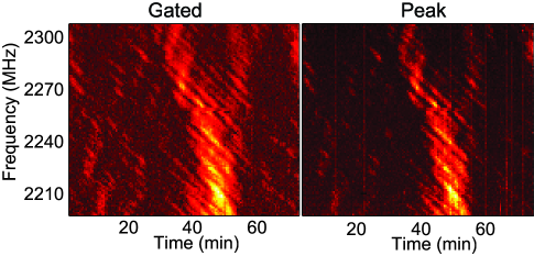
Figure 1: Comparison of dynamic spectra calculated using two different methods. The left and the right panels are for the gated-flux method and the peak-flux method respectively. Both methods produce similar results. The gated-flux method recovers low-flux structures better than that of peak-flux technique. The data was taken on April 1st 2014 with KM40m.

Being close to the near-by city Kunming, KM40m is highly affected by RFIs. There is no pulsar baseband recorder installed at KM40m at the time when the observations were carried out. In this way, we could not use voltage domain methods for RFI mitigation, e.g. the cyclic spectroscopy (Walker et al., 2013) and the spectral kurtosis method (Nita et al., 2007). For RFIs with persistent frequencies, we replace the RFI-affected channels using the linearly interpolation from the adjacent channels. We also interpolate in the time domain to remove spontaneous wideband RFIs. Occasionally, broadband RFIs last for a few minutes, and the resulted big data gap could not be repaired using the interpolation. We then treat the data of each part separately as different observations.

In total, we measured 25 independent dynamic spectra for PSR B0355+54. Fifteen of them have good signal-to-noise ratio, $S/N\geq 100$, and these data show structured patterns as in Figure 2. The other 10 observations have lower $S/N$, and we could not found clear structures after visual inspections. As one can see, these 15 high-$S/N$ dynamic spectra vary significantly as function of time. The dynamic spectra showed scintles with roughly 50-MHz bandwidth at beginning of January. The scintillation bandwidth reduced significantly in March, and over merely one day (MJD 56735 to 56736), the dynamic spectra developed into fringe-like structures. Such structures lasted for a month and turned into criss-cross structures in the early April, while the scintillation bandwidth was continuously reducing. Clearly, the scintillation parameters had changed significantly for PSR B0355+54. In next section, we provide quantitative analysis for such variations.

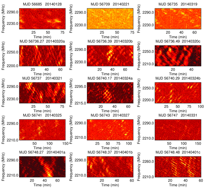
Figure 2: Dynamic spectra of PSR B0355+54 at centre frequency 2.25 GHz taken from January 28th 2014 to April 1st 2014. The epochs of observations are shown at the top of panels. The horizontal and vertical axes correspond to the time and the frequency, respectively.

3.2 The two-dimensional auto-correlation function

To obtain the scintillation bandwidth and the decorrelation time-scale, we compute the two-dimensional (2-D) ACF of the dynamic spectrum (Cordes, 1986; Gupta et al., 1994; Bhat et al., 1999a; Wang et al., 2008; Bhat et al., 2014), particularly, we follow the recipes from Cordes (1986) and Wang et al. (2008). The 2-D ACF, $F(\Delta\nu,\Delta\tau)$, is calculated from the pulsar flux, $S(\nu,t)$, as

$$F(\Delta\nu,\Delta\tau)=\sum_{\nu}\sum_{t}\Delta S(\nu,t)\Delta S(\nu+\Delta\nu,t+\Delta\tau)\,,$$ (1)

where $\nu$ is the channel frequency, $t$ is the time, $\Delta\nu$ and $\Delta\tau$ are correlation bandwidth and timescale respectively. The variation of flux is defined as $\Delta S(\nu,t)=S(\nu,t)-\overline{S(\nu,t)}$. We can normalise the 2-D ACF using its value at the zero lag and the normalised ACF ($\rho$) is

$$\rho(\triangle\emph{v},\Delta\tau)=F(\triangle\emph{v},\Delta\tau)/F(0,0)\,.$$ (2)

The contour plots of the normalised ACFs are shown in Figure 3, and the corresponding one-dimensional ACF along the time and frequency axes are shown in Figure 4 and Figure 5.

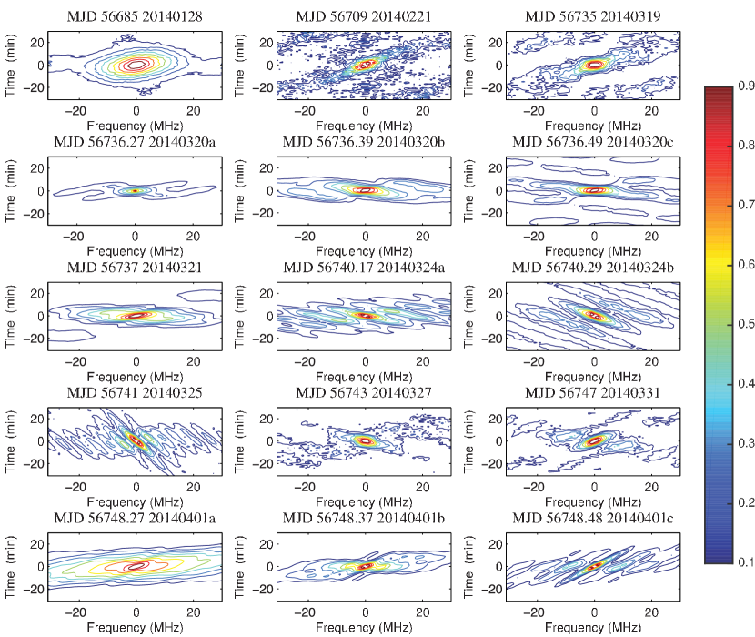
Figure 3: Contour plots of normalised ACF of dynamic spectra shown in Figure 2. The value of each contour is indicated using the colour bar on the right side.

Figure 4: One dimensional ACF in time, i.e. the $\Delta\tau_{\rm d}$-cross section of the two-dimensional ACF. The solid line is the measured value, and the dotted lines are from the best fitted two-dimensional elliptical Gaussian function as explained in the main text.

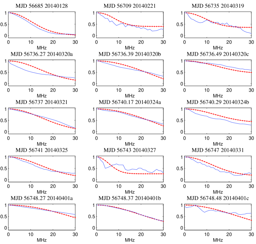
Figure 5: Similar to Figure 4, but the one dimensional ACF in frequency. The solid line is the measured value, and the dotted lines are from the best fitted two-dimensional elliptical Gaussian function.

We use 2-D Gaussian fitting (Wang et al., 2008) to determine the scintillation parameters $\Delta\tau_{\rm d}$ and $\Delta\nu_{\rm d}$ according to the model that

$$\rho_{\rm model}(\Delta\nu_{\rm d},\Delta\tau_{\rm d})=e^{-C_{1}\Delta\nu_{\rm d}^{2}-C_{2}\Delta\nu_{\rm d}\Delta\tau_{\rm d}-C_{3}\Delta\tau_{\rm d}^{2}}\,.$$ (3)

The parameters $C_{1}$, $C_{2}$, and $C_{3}$ describe the size and the orientation of elliptic of ACF. If we organised the coefficients $C_{1,2,3}$ in to matrix $\rm\bf C$

$${\rm\bf C}=\left(\begin{tabular}[]{c c}$C_{1}$&${C_{2}}/{2}$\\ ${C_{2}}/{2}$&$C_{3}$\end{tabular}\right)\,.$$ (4)

the orientation and size of the elliptic can be found using eigenvector and eigen values of matrix $\rm\bf C$ as shown in Lee et al. (2012).

Such the Gaussian fitting is empirical, e.g. the Kolmogorov turbulent spectrum predicts power-law correlation instead of Gaussian correlation (Rickett et al., 2014). However, in order to compare the results of previous works, we keep such Gaussian fitting convention. The discrimination of the correlation function types is left for the future investigation.

We infer the values of $C_{1},C_{2}$ and $C_{3}$ using the two dimensional $\chi^{2}$ fitting which minimises

$$\chi^{2}=\sum_{\Delta\nu_{\rm d},\Delta\tau_{\rm d}}\left[\rho(\Delta\nu_{\rm d},\Delta\tau_{\rm d})-\rho_{\rm model}(\Delta\nu_{\rm d},\Delta\tau_{\rm d})\right]^{2}\,.$$ (5)

Following the usual conventions (Bhat et al., 1999a; Wang et al., 2008), the scintillation time scale $\Delta\tau_{\rm d}$ is the half width of time lag producing $\rho=1/e$, and the decorrelation bandwidth scale $\Delta\nu_{\rm d}$ is the half-width of frequency lag giving $\rho=1/2$. The scintillation parameters $\Delta\nu_{d}$ and $\Delta\tau_{d}$ are calculated as

$$\Delta\nu_{d} = \sqrt{\ln 2/C_{1}}\,,$$ (6)

$$\Delta\tau_{d} = 1/\sqrt{C_{3}}\,.$$ (7)

The error of estimated parameters come from two major sources, i) the statistical error as computed from the $\chi^{2}$ fitting procedure (Press et al., 2007), and ii) the error due to a finite number of bright scintles in the given data (Cordes, 1986). The fractional error of the second type is (Cordes, 1986; Bhat et al., 2014) $\sigma\simeq f^{-1/2}(\Delta\tau_{\rm d}/T)^{1/2}(\Delta\nu_{\rm d}/{\rm BW})^{1/2}$, where $T$ and ${\rm BW}$ are the data duration, and bandwidth. The filling factor, $f$, is the ratio between the area of bright scintles and the area for a single feature in the dynamic spectrum, which is choose as $f=0.2$ in the current paper.

We summarise the measured values of $\Delta\nu_{\rm d}$ and $\Delta\tau_{\rm d}$ in Table. 1 and Figure 6. Our measurements agree with the predication of the Galactic free electron density model NE2001 (Cordes & Lazio, 2002), where the predicted scintillation decorrelation bandwidth and timescale of PSR B0355+54 are 25 MHz and 390 s at the central frequency of 2.25 GHz, assuming a transverse velocity of 100 km/s.

Table 1: Scintillation parameters for each epoch. The sup-script $a,b$ and $c$ indicate that we have split the session due to the RFI reason. $\Delta\tau_{\rm d}$ and $\Delta\nu_{\rm d}$ are the scattering timescale and decorrelation bandwidth respectively. The $\alpha$ and $w$ are the curvature and width of the scintillation arcs. $d$ is the scattering screen-Earth distance infered from the arc curvature, where we had neglected the annual variations of Earth velocity due to the limited time span and used reference value of $V_{\rm eff,\perp}=100$ km/s. The detailed definitions are delayed in Section  3.3. For numbers with two values of error, the first error is the statistical error, while the second is the finite-sample error as we had explained. We quote the logarithmic value of arc curvature, because the confidence level contours are more symmetric in logarithmic scale than linear as shown in Figure 9.

Epoch	Duration	Bandwidth	$\Delta\tau_{d}$	$\Delta\nu_{\rm d}$	$\alpha$	$w$	$d_{\rm eff}$	$S/N$
MJD	min	MHz	min	MHz	$\log(\mu$s$\cdot$min${}^{2})$	$10^{-2}\mu$s	kpc
56685	80	110	6.1$\pm$0.2$\pm$1.2	11.8$\pm$0.2$\pm$2.4	$0.6^{+0.8}_{-1.0}$	$9^{+16}_{-7}$	0.2	140
56709	76	100	2.5$\pm$0.2$\pm$0.2	3.9$\pm$0.3 $\pm$0.3	$0.5^{+0.1}_{-0.3}$	$9^{+6}_{-5}$	0.2	137
56735	70	100	3.0$\pm$0.2$\pm$0.3	6.0$\pm$0.3 $\pm$0.7	$0.3^{+0.2}_{-0.1}$	$8^{+2}_{-4}$	0.1	136
56736a	84	61	2.9$\pm$0.2$\pm$0.6	16.5$\pm$0.2$\pm$3.6	$-0.1^{+0.05}_{-0.3}$	$7^{+18}_{-3}$	0.03	331
56736b	73	100	4.5$\pm$0.1 $\pm$1.3	29$\pm$1.0$\pm$8.7	$-0.1^{+0.2}_{-0.1}$	$8^{+6}_{-3}$	0.03	338
56736c	51	67	2.0$\pm$0.2 $\pm$0.3	10.3$\pm$0.3$\pm$1.8	$-0.1^{+0.1}_{-0.1}$	$9^{+6}_{-3}$	0.03	434
56737	80	100	3.4$\pm$0.1 $\pm$0.6	16.9$\pm$0.5$\pm$3.2	$-0.2^{+0.1}_{-0.1}$	$11^{+3}_{-5}$	0.03	576
56740a	67	100	7.3$\pm$0.3 $\pm$3.0	32$\pm$1.0$\pm$13	$-0.2^{+0.3}_{-0.1}$	$21^{+7}_{-9}$	0.03	296
56740b	100	71	5.2$\pm$0.5 $\pm$1.2	16$\pm$1.0$\pm$3.8	$0.6^{+0.1}_{-0.3}$	$13^{+8}_{-5}$	0.2	316
56741	150	100	6.9$\pm$0.5$\pm$1.3	16.6$\pm$0.9$\pm$3.2	$0.5^{+0.1}_{-0.2}$	$16^{+5}_{-6}$	0.2	281
56743	110	115	5.0$\pm$0.4$\pm$0.8	12.3$\pm$0.8$\pm$1.9	$0.3^{+0.7}_{-0.7}$	$12^{+6}_{-9}$	0.1	161
56747	160	110	3.9$\pm$0.3$\pm$0.4	11.1$\pm$0.7$\pm$1.2	$0.1^{+0.3}_{-0.2}$	$13^{+7}_{-7}$	0.06	156
56748a	80	110	7.2$\pm$0.1$\pm$2.7	34.6$\pm$0.7$\pm$13	$0.0^{+0.1}_{-0.1}$	$14^{+8}_{-6}$	0.05	558
56748b	77	110	3.7$\pm$0.1$\pm$0.7	16.7$\pm$0.6$\pm$3.2	$-0.1^{+0.3}_{-0.4}$	$17^{+6}_{-10}$	0.03	368
56748c	75	81	5.0$\pm$0.3$\pm$1.4	20$\pm$1.0$\pm$5.7	$-0.1^{+0.2}_{-0.2}$	$18^{+9}_{-6}$	0.03	235

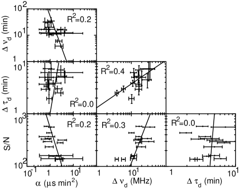
Figure 6: The correlation between $S/N$, scintillation time scale, scintillation bandwidth, and arc curvature with values from Table. 1. The solid line are the power-law function fitting. The value of $R^{2}$ in each panel is the coefficient of determination. Except $S/N-\Delta\tau_{\rm d}$ and $S/N-\Delta\tau_{\rm d}$ parameter pairs, the other parameter pairs show marginal correlation. Using the $\Delta\tau_{\rm d}-\Delta\nu_{\rm d}$ correlation, we can measure the transverse velocity of PSR B0355$+$54, that $V/\sqrt{\eta}=310\pm 100$ km/s, assuming pulsar distance $D=1.0$ kpc (Chatterjee et al., 2003).

For the thin-screen model of diffractive scintillation, the scattering time scale and the bandwidth follow a simple relation that (Gupta et al., 1994; Wang et al., 2008)

$$\Delta\tau_{\rm d}=6.4\times 10^{2}\eta^{\frac{1}{2}}\left(\frac{D}{\rm kpc}\right)^{\frac{1}{2}}\left(\frac{\Delta\nu_{\rm d}}{\rm MHz}\right)^{\frac{1}{2}}\left(\frac{V}{\rm km/s}\right)^{-1}\left(\frac{\nu}{\rm GHz}\right)^{-1}{\rm min}\,,$$ (8)

where the $D$ and $V$ are the pulsar scintillation distance and velocity respectively, $\eta$ is the ratio between the screen-to-observer distance and screen-to-pulsar distance. One can find the measured $\Delta\tau_{\rm d}-\Delta\nu_{\rm d}$ relation in Figure 6. After fixing the pulsar distance to the interferometry distance $1.0$ kpc (Chatterjee et al., 2003), we can fit the data using Equation. 8 to get the pulsar scattering velocity $V/\sqrt{\eta}=340\pm 130$ km/s. Comparing to the interferometry velocity of 61 km/s (Chatterjee et al., 2003), one would require $\eta\simeq 0.01-0.1$, i.e. a rather nearby scattering screen locates $0.01-0.1$ kpc away from the Earth in the pulsar direction.

3.3 Secondary Spectrum

The secondary spectrum $\cal S$ is the two-dimensional Fourier transform of a dynamic spectrum. Parabolic shaped structures (i.e. the scintillation arcs) are expected in the secondary spectrum (Walker et al., 2004; Cordes et al., 2006) under two conditions, 1) the scattering is anisotropic that the interference is dominated by only a few scattering directions; and 2) there is enough time-frequency resolution and high $S/N$.

At lower frequencies, Stinebring (2006) had already detected scintillation arcs for the PSR B0355+54, indicating the anisotropic scatterings. The flux of PSR B0355+54 is 23 mJy at L-band, and its scattering timescale and bandwidth are at the level of a few minutes and tens of MHz. All these make PSR B0355+54 a potential target to search for the scintillation arcs at the 2.25 GHz.

The secondary spectra of our observations are plotted in Figure 7. In multiple epochs, the scintillation arcs are clearly visible. For epochs of March 20th 2014, March 24th 2014, and probably 1st April 2014, there may be hints for the inverted arclets, but the limited $S/N$ and spectral resolution prevent us from studying the details.

Walker et al. (2004) and Cordes et al. (2006) had explained the physics behind scintillation arcs. We have prepared a pictorial illustration in Appendix A to explain the relation between the scintillation arc and the intensity distribution of scattered radiation. Basically, the scintillation arcs come from the coherent interference between a limited number of signal propagating paths.

For the most simple case, where the radiation gets scattered into only two directions, ${\boldsymbol{\theta}}_{1}$ and ${\boldsymbol{\theta}}_{2}$, the intensities of the secondary spectrum will distribute around those conjugate frequency ($f_{\nu}$) and conjugate time ($f_{\rm t}$) with

$$f_{v} = \frac{D\eta}{2c}\left(\theta_{2}^{2}-\theta_{1}^{2}\right)\,,$$ (9)

$$f_{t} = \frac{1+\eta}{\lambda}({\boldsymbol{\theta}}_{2}-{\boldsymbol{\theta}}_{1})\cdot{\rm\bf V}_{\rm eff}\,.$$ (10)

Here, $\lambda$ is the observing wavelength, the effective perpendicular velocity (${\rm\bf V}_{\rm eff,\perp}$) is defined as

$${\rm\bf V}_{\rm eff,\perp}={\rm\bf V}_{\rm psr,\perp}\frac{\eta}{1+\eta}+{\rm\bf V}_{\rm obs,\perp}\frac{1}{1+\eta}-{\rm\bf V}_{\rm screen,\perp}\,,$$ (11)

and ${\rm\bf V}_{\rm psr},\perp$, ${\rm\bf V}_{\rm obs,\perp}$, and ${\rm\bf V}_{\rm screen,\perp}$ are the transverse velocity of pulsar, observer, and screen respectively (Cordes & Rickett, 1998).

From Equation. 9 and 10, one can see that the $f_{\rm\nu}=\alpha f_{\rm t}^{2}$, if the major scattered intensities are at the origin ($\boldsymbol{\theta}_{1}=0$) and along a straight line passing through the origin, i.e. $\boldsymbol{\theta}_{2}=\theta{\rm\bf n}$ with $\rm\bf n$ being a unit vector in the scattering screen. In such a scenario, the intensity distribution in the secondary spectrum will be the parabolic arc with a curvature of

$$\alpha=\frac{D\eta\lambda^{2}}{2c({\rm\bf V}_{\rm eff,\perp}\cdot{\rm\bf n})^{2}(1+\eta)^{2}}\,.$$ (12)

As shown in Figure 7, our observed scintillation arcs vary over the 90 days, particularly, the curvature of arcs and distribution of intensity along the arc change temporally. Due to the limited $S/N$, we can not study the arc variation by tracing the arclets as in Stinebring (2006) or Trang & Rickett (2007). Alternatively, we designed a statistics $S^{\prime}$ to do so. The statistics is similar to the generalised Hough transformation (Ballard, 1981). We re-parameterise the parameter space of $f_{\rm\nu}$ and $f_{\rm t}$ using the other two parameters, the parabolic width $w$ and arc curvature $\alpha$. The transformation is defined as the difference between the reduced $\chi^{2}$ of secondary spectrum in the two complementary regions $\Theta_{1}$ and $\Theta_{2}$. As illustrated in Figure 8, the region $\Theta_{1}$ contains the given arc and the region $\Theta_{2}$ does not.

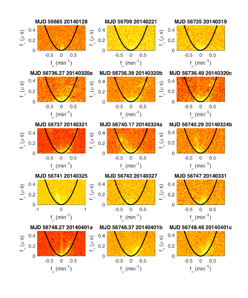
Figure 7: Secondary spectra for the PSR B0355+54 displayed using a logarithmic colour scale, i.e. $\log{\cal S}$. The x-axis and y-axis are the conjugate time ($f_{\rm t}$) and conjugate frequency ($f_{\rm\nu}$). The parabolic shaped scintillation arcs can be spotted for most of the epochs. The black solid parabolic curve indicates the weighted average curvature $\bar{\alpha}$, see Equation 17 and related discussions for the details.

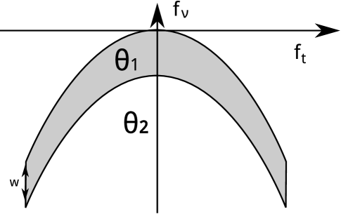
Figure 8: The parameter space $\Theta_{1}$ and $\Theta_{2}$ for Equation. 13. The $\Theta_{1}$ is the parameter space spanned by the arc with curvature of $\alpha$ passing the origin and the arc parallely shifted by $w$ along $f_{\rm\nu}$ axis, i.e. the parameter space in the parabolic belt with width of $w$. The statistics $S^{\prime}$ is defined as the difference between the reduced $\chi^{2}$ of $\log\cal S$ in the region $\Theta_{1}$ and $\Theta_{2}$.

The statistics $S^{\prime}$ is defined as

$${S^{\prime}}=\sum_{\{f_{\rm\nu}f_{\rm t}\}\in\Theta_{\rm 1}}\frac{\log{\cal S}}{N_{\Theta_{1}}\sigma_{\log\cal S}}-\sum_{\{f_{\rm\nu}f_{\rm t}\}\in\Theta_{\rm 2}}\frac{\log{\cal S}}{N_{\Theta_{2}}\sigma_{\log\cal S}}\,,$$ (13)

where the region $\Theta_{1}$ in the $f_{\rm t}-f_{\rm\nu}$ space covers the parabolic arc with the curvature of $\alpha$ and its width $w$ along the positive $f_{\rm\nu}$ direction, as illustrated in Figure 8. The complementary region $\Theta_{2}$ covers the rest of $f_{\rm t}-f_{\rm\nu}$ space. We denote the standard deviation of $\log S$ as $\sigma_{\log\cal S}$. The number of data points in the two regions $\Theta_{1}$ and $\Theta_{2}$ are denoted as $N_{\Theta_{1}}$ and $N_{\Theta_{2}}$ respectively.

The statistics $S^{\prime}$ is defined using logarithm of secondary spectrum, because the probability distribution of $S$ is very close to the log-normal distribution. The statistics $S^{\prime}$, therefore, describes the significance of the difference between the mean of $\log S$ in the regions $\Theta_{1}$ and $\Theta_{2}$. The distribution of $S^{\prime}$ under the null hypothesis that there is no arc-like structure in the secondary spectrum follows the Student’s $t$-distribution, and we can use the $t$-test to compute the confidence level of $w$ and $\alpha$.

With $S^{\prime}$, we can measure the arc curvature and the direction of scattering, where the arc width $w$ is used to infer scattering angle $\theta_{\rm y}$ as illustrated in Figure 11 of Appendix. A that

$$\theta_{\rm y}=\sqrt{\frac{2cw}{D\eta}}\,.$$ (14)

We note that a recent work (Bhat et al., 2016) is similar in analysing the secondary spectra. There are differences between Bhat et al. 2016 and the current work. Firstly, the statistics are chosen differently. Bhat et al. (2016) integrated scintillation power along the path of parabolic arc with a fixed pixel width, then measured the arc curvature. We rely on the statistics $\cal S^{\prime}$ to perform the parameter inference. The statistics $\cal S^{\prime}$ is the likelihood ratio test and it is also the matched filter to detect power difference (DiFranco & Rubin, 1968). Secondly, we perform statistical inference simultaneously on the two parameters, $w$ and $\alpha$, while in Bhat et al. (2016) $w$ is fixed. As the two parameters show clear correlation, we prefer to use the current two-parameter approach to get reliable error estimation (see more discussion in Press et al. (2007)).

The measured $S^{\prime}$ as a function of $\alpha$ and $w$ are shown in Figure 9. As one can see that the most of the spectral energy concentrates around a particular value of $\alpha$ and $w$. The value of width $w$ is about $0.1{\rm\mu s}$. According to Equation 14, the corresponding the angular scale of scattered radiation is 0.2 mas. We can also derive the effective scattering screen distance from the arc curvature $\alpha$ via $d_{\rm eff}=2\alpha c{V}_{\rm eff,\perp}^{2}(1+\eta)/\lambda^{2}$ (see Eq. 12). The effective scattering scattering distance is defined as

$$d_{\rm eff}\equiv\frac{D\eta}{(1+\eta)\cos^{2}\theta_{\rm\perp}}\,,$$ (15)

where the angle $\theta_{\rm\perp}$ is the angle between the scattering position $\rm\bf n$ and the transverse effective velocity ${\rm\bf V}_{\rm eff,\perp}$. We list the measured $d_{\rm eff}$ in Table. 1, which agree with the distance estimation from the $\Delta\tau_{\rm d}-\Delta\nu_{\rm d}$ relations.

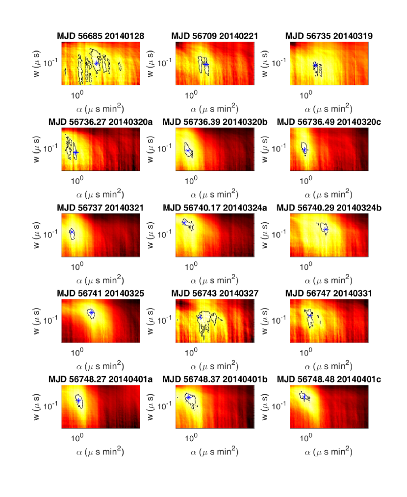
Figure 9: The transformed secondary spectra $\cal S^{\prime}$ as function of curvature $\alpha$ and width $w$ according to Eq. 13. The black contours are for ‘1-$\sigma$’ confidence level, and ‘*’ symbol indicates the most probable values for $\alpha$ and $w$.

We use the $\chi^{2}$ test to check if the arc curvature is varying. Here the null hypothesis $H_{0}$ and positive hypothesis $H_{1}$ are

$$\left\{\begin{array}[]{l}\text{$H_{0}$: arc curvature is a constant,}\\ \text{$H_{1}$: arc curvature is varying.}\end{array}\right.$$

Under the $H_{0}$, the statistics $\chi^{2}$ is defined as

$$\chi^{2}=\sum_{i}\left(\frac{\alpha_{i}-\bar{\alpha}}{\sigma_{\alpha,i}}\right)^{2}\,$$ (16)

which follows the $\chi^{2}$ distribution with degree of freedom of $N-1$. Here, $i$ is the index of observation session and $N$ is the total number of data points. The weighted average value $\bar{\alpha}$ is defined as

$$\bar{\alpha}=\frac{\sum_{i}\alpha_{i}\sigma_{\alpha,i}^{-2}}{\sum_{i}\sigma_{\alpha,i}^{-2}}\,,$$ (17)

where $\sigma_{\alpha,i}$ is the error of $\alpha_{i}$

Since the errorbars of data points are asymmetric, the error $\sigma_{\rm\alpha_{i}}$ is chosen accordingly depending on whether curvature $\alpha_{i}$ is larger or smaller than $\bar{\alpha}$. Using the values in Table. 1, we get $\chi^{2}=40$. The corresponding P-value is $\leq 2\times 10^{-4}$ under $H_{0}$, i.e. we can rule out the hypothesis that the arc curvature is a constant with the probability of making mistake no more than $2\times 10^{-4}$ (more confident than the ‘3.5-$\sigma$’). From the transformed secondary spectra, one can visually see how the arc curvature varies epoch-to-epoch. In Figure 7, we also draw curves to indicate the weighted mean $\bar{\alpha}$ for comparisons.

As a summary, we collect all the temporal variation of scattering bandwidth, scattering timescale, arc curvature, width, and $S/N$ in Figure 10 and Table 1. Due to the lack of noise calibrator at the site, we can not convert the $S/N$ to the radio flux. In this way, $S/N$ is only for the reference purpose. The $S/N$ is defined as the ratio between the integrated intensity and noise intensity as computed by PSRCHIVE (Hotan et al., 2004).

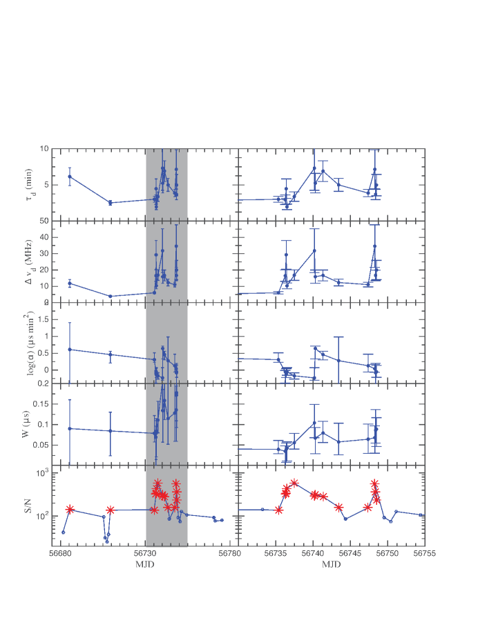
Figure 10: The temporal variation of scattering timescale $\Delta\tau_{\rm d}$, bandwidth $\Delta\nu_{\rm d}$, arc curvature $\alpha$, arc width $w$, and $S/N$. The x-axis is the epoch of observation. One can see that all those parameters are temporally variable except the arc width $w$. The right panels show the zoomed regions indicated by the grey shading in the left panels. In the $S/N$ panel, the $*$ symbols indicate the observation epochs showing scintillation arcs. The open circles are the epochs showing no arcs.

From Figure 10, one can see that four scattering parameters vary temporally, i.e. the scattering bandwidth, the scattering timescale, the arc curvature, and $S/N$. We have also checked the correlation between $\Delta\tau_{\rm d}$, $\Delta\nu_{\rm d}$, $S/N$, and arc curvature as in Figure 6. We have used the coefficient of determination $R^{2}$, the fractional reduction of total sum of squares , to describe the correlation between the four parameters. There is indication for correlation between $\Delta\nu_{\rm d}$-$S/N$, and $\alpha$-$S/N$. There also seems to be an anti-correlation between the arc curvature ($\alpha$) and scattering bandwidth ($\Delta\nu_{\rm d}$).

4 Discussions and Conclusions

In this paper, we had studied the scintillation of radio radiation from PSR B0355+54 using the Kunming 40m radio telescope at 2.25 GHz. We had measured the dynamic spectra of PSR B0355+54 for 15 epochs. Using the ACF method, we have inferred the scattering timescale and bandwidth, which agree with the predication of the NE2001 model. We used the generalised Hough transform to measure and to study the curvature and scattering directions.

Although the arclets are not resolved in our measured secondary spectra, we can see the arc are asymmetric with respects to the $f_{\rm t}$ axis. We can see such $f_{\rm t}$-axis mirror symmetry of scintillation arc varies on time scale of days, which indicates that the asymmetry of interstellar scattering medium at the 0.1-AU scale, assuming velocity scale of $100$ km/s. This agrees with results of Brisken et al. (2010).

If we interpret our result in the thin screen scintillation model, then our inferred scintillation screen will be very nearby (0.01-0.1 kpc). By comparing to the geometry of local ISM structure of Bhat & Gupta (2002), our scattering screen seems to be at the edge of the Local Bubble. However, due to the complexity in the Local bubble and Perseus cloud (Lallement et al., 2014; Yao et al., 2017), it is still premature to drew conclusions.

A feature can be noted in both Figure 7, 9, and 10, that the arc curvature varies on a rather short timescale of days. For example, from March 24th 2014 (MJD 56740) to March 25th 2014 (MJD 56741), the arc curvature increased from $\log\alpha=-0.2\log{\rm\mu s\cdot min^{2}}$ to $0.6\log{\rm\mu s\cdot min^{2}}$ and later decrease to $-0.1\log{\rm\mu s\cdot min^{2}}$ at April 1st 2014 (MJD 56748). This is surprising, because the curvature is thought to be determined by pulsar distance, effective velocity, and screen position. Pulsar distance clearly can be regarded as a constant over 90 days. The earth velocity and screen velocity should be comparable to the proper motion of PSR B0355+54. Earth velocity mainly leads to an annual variation of arc curvature (Stinebring, 2006), and will not contribute to the day-timescale variation we found here. The reason of such short timescale variation of curvature, thus, should be either 1) the variation of distance ratio $\eta$ of scattered screen or 2) the angle between transverse velocity and scattering direction, i.e. $\theta_{\rm\perp}$ in Eq. 15 or 3) only the inner edge the scintillation arc is visible for epochs with higher $\alpha$. In the first scenario, scattering screens with different distance dominate the scattering at different epochs (Stinebring, 2006, 2007). In the second scenario, pattern of the scattering structure changes or different scintillas dominate the interference (Brisken et al., 2010). In the third scenario, one requires the arclets be highly asymmetric. Our detection of anti-correlation between arc curvature ($\alpha$) and scintillation bandwidth $\Delta\nu_{\rm d}$ seems to prefer the first interpretation. A dedicated pulsar monitoring using interferometer (Brisken et al., 2010; Bassa et al., 2016) may help to resolve the three possibilities.

The resolution of our secondary spectrum is limited, in fact, by RFIs. The observation bandwidth is limited by the RFIs, so the $f_{\rm\tau}$ resolution is limited. Splitting data into different segmentation reduces data length, so do the resolution for $f_{\rm\nu}$.

It seems whether we can observe the scintillation arc is related to the value of $S/N$. As shown in Figure 10, we did not find scintillation arcs in epoch with $S/N$ slightly below the threshold of $100$. In principle, whether one observes the scintillation arc depends not only on the $S/N$, but also the anisotropy of scattering. We expected that future telescopes with higher sensitivity, e.g. FAST(Nan et al., 2011), QTT(Wang, 2017), or SKA(Han et al., 2015) will be beneficial in the pulsar scintillation studies.

Appendix A Pictorial introduction to the scintillation arc

In Figure 11, we use cartoon figures to illustrate the relation between the scintillation arc and the scattered intensity for a few highly simplified scenarios. The details for the modeling can be found in Walker et al. (2004) and Cordes et al. (2006).

Three cases are shown here. In all cases, the interference happens between a localised central radiation and a strip-shaped scattered radiation (see Pen & Levin (2014) for a possible physical explanation of such 1-D structure and Coles et al. (2010) for a more detailed simulation). In the first case, the effective velocity lies along the elongate direction of strip-shaped radiations; and the strip structure overlays with centre radiation. In the second case, the strip structure gets shifted perpendicular to the direction of effective velocity. The third case is similar to the second, except that the effective velocity and elongating direction of radiation strip are misaligned. The figure here show how such shifts and misalignments of radiation strip structure lead to the corresponding shifts of parabolic scintillation arc in the $f_{\nu}$-$f_{\rm t}$ parameter space.

Clearly, if the strip components have certain width along the $\theta_{\rm y}$ direction, the scintillation arc will gain finite width ($w$ defined in Figure. 8), which is determined by the angular scale $\Delta\theta_{\rm y}$ as shown in the figure.

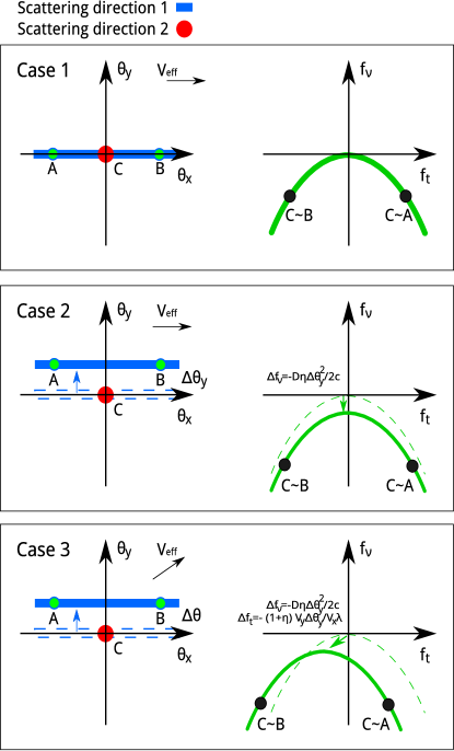
Figure 11: Cartoon illustrations for the relations between scattered intensity distribution and scintillation arcs. The left panels are the distribution of scattered intensity. The right panels are the corresponding scintillation arcs in the secondary spectra. Here the $V_{\rm eff}$ is the effective velocity, and the arrow indicates it direction. For the most simple case, the scattered intensity is dominated by two major components, a central component $C$, and a strip structure $A-B$. The interference between point $A$ and $C$ is mapped into the $C\sim A$, and similarly, the $B$-$A$ interference is mapped into $B\sim A$. For the ‘Case 2’ and ‘3’, the value of arc shift in $f_{\rm t}$ and $f_{\rm\nu}$ parameter space are given in the figure.

References

- Armstrong et al. (1995) Armstrong J. W., Rickett B. J., Spangler S. R., 1995, ApJ, 443, 209
- Ballard (1981) Ballard D., 1981, Pattern Recognition, 13, 111
- Bassa et al. (2016) Bassa C. G., Janssen G. H., Karuppusamy R., Kramer M., Lee K. J., Liu K., McKee J., Perrodin D., Purver M., Sanidas S., Smits R., Stappers B. W., 2016, MNRAS, 456, 2196
- Bhat et al. (2014) Bhat N. D. R., et al., 2014, ApJL, 791, L32
- Bhat & Gupta (2002) Bhat N. D. R., Gupta Y., 2002, ApJ, 567, 342
- Bhat et al. (2016) Bhat N. D. R., Ord S. M., Tremblay S. E., McSweeney S. J., Tingay S. J., 2016, ApJ, 818, 86
- Bhat et al. (1999a) Bhat N. D. R., Rao A. P., Gupta Y., 1999a, ApJs, 121, 483
- Bhat et al. (1999b) Bhat N. D. R., Rao A. P., Gupta Y., 1999b, ApJ, 514, 272
- Brisken et al. (2010) Brisken W. F., Macquart J.-P., Gao J. J., Rickett B. J., Coles W. A., Deller A. T., Tingay S. J., West C. J., 2010, ApJ, 708, 232
- Chatterjee et al. (2003) Chatterjee S., Cordes J. M., Lazio T. J. W., 2003, in Bailes M., Nice D. J., Thorsett S. E., eds, Radio Pulsars Vol. 302 of Astronomical Society of the Pacific Conference Series, Probing the Galaxy with Pulsar Parallaxes and Proper Motions. p. 225
- Coles et al. (2010) Coles W. A., Rickett B. J., Gao J. J., Hobbs G., Verbiest J. P. W., 2010, ApJ, 717, 1206
- Cordes (1986) Cordes J. M., 1986, ApJ, 311, 183
- Cordes & Lazio (2002) Cordes J. M., Lazio T. J. W., 2002, ArXiv Astrophysics e-prints
- Cordes & Rickett (1998) Cordes J. M., Rickett B. J., 1998, ApJ, 507, 846
- Cordes et al. (2006) Cordes J. M., Rickett B. J., Stinebring D. R., Coles W. A., 2006, ApJ, 637, 346
- Cordes & Wolszczan (1986) Cordes J. M., Wolszczan A., 1986, ApJL, 307, L27
- DiFranco & Rubin (1968) DiFranco J. V., Rubin W. L., 1968, Radar Detection. Prentice-Hall Electrical Engineering Series, Prentice-Hall INC
- Gupta et al. (1994) Gupta Y., Rickett B. J., Lyne A. G., 1994, MNRAS, 269, 1035
- Han et al. (2015) Han J. L., van Straten W., Lazio T. J. W., Deller A., Sobey C., Xu J., Schnitzeler D., Imai H., Chatterjee S., Macquart J.-P., Kramer M., Cordes J. M., 2015, Advancing Astrophysics with the Square Kilometre Array (AASKA14), p. 41
- Hewish et al. (1985) Hewish A., Wolszczan A., Graham D. A., 1985, MNRAS, 213, 167
- Hotan et al. (2004) Hotan A. W., van Straten W., Manchester R. N., 2004, PASA, 21, 302
- Lallement et al. (2014) Lallement R., Vergely J.-L., Valette B., Puspitarini L., Eyer L., Casagrande L., 2014, A&A, 561, A91
- Lee et al. (2012) Lee K. J., Guillemot L., Yue Y. L., Kramer M., Champion D. J., 2012, MNRAS, 424, 2832
- Nan et al. (2011) Nan R., Li D., Jin C., Wang Q., Zhu L., Zhu W., Zhang H., Yue Y., Qian L., 2011, International Journal of Modern Physics D, 20, 989
- Narayan (1992) Narayan R., 1992, Philosophical Transactions of the Royal Society of London Series A, 341, 151
- Nita et al. (2007) Nita G. M., Gary D. E., Liu Z., Hurford G. J., White S. M., 2007, PASP, 119, 805
- Pen & Levin (2014) Pen U.-L., Levin Y., 2014, MNRAS, 442, 3338
- Press et al. (2007) Press W. H., Teukolsky S. A., Vetterling W. T., Flannery B. P., 2007, Numerical Recipes 3rd Edition: The Art of Scientific Computing, 3 edn. Cambridge University Press, New York, NY, USA
- Rickett et al. (2014) Rickett B. J., Coles W. A., Nava C. F., McLaughlin M. A., Ransom S. M., Camilo F., Ferdman R. D., Freire P. C. C., Kramer M., Lyne A. G., Stairs I. H., 2014, ApJ, 787, 161
- Stinebring (2007) Stinebring D., 2007, in Haverkorn M., Goss W. M., eds, SINS - Small Ionized and Neutral Structures in the Diffuse Interstellar Medium Vol. 365 of Astronomical Society of the Pacific Conference Series, Pulsar Scintillation Arcs and the Ionized ISM. p. 254
- Stinebring (2006) Stinebring D. R., 2006, Chinese Journal of Astronomy and Astrophysics Supplement, 6, 204
- Stinebring et al. (2001) Stinebring D. R., McLaughlin M. A., Cordes J. M., Becker K. M., Goodman J. E. E., Kramer M. A., Sheckard J. L., Smith C. T., 2001, ApJL, 549, L97
- Trang & Rickett (2007) Trang F. S., Rickett B. J., 2007, ApJ, 661, 1064
- Walker et al. (2013) Walker M. A., Demorest P. B., van Straten W., 2013, ApJ, 779, 99
- Walker et al. (2004) Walker M. A., Melrose D. B., Stinebring D. R., Zhang C. M., 2004, MNRAS, 354, 43
- Wang (2017) Wang N., 2017, Scientia Sinica Physica, Mechanica & Astronomica, 47, 059501
- Wang et al. (2008) Wang N., Yan Z., Manchester R. N., Wang H. X., 2008, MNRAS, 385, 1393
- Yao et al. (2017) Yao J. M., Manchester R. N., Wang N., 2017, ApJ, 835, 29