prDeep: Robust Phase Retrieval with a Flexible Deep Network

Abstract

Phase retrieval algorithms have become an important component in many modern computational imaging systems. For instance, in the context of ptychography and speckle correlation imaging, they enable imaging past the diffraction limit and through scattering media, respectively. Unfortunately, traditional phase retrieval algorithms struggle in the presence of noise. Progress has been made recently on more robust algorithms using signal priors, but at the expense of limiting the range of supported measurement models (e.g., to Gaussian or coded diffraction patterns). In this work we leverage the regularization-by-denoising framework and a convolutional neural network denoiser to create prDeep, a new phase retrieval algorithm that is both robust and broadly applicable. We test and validate prDeep in simulation to demonstrate that it is robust to noise and can handle a variety of system models.

1 Introduction

The PR problem manifests when one wants to recover the input from only the amplitude, or intensity, of the output of a linear system. Mathematically, PR refers to the problem of recovering a vectorized signal $x\in\mathbb{R}^{n}~{}\text{or}~{}\mathbb{C}^{n}$ from measurements $y$ of the form

$$y=|\mathbf{A}x|+w,$$ (1)

where the measurement matrix $\mathbf{A}$ represents the forward operator of the system and $w$ represents noise.

PR shows up in many imaging applications including microscopy (Zheng & Yang, 2013), crystallography (Millane, 1990), astronomical imaging (Dainty & Fienup, 1987), and inverse scattering (Katz et al., 2014; Metzler et al., 2017b), to name just a few.

PR algorithms were first developed in the early 1970s and have been continuously studied by the optics community since then (Gerchberg, 1972; Fienup, 1978, 1982; Griffin & Lim, 1984; Pfeifer et al., 2006; Rodriguez et al., 2013). More recently, PR has been taken up by the optimization community. This has produced a number of algorithms with theoretical, if not always practical, benefits (Candes et al., 2013, 2015a; Goldstein & Studer, 2016; Bahmani & Romberg, 2017). For a benchmark study of over a dozen popular PR algorithms, see PhasePack (Chandra et al., 2017).

Following the popularity of compressive sensing, numerous algorithms were developed that use prior information, oftentimes sparsity, to improve PR reconstructions and potentially enable compressive PR (Moravec et al., 2007; Schniter & Rangan, 2015). In general, these methods do not improve reconstructions when the signal of interest is dense.

In the last few years, three methods, SPAR (Katkovnik & Astola, 2012; Katkovnik, 2017), BM3D-prGAMP (Metzler et al., 2016b), and Plug-and-Play ADMM (Venkatakrishnan et al., 2013; Heide et al., 2016), have been developed to solve the PR problem using natural-image priors, which make their reconstructions more robust to noise. These methods all apply a natural-image prior via the BM3D image-denoising algorithm (Dabov et al., 2007).

Unfortunately, two of these three methods, SPAR and BM3D-prGAMP, are restricted to i.i.d Gaussian or coded diffraction measurements (Candes et al., 2015b), which prevents their use in many practical applications. All three methods are computationally demanding.

In this work, we make two technical contributions. First, we show how the Regularization by Denoising (RED) (Romano et al., 2017) framework can be adapted to solve the PR problem. We call this adaption prRED. Because it sets up a general optimization problem, rather than using a specific algorithm, prRED is flexible and can handle a wide variety of measurements including, critically, Fourier measurements.

Second, we show how prRED can utilize convolutional neural networks by incorporating the DnCNN neural network (Zhang et al., 2017). We call this combination of RED and DnCNN applied to PR prDeep.

prDeep offers excellent performance with reasonable run times. In Section 4, we apply prDeep to simulated data and show that it compares favorably to existing algorithms with respect to computation time and robustness to noise.

2 Related Work

Our work fits into the recent trend of using advanced signal priors to solve inverse problems in imaging. While priors like sparsity, smoothness, and structured sparsity have been studied for some time, we focus here on plug-and-play priors and deep-learning priors, which together represent the state-of-the-art for a range of imaging recovery tasks.

2.1 Plug-and-Play Regularization for Linear Inverse Problems

Image denoising is arguably the most fundamental problem in image processing and, as such, it has been studied extensively. Today there exist hundreds of denoising algorithms that model and exploit the complex structure of natural images in order to remove additive noise.

Earlier this decade, researchers realized they could leverage these highly developed denoising algorithms to act as regularizers in order to solve other linear inverse-problems, such as deblurring, superresolution, and compressed sensing (Danielyan et al., 2010). This technique was eventually coined plug-and-play regularization (Venkatakrishnan et al., 2013), with the idea being that one could “plug in” a denoiser to impose a specific prior on the inverse problem. A number of techniques have been developed that use this idea to solve various linear inverse problems (Danielyan et al., 2010; Venkatakrishnan et al., 2013; Heide et al., 2014, 2016; Metzler et al., 2016a; Schniter et al., 2016; Romano et al., 2017).

Most of these works implicitly assume that the denoiser is a proximal mapping for some cost function $R(x)$, i.e.,

$$D(z)=\text{prox}_{R}(z)\triangleq\arg\min_{x}\frac{1}{2}\|z-x\|^{2}_{2}+R(x),$$ (2)

where $R(x)$ penalizes image hypotheses that are unnatural. From the maximum a posteriori (MAP) Bayesian perspective, $R(x)$ is the negative log-prior for the natural-image $x$, and $z$ is a Gaussian-noise corrupted measurement of $x$.

With this interpretation, a variety of algorithms, such as (Plug-and-Play) ADMM (Venkatakrishnan et al., 2013; Heide et al., 2014, 2016) or (Denoising-based) AMP (Metzler et al., 2016a; Schniter et al., 2016), can be used to recover $x$ from the linear measurements $y$ by solving the optimization problem

$$\arg\min_{x}\frac{1}{2}\|y-\mathbf{A}x\|^{2}_{2}+R(x),$$ (3)

where again $R(x)$ is an implicit cost function associated with the denoiser.

Because the priors associated with advanced denoisers like BM3D accurately model the distribution of natural images, these methods have offered state-of-the-art recovery accuracy in many of the tasks to which they have been applied.

2.2 Plug-and-Play Regularization for PR

Following their success on linear inverse problems, plug-and-play priors were applied to the PR problem as well. We are aware of three prior works that take this approach.

The first, SPAR (Katkovnik & Astola, 2012; Katkovnik, 2017), uses alternating minimization to compute the MAP estimate of $x$ by using BM3D and a Poisson noise model; $y^{2}=\text{Poisson}(|z|^{2})$, with $z\triangleq\mathbf{A}x$. So far, the algorithm has only been succesfully applied to coded-diffraction pattern measurements.

The second, BM3D-prGAMP (Metzler et al., 2016b), uses the generalized approximate message passing (AMP) framework (Donoho et al., 2009; Rangan, 2011; Schniter & Rangan, 2015; Metzler et al., 2016a) to compute the minimum mean squared error (MMSE) estimate of $x$ using BM3D and a Rician channel model: $y=|z+w|$ with $w\sim CN(0,\sigma_{w}^{2})$. It requires the elements of $\mathbf{A}$ to be nearly i.i.d. Gaussian, which can be approximated using coded-diffraction-pattern measurements.

Most recently, the authors of ProxImaL(Heide et al., 2016) used Plug-and-Play ADMM to estimate $x$ by solving the optimization problem

$$\arg\min_{x}\frac{1}{2}\|y-|\mathbf{A}x|\|^{2}_{2}+R(x),$$ (4)

where $R(x)$ is the cost function implicitly minimized by BM3D. Unlike the aforementioned methods, ADMM supports generic measurement matrices, including Fourier measurements.

2.3 Neural Networks for Linear Inverse Problems

Deep learning has recently disrupted computational imaging. Through the use of elaborate learned priors, deep learning methods have competed with and sometimes surpassed the performance of plug-and-play priors, while running significantly faster (when implemented on a GPU). Two prominent examples include SRCNN for superresolution (Dong et al., 2014) and DnCNN for denoising, superresolution, and the removal of JPEG artifacts (Zhang et al., 2017).

In addition, a few works have blended plug-and-play algorithms with neural networks (Chang et al., 2017; Metzler et al., 2017a; Diamond et al., 2017), often using algorithm unfolding/unrolling (Gregor & LeCun, 2010). In doing so, these works are able to incorporate powerful learned priors, while still leveraging the flexibility and interpretability that comes from using a well-defined algorithm (as opposed to a black-box neural net).

2.4 Neural Networks for PR

In the last few years, researchers have raced to apply deep learning to solve the PR problem (Kappeler et al., 2017; Boominathan & Mitra, 2018; Rivenson et al., 2017). So far, each of the proposed methods has been designed for a specific PR application, either Ptychography (Kappeler et al., 2017; Boominathan & Mitra, 2018) or Holography (Rivenson et al., 2017). The Ptychography neural networks learn to combine a stack of low-resolution band-pass-filtered images to form a high resolution image. The holographic neural network learns how to remove the twin image component (Goodman, 2005) from a hologram. Because each of these networks learns an application-specific mapping, they do not generalize to new PR problems. In fact, even changing the resolution or noise level requires completely retraining these neural networks.

Our work takes a different tack. Rather than setting up a neural network to solve a specific PR problem, we use a neural network as a regularizer within an optimization framework. This technique makes our network applicable to numerous PR problems.

3 PR via Regularization by Denoising

In this section we first show how the Regularization by Denoising (RED) (Romano et al., 2017) framework can be adapted to solve the PR problem. We call this adaption prRED. Later, we combine prRED with the state-of-the-art DnCNN neural network (Zhang et al., 2017) to form prDeep.

3.1 RED

RED is an algorithmic approach to solving imaging inverse-problems that was recently proposed by Romano, Elad, and Milanfar. Like many of the plug-and-play techniques described in Section 2.1, RED can incorporate an arbitrary denoiser to regularize an arbitrary imaging inverse-problem. However, whereas the other methods use a denoiser to minimize some implicit cost function, RED uses a denoiser to setup and then minimize an explicit cost function.

In particular, the RED framework defines the regularizer as

$$R(x)=\frac{\lambda}{2}x^{T}(x-D(x)),$$ (5)

where $D(x)$ is an arbitrary denoiser. Note that this regularizer serves two roles. First, it penalizes the residual difference between $x$ and its denoised self; when $x-D(x)$ is large, $R(x)$ will tend to be large. Second, it penalizes correlations between $x$ and the residual. This serves to prevent $D(x)$ from removing structure from $x$; if $D(x)$ removes structure from $x$, then this structure will show up in the residual, which will be correlated with $x$. In effect, the RED regularizer encourages the residual to look like additive white Gaussian noise (Romano et al., 2017).

When $D(x)$ satisfies homogeniety and passivity conditions (see Section 3.1 of (Romano et al., 2017)) the proximal mapping of the RED regularization (5) can be implemented recursively as follows

$$\text{prox}_{R}(z) =\arg\min_{x}\frac{1}{2}\|x-z\|^{2}_{2}+\frac{\lambda}{2}x^{T}(x-D(x))$$

$$=v_{\infty},$$

where $v_{j}=\frac{1}{1+\lambda}(v_{j-1}+\lambda D(v_{j-1}))~{}\forall j>0$ and $v_{0}=z$. In practice, the iterations must be terminated after a finite number $j$. However, experiments suggest that $j=1$, which corresponds to calling the denoiser only once per use of the proximal mapping function, leads to good performance.

3.2 prRED

To apply RED to PR, we construct a cost function of the form

$$f(x)+R(x),$$ (6)

where $R(x)$ is the RED regularization from (5) and $f(x)$ is a data-fidelity term that encourages $\mathbf{A}x$ to match the phaseless measurements $y$.

From a Bayesian perspective, the data-fidelity term $f(x)$ should be proportional to the negative log-likelihood function. For instance, if $y^{2}=|\mathbf{A}x|^{2}+w$ with $w\sim CN(0,\sigma_{w}^{2}\mathbf{I})$, then the negative log-likelihood function would be $-\log p(y|x)\propto\|y^{2}-|\mathbf{A}x|^{2}\|^{2}$.

The Bayesian perspective suggests that, when dealing with Poisson noise, which is the focus in this paper, one should use the Poisson log-likelihood function. Interestingly, we experimented with the Poisson log-likelihood function as derived in (Chen & Candes, 2015) and found that it performed slightly worse than the amplitude loss function $f(x)=\frac{1}{2}\|y-|\mathbf{A}x|\|^{2}_{2}$. This surprising behavior was also noted in (Yeh et al., 2015).

In any case, a variety of data-fidelity terms can be used to solve the PR problem. We adopt the amplitude loss $\frac{1}{2}\|y-|\mathbf{A}x|\|^{2}_{2}$, which leads us to the non-convex optimization problem

$$\arg\min_{x}\frac{1}{2}\|y-|\mathbf{A}x|\|^{2}_{2}+\lambda x^{T}(x-D(x)).$$ (7)

Although various solvers could be used to attack (7), we use the FASTA solver (Goldstein et al., 2014). FASTA implements the forward-backward splitting algorithm (a.k.a. the proximal gradient method) and incorporates adaptive step sizes for acceleration. FASTA is very simple to use; after defining the loss function, one need only provide the solver with a proximal mapping for the regularization term (3.1) and a (sub)gradient for the data-fidelity term with respect to $z$ (for $z\triangleq\mathbf{A}x$). For our adopted data-fidelity term, a useful subgradient is

$$z-y\circ\frac{z}{|z|}\in\partial_{z}\frac{1}{2}\|y-|z|\|^{2}_{2},$$ (8)

where $\circ$ denotes the Hadamard (i.e., elementwise) product and $\partial_{z}f(z)$ denotes the subdifferential of $f$ with respect to $z$.

In practice, the FASTA solver converges very quickly. As an example, Figure 1 shows a typical cost (7) per iteration trajectory for the FASTA solver. There it can be seen that the cost drops monotonically and converges after about 200 iterations.

Figure 1: The cost (7) over the number of FASTA iterations. The cost decreases monotonically.

3.3 prDeep

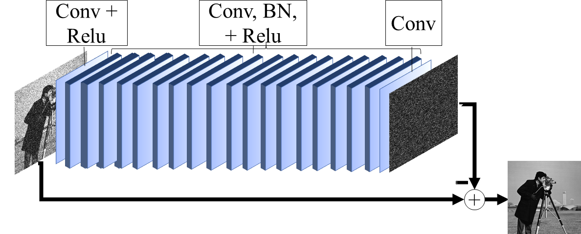
Figure 2: Network architecture of the DnCNN denoiser. Note that it takes advantage of residual learning.

The prRED framework can incorporate nearly any denoising algorithm. We call the special case of prRED with the DnCNN denoiser “prDeep”.

DnCNN (Zhang et al., 2017) is a state-of-the-art denoiser for removing additive white Gaussian noise from natural images. DnCNN consists of 16 to 20 convolutional layers of size $3\times 3$ (we used 20). Sandwiched between these layers are ReLU (Krizhevsky et al., 2012) and batch-normalization (Ioffe & Szegedy, 2015) operations. DnCNN is trained using residual learning (He et al., 2016).

In practice, DnCNN noticeably outperforms the popular BM3D algorithm. Moreover, thanks to parallelization and GPU computing, it runs hundreds of times faster than BM3D.

We trained four DnCNN networks at different noise levels. To train, we loosely followed the procedure outlined in (Zhang et al., 2017). In particular, we trained with 300 000 overlapping patches drawn from $400$ images in the Berkeley Segmentation Dataset (Martin et al., 2001). For each image patch, we added additive white Gaussian noise with a standard deviation of either $60$, $40$, $20$, or $10$. where our images had a dynamic range of $[0,255]$. We then setup DnCNN to recover the noise-free image. We used the mean-squared error between the noise-free ground truth image and our denoised reconstructions as the cost function. We trained the network with stochastic gradient descent and the ADAM optimizer (Kingma & Ba, 2014) with a batch size of 256. Our training rate was $0.001$, which we dropped to $0.0001$ and then $0.00001$ when the validation error stopped improving. Training took just over 3 hours per noise level on an Nvidia Pascal Titan X.

4 Experimental Results

In this section we compare prDeep to several other PR algorithms on simulated data with varying amounts of Poisson noise. We test the algorithms with both coded diffraction pattern (CDP) and Fourier measurements. In both sets of tests, we sample and reconstruct 6 “natural” and 6 “unnatural” (real and nonnegative) test images, which are presented in Figures 3 and 4.

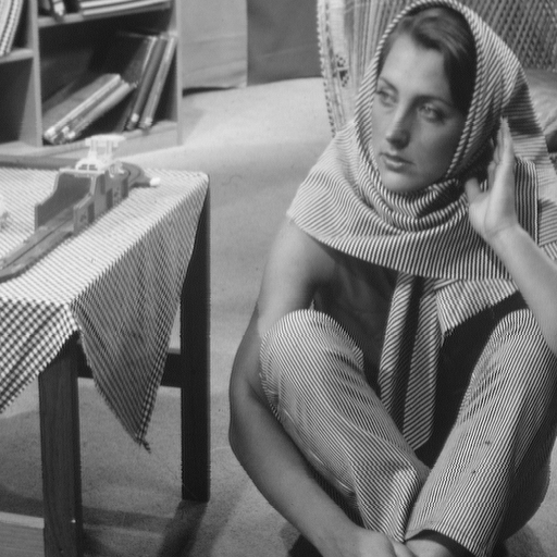
(a) Barbara

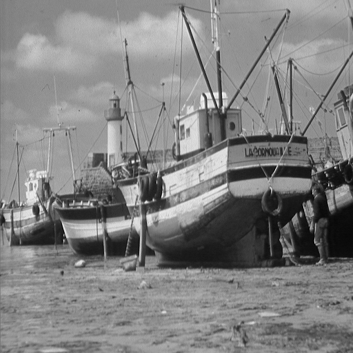
(b) Boat

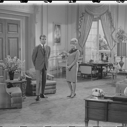
(c) Couple

(d) Peppers

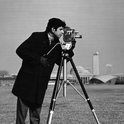
(e) Cameraman

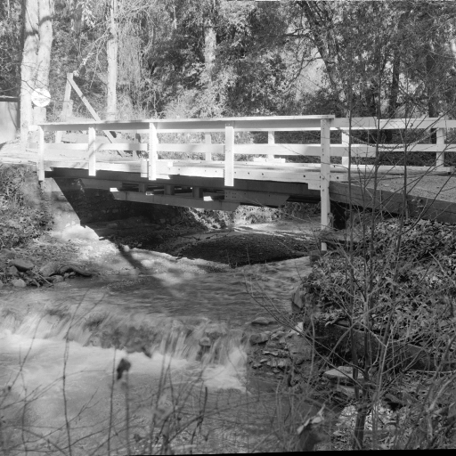
(f) Bridge

Figure 3: The six “natural” test images. They follow a distribution very similar to the training data.

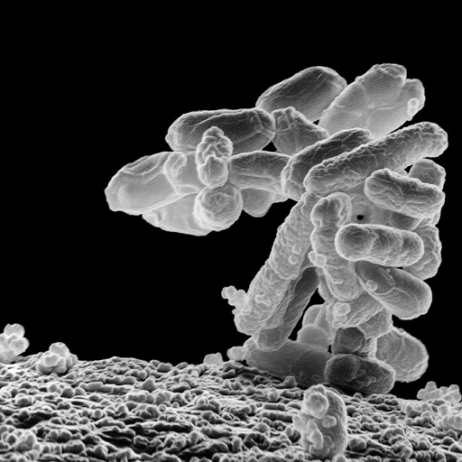
(a) E. Coli

(b) Yeast

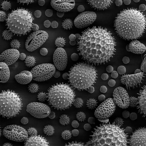
(c) Pollen

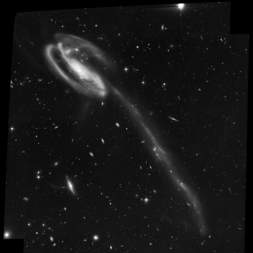
(d) Tadpole Galaxy

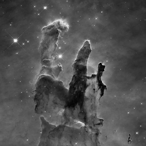
(e) Pillars of Creation

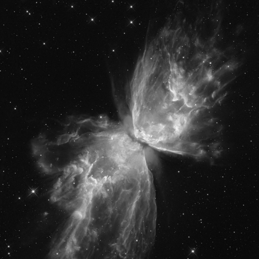
(f) Butterfly Nebula

Figure 4: The six “unnatural” test images. They follow a distribution distinct from the training data. Images are from Wikipedia and follow public domain licenses.

4.1 Experimental Setup

Competing Algorithms.

We compare prDeep against Hybrid Input-Output (HIO) (Fienup, 1982), Oversampling Smoothness (OSS) (Rodriguez et al., 2013), Wirtinger Flow (WF) (Candes et al., 2015a), DOLPHIn (Tillmann et al., 2016), SPAR (Katkovnik & Astola, 2012; Katkovnik, 2017), and BM3D-prGAMP (Metzler et al., 2016b). We also compare with Plug-and-Play ADMM (Venkatakrishnan et al., 2013; Heide et al., 2016) using both the BM3D and DnCNN denoisers. HIO and WF are baseline algorithms designed for Fourier and CDP measurements, respectively. OSS is an alternating projection algorithm designed for noisy Fourier measurements. It imposes a smoothness constraint to regions outside of the target’s support. DOLPHIn is an iterative PR algorithm designed to reconstruct images from noisy CDP measurements. It imposes a sparsity constraint with respect to a learned dictionary. SPAR, BM3D-prGAMP, and Plug-and-Play ADMM were described in Section 2.2.

Table 1: PSNRs and run times (sec) of $128\times 128$ reconstructions with four intensity-only CDP measurements and varying amounts of Poisson noise.

	$\alpha=9$			$\alpha=27$			$\alpha=81$
	PSNR Natural	PSNR Unnatural	Time	PSNR Natural	PSNR Unnatural	Time	PSNR Natural	PSNR Unnatural	Time
HIO	36.1	36.0	4.2	26.1	26.0	5.9	14.8	16.9	5.9
WF	34.3	34.2	0.8	24.7	24.0	0.9	13.2	13.0	6.7
DOLPHIn	31.0	28.8	1.1	27.9	26.9	1.1	17.9	20.8	1.1
SPAR	34.4	36.0	15.7	29.4	31.1	15.7	24.5	26.4	15.7
BM3D-prGAMP	34.1	35.4	17.2	31.4	32.2	17.7	22.5	22.3	23.1
BM3D-ADMM	38.5	39.0	51.6	31.9	33.4	40.0	24.4	26.9	37.7
DnCNN-ADMM	39.9	40.6	17.1	32.6	33.4	9.8	21.6	22.7	7.9
prDeep	39.1	40.1	25.4	32.8	34.0	23.2	20.9	24.5	23.1

Table 2: PSNRs and run times (sec) of $128\times 128$ reconstructions with $4\times$ over-sampled intensity-only Fourier measurements and varying amounts of Poisson noise.

	$\alpha=2$			$\alpha=3$			$\alpha=4$
	PSNR Natural	PSNR Unnatural	Time	PSNR Natural	PSNR Unnatural	Time	PSNR Natural	PSNR Unnatural	Time
HIO	22.2	20.8	10.6	19.9	17.9	10.4	17.9	15.5	10.7
WF	15.2	18.8	6.7	15.1	18.5	6.6	15.2	18.5	6.7
OSS	18.6	23.8	18.3	18.4	23.1	18.6	18.6	22.7	18.1
SPAR	22.0	23.9	79.1	19.6	22.6	77.0	19.4	20.5	83.0
BM3D-prGAMP	24.5	26.0	84.3	23.2	24.4	82.8	21.0	22.7	84.4
BM3D-ADMM	27.5	28.3	155.7	24.5	25.0	156.8	21.8	23.1	156.8
DnCNN-ADMM	29.3	31.3	65.0	26.0	25.8	62.4	22.0	23.4	64.0
prDeep	28.4	30.6	105.1	28.5	26.4	105.0	26.4	25.1	107.1

Implementation.

All algorithms were tested using Matlab 2017a on a desktop PC with an Intel 6800K CPU and an Nvidia Pascal Titan X GPU. Dolphin, SPAR, and BM3D-prGAMP used their respective authors’ implementations. We created our own version of Plug and Play ADMM based off of code original developed in (Chan et al., 2017). We use FASTA to solve the nonlinear least squares problem at each iteration of the algorithm. prDeep and DnCNN-ADMM used a MatConvNet (Vedaldi & Lenc, 2015) implementation of DnCNN. A public implementations of prDeep is available at https://github.com/ricedsp/prDeep.

Measurement and Noise Model.

Model mismatch and Poisson shot noise are the dominant sources of noise in many PR applications (Yeh et al., 2015). In this paper, we focus on shot noise, which we approximate as

$$y^{2}=|z|^{2}+w\text{ with }w\sim N(0,\alpha^{2}\text{Diag}(|z|^{2})),$$

where $z=\mathbf{A}x$ with known $\mathbf{A}$, and where $\text{Diag}(|z|^{2})$ is a diagonal matrix with diagonal elements $|z|^{2}$.

Some algebra and the central limit theorem can be used to show that $y^{2}/\alpha^{2}\sim\text{Poisson}((|z|/\alpha)^{2})$. In effect, $y^{2}$ is a rescaled Poisson random variable. The term $\alpha$ controls the variance of the random variable and thus the effective signal-to-noise ratio in our problem.

Parameter Tuning.

HIO was run for $1000$ iterations. WF was run for $2000$ iterations. BM3D-prGAMP was run for $50$ iterations. prDeep was run for $200$ iterations four times; once for each of the denoisers networks (trained at standard deviations $60$, $40$, $20$, and $10$). The result from reconstructing with the first denoiser was used to warm-start reconstructing with the second, the second warm-started the third, etc. Plug and Play ADMM was similarly run for $50$ iterations four times. ADMM converged faster than prDeep and did not benefit from additional iterations.

SPAR reconstructed $x$ using $y^{2}/\alpha^{2}$ rather than $y$, as its loss function expects Poisson distributed random variables. prDeep’s parameter $\lambda$, which determines the amount of regularization, was set to $\bar{\sigma}_{w}$ when dealing with Fourier measurements and $0.1\bar{\sigma}_{w}$ when dealing with CDP measurements, where $\bar{\sigma}_{w}^{2}$ denotes the sample variance of the noise. The parameter in ADMM analogues to $\lambda$ was set to $.2\bar{\sigma}_{w}$ when dealing with Fourier measurements and $0.02\bar{\sigma}_{w}$ when dealing with CDP measurements. The algorithms otherwise used their default parameters.

Initialization.

With oversampled CDP measurements of real-valued signals, none of the algorithms were particularly sensitive to initialization; initializing with a vector of ones worked sufficiently well. In contrast, with Fourier measurements, the algorithms were very sensitive to initialization. We experimented with various spectral initializers, but found they were ineffective with (noisy and only $4\times$ oversampled) Fourier measurements. Instead, we first ran the HIO algorithm (for $50$ iterations) $50$ times, from random initializations, to form 50 estimates of the signal: $\widehat{x}_{1}$, $\widehat{x}_{2}$, … $\widehat{x}_{50}$. We then used the reconstruction $\widehat{x}_{i}$ with the lowest residual ($\|y-|\mathbf{A}\widehat{x}_{i}|\|_{2}$) as an initialization for HIO. HIO was then run for $1000$ iterations, and the result was used to initialize the other algorithms. This process was repeated three times and the reconstruction with the smallest residual was used as the final estimate. The reported computation times (for Fourier measurements) include the time required to initialize the algorithms and run them three times.

4.2 Simulated Coded Diffraction Measurements

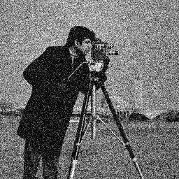
(a) HIO (21 sec)

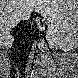
(b) WF (24 sec)

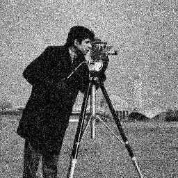
(c) DOLPHIn (3 sec)

(d) SPAR (58 sec)

(e) BM3D-prGAMP (91 sec)

(f) BM3D-ADMM (153 sec)

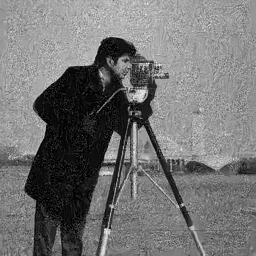
(g) DnCNN-ADMM (25 sec)

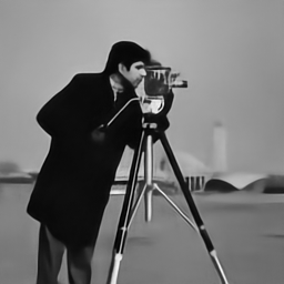
(h) prDeep (72 sec)

Figure 5: Reconstructions of $256\times 256$ image from four noisy intensity-only CDP measurements ($\alpha=81$) with several PR algorithms. All five plug-and-play methods provide similar reconstructions.

We first test the algorithms with CDP intensity-only measurements. CDP is a measurement model proposed in (Candes et al., 2015b) that uses a spatial light modulator (SLM) to spread a target’s frequency information and make it easier to reconstruct. Under a CDP measurement model, the target is illuminated by a coherent source and then has its phase immediately modulated by a known random pattern using an SLM. The complex field then undergoes far-field Fraunhofer diffraction, which can be modeled by a 2D Fourier transform, before its intensity is recorded by a standard camera. Multiple measurements, with different random SLM patterns, are recorded. In this work, we model the capture of four measurements using a phase-only SLM. Mathematically, our measurement operator is as follows

$$\mathbf{A}=\left[\begin{array}[]{ll}\mathbf{F}\mathbf{D_{1}}\\ \mathbf{F}\mathbf{D_{2}}\\ \mathbf{F}\mathbf{D_{3}}\\ \mathbf{F}\mathbf{D_{4}}\end{array}\right],$$ (13)

where $\mathbf{F}$ represents the 2D Fourier transform and $\mathbf{D}_{1}$, $\mathbf{D}_{2}$, … are diagonal matrices with nonzero elements drawn uniformly from the unit circle in the complex plane.

In Table 1 we compare the performance of the various PR algorithms. We do not include a comparison with OSS as it is setup specifically for Fourier measurements. We report recovery accuracy in terms of mean peak-signal-to-noise ratio (PSNR) across two sets of test images. We report run time in seconds.

Table 1 demonstrates that, when dealing with CDP measurements at low SNRs (large $\alpha$), all five plug-and-play methods produce similar reconstructions.

In Figure 5, we visually compare the reconstructions of a $256\times 256$ image using the algorithms under test. With CDP measurements, all of the plug-and-play algorithms do a good job reconstructing the signal from noisy measurements.

4.3 Simulated Fourier Measurements

(a) HIO (40 sec)

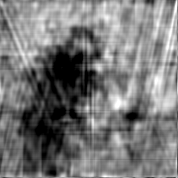
(b) WF (63 sec)

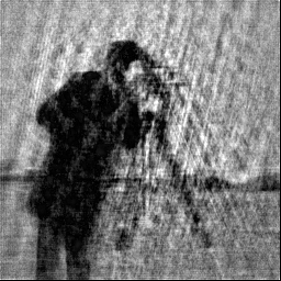
(c) OSS (65 sec)

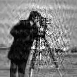
(d) SPAR (294 sec)

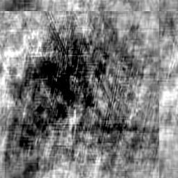
(e) BM3D-prGAMP (306 sec)

(f) BM3D-ADMM (576 sec)

(g) DnCNN-ADMM (426 sec)

(h) prDeep (345 sec)

Figure 6: Reconstructions of $256\times 256$ image from noisy $4\times$ oversampled intensity-only Fourier measurements ($\alpha=3$) with several PR algorithms. Plug and Play ADMM and prDeep provide the best reconstructions.

Fourier measurements of real-valued signals are prevalent in many real-world applications. Many PR applications exploit the Fourier-transform property $\mathbf{F}(x\star x)=|\mathbf{F}x|^{2}$, where $\star$ denotes correlation. This implies that in applications where one can measure or estimate the autocorrelation function of an object one can also measure the modulus squared of its Fourier transform. This allows PR algorithms to reconstruct the object.

This relationship has been used in multiple contexts. In astronomical imaging, this relationship has been used to image through turbulent atmosphere (Dainty & Fienup, 1987). In laser-illuminated imaging, this relationship has been used to reconstruct diffuse objects without speckle noise (Fienup & Idell, 1988). More recently, this relationship has been used to image through random scattering media, such as biological tissue (Katz et al., 2014). In all of these applications, one reconstructs the real-valued intensity distribution of the object.

In these tests we oversampled the spectrum by $4\times$. That is, we first placed $128\times 128$ images at the center of a $256\times 256$ square and then took the 2D Fourier transform. We assumed that the support, i.e., the location of the image within the $256\times 256$ grid, was known a priori.

Table 2 compares the reconstruction accuracies and recovery times of several PR algorithms. We do not include results for DOLPHIn, as it completely failed with Fourier measurements. Note that, at a given noise level, the reconstructions from Fourier measurements are far less accurate than their CDP counterpart. Table 2 demonstrates that with Fourier measurements and large amounts of noise prDeep is superior to existing PR algorithms.

In Figure 6, we again visually compare the reconstructions from the algorithms under test, this time with Fourier measurements. In this regime prDeep produces fewer artifacts than competing methods.

5 Conclusions and Future Work

In this paper, we have extended and applied the Regularization by Denoising (RED) framework to the problem of PR. Our new algorithm, prDeep, is exceptionally robust to noise thanks to the use of the DnCNN image denoising neural network. As we demonstrated in our experiments, prDeep is also able to handle a wide range of measurement matrices, from intensity-only coded diffraction patterns to Fourier measurements.

By integrating a neural network into a traditional optimization algorithm, prDeep inherits the strengths of both optimization and deep-learning. Like other optimization-based algorithms, prDeep is flexible and can be applied to PR problems with different measurement models, noise levels, etc., without having to undergo costly retraining. Like other deep-learning-based techniques, for any given problem prDeep can take advantage of powerful learned priors and outperform traditional, hand-designed methods.

prDeep is not a purely academic PR algorithm; it can handle Fourier measurements of real-valued signals, a measurement model that plays a key role in many imaging applications. However, prDeep does have a major limitation; it is presently restricted to amplitude-only targets. Extending prDeep to handle complex-valued targets is a promising and important direction for future research.

Acknowledgements

Phil Schniter was supported by NSF grants CCF-1527162 and CCF-1716388. Richard Baraniuk, Ashok Veeraraghavan, and Chris Metzler were supported by the DOD Vannevar Bush Faculty Fellowship N00014-18-1-2047, NSF Career– IIS-1652633, and the NSF GRF program, respectively. They were also supported by NSF grant CCF-1527501, ARO grant W911NF-15-1-0316, AFOSR grant FA9550-14-1-0088, ONR grant N00014-17-1-2551, DARPA REVEAL grant HR0011-16-C-0028, ARO grant Supp-W911NF-12-1-0407, and an ONR BRC grant for Randomized Numerical Linear Algebra.

References

- Bahmani & Romberg (2017) Bahmani, S. and Romberg, J. Phase retrieval meets statistical learning theory: A flexible convex relaxation. In Artificial Intelligence and Statistics, pp. 252–260, 2017.
- Boominathan & Mitra (2018) Boominathan, L. and Mitra, K. Phase retrieval under reduced measurements for fourier ptychography using conditional adversarial networks. Unpublished manuscript, 2018.
- Candes et al. (2013) Candes, E., Strohmer, T., and Voroninski, V. Phaselift: Exact and stable signal recovery from magnitude measurements via convex programming. Communications on Pure and Applied Mathematics, 66(8):1241–1274, 2013.
- Candes et al. (2015a) Candes, E., Li, X., and Soltanolkotabi, M. Phase retrieval via wirtinger flow: Theory and algorithms. IEEE Transactions on Information Theory, 61(4):1985–2007, 2015a.
- Candes et al. (2015b) Candes, E., Li, X., and Soltanolkotabi, M. Phase retrieval from coded diffraction patterns. Applied and Computational Harmonic Analysis, 39(2):277–299, 2015b.
- Chan et al. (2017) Chan, S. H., Wang, X., and Elgendy, O. A. Plug-and-play admm for image restoration: Fixed-point convergence and applications. IEEE Transactions on Computational Imaging, 3(1):84–98, 2017.
- Chandra et al. (2017) Chandra, R., Studer, C., and Goldstein, T. Phasepack: A phase retrieval library. arXiv preprint arXiv:1711.10175, 2017.
- Chang et al. (2017) Chang, J., Li, C., Póczos, B., Kumar, B., and Sankaranarayanan, A. One network to solve them all; solving linear inverse problems using deep projection models. In 2017 IEEE International Conference on Computer Vision (ICCV), pp. 5889–5898, Oct 2017.
- Chen & Candes (2015) Chen, Y. and Candes, E. Solving random quadratic systems of equations is nearly as easy as solving linear systems. In Advances in Neural Information Processing Systems, pp. 739–747, 2015.
- Dabov et al. (2007) Dabov, K., Foi, A., Katkovnik, V., and Egiazarian, K. Image denoising by sparse 3-d transform-domain collaborative filtering. IEEE Transactions on Image Processing, 16(8):2080–2095, 2007.
- Dainty & Fienup (1987) Dainty, C. and Fienup, J. Phase retrieval and image reconstruction for astronomy. Image Recovery: Theory and Application, 231:275, 1987.
- Danielyan et al. (2010) Danielyan, A., Foi, A., Katkovnik, V., Egiazarian, K., and Milanfar, P. Spatially adaptive filtering as regularization in inverse imaging: Compressive sensing super-resolution and upsampling. Super-Resolution Imaging, pp. 123–154, 2010.
- Diamond et al. (2017) Diamond, S., Sitzmann, V., Heide, F., and Wetzstein, G. Unrolled optimization with deep priors. arXiv preprint arXiv:1705.08041, 2017.
- Dong et al. (2014) Dong, C., Loy, C., He, K., and Tang, X. Learning a deep convolutional network for image super-resolution. In European Conference on Computer Vision, pp. 184–199. Springer, 2014.
- Donoho et al. (2009) Donoho, D., Maleki, A., and Montanari, A. Message-passing algorithms for compressed sensing. Proceedings of the National Academy of Sciences, 106(45):18914–18919, 2009.
- Fienup (1978) Fienup, J. Reconstruction of an object from the modulus of its fourier transform. Optics letters, 3(1):27–29, 1978.
- Fienup (1982) Fienup, J. Phase retrieval algorithms: a comparison. Applied optics, 21(15):2758–2769, 1982.
- Fienup & Idell (1988) Fienup, J. and Idell, P. Imaging correlography with sparse arrays of detectors. Optical Engineering, 27(9):279778, 1988.
- Gerchberg (1972) Gerchberg, R. A practical algorithm for the determination of phase from image and diffraction plane pictures. Optik, 35:237, 1972.
- Goldstein & Studer (2016) Goldstein, T. and Studer, C. Phasemax: Convex phase retrieval via basis pursuit. arXiv preprint arXiv:1610.07531, 2016.
- Goldstein et al. (2014) Goldstein, T., Studer, C., and Baraniuk, R. A field guide to forward-backward splitting with a fasta implementation. arXiv preprint arXiv:1411.3406, 2014.
- Goodman (2005) Goodman, J. Introduction to Fourier optics. Roberts and Company Publishers, 2005.
- Gregor & LeCun (2010) Gregor, K. and LeCun, Y. Learning fast approximations of sparse coding. In Proceedings of the 27th International Conference on International Conference on Machine Learning, pp. 399–406. Omnipress, 2010.
- Griffin & Lim (1984) Griffin, D. and Lim, J. Signal estimation from modified short-time fourier transform. Acoustics, Speech and Signal Processing, IEEE Transactions on, 32(2):236–243, 1984.
- He et al. (2016) He, K., Zhang, X., Ren, S., and Sun, J. Deep residual learning for image recognition. Proc. IEEE Int. Conf. Comp. Vision, and Pattern Recognition, pp. 770–778, 2016.
- Heide et al. (2014) Heide, F., Steinberger, M., Tsai, Y., Rouf, M., Pajak, D., Reddy, D., Gallo, O., Liu, J., Heidrich, W., Egiazarian, K., et al. Flexisp: A flexible camera image processing framework. ACM Transactions on Graphics (TOG), 33(6):231, 2014.
- Heide et al. (2016) Heide, F., Diamond, S., Nießner, M., Ragan-Kelley, J., Heidrich, W., and Wetzstein, G. Proximal: Efficient image optimization using proximal algorithms. ACM Transactions on Graphics (TOG), 35(4):84, 2016.
- Ioffe & Szegedy (2015) Ioffe, S. and Szegedy, C. Batch normalization: Accelerating deep network training by reducing internal covariate shift. arXiv preprint arXiv:1502.03167, 2015.
- Kappeler et al. (2017) Kappeler, A., Ghosh, S., Holloway, J., Cossairt, O., and Katsaggelos, A. Ptychnet: CNN based fourier ptychography. In Image Processing (ICIP), 2017 IEEE International Conference on. IEEE, 2017.
- Katkovnik (2017) Katkovnik, V. Phase retrieval from noisy data based on sparse approximation of object phase and amplitude. arXiv preprint arXiv:1709.01071, 2017.
- Katkovnik & Astola (2012) Katkovnik, V. and Astola, J. Phase retrieval via spatial light modulator phase modulation in 4f optical setup: numerical inverse imaging with sparse regularization for phase and amplitude. JOSA A, 29(1):105–116, 2012.
- Katz et al. (2014) Katz, O., Heidmann, P., Fink, M., and Gigan, S. Non-invasive single-shot imaging through scattering layers and around corners via speckle correlations. Nature Photonics, 8(10):784–790, 2014.
- Kingma & Ba (2014) Kingma, D. and Ba, J. Adam: A method for stochastic optimization. arXiv preprint arXiv:1412.6980, 2014.
- Krizhevsky et al. (2012) Krizhevsky, A., Sutskever, I., and Hinton, G. Imagenet classification with deep convolutional neural networks. Proc. Adv. in Neural Processing Systems (NIPS), pp. 1097–1105, 2012.
- Martin et al. (2001) Martin, D., Fowlkes, C., Tal, D., and Malik, J. A database of human segmented natural images and its application to evaluating segmentation algorithms and measuring ecological statistics. Proc. Int. Conf. Computer Vision, 2:416–423, July 2001.
- Metzler et al. (2016a) Metzler, C., Maleki, A., and Baraniuk, R. From denoising to compressed sensing. IEEE Transactions on Information Theory, 62(9):5117–5144, 2016a.
- Metzler et al. (2016b) Metzler, C., Maleki, A., and Baraniuk, R. BM3D-PRGAMP: Compressive phase retrieval based on BM3D denoising. In 2016 IEEE International Conference on Image Processing (ICIP), pp. 2504–2508. IEEE, 2016b.
- Metzler et al. (2017a) Metzler, C., Mousavi, A., and Baraniuk, R. Learned d-amp: Principled neural network based compressive image recovery. In Advances in Neural Information Processing Systems, pp. 1770–1781, 2017a.
- Metzler et al. (2017b) Metzler, C., Sharma, M., Nagesh, S., Baraniuk, R., Cossairt, O., and Veeraraghavan, A. Coherent inverse scattering via transmission matrices: Efficient phase retrieval algorithms and a public dataset. In 2017 IEEE International Conference on Computational Photography (ICCP), pp. 1–16. IEEE, 2017b.
- Millane (1990) Millane, R. Phase retrieval in crystallography and optics. JOSA A, 7(3):394–411, 1990.
- Moravec et al. (2007) Moravec, M. L., Romberg, J. K., and Baraniuk, R. G. Compressive phase retrieval. In Optical Engineering+ Applications, pp. 670120–670120. International Society for Optics and Photonics, 2007.
- Pfeifer et al. (2006) Pfeifer, M., Williams, G., Vartanyants, I., Harder, R., and Robinson, I. Three-dimensional mapping of a deformation field inside a nanocrystal. Nature, 442(7098):63–66, 2006.
- Rangan (2011) Rangan, S. Generalized approximate message passing for estimation with random linear mixing. In Information Theory Proceedings (ISIT), 2011 IEEE International Symposium on, pp. 2168–2172. IEEE, 2011.
- Rivenson et al. (2017) Rivenson, Y., Zhang, Y., Gunaydin, H., Teng, D., and Ozcan, A. Phase recovery and holographic image reconstruction using deep learning in neural networks. arXiv preprint arXiv:1705.04286, 2017.
- Rodriguez et al. (2013) Rodriguez, J., Xu, R., Chen, C., Zou, Y., and Miao, J. Oversampling smoothness: an effective algorithm for phase retrieval of noisy diffraction intensities. Journal of applied crystallography, 46(2):312–318, 2013.
- Romano et al. (2017) Romano, Y., Elad, M., and Milanfar, P. The little engine that could: Regularization by denoising (red). SIAM Journal on Imaging Sciences, 10(4):1804–1844, 2017.
- Schniter & Rangan (2015) Schniter, P. and Rangan, S. Compressive phase retrieval via generalized approximate message passing. IEEE Transactions on Signal Processing, 63(4):1043–1055, 2015.
- Schniter et al. (2016) Schniter, P., Rangan, S., and Fletcher, A. Denoising based vector approximate message passing. arXiv preprint arXiv:1611.01376, 2016.
- Tillmann et al. (2016) Tillmann, A., Eldar, Y., and Mairal, J. Dolphin-dictionary learning for phase retrieval. IEEE Transactions on Signal Processing, 64(24):6485–6500, 2016.
- Vedaldi & Lenc (2015) Vedaldi, A. and Lenc, K. Matconvnet – Convolutional neural networks for MATLAB. Proc. ACM Int. Conf. on Multimedia, 2015.
- Venkatakrishnan et al. (2013) Venkatakrishnan, S., Bouman, C., and Wohlberg, B. Plug-and-play priors for model based reconstruction. In Global Conference on Signal and Information Processing (GlobalSIP), 2013 IEEE, pp. 945–948. IEEE, 2013.
- Yeh et al. (2015) Yeh, L., Dong, J., Zhong, J., Tian, L., Chen, M., Tang, G., Soltanolkotabi, M., and Waller, L. Experimental robustness of fourier ptychography phase retrieval algorithms. Optics express, 23(26):33214–33240, 2015.
- Zhang et al. (2017) Zhang, K., Zuo, W., Chen, Y., Meng, D., and Zhang, L. Beyond a gaussian denoiser: Residual learning of deep cnn for image denoising. IEEE Transactions on Image Processing, 26(7):3142–3155, 2017.
- Zheng & Yang (2013) Zheng, G.and Horstmeyer, R. and Yang, C. Wide-field, high-resolution fourier ptychographic microscopy. Nature Photonics, 7(9):739–745, 2013.