Composite Difference-Max Programs for Modern Statistical Estimation Problems

Abstract

Many modern statistical estimation problems are defined by three major components: a statistical model that postulates the dependence of an output variable on the input features; a loss function measuring the error between the observed output and the model predicted output; and a regularizer that controls the overfitting and/or variable selection in the model. We study the sampling version of this generic statistical estimation problem where the model parameters are estimated by empirical risk minimization, which involves the minimization of the empirical average of the loss function at the data points weighted by the model regularizer. In our setup we allow all three component functions discussed above to be of the difference-of-convex (dc) type and illustrate them with a host of commonly used examples, including those in continuous piecewise affine regression and in deep learning (where the activation functions are piecewise affine). We describe a nonmonotone majorization-minimization (MM) algorithm for solving the unified nonconvex, nondifferentiable optimization problem which is formulated as a specially structured composite dc program of the pointwise max type, and present convergence results to a directional stationary solution. An efficient semismooth Newton method is proposed to solve the dual of the MM subproblems. Numerical results are presented to demonstrate the effectiveness of the proposed algorithm and the superiority of continuous piecewise affine regression over the standard linear model.

62J02, 90C26, 49J52

1 Introduction

Many modern statistical estimation problems are defined by three major components: a statistical model that postulates the dependence of an output quantity on the input features; a loss function measuring the error between the observed output and model predicted output; and a regularizer that controls the overfitting and/or variable selection in the model. The overall estimation problem is to determine certain unknown parameters in the statistical model. In practical computation, samples on the underlying covariates (inputs) and output are available and a data-based empirical objective combined with a regularizer is formulated as a minimization problem that constitutes the workhorse of the estimation process. This paper addresses the computational solution of the latter optimization problem which is challenged by its nonconvexity and nondifferentiability. These features immediately raise the question about the stationarity, let alone minimizing, properties of the computed solution by an iterative algorithm. Our goal is to compute a directional stationary solution [47], which is the sharpest kind among all stationary solutions.

Traditionally, a statistical model is usually described by a linear combination of the input features, resulting in a linear regression or classification model. Nevertheless, in recent years, research into the use of piecewise affine, convex [19, 20, 39] and nonconvex [24] estimation functions has been on the rise. There are other piecewise affine/quadratic functions that arise from different applications, such as those using piecewise affine functions to approximate the signum function and multi-layer neural networks in deep learning [61, Chapter 4]. These nontraditional, nondifferentiable estimation functions have provided an important impetus for our work.

Some classical convex loss measures are based on the absolute-value or squared errors between the model predicted outputs and the observed outputs, leading to a $\ell_{1}$ or $\ell_{2}$ loss function for regression. Other loss functions include a logarithmic loss for logistic regression, and an exponential loss for boosting. In the area of support vector machines, a hinge loss is commonly used for binary classification. In recent years, a truncated hinge loss function has been proposed to reduce the effect of outliers [64]. A distinguished property of the latter loss function is that it is nonconvex and nondifferentiable. All these loss measures are composed with the statistical model involving the parameters to be estimated, leading to an overall composite loss function to be minimized, which is nonconvex and nondifferentiable, due either to a piecewise statistical model or a loss function that lacks convexity and/or differentiability. In the area of support vector machines and other applications, a norm function of the model variables is often used as the model regularizer to avoid overfitting. In recent years, sparsity constraints to avoid model overfitting [26] is an important consideration in high-dimensional statistical learning. Starting with the pioneering work of Fan and Li [22], various sparsity functions have been proposed as surrogates of the discontinuous counting step function; it was shown in [1, 34] that all these surrogate sparsity functions can be expressed as the difference of two convex functions of a particular type.

In this paper, we introduce a composite difference-of-convex-piecewise program of the pointwise max type as a unification of a host of statistical models, loss functions, and model regularizers. A highlight of this formulation is the emphasis on the separate roles of each component function that is key to the development of a nonmonotone majorization-minimization (MM) algorithm for solving the overall nonconvex, nondifferentiable optimization problem. While global optima of nonconvex problems cannot be computed, stationary solutions of various kinds are computable by iterative algorithms with guaranteed convergence. What is essential is that focus should be placed on computing sharp stationary solutions which distinguish themselves as being the ones that must satisfy all other relaxed definitions of stationarity. With guaranteed subsequential convergence, the developed MM algorithm aims to compute such a stationary point that is based on the elementary notion of directional derivatives of the objective function. By using the Kurdyka-Łojaziewicz (KL) theory of semi-analytic functions [2, 3, 9], we also show the sequential convergence of the iterates produced by the algorithm. In order to handle the nondifferentiable pointwise max terms, auxiliary variables are employed to express these pointwise maximum functions as constraints. With the regularization of the added variables in defining the subproblems, the resulting MM algorithm no longer guarantees the monotone property of the original objective; this leads to our terminology of “nonmonotone MM algorithm”. Due to the modifications which are introduced to facilitate the fast and efficient solution of the subproblems in the iterative steps, a separate proof of convergence is needed for the algorithm. To ensure the rapid convergence and high-accuracy required of the solution of the subproblems, we employ the semismooth Newton method (SN) [50, 46] for semismoothly differentiable (SC¹) functions applied to the dual of such subproblems. We present numerical results to demonstrate the effectiveness of the overall algorithm and the superiority of a nontraditional continuous piecewise affine regression model over the traditional linear model using least-squares regression. In addition to this specific problem, the nonmonotone MM algorithm combined with the SN method (abbreviated as MM+SN) developed in this paper has wide applications to many related problems that include the multi-layer neural network problems with piecewise activation functions in deep learning. Due to page limit, we will report the details of the other applications in separate papers.

The major contributions of this paper are fourfold: (a) we identify a unified composite difference-max program for a host of modern statistical estimation problems and illustrate the formulation with a variety of special instances; (b) we develop a majorization-minimization based algorithm for computing, for the first time, a directional stationary solution of such a nonconvex, nonsmooth program; (c) we present a semismooth Newton method for solving the MM subproblems and illustrate its effectiveness when applied to a piecewise affine regression problem; and (d) we report computational results on the latter application that demonstrate the superiority of this nontraditional statistical estimation approach over traditional linear regression.

2 A Unified Composite Difference-Convex-Piecewise Program

In the definition of a statistical estimation problem, we place particular emphasis and care on the mathematical properties of its defining functions; identifying these properties is needed to effectively deal with the joint feature of nonconvexity and nondifferentiability and to facilitate the design of the MM+SN algorithm and its analysis for solving the resulting optimization problem. Specifically, the optimization problem consists of the following four major components, each playing a separate role in the overall statistical estimation process. As such, distinguishing them offers flexibility to accommodate a variety of model specifications.

$\bullet$ A parametric statistical model: $y=\psi(x;\theta)+\varepsilon$, where $y$ is the response (output) variable (taken to be a scalar) given the input $x\in\mathbb{R}^{d}$, $\varepsilon$ is the unobserved random error assumed to have (conditional) mean zero, and $\theta\in\mathbb{R}^{m}$ is the model parameter to be estimated, for some positive integers $d$ (number of input features) and $m$ (number of parameters). In general, these two dimensions, $d$ and $m$, may be different (see e.g. (3)); however, they may be the same as in the case of linear regression.

$\bullet$ An output-dependent loss function $\varphi(y,\bullet)$, whose composition with the statistical model $\psi(x;\theta)$ leads to the composite function $(\theta;y,x)\mapsto\varphi(y,\psi(x;\theta))$ that provides a measure of the deviation between the model predicted output $\psi(x;\theta)$ and the observed response $y$; we stress the importance of this composition as properties of $\varphi$ and $\psi$ may be very different and need to be understood separately for best results.

$\bullet$ A regularizing function $P(\theta)$ that is used either for the purpose of strongly convexifying the objective function or in high-dimensional problems to control the selection of the model parameter $\theta$; the latter control is particularly important to avoid overfitting when the number of features $d$ is relatively large.

$\bullet$ An admissible set $\Theta\subseteq\mathbb{R}^{m}$ that further restricts the parameter space in the presence of domain knowledge on the parameter $\theta$; often this set $\Theta$ is the whole space $\mathbb{R}^{m}$, leading to an unconstrained selection of the parameter.

Together, the tuple $(\varphi,\psi,\Theta)$ defines the following constrained minimization problem that is central to many statistical estimation problems:

(1) $${\operatornamewithlimits{\mbox{minimize}}_{\theta\,\in\,\Theta}}\ {\rm I\!E}\left[\,\varphi(y,\psi(x;\theta))\,\right],$$

where the expectation $\mathbb{E}$ is taken over the joint distribution of the input $x$ and the output $y$. The objective expresses the average loss of accuracy in the model output versus the realized output taking into account the uncertainties in the random input-output pair $(x,y)$. This perspective of statistical estimation is in line with stochastic programming and is a departure from classical statistical estimation where there is always a postulate of a “ground truth” of the estimator. In this paper, we investigate the numerical solution of problem (1) via the application of the sample average approximation (SAA) scheme. Specifically, taking $N$ independent and identically distributed samples $\{(x^{s},y_{s})\}_{s=1}^{N}\subseteq\mathbb{R}^{d+1}$ and adding the regularizer $P(\theta)$ weighted by the scalar $\gamma_{N}\geq 0$, we consider the empirical optimization problem:

(2) $${\operatornamewithlimits{\mbox{minimize}}_{\theta\,\in\,\Theta}}\ \displaystyle{\frac{1}{N}}\,\displaystyle{\sum_{s=1}^{N}}\,\left[\,\varphi(y_{s},\psi(x^{s};\theta))\,\right]+\gamma_{N}\,P(\theta).$$

While this formulation (2) is rather classical, the detailed treatment of the distinguished properties of the functions $(\varphi,\psi,P)$ constitutes the novelty and intellectual merits of the present paper. In what follows, we present some details of these functions and describe how they arise. An important point of the discussion is to motivate a focused formulation of problem (2) that allows a unified treatment of these statistical estimation problems as a composite diff-max program by a common algorithmic procedure with guaranteed convergence properties; see formulation (6) and its setting (assumptions C1-C3) as well as developments in the subsequent sections.

Statistical models. We are interested in piecewise smooth models, including:

$\bullet$ A continuous piecewise affine parametric model: this is a (generally nonconvex) piecewise affine function expressed as the difference of two convex piecewise affine functions [53] each with its own parameters: for two positive integers $k_{a}$ and $k_{b}$,

(3) $$\psi(x;\theta)\,\triangleq\,\displaystyle{\max_{1\leq i\leq k_{a}}}\,\left\{\,(\,a^{i}\,)^{T}x+\alpha_{i}\,\right\}-\displaystyle{\max_{1\leq i\leq k_{b}}}\,\left\{\,(\,b^{i}\,)^{T}x+\beta_{i}\,\right\},$$

with parameter $\theta\,\triangleq\,\left\{\left(a^{i},\alpha_{i}\right)_{i=1}^{k_{a}},\left(b^{i},\beta_{i}\right)_{i=1}^{k_{b}}\right\}\in\mathbb{R}^{(k_{a}+k_{b})(d+1)}$. The convex case $k_{b}=1$ was studied in [19, 20, 39]; study of the nonconvex case (where $k_{b}>1$) can be found in the unpublished manuscript [24] and also in [4] with a max-min representation of the piecewise affine function. Model (3) includes the 1-layer neural network by the rectified linear unit (ReLu) activation function [43, 23] that has the simple form $\psi(x;\theta)=\max(a^{T}x+\alpha,0)$ where the parameter $\theta=(a,\alpha)\in\mathbb{R}^{d+1}$.

$\bullet$ A multi-layer neural network with the ReLu activation function: for simplicity, we present a 2-layer model in deep learning [61],

(4) $$\psi(x;\theta)\,\triangleq\,\max\left(\,b^{T}\max\left(Ax+a,0\right)+\beta,\,0\right),$$

where the parameter $\theta$ consists of the vectors $b$ and $a$ in $\mathbb{R}^{k}$, the matrix $A\in\mathbb{R}^{k\times d}$, and scalar $\beta\in\mathbb{R}$. The two occurrences of the max ReLu functions indicate the action of $2$ hidden layers, where the max of $Ax+a$ and $0$ is taken along each coordinate. Omitting the proof, we can show that this function can be written in the following difference-of-max form:

(5) $$\psi(x;\theta)\,=\,\displaystyle{\max_{1\leq j\leq k_{1}}}\,\psi_{1,j}(x;\theta)-\displaystyle{\max_{1\leq j\leq k_{2}}}\,\psi_{2,j}(x;\theta),$$

for some positive integers $k_{1}$ and $k_{2}$ and convex functions $\psi_{i,j}(x;\bullet)$ that are all once but not twice continuously differentiable piecewise linear-quadratic. (A continuous function $\psi$ is piecewise linear-quadratic (PLQ) [52, Definition 10.20] on a domain if the domain can be represented as the union of finitely many polyhedral sets on each of which $\psi$ is a quadratic function; see [52, 54, 55] for properties of piecewise functions of this type.) The above difference-of-convex pointwise maximum representation (in short, difference-max representation) of $\psi(x;\theta)$ has several advantages over the original definition (4). Extending the piecewise affine model (3) to a piecewise quadratic model, the formulation (5) motivates a unified form of the function $\psi$ in these two models. More importantly, one can take advantage of the piecewise linear-quadratic components for the computation of directional stationary solutions (to be defined later). Furthermore, while it is clear from (4) that $\psi(x;\bullet)$ is a piecewise quadratic function, definition (4) does not immediately reveal the linear-quadratic feature of this function.

We make two important remarks. One, it is possible to extend the above 2-layer treatment in two major directions: (i) to multi-layers and (ii) to general piecewise affine activation functions of which the ReLu function is a special case. Due to their significance, the full treatment of these deep-learning problems is presented in a separate paper. Two, in the algorithmic development, we will take each $\psi_{i,j}(x;\theta)$ in (5) as a once continuously differentiable convex function.

Loss functions. These include both differentiable and piecewise affine (thus nondifferentiable) functions. Of particular interest are the following convex loss functions: the classical quadratic function for least-squares regression; the Huber loss function in robust estimation; the quantile function [28] that includes the absolute deviation loss function; the one-parameter exponential family via log-likelihood maximization [7, 11]. We are also interested in the nonconvex yet piecewise affine truncated hinge loss function for binary and multicategory classification [64] with the form

$$\varphi(y,t)\,\triangleq\,\max(1-(t-y),0)-\max(\delta-(t-y),0)\hskip 12.0pt\mbox{for some parameter $\delta\leq 0$}.$$

With the proof omitted, we can show that a composition of this function with the diff-max function (5) is also a function of the same kind. Therefore, the composite function $\varphi(y,\psi(x;\theta))$ is itself a difference-max function, thus amenable to treatment by the methodology developed in the later sections.

Regularizers. Traditionally, strongly convex regularizers are very prominent; in sparse linear regression, convex and difference-of-convex regularizers are becoming popular as they are employed as surrogate sparsity functions. Most of the latter regularizers are not differentiable. Frequently used convex regularizers include the $\ell_{2}$-norm used in support vector machines [14], the weighted $\ell_{1}$ in sparsity representation [26] and the total variation norm in image processing [56]. Examples of dc surrogate sparsity functions include the smoothly clipped absolute deviation (SCAD) function [22], the minimax concave penalty function [63], the truncated transformed $\ell_{1}$ [60, 18], the truncated logarithmic penalty [12, 18]. It can be shown that all of the above mentioned dc regularizers can be written in the unified form

$$P(\theta)=\displaystyle{\sum_{i=1}^{m}}\,c_{i}\,|\,\theta_{i}\,|-\displaystyle\sum_{i=1}^{m}p_{i}(\theta_{i})$$

with each $p_{i}$ being a univariate differentiable convex function, see e.g., [1].

Putting together the above families of functions $\varphi(y,\bullet)$, $\psi(x;\bullet)$ and $P(\bullet)$, we arrive at the following detailed formulation of problem (2)

(6) $${\operatornamewithlimits{\mbox{minimize}}_{\theta\,\in\,\Theta}}\hskip 12.0ptf_{N}(\theta)\,\triangleq\,\displaystyle{\frac{1}{N}}\,\displaystyle{\sum_{s=1}^{N}}\,\varphi_{s}\circ\psi_{s}(\theta)+\gamma_{N}\,[\,P_{1}(\theta)-P_{2}(\theta)\,]$$

with the composite diff-max structure summarized below:
C1: each $\varphi_{s}$ is a univariate convex function;
C2: each $\psi_{s}$ is a difference-of-convex function of the pointwise max type (5); specifically, for some nonnegative integers $k_{s;1}$ and $k_{s;2}$,

(7) $$\psi_{s}(\theta)\,\triangleq\,\displaystyle{\max_{1\leq i\leq k_{s;1}}}\,\psi_{s;1,i}(\theta)-\displaystyle{\max_{1\leq i\leq k_{s;2}}}\,\psi_{s;2,i}(\theta)$$

with each $\psi_{s;1,i}(\theta)$ and $\psi_{s;2,i}(\theta)$ being convex and continuously differentiable;
C3: both $P_{1}$ and $P_{2}$ are convex with $P_{2}$ being additionally the pointwise maximum of finitely many convex differentiable functions. $\Box$

In this setting, the overall objective function $f_{N}$ is not convex. Since the composition of a convex function with a dc function is of the dc type, by [25, Theorem II, page 708], it follows that $f_{N}$ is a dc function; thus the difference-of-convex algorithm (DCA) in dc programming [33, 32] is in principle applicable to compute a critical point of $f_{N}$ on the feasible set $\Theta$. In general, for a dc program: $\displaystyle\operatornamewithlimits{\mbox{minimize}}_{z\in Z}\;[\,g(z)-h(z)\,]$ where $Z$ is a closed convex set in $\mathbb{R}^{n}$ and $g$ and $h$ are convex functions, a vector $\bar{z}\in Z$ is a critical point if $\partial h(\bar{z})\,\cap\,[\,\partial g(\bar{z})+\mathcal{N}(\bar{z};\,Z)\,]\neq\emptyset$, where the notation $\partial\varphi(\bar{z})$ denotes the subdifferential of a convex function $\varphi$ at a given vector $\bar{z}$ and $\mathcal{N}(\bar{z};\,Z)$ denotes the normal cone of the set $Z$ at $\bar{z}\in Z$. Nevertheless, this criticality concept has several major drawbacks. One, it depends on the dc representation of the objective function $f_{N}$. Two, although $f_{N}$ is known to be dc, a dc decomposition is not readily available when each of the composite functions $\varphi_{s}\circ\psi_{s}$ is derived from the statistical functions given above. Third, as will be shown in the next section, criticality is a very weak property and can have no bearings at all with a desirable minimizing property. For these reasons, our research goal is to seek an alternative definition of stationarity that is the “sharpest” of its kind and which is applicable to problem (5) without demanding a dc decomposition of the composite functions $\varphi_{s}\circ\psi_{s}$. One shall see from the subsequent discussion that the particular (difference-of) pointwise maximum structures of $\psi_{s}$ and $P_{2}$ are critical to achieve this goal.

3 A Detour: Subdifferentials and Stationarity

As a first step in studying the composite nonconvex, nondifferentiable problem (6), we take a detour to present some results from variational analysis; see [52] for details. These materials will prepare for the introduction of two key notions of stationary solutions that provide the objects of convergence of the iterative algorithms for solving problem (6), to be presented in the following sections. Let $\Phi:\Omega\to\mathbb{R}^{m}$ be a locally Lipschitz continuous vector-valued function defined on an open set $\Omega\subseteq\mathbb{R}^{n}$. It follows that $\Phi$ is F(réchet)-differentiable almost everywhere on $\Omega$ (c.f. [52, Theorem 9.60]). Denote by $\mathcal{D}_{\Phi}\subseteq\Omega$ the set of points where $\Phi$ is F-differentiable and by $J\Phi(x)\in\mathbb{R}^{m\times n}$ the Jacobian of $\Phi$ at $x\in\mathcal{D}_{\Phi}$. Let $\bar{x}\in\Omega$ be given. The B(ouligand)-subdifferential of $\Phi$ at $\bar{x}$ is denoted by

$$\partial_{B}\Phi(\bar{x})\triangleq\left\{\,V\,\in\,\mathbb{R}^{m\times n}\,\bigg{|}\;\,\exists\,\{x^{k}\}\,\subseteq\,\mathcal{D}_{\Phi}\;{\rm with}\;\displaystyle{\lim_{k\to\infty}}\,x^{k}\,=\,\bar{x}\mbox{ and }\displaystyle{\lim_{k\to\infty}}\,J\Phi(x^{k})\,=\,V\,\right\}.$$

The Clarke subdifferential (also called the Clarke generalized Jacobian) of $\Phi$ at $\bar{x}$ is defined as $\partial_{C}\Phi(\bar{x})\,\triangleq\,\mbox{conv}\left(\,\partial_{B}\,\Phi(\bar{x})\,\right)$, where “conv” stands for the convex hull of a given set. For a real-valued function $\phi:\Omega\to\mathbb{R}$, the Clarke subdifferential of $\phi$ at $\bar{x}$ can also be characterized by

$$\partial_{C}\phi(\bar{x})\,=\,\left\{\,v\,\in\,\mathbb{R}^{n}\;\bigg{|}\;\limsup_{x\to\bar{x},\;t\downarrow 0}\;\frac{\phi(x+tw)-\phi(x)-t\,v^{T}w}{t}\,\geq\,0,\quad\forall\;w\,\in\,\mathbb{R}^{n}\,\right\}.$$

The regular subdifferential of $\phi$ at $\bar{x}$ is defined as

$$\widehat{\partial}\phi(\bar{x})\,\triangleq\,\left\{\,v\,\in\mathbb{R}^{n}\;\bigg{|}\;\liminf_{\bar{x}\neq x\to\bar{x}}\;\frac{\phi(x)-\phi(\bar{x})-v^{T}(x-\bar{x})}{\|\,x-\bar{x}\,\|}\,\geq\,0\,\right\}.$$

The limiting subdifferential of $\phi$ at $\bar{x}$ is defined as

$$\partial\phi(\bar{x})\,\triangleq\,\left\{\,v\,\in\,\mathbb{R}^{n}\;\bigg{|}\;\exists\,\{x^{k}\}\to\bar{x}\mbox{ and }\{v^{k}\}\to v\mbox{ such that }v^{k}\,\in\,\widehat{\partial}\,\phi(x^{k})\mbox{ for all $k$ }\,\right\}.$$

When $\phi$ is convex, its Clarke subdifferential, regular subdifferential and limiting subdifferential coincide with the set of all subgradients of $\phi$. In general, the relationship between the above four definitions is demonstrated in Figure 2. The detailed explanations are given in the proposition below.

Proposition 3.1.

Let $\Omega$ be an open set in $\mathbb{R}^{n}$. For any locally Lipschitz continuous function $\phi:\Omega\to\mathbb{R}$ and any $\bar{x}\in\Omega$, it holds that:
(i) $\left(\,\partial_{B}\phi(\bar{x})\,\cup\,\widehat{\partial}\phi(\bar{x})\,\right)\,\subseteq\,\partial\phi(\bar{x})\,\subseteq\,\partial_{C}\phi(\bar{x})$;
(ii) ${\rm conv}\,\left(\,\widehat{\partial}\phi(\bar{x})\,\right)\,\subseteq\,{\rm conv}\,\left(\,\partial_{B}\phi(\bar{x})\,\right)\,=\,{\rm conv}\,\left(\,\partial\phi(\bar{x})\,\right)\,=\,\partial_{C}\phi(\bar{x})$.
Moreover, counter-examples exist for the omitted inclusions.

Proof 3.2.

It is known from [52, Theorem 8.6] that $\widehat{\partial}\phi(\bar{x})\,\subseteq\,\partial\phi(\bar{x})$ and from [42, Theorem 3.57] that ${\rm conv}(\,\partial\phi(\bar{x})\,)\,=\,\partial_{C}\,\phi(\bar{x})$. Thus, it remains to show that $\partial_{B}\phi(\bar{x})\subseteq\partial\phi(\bar{x})$. Let $\bar{v}\in\partial_{B}\phi(\bar{x})$. Then there exists $\{x^{k}\}\subseteq\Omega$ converging to $\bar{x}$ such that $\phi$ is F-differentiable at $x^{k}$ and $\nabla\phi(x^{k})\to\bar{v}$. Since $\widehat{\partial}\phi(x^{k})=\{\nabla\phi(x^{k})\}$ (c.f. [52, Exercise 8.8]), we have $\bar{v}\in\partial\phi(\bar{x})$ by the definition of $\partial\phi$.

We provide two examples to show the possible invalidity of the omitted inclusions. For $\phi(x)=|x|$, we have $\partial\phi(0)\,=\,\widehat{\partial}\phi(0)\,=\,[-1,1]\nsubseteq\partial_{B}\phi(0)\,=\,\{-1,1\}$. For $\phi(x)=-|x|$, we have $\partial_{C}\phi(0)\,=\,[-1,1]\,\nsubseteq\,{\partial}_{B}\phi(0)\,=\,\partial\phi(0)\,=\,\{-1,1\}\,\nsubseteq\,\widehat{\partial}\phi(0)\,=\,\emptyset$ and ${\rm conv}\,(\,\partial_{B}\phi(0)\,)\,=\,[-1,1]\,\nsubseteq\,{\rm conv}\,(\,\widehat{\partial}\phi(0)\,)\,=\,\emptyset$.

Figure 1: Relationship between the subdifferentials

Figure 2: Relationship between the stationary points

Let $X$ be a closed convex set in $\Omega$. It is known that a necessary condition for $\bar{x}\in X$ to be a local minimum of $\phi$ is $0\in\widehat{\partial}\left(\phi(\bar{x})+\delta_{X}(\bar{x})\right)$ [52, Theorem 10.1], where $\delta_{X}(x)\,\triangleq\,\left\{\begin{array}[]{ll}0&\mbox{if $x\in X$}\\ +\infty&\mbox{otherwise}\end{array}\right.$ is the indicator function of $X$ at $x$. If $\phi$ is locally Lipschitz continuous near $\bar{x}$ and directionally differentiable (dd) at $\bar{x}$, the latter condition is equivalent to the d(irectional)-stationarity of $\bar{x}$, i.e.,

$$\phi^{\,\prime}(\bar{x};v)\,\triangleq\,\displaystyle{\lim_{\delta\downarrow 0}}\,\displaystyle{\frac{\phi(\bar{x}+\delta v)-\phi(\bar{x})}{\delta}}\,\geq\,0,\hskip 12.0pt\forall\,v\,\in\,X-\bar{x}.$$

Using the limiting subdifferential and Clarke subdifferential, respectively, we say that a point $\bar{x}\in X$ is a l(imiting)-stationary point of $\phi$ on $X$ if $0\in{\partial}\left(\phi(\bar{x})+\delta_{X}(\bar{x})\right)$, and a C(larke)-stationary point if $0\in{\partial}_{C}\phi(\bar{x})+\mathcal{N}(\bar{x};X)$, which implies that

$$\phi^{\circ}(\bar{x};v)\,\triangleq\displaystyle{\limsup_{x\to\bar{x},\,\delta\downarrow 0}}\,\displaystyle{\frac{\phi(x+\delta v)-\phi(x)}{\delta}}\,\geq\,0,\hskip 12.0pt\forall\,v\,\in\,X-\bar{x}.$$

Based on Proposition 3.1 and [52, Exercise 10.10], l-stationarity implies C-stationarity; and if $\phi$ is locally Lipschitz near $\bar{x}$ and dd at this point, d-stationarity implies l-stationarity. The following examples show that the reverse implications do not hold without additional assumptions.

Example 3.3.

Consider the univariate function $\phi(x)=\max(\,-|x|,x-1\,)$ for $x\in\mathbb{R}$. Since $\partial_{C}\,\phi(0)=[-1,1]$ and $\partial\phi(0)=\{-1,1\}$, it holds that $x=0$ is a C-stationary point of $\phi$, but fails to be a l-stationary point. The unique l-stationary point of $\phi$ on $\mathbb{R}$ is $x=\frac{1}{2}$. For the univariate function $\phi(x)=\max\left(\,-x-1,\,\min(-x,\,0)\,\right)$, since $\partial\phi(0)=\{-1,0\}$ and $\widehat{\partial}\phi(0)=\emptyset$, it holds that $x=0$ is a l-stationary point of $\phi$, but not a d-stationary point. The unique d-stationary point of $\phi$ on $\mathbb{R}$ is $x=-1$. $\Box$

If $\phi=\phi_{1}-\phi_{2}$ is a difference of two convex functions $\phi_{1}$ and $\phi_{2}$, it holds that $\partial_{C}\phi(x)\subseteq\partial_{C}\phi_{1}(x)-\partial_{C}\phi_{2}(x)$ for any $x\in\Omega$ (cf. [13, Corollary 2]). A point $\bar{x}\in\Omega$ is said to be a critical point of $\phi$ on $X$ if

$$\partial_{C}\phi_{2}(\bar{x})\,\cap\,[\,\partial_{C}\phi_{1}(\bar{x})+\mathcal{N}(\bar{x};X)\,]\,=\,\partial\phi_{2}(\bar{x})\,\cap\,[\,\partial\phi_{1}(\bar{x})+\mathcal{N}(\bar{x};X)\,]\neq\emptyset.$$

Different from the above mentioned concepts of stationary points, a critical point depends on the dc decomposition. Since there are infinite many dc decompositions of a given dc function, it is likely that a critical point provides no information on the local minima of that function. This can be seen from the following example.

Example 3.4.

Consider the univariate function $\phi(x)=\max\{x,-x-4\}$ on $\mathbb{R}$, for which $x=-2$ is the unique C-stationary point (and the global minimizer). For the dc decomposition $\phi=\phi_{1}-\phi_{2}$ with $\phi_{1}(x)=\max\{2x,0,-2x-4\}$ and $\phi_{2}(x)=|x|$, we have $\partial\phi_{1}(0)\,\cap\,\partial\phi_{2}(0)=[0,1]$, implying that $x=0$ is a critical point of $\phi$ on $\mathbb{R}$. $\Box$

The relationship between the various kinds of stationary points and a critical point (for dc problems) is summarized in Figure 2. As a caution to the reader, we note that $0\in\partial_{B}\phi(\bar{x})$ is not a necessary condition for $\bar{x}$ being a local minima of a locally Lipschitz continuous function $\phi$; this can be seen from $\phi(x)=|x|$ at $x=0$.

We close this section by mentioning three properties of d-stationarity that further highlight the fundamental importance of this stationarity concept. The first property asserts that a d-stationary point must be “locally $\varepsilon$-first-order minimizing”; the second and third property are applicable to the least-squares piecewise affine regression problem. We recall that a function $\psi$ is B(ouligand)-differentiable at a point $\bar{x}$ [21, Definition 3.1.2] if it is both locally Lipschitz continuous near $\bar{x}$ and directionally differentiable at $\bar{x}$. Proof of the proposition below is omitted as it is not difficult; for related results, see [15, 16].

Proposition 3.5.

Let $X$ be a closed convex set contained in the open set $\Omega\subseteq\mathbb{R}^{n}$. The following three statements hold:
(i) Let $\psi:\Omega\to\mathbb{R}$ be B-differentiable at a d-stationary point $\bar{x}\in X$. It holds that for every $\varepsilon>0$, there exists an open neighborhood ${\cal N}$ of $\bar{x}$ such that $\psi(x)\geq\psi(\bar{x})-\varepsilon\,\|x-\bar{x}\,\|$ for all $x\in X\cap{\cal N}$.
(ii) Let $\psi:\Omega\to\mathbb{R}^{m}$ be piecewise affine and $\Phi:\mathbb{R}^{m}\to\mathbb{R}$ be convex. It holds that every d-stationary point of the composite function $\Phi\circ\psi$ on the set $X$ is a local minimizer.
(iii) If $X$ is polyhedral and $\psi$ is piecewise linear-quadratic on $X$, then the set of values of $\psi$ on the set of d-stationary points of $\psi$ on $X$ is finite.

4 The Nonmonotone Majorization-Minimization Algorithm

We aim to compute a d-stationary solution of problem (6). The approach we propose is to apply the majorization-minimization (MM) algorithm with suitable modifications. Originally described in [44, Section 9.3(d)], the idea of the basic MM algorithm is to solve a sequence of convex minimization subproblems by creating surrogate functions that majorize the original objective function. It unifies various optimization methods, including the projected/proximal gradient method [6] and the dc algorithm [33, 32]. It is a generalization of the expectation-maximization (EM) algorithm, as known in the statistics community, for finding maximum likelihood estimators of parameters in statistical models [17, 58]. See [27, 31] for comprehensive discussions of the MM algorithm (without modifications) and [37, 38, 9] for recent developments.

Given a locally Lipschitz continuous function $\phi:\Omega\to\mathbb{R}$ defined on an open set $\Omega\subseteq\mathbb{R}^{n}$ containing the closed convex set $X$ and a point $y\in X$, the continuous function $\widehat{\phi}\,(\bullet,y)$ is said to be a majorizing function of $\phi$ if: (i) $\widehat{\phi}\,(\bullet,\,y)$ is convex on $X$; (ii) $\phi(x)\leq\widehat{\phi}\,(x,\,y)$ for all $x\in X$; and (iii) $\widehat{\phi}\,(y)=\widehat{\phi}\,(y,\,y)$. The key to a successful application of the MM algorithm to the optimization problem (6) hinges on a readily available convex majorization of the objective function $f_{N}$ at a given iterate $\theta^{\,\nu}$. In turn, it suffices to derive such a majorizing function for each summand $\varphi_{s}\circ\psi_{s}$; for the dc regularizer $P(\theta)=P_{1}(\theta)-P_{2}(\theta)$ a convex majorizing function is easily obtained as: $\widehat{P}(\theta,\theta^{\,\nu})=P_{1}(\theta)-[\,P_{2}(\theta^{\,\nu})+(a^{2;\nu})^{T}(\theta-\theta^{\,\nu})\,]$, where $a^{2;\nu}\in\partial P_{2}(\theta^{\nu})$. The following fact combined with the difference-max structure (7) of each function $\psi_{s}$ easily yields a convex majorant of each composite function $\varphi_{s}\circ\psi_{s}$.

Lemma 4.1.

A univariate convex function $f$ can be written as the sum of a convex non-decreasing function $f^{\,\uparrow}$ and a convex non-increasing function $f^{\,\downarrow}$.

Proof 4.2.

Note that if there exists $t_{0}\in\mathbb{R}$ such that $f^{\,\prime}(t_{0};\pm 1)\geq 0$, then $f$ achieves its minimum value at $t_{0}$. By the convexity of $f$, one can easily check that $f$ is non-increasing on $(-\infty,t_{0}\,]$ and non-decreasing on $[\,t_{0},\infty)$, leading to a choice of $f^{\,\uparrow}(t)\,\triangleq\,\left\{\begin{array}[]{ll}f(t)-f(t_{0})&\mbox{if $t\geq t_{0}$}\\ 0&\mbox{if $t<t_{0}$}\end{array}\right.$ and $f^{\,\downarrow}(t)\,\triangleq\,\left\{\begin{array}[]{ll}f(t_{0})&\mbox{if $t\geq t_{0}$}\\ f(t)&\mbox{if $t<t_{0}$}.\end{array}\right.$ To see the convexity of $f^{\,\uparrow}$, it suffices to observe that for any $t_{1}$ and $t_{2}$ in $\mathbb{R}$ satisfying $t_{1}<t_{0}<t_{2}$ and for any $\lambda\in(0,1)$,

$$\begin{array}[]{rl}f^{\,\uparrow}((1-\lambda)t_{1}+\lambda t_{2})\leq&f^{\,\uparrow}((1-\lambda)t_{0}+\lambda t_{2})\,=\,f((1-\lambda)t_{0}+\lambda t_{2})-f(t_{0})\\[7.22743pt] \leq&(1-\lambda)f(t_{0})+\lambda f(t_{2})-f(t_{0})\,=\,(1-\lambda)\,f^{\,\uparrow}(t_{1})+\lambda\,f^{\,\uparrow}(t_{2}).\end{array}$$

By a similar argument, we can show the convexity of $f^{\,\downarrow}$.

If such $t_{0}$ does not exist, then for all $t\in\mathbb{R}$, either $f^{\,\prime}(t;1)\geq 0\geq f^{\,\prime}(t;-1)$, or $f^{\,\prime}(t;1)\leq 0\leq f^{\,\prime}(t;-1)$. The former situation implies that $f$ is non-decreasing on $\mathbb{R}$; hence we may take $f^{\,\uparrow}=f$ and $f^{\,\downarrow}=0$ in this case; while the latter situation implies that $f$ is non-increasing on $\mathbb{R}$; hence we may choose $f^{\,\downarrow}=f$ and $f^{\,\uparrow}=0$.

Since a convex non-decreasing (non-increasing) function composed with a convex (concave) function is convex, the following corollary is easy to obtain. The proof is omitted for brevity.

Corollary 4.3.

Let $\varphi$ be a univariate convex function with the decomposition $\varphi=\varphi^{\,\uparrow}+\varphi^{\,\downarrow}$ as in Lemma 4.1. For any $\theta^{\,0}\in\Theta$, if $\widehat{\psi}(\bullet,\theta^{\,0})$ is a concave minorizing function and $\widecheck{\psi}(\bullet,\theta^{\,0})$ a convex majoring function of $\psi$ on $\Theta$, i.e.,

$$\widehat{\psi}(\theta,\theta^{\,0})\leq\psi(\theta)\leq\widecheck{\psi}(\theta,\theta^{\,0}),\hskip 12.0pt\forall\;\theta\in\Theta,$$

then $\varphi^{\,\uparrow}\circ\widecheck{\psi}(\bullet,\theta^{\,0})+\varphi^{\,\downarrow}\circ\widehat{\psi}(\bullet,\theta^{\,0})$ is a convex majorant of the composite $\varphi\circ\psi$ on $\Theta$.

To simplify the notation, we present the MM algorithm and its convergence property for solving the following single-summand formulation of (6):

(8) $$\operatornamewithlimits{\mbox{minimize}}_{\theta\in\Theta}\hskip 12.0pt\Psi(\theta)\,\triangleq\,\varphi\circ\psi(\theta),$$

where $\varphi$ is a univariate convex function and $\psi(\theta)=g(\theta)-h(\theta)$, where

$$g(\theta)\,\triangleq\,\max_{1\leq i\leq k_{1}}\psi_{1,i}(\theta)\hskip 12.0pt\mbox{and}\hskip 12.0pth(\theta)\,\triangleq\,\max_{1\leq i\leq k_{2}}\psi_{2,i}(\theta),$$

with each $\psi_{1,i}$ and $\psi_{2,i}$ being a differentiable convex function. The treatment is clearly extendable to $\displaystyle\frac{1}{N}\sum_{s=1}^{N}\varphi_{s}\circ\psi_{s}(\theta)+\gamma_{N}\,P(\theta)$ with each pair $(\varphi_{s},\psi_{s})$ as above and $P$ satisfying assumption C3. We omit the details of the extended treatment but will employ it in the computational experiments; see Section 6.

Denote the index sets of maximizing functions in $g$ and $h$ at $\theta\in\Theta$ as,

$$\mathcal{A}_{1}(\theta)\,\triangleq\,\displaystyle{\operatornamewithlimits{\mbox{argmax}}_{1\leq i\leq k_{1}}}\,\left\{\,\psi_{1,i}(\theta)\,\right\}\hskip 12.0pt\mbox{and}\hskip 12.0pt\mathcal{A}_{2}(\theta)\,\triangleq\,\displaystyle{\operatornamewithlimits{\mbox{argmax}}_{1\leq i\leq k_{2}}}\,\left\{\,\psi_{2,i}(\theta)\,\right\}.$$

For any $(\theta,\bar{\theta})\in\Theta\times\Theta$ and any $(i_{1},i_{2})\in\mathcal{A}_{1}(\bar{\theta})\times\mathcal{A}_{2}(\bar{\theta})$, we have

$$\underbrace{\left[\,g(\bar{\theta})+\nabla\psi_{1,i_{1}}(\bar{\theta})^{T}\left(\,\theta-\bar{\theta}\,\right)\,\right]}_{\mbox{linearization of $\psi_{1,i_{1}}$ at $\bar{\theta}$}}-h(\theta)\,\leq\,\psi(\theta)\,\leq\,g(\theta)-\underbrace{\left[\,h(\bar{\theta})+\nabla\psi_{2,i_{2}}(\bar{\theta})^{T}\left(\,\theta-\bar{\theta}\,\right)\,\right]}_{\mbox{linearization of $\psi_{2,i_{2}}$ at $\bar{\theta}$}}\,,$$

which, by Corollary 4.3, leads to the following convex majorant of $\Psi$ in (8):

$$\begin{array}[]{ll}\mathcal{M}\Psi_{(i_{1},i_{2})}(\theta,\bar{\theta})\triangleq&\varphi^{\,\uparrow}\left(\,g(\theta)-\left[h(\bar{\theta})+\nabla\psi_{2,i_{2}}(\bar{\theta})^{T}\left(\theta-\bar{\theta}\right)\right]\,\right)+\\[7.22743pt] &\varphi^{\,\downarrow}\left(\,\left[g(\bar{\theta})+\nabla\psi_{1,i_{1}}(\bar{\theta})^{T}\left(\theta-\bar{\theta}\right)\right]-h(\theta)\,\right).\end{array}$$

The above function is nonsmooth because of the “max” in the functions $g$ and $h$. Notice that we essentially leave $\varphi$ unchanged instead of approximating it. In this way, we may presumably obtain a tighter approximation of the original composite objective function $\varphi\circ\psi$.

4.1 From pointwise max to constraints

Before describing the MM-based algorithm that can be shown to converge to a d-stationary solution of problem (8), we first present the following lemma that characterizes a d-stationary solution of this problem as a solution of finitely many convex programs.

Lemma 4.4.

The point $\overline{\theta}\in\Theta$ is a d-stationary point of (8) if and only if for all $({i}_{1},{i}_{2})\in\mathcal{A}_{1}(\bar{\theta})\times\mathcal{A}_{2}(\bar{\theta})$, $\bar{\theta}\in\displaystyle\operatornamewithlimits{\mbox{argmin}}_{\theta\in\Theta}\mathcal{M}\Psi_{({i}_{1},{i}_{2})}(\theta,\bar{\theta})$.

Proof 4.5.

“Only if.” If $\overline{\theta}\in\Theta$ is a d-stationary point of (6), then for all $\theta\,\in\,\Theta$,

$$\begin{array}[]{rl}0\,\leq\,\Psi^{\,\prime}(\overline{\theta};\theta-\overline{\theta})\,=&\varphi^{\,\prime}(\psi(\overline{\theta});\psi^{\,\prime}(\overline{\theta};\theta-\overline{\theta}))\\[7.22743pt] =&\left(\varphi^{\,\uparrow}\right)^{\prime}\left(\psi(\overline{\theta});\psi^{\,\prime}(\overline{\theta};\theta-\overline{\theta})\right)+\left(\varphi^{\,\downarrow}\right)^{\prime}\left(\psi(\overline{\theta});\psi^{\,\prime}(\overline{\theta};\theta-\overline{\theta})\right).\end{array}$$

We have $\psi(\overline{\theta})=g(\overline{\theta})-h(\overline{\theta})$ and

$$\psi^{\,\prime}(\overline{\theta};\theta-\overline{\theta})\,=\,\underbrace{\displaystyle{\max_{i\in\mathcal{A}_{1}(\overline{\theta})}}\,\nabla\psi_{1,i}(\overline{\theta})^{T}\left(\,\theta-\overline{\theta}\,\right)}_{\mbox{$=g^{\,\prime}(\overline{\theta};\theta-\overline{\theta})$}}-\underbrace{\displaystyle{\max_{i\in\mathcal{A}_{2}(\overline{\theta})}}\,\nabla\psi_{2,i}(\overline{\theta})^{T}\left(\,\theta-\overline{\theta}\,\right)}_{\mbox{$=h^{\,\prime}(\overline{\theta};\theta-\overline{\theta})$}}.$$

Since $\varphi^{\,\uparrow}$ is a univariate non-decreasing convex function, it follows that the directional derivative $\left(\varphi^{\,\uparrow}\right)^{\prime}(t;\bullet)$ is a non-decreasing function of the direction for every $t\in\mathbb{R}$. Hence, for every $i_{2}\in\mathcal{A}_{2}(\overline{\theta})$,

$$\begin{array}[]{l}\left(\varphi^{\,\uparrow}\right)^{\prime}(\psi(\overline{\theta});\psi^{\,\prime}(\overline{\theta};\theta-\overline{\theta}))=\left(\varphi^{\,\uparrow}\right)^{\prime}\left(g(\overline{\theta})-h(\overline{\theta});g^{\,\prime}(\overline{\theta};\theta-\overline{\theta})-h^{\,\prime}(\overline{\theta};\theta-\overline{\theta})\right)\\[5.0pt] \qquad\qquad\qquad\qquad\qquad\hskip 12.0pt\leq\left(\varphi^{\,\uparrow}\right)^{\prime}\left(g(\overline{\theta})-h(\overline{\theta});g^{\,\prime}(\overline{\theta};\theta-\overline{\theta})-\nabla\psi_{2,i_{2}}(\overline{\theta})^{T}\left(\,\theta-\overline{\theta}\,\right)\right).\end{array}$$

Similarly, we also have, for every $i_{1}\in\mathcal{A}_{1}(\overline{\theta})$,

$$\left(\varphi^{\,\downarrow}\right)^{\prime}(\psi(\overline{\theta});\psi^{\,\prime}(\overline{\theta};\theta-\overline{\theta}))\,\leq\,\left(\varphi^{\,\downarrow}\right)^{\prime}\left(g(\overline{\theta})-h(\overline{\theta});\nabla\psi_{1,i_{1}}(\overline{\theta})^{T}\left(\,\theta-\overline{\theta}\,\right)-h^{\,\prime}(\overline{\theta};\theta-\overline{\theta})\right),$$

because $\left(\varphi^{\,\downarrow}\right)^{\prime}(t;\bullet)$ is a non-increasing function for every $t\in\mathbb{R}$. It therefore follows that ${\cal M}\Psi_{(i_{1},i_{2})}(\bullet,\bar{\theta})^{\,\prime}(\bar{\theta};\theta-\bar{\theta})\,\geq\,0$ for all $\theta\,\in\,\Theta$. Since ${\cal M}\Psi_{(i_{1},i_{2})}(\bullet,\bar{\theta})$ is a convex program, it follows that $\bar{\theta}$ is a minimizer of this function over $\Theta$.

“If.” Conversely, suppose that for every $({i}_{1},{i}_{2})\in\mathcal{A}_{1}(\bar{\theta})\times\mathcal{A}_{2}(\bar{\theta})$, it holds that $\bar{\theta}\in\displaystyle\operatornamewithlimits{\mbox{argmin}}_{\theta\in\Theta}\mathcal{M}\Psi_{({i}_{1},{i}_{2})}(\theta,\bar{\theta})$. Let $\theta\in\Theta$ be arbitrary. Pick $i_{1}\in\displaystyle{\operatornamewithlimits{\mbox{argmax}}_{i\in\mathcal{A}_{1}(\overline{\theta})}}\,\nabla\psi_{1,i}(\overline{\theta})^{T}\left(\,\theta-\overline{\theta}\,\right)$ and $i_{2}\in\displaystyle{\operatornamewithlimits{\mbox{argmax}}_{i\in\mathcal{A}_{2}(\overline{\theta})}}\,\nabla\psi_{2,i}(\overline{\theta})^{T}\left(\,\theta-\overline{\theta}\,\right)$. We then have

$$\Psi^{\,\prime}(\overline{\theta};\theta-\overline{\theta})\,=\,{\cal M}\Psi_{(i_{1},i_{2})}(\bullet,\bar{\theta})^{\,\prime}(\bar{\theta};\theta-\bar{\theta})\,\geq\,0.$$

Since $\theta\in\Theta$ is arbitrary, it follows that $\bar{\theta}$ is a d-stationary point of $\Psi$ on $\Theta$.

Lemma 4.4 indicates that there is a “for all index pairs” condition in the requirement of d-stationarity. Though $\mathcal{M}\Psi_{(i_{1},i_{2})}(\bullet,\theta^{\,\nu})$ is a convex majorant of $\Psi$ for any pair $(i_{1},i_{2})\in\mathcal{A}_{1}(\theta^{\,\nu})\times\mathcal{A}_{2}(\theta^{\,\nu})$, by arbitrarily picking a single pair of indices $(i_{1},i_{2})$ at each iteration of the MM algorithm, one may not obtain an algorithm that converges to a d-stationary point. This non-convergence has been observed in [47] when the dc algorithm (a special MM algorithm) is applied to solve dc programs (a special case of problem (8) with $\varphi$ being the identity function); see specifically Example 4 in this reference. In order for the MM algorithm to converge to a d-stationary point, we employ the $\varepsilon$-technique to expand the argmax index sets of the functions $g$ and $h$. Specifically, given $\varepsilon>0$ and $\theta\in\Theta$, let

$$\left\{\begin{array}[]{ll}\mathcal{A}_{1;\varepsilon}(\theta)\,\triangleq\,\varepsilon{\text{-}}\displaystyle{\operatornamewithlimits{\mbox{argmax}}_{1\leq i\leq k_{1}}}\,g(\theta)=\left\{\,1\leq i\leq k_{1}\,\mid\,\psi_{1,i}(\theta)\,\geq\,g(\theta)-\varepsilon\,\right\},\\[10.84006pt] \mathcal{A}_{2;\varepsilon}(\theta)\,\triangleq\,\varepsilon{\text{-}}\displaystyle{\operatornamewithlimits{\mbox{argmax}}_{1\leq i\leq k_{2}}}\,h(\theta)=\left\{\,1\leq i\leq k_{2}\,\mid\,\psi_{2,i}(\theta)\,\geq\,h(\theta)-\varepsilon\,\right\}.\end{array}\right.$$

To facilitate the solution of the MM subproblem, we further introduce auxiliary variables $r$ and $s$ in $\mathbb{R}$ to write the max functions in $g$ and $h$ as constraints, thus smoothing out the arguments in the functions $\varphi^{\,\uparrow}$ and $\varphi^{\,\downarrow}$, and then regularize the added variables in the objective function. Specifically, for any $\bar{\theta}\in\Theta$ and any $(i_{1},i_{2})\in\mathcal{A}_{1}(\bar{\theta})\times\mathcal{A}_{2}(\bar{\theta})$, define the convex set

$${\small\begin{array}[]{ll}{\cal Z}_{(i_{1},i_{2})}(\bar{\theta})\triangleq\left\{\begin{array}[]{ll}z\,\triangleq\,(\theta,r,s)\\[5.0pt] \in\Theta\times\mathbb{R}\times\mathbb{R}\end{array}\bigg{|}\begin{array}[]{ll}\psi_{1,j}(\theta)-h(\bar{\theta})-\nabla\psi_{2,i_{2}}(\bar{\theta})^{T}\left(\,\theta-\bar{\theta}\,\right)\,\leq\,r,\;1\leq j\leq k_{1}\\[5.0pt] g(\bar{\theta})+\nabla\psi_{1,i_{1}}(\bar{\theta})^{T}\left(\,\theta-\bar{\theta}\,\right)-\psi_{2,j}(\theta)\,\geq\,s,\;1\leq j\leq k_{2}\end{array}\right\},\end{array}}$$

which must contain the triple $(\bar{\theta},r,s)$ for any pair of scalars $(r,s)$ satisfying $r\geq\psi(\bar{\theta})\geq s$. Since, $\varphi^{\,\uparrow}$ is non-decreasing and $\varphi^{\,\downarrow}$ is non-increasing, we have

(9) $$\varphi^{\,\uparrow}(r)+\varphi^{\,\downarrow}(s)\,\geq\,{\cal M}\Psi_{(i_{1},i_{2})}(\theta,\bar{\theta})\,\geq\,\Psi(\theta),\hskip 12.0pt\mbox{for all $(\theta,r,s)\in{\cal Z}_{(i_{1},i_{2})}(\bar{\theta})$}.$$

Moreover, equalities hold throughout (9) if $r=s=\psi(\theta)$.

With the above preparations, the MM-based algorithm is given below.

 

The Nonmonotone Majorization-Minimization algorithm for solving (8).

 

Initialization. Given are positive scalars $c$ and $\varepsilon$ and an initial point $\theta^{\,0}\in\Theta$. Let $z^{\,0}\triangleq(\theta^{\,0},r_{0},s_{0})$ where $r_{0}\triangleq\psi(\theta^{\,0})\triangleq s_{0}$. Set $\nu=0$.
Step 1. For every pair $(i_{1}^{\nu},i_{2}^{\nu})\in\mathcal{A}_{1;\varepsilon}(\theta^{\,\nu})\times\mathcal{A}_{2;\varepsilon}(\theta^{\,\nu})$, compute

(10) $$z^{\,\nu+\frac{1}{2};i_{1}^{\nu},i_{2}^{\nu}}\,\triangleq\,\displaystyle{\operatornamewithlimits{\mbox{argmin}}_{z\in{\cal Z}_{(i_{1}^{\nu},i_{2}^{\nu})}(\theta^{\,\nu})}}\,\left\{\,\widehat{\Psi}_{c}(z,z^{\,\nu})\,\triangleq\,\varphi^{\,\uparrow}(r)+\varphi^{\,\downarrow}(s)+\displaystyle{\frac{c}{2}}\,\|\,z-z^{\,\nu}\,\|^{2}\,\right\}.$$

Step 2. Set $z^{\,\nu+1}\triangleq z^{\,\nu+\frac{1}{2};\widehat{i}_{1}^{\,\nu},\widehat{i}_{2}^{\,\nu}}$, where $(\,\widehat{i}_{1}^{\,\nu}\,,\,\widehat{i}_{2}^{\,\nu})$ is a minimizing index in

$${\operatornamewithlimits{\mbox{argmin}}}\left\{\,\widehat{\Psi}_{c}(z^{{\nu+\frac{1}{2};i_{1}^{\,\nu},i_{2}^{\,\nu}}},z^{\,\nu})\,\big{|}\,(i_{1}^{\,\nu},i_{2}^{\,\nu})\,\in\,\mathcal{A}_{1;\varepsilon}(\theta^{\,\nu})\times\mathcal{A}_{2;\varepsilon}(\theta^{\,\nu})\,\right\}.$$

Step 3. If $z^{\,\nu+1}$ satisfies a prescribed stopping rule, terminate; otherwise, return to Step 1 with $\nu$ replaced by $\nu+1$. $\Box$

 

Because of the regularization of the variables $r$ and $s$, subproblem (10) is a slight modification of the MM subproblem which would be:

(11) $${\operatornamewithlimits{\mbox{minimize}}_{z\in{\cal Z}_{(i_{1}^{\nu},i_{2}^{\nu})}(\theta^{\,\nu})}}\ \widetilde{\Psi}_{c}(z,\theta^{\,\nu})\,\triangleq\,\varphi^{\,\uparrow}(r)+\varphi^{\,\downarrow}(s)+\displaystyle{\frac{c}{2}}\,\|\,\theta-\theta^{\,\nu}\,\|^{2}.$$

The modification is needed when we discuss the solution of (10) that is based on a smoothness property of its Lagrangian dual. Unlike (11), a minimizing triple $(\theta,r,s)$ of (10) does not necessarily satisfy $r=g(\theta)-\left[\,h(\theta^{\,\nu})+\nabla\psi_{2,i_{2}^{\nu}}(\theta^{\,\nu})^{T}\left(\,\theta-\theta^{\,\nu}\,\right)\,\right]$ or $s=\left[\,g(\theta^{\,\nu})+\nabla\psi_{1,i_{1}^{\nu}}(\theta^{\,\nu})^{T}\left(\,\theta-\theta^{\,\nu}\,\right)\,\right]-h(\theta)$ because of the regularization of these variables. In addition, the feasible set ${\cal Z}_{(i_{1}^{\nu},i_{2}^{\nu})}(\theta^{\,\nu})$ changes with the iterate $\theta^{\,\nu}$. Due to all these anomalies, care is needed in the proof of convergence of the algorithm. In particular, the sequence $\{\Psi(\theta^{\,\nu})\}$ of objective values of the original function $\Psi$ to be minimized is not shown to be decreasing; instead it is the substituted sequence $\left\{\varphi^{\,\uparrow}(r_{\nu+1})+\varphi^{\,\downarrow}(s_{\nu+1})\right\}$ that is decreasing. The term “nonmonotone” is employed to highlight this non-standard feature of the algorithm. We first give a necessary and sufficient condition for a vector $\bar{\theta}$ to be an optimal solution of the problem: $\displaystyle{\operatornamewithlimits{\mbox{minimize}}_{\theta\in\Theta}}\,{\cal M}\Psi_{(i_{1},i_{2})}(\theta,\bar{\theta})$, this being a key requirement in the d-stationarity of $\bar{\theta}$.

Lemma 4.6.

A vector $\bar{\theta}\in\displaystyle{\operatornamewithlimits{\mbox{argmin}}_{\theta\in\Theta}}\,{\cal M}\Psi_{(i_{1},i_{2})}(\theta,\bar{\theta})$, where $(i_{1},i_{2})\in{\cal A}_{1}(\bar{\theta})\times{\cal A}_{2}(\bar{\theta})$, if and only if there exist a scalar $c>0$ and a pair of scalars $(\bar{r},\bar{s})$ such that the triple $\bar{z}\triangleq(\bar{\theta},\bar{r},\bar{s})\in\displaystyle{\operatornamewithlimits{\mbox{argmin}}_{z\in{\cal Z}_{(i_{1},i_{2})}(\bar{\theta})}}\,\widehat{\Psi}_{c}(z,\bar{z})$.

Proof 4.7.

“Only if.” Suppose $\bar{\theta}\in\displaystyle{\operatornamewithlimits{\mbox{argmin}}_{\theta\in\Theta}}\,{\cal M}\Psi_{(i_{1},i_{2})}(\theta,\bar{\theta})$. Let $c>0$ be arbitrary. It then follows that $\bar{\theta}\in\displaystyle{\operatornamewithlimits{\mbox{argmin}}_{\theta\in\Theta}}\,\left[\,{\cal M}\Psi_{(i_{1},i_{2})}(\theta,\bar{\theta})+\displaystyle{\frac{c}{2}}\,\|\,\theta-\bar{\theta}\,\|^{2}\,\right]$. Define $\bar{r}\triangleq\psi(\bar{\theta})\triangleq\bar{s}$. Then $\bar{z}\triangleq(\bar{\theta},\bar{r},\bar{s})\in{\cal Z}_{(i_{1},i_{2})}(\bar{\theta})$. Let $z\triangleq(\theta,r,s)\in{\cal Z}_{(i_{1},i_{2})}(\bar{\theta})$ be arbitrary. we have

$$\begin{array}[]{lll}\widehat{\Psi}_{c}(z,\bar{z})&=&\varphi^{\,\uparrow}(r)+\varphi^{\,\downarrow}(s)+\displaystyle{\frac{c}{2}}\,\|\,z-\bar{z}\,\|^{2}\\[7.22743pt] &\geq&{\cal M}\Psi_{(i_{1},i_{2})}(\theta,\bar{\theta})+\displaystyle{\frac{c}{2}}\,\|\,\theta-\bar{\theta}\,\|^{2}\hskip 12.0pt\mbox{by (\ref{eq:rs inequality})}\\[7.22743pt] &\geq&{\cal M}\Psi_{(i_{1},i_{2})}(\bar{\theta},\bar{\theta})\hskip 12.0pt\mbox{by assumption on $\bar{\theta}$}\\[7.22743pt] &=&\varphi^{\,\uparrow}(\bar{r})+\varphi^{\,\downarrow}(\bar{s})=\widehat{\Psi}_{c}(\bar{z},\bar{z})\hskip 12.0pt\mbox{since $\bar{r}=\psi(\bar{\theta})=\bar{s}$}.\end{array}$$

“If.” Conversely, suppose $\bar{z}\triangleq(\bar{\theta},\bar{r},\bar{s})\in\displaystyle{\operatornamewithlimits{\mbox{argmin}}_{z\in{\cal Z}_{(i_{1},i_{2})}(\bar{\theta})}}\,\widehat{\Psi}_{c}(z,\bar{z})$ for some scalar $c>0$. It follows that $\bar{z}\triangleq(\bar{\theta},\bar{r},\bar{s})\in\displaystyle{\operatornamewithlimits{\mbox{argmin}}_{z\in{\cal Z}_{(i_{1},i_{2})}(\bar{\theta})}}\,\left[\,\varphi^{\,\uparrow}(r)+\varphi^{\,\downarrow}(s)\,\right]$, which implies in particular that $\bar{r}\geq\psi(\bar{\theta})\geq\bar{s}$. Hence $(\bar{\theta},\psi(\bar{\theta}),\psi(\bar{\theta}))\in\displaystyle{\operatornamewithlimits{\mbox{argmin}}_{z\in{\cal Z}_{(i_{1},i_{2})}(\bar{\theta})}}\,\left[\,\varphi^{\,\uparrow}(r)+\varphi^{\,\downarrow}(s)\,\right]$ and $\varphi^{\,\uparrow}(\bar{r})+\varphi^{\,\downarrow}(\bar{s})=\Psi(\bar{\theta})={\cal M}\Psi_{(i_{1},i_{2})}(\bar{\theta},\bar{\theta})$. Let $\theta\in\Theta$ be arbitrary. Define

$$r\,\triangleq\,g(\theta)-\left[\,h(\bar{\theta})+\nabla\psi_{2,i_{2}}(\bar{\theta})^{T}\left(\,\theta-\bar{\theta}\,\right)\,\right],\hskip 12.0pts\,\triangleq\,\left[\,g(\bar{\theta})+\nabla\psi_{1,i_{1}}(\bar{\theta})^{T}\left(\,\theta-\bar{\theta}\,\right)\,\right]-h(\theta).$$

Then $(\theta,r,s)\in{\cal Z}_{(i_{1},i_{2})}(\bar{\theta})$ and $\varphi^{\,\uparrow}(r)+\varphi^{\,\downarrow}(s)={\cal M}\Psi_{(i_{1},i_{2})}(\theta,\bar{\theta})$. It therefore follows that ${\cal M}\Psi_{(i_{1},i_{2})}(\theta,\bar{\theta})\geq{\cal M}\Psi_{(i_{1},i_{2})}(\bar{\theta},\bar{\theta})$, establishing that $\bar{\theta}\in\displaystyle{\operatornamewithlimits{\mbox{argmin}}_{\theta\in\Theta}}\,{\cal M}\Psi_{(i_{1},i_{2})}(\theta,\bar{\theta})$.

Now we present the main result of this section on the subsequential convergence of $\{\theta^{\,\nu}\}$ to a d-stationary point of (8), which generalizes the result in [47, Proposition 6] for the dc algorithm to solve dc programs.

Proposition 4.8.

Suppose that $\Psi$ is bounded below on the closed convex set $\Theta$. Let $\left\{z^{\,\nu}=(\theta^{\,\nu},r_{\nu},s_{\nu})\right\}$ be a sequence generated by the MM algorithm. The following four statements hold.
(a) For any $(i_{1}^{\,\nu},i_{2}^{\,\nu})\in\mathcal{A}_{1;\varepsilon}(\theta^{\,\nu})\times\mathcal{A}_{2;\varepsilon}(\theta^{\,\nu})$ and $z\in{\cal Z}_{(i_{1}^{\,\nu},i_{2}^{\,\nu})}(\theta^{\,\nu})$, it holds that

$$\varphi^{\,\uparrow}(r_{\nu+1})+\varphi^{\,\downarrow}(s_{\nu+1})+\displaystyle\frac{c}{2}\,\|\,z^{\,\nu+1}-z^{\,\nu}\,\|^{2}\,\leq\,\varphi^{\,\uparrow}(r)+\varphi^{\,\downarrow}(s)+\,\displaystyle{\frac{c}{2}}\,\|\,z-z^{\,\nu}\,\|^{2}.$$

(b) $\displaystyle\lim_{\nu\to\infty}\|\,z^{\,\nu+1}-z^{\,\nu}\,\|\,=\,0$.
(c) For any accumulation point $(\theta^{\,\infty},r_{\infty},s_{\infty})$ of $\{z^{\,\nu}\}$, if it exists, $\theta^{\,\infty}$ is a d-stationary point of (8).
(d) If the set $\{\theta\in\Theta\mid\Psi(\theta)\leq\Psi(\theta^{\,0})\}$ is bounded, then the sequence $\{\theta^{\,\nu}\}$ is bounded. If in addition, the set $\{t\mid\varphi(t)\leq\Psi(\theta^{\,0})\}$ is bounded, then the sequence $\{(r_{\nu},s_{\nu})\}$ is also bounded.

Proof 4.9.

(a) For any $(i_{1}^{\,\nu},i_{2}^{\,\nu})\in\mathcal{A}_{1;\varepsilon}(\theta^{\,\nu})\times\mathcal{A}_{2;\varepsilon}(\theta^{\,\nu})$ and $z\in{\cal Z}_{(i_{1}^{\,\nu},i_{2}^{\,\nu})}(\theta^{\,\nu})$, we derive

$$\begin{array}[]{rl}&\varphi^{\,\uparrow}(r)+\varphi^{\,\downarrow}(s)+\,\displaystyle{\frac{c}{2}}\,\|\,z-z^{\,\nu}\,\|^{2}\\[7.22743pt] \geq&\,\varphi^{\,\uparrow}\left(r_{\nu+\frac{1}{2};i_{1}^{\,\nu},i_{2}^{\,\nu}}\right)\,+\,\varphi^{\,\downarrow}\left(s_{\nu+\frac{1}{2};i_{1}^{\,\nu},i_{2}^{\,\nu}}\right)+\,\displaystyle\frac{c}{2}\,\|\,z^{\,\nu+\frac{1}{2};i_{1}^{\,\nu},i_{2}^{\,\nu}}-z^{\,\nu}\,\|^{2}\\[7.22743pt] \hskip 12.0pt\geq&\,\varphi^{\,\uparrow}(r_{\nu+1})+\varphi^{\,\downarrow}(s_{\nu+1})+\displaystyle\frac{c}{2}\,\|\,z^{\,\nu+1}-z^{\,\nu}\,\|^{2},\end{array}$$

where the two inequalities are due to the definitions of $z^{\,\nu+\frac{1}{2};\,i_{1}^{\,\nu},\,i_{2}^{\,\nu}}$ and ${z}^{\,\nu+1}$.
(b) By the strong convexity of $\widehat{\Psi}_{c}(\bullet,z^{\,\nu})$, it follows that $z^{\,\nu+\frac{1}{2};i_{1}^{\nu},i_{2}^{\nu}}$ is the unique minimizer of (10). We claim that $z^{\,\nu}\in{\cal Z}_{(i_{1},i_{2})}(\theta^{\,\nu})$ for all $\nu$ and all $(i_{1},i_{2})\in\{1,\ldots,k_{1}\}\times\{1,\ldots,k_{2}\}$. Indeed, this is clearly true for $\nu=0$ by the choice of $(r_{0},s_{0})$. For any $\nu\geq 0$, since $z^{\,\nu+1}\in{\cal Z}_{(i_{1}^{\nu},i_{2}^{\nu})}(\theta^{\,\nu})$ for some $(i_{1}^{\nu},i_{2}^{\nu})\in\mathcal{A}_{1;\varepsilon}(\theta^{\,\nu})\times\mathcal{A}_{2;\varepsilon}(\theta^{\,\nu})$, we have

$$\begin{array}[]{lll}r_{\nu+1}&\geq&g(\theta^{\,\nu+1})-\left[\,h(\theta^{\,\nu})+\nabla\psi_{2,i_{2}^{\nu}}(\theta^{\,\nu})^{T}\left(\,\theta^{\,\nu+1}-\theta^{\,\nu}\,\right)\,\right]\\[7.22743pt] &\geq&g(\theta^{\,\nu+1})-\psi_{2,i_{2}^{\nu}}(\theta^{\,\nu+1})\,\geq\,g(\theta^{\,\nu+1})-h(\theta^{\,\nu+1})\,=\,\psi(\theta^{\,\nu+1}).\end{array}$$

Similarly, we can deduce $s_{\nu+1}\leq\psi(\theta^{\,\nu+1})$. Consequently, the claim holds. It then follows from (a) that

(12) $$\varphi^{\,\uparrow}(r_{\nu+1})+\varphi^{\,\downarrow}(s_{\nu+1})+\displaystyle\frac{c}{2}\,\|\,z^{\,\nu+1}-z^{\,\nu}\,\|^{2}\,\leq\,\varphi^{\,\uparrow}(r_{\nu})+\varphi^{\,\downarrow}(s_{\nu}),\hskip 12.0pt\forall\,\nu.$$

Thus the sequence $\left\{\varphi^{\,\uparrow}(r_{\nu})+\varphi^{\,\downarrow}(s_{\nu})\right\}$ is non-increasing. Since $\varphi^{\,\uparrow}(r_{\nu})+\varphi^{\,\downarrow}(s_{\nu})\geq\Psi(\theta^{\,\nu})$ and $\Psi$ is bounded below on $\Theta$, it follows that the sequence $\left\{\varphi^{\,\uparrow}(r_{\nu})+\varphi^{\,\downarrow}(s_{\nu})\right\}$ converges. Hence by (12), the sequence $\left\{\|z^{\nu+1}-z^{\nu}\|\right\}$ converges to zero.
(c) Let $z^{\,\infty}\triangleq(\theta^{\,\infty},r_{\infty},s_{\infty})$ be the limit of a convergent subsequence $\left\{z^{\,\nu}\right\}_{\nu\in\kappa}$. We must have $\theta^{\,\infty}\in\Theta$. To prove that $\theta^{\,\infty}$ is a d-stationary point, it suffices to show, by Lemma 4.4 and Lemma 4.6, that $z^{\,\infty}$ belongs to $\displaystyle{\operatornamewithlimits{\mbox{argmin}}_{z\in{\cal Z}_{({i}_{1},{i}_{2})}(\theta^{\,\infty})}}\,\widehat{\Psi}_{c}(z,z^{\,\infty})$ for all $(i_{1},i_{2})\in\mathcal{A}_{1}(\theta^{\infty})\times\mathcal{A}_{2}(\theta^{\infty})$. Consider any $(i_{1},i_{2})\in\mathcal{A}_{1}(\theta^{\,\infty})\times\mathcal{A}_{2}(\theta^{\,\infty})$ and any $z\in{\cal Z}_{({i}_{1},{i}_{2})}(\theta^{\,\infty})$. Define

$$\begin{array}[]{lll}\widehat{r}_{\nu}\triangleq\,r+\left|\,\left[\,h(\theta^{\,\nu})+\nabla\psi_{2,{i}_{2}}(\theta^{\,\nu})^{T}\left(\,\theta-\theta^{\,\nu}\,\right)\,\right]-\left[\,h(\theta^{\,\infty})+\nabla\psi_{2,{i}_{2}}(\theta^{\,\infty})^{T}\left(\,\theta-\theta^{\,\infty}\,\right)\,\right]\right|\\[7.22743pt] \widehat{s}_{\nu}\triangleq\,s+\left|\,\left[\,g(\theta^{\,\nu})+\nabla\psi_{1,{i}_{1}}(\theta^{\,\nu})^{T}\left(\,\theta-\theta^{\,\nu}\,\right)\,\right]-\left[\,g(\theta^{\,\infty})+\nabla\psi_{1,{i}_{1}}(\theta^{\,\infty})^{T}\left(\,\theta-\theta^{\,\infty}\,\right)\,\right]\right|.\end{array}$$

We then have $\widehat{z}^{\,\nu}\triangleq(\theta,\widehat{r}_{\nu},\widehat{s}_{\nu})\in{\cal Z}_{({i}_{1},{i}_{2})}(\theta^{\,\nu})$ and $\displaystyle{\lim_{\nu(\in\kappa)\to\infty}}\,(\,\widehat{r}_{\nu},\widehat{s}_{\nu}\,)=(r,s)$. One can easily show that for all $\nu\in\kappa$ sufficiently large, $\mathcal{A}_{1}(\theta^{\,\infty})\times\mathcal{A}_{2}(\theta^{\,\infty})\subseteq\mathcal{A}_{1;\varepsilon}(\theta^{\,\nu})\times\mathcal{A}_{2;\varepsilon}(\theta^{\,\nu})$, which in turn implies $(i_{1},i_{2})\in\mathcal{A}_{1;\varepsilon}(\theta^{\,\nu})\times\mathcal{A}_{2;\varepsilon}(\theta^{\,\nu})$ for all such $\nu$. It therefore follows from (a) that

$$\varphi^{\,\uparrow}(r_{\nu+1})+\varphi^{\,\downarrow}(s_{\nu+1})+\displaystyle{\frac{c}{2}}\,\|\,z^{\,\nu+1}-z^{\,\nu}\,\|^{2}\,\leq\,\varphi^{\,\uparrow}(\widehat{r}_{\nu})+\varphi^{\,\downarrow}(\widehat{s}_{\nu})+\displaystyle{\frac{c}{2}}\,\|\,\widehat{z}^{\,\nu}-z^{\,\nu}\,\|^{2}.$$

Passing to the limit $\nu(\in\kappa)\to\infty$, we obtain $z^{\,\infty}\in\displaystyle{\operatornamewithlimits{\mbox{argmin}}_{z\in{\cal Z}_{({i}_{1},{i}_{2})}(\theta^{\,\infty})}}\,\widehat{\Psi}_{c}(z,z^{\,\infty})$. This completes the proof of statement (c).
(d) Since $\Psi(\theta^{\,\nu})\leq\varphi^{\,\uparrow}(r_{\nu})+\varphi^{\,\downarrow}(s_{\nu})\leq\varphi^{\,\uparrow}(r_{0})+\varphi^{\,\downarrow}(s_{0})=\Psi(\theta^{\,0})$ for all $\nu$, it follows that the sequence $\{\theta^{\,\nu}\}$ is bounded by assumption. Since $r_{\nu}\geq s_{\nu}$, it follows that

$$\varphi^{\,\uparrow}(r_{\nu})+\varphi^{\,\downarrow}(s_{\nu})\,\geq\,\max\left(\,\varphi(s_{\nu}),\varphi(r_{\nu})\,\right),$$

the boundedness of $\{(r_{\nu},s_{\nu})\}$ follows similarly.

One may further establish the convergence of the full sequence $\{z^{\,\nu}\}$ under an isolatedness assumption of an accumulation point as in the general theory of sequential convergence [21, Proposition 8.3.10] or by invoking the Kurdyka-Łojaziewicz (KL) theory of semi-analytic functions as in [2, 3, 9, 10], Recall that a proper lower semi-continuous function $f:\mathbb{R}^{n}\to(-\infty,+\infty]$ is said to have the KL property at $\bar{x}\in{\rm dom}\,(\partial\,f)\triangleq\{\,x\in{\rm dom}\,f\,\mid\,\partial\,f(x)\neq\emptyset\,\}$ if there exist $\alpha>0$, a neighborhood $\mathcal{N}$ of $\bar{x}$ and a continuous concave function $\phi:[\,0\,,\,\alpha\,)\to\mathbb{R}_{+}$ such that
$\bullet$ $\phi(0)=0$ and $\phi$ is continuously differentiable on $(0,\alpha)$ with $\phi^{\,\prime}>0$; and
$\bullet$ $\phi^{\prime}(f(x)-f(\bar{x}))\,{\rm dist}\,(0\,,\,\partial f(x))\geq 1$ for any $x\in\mathcal{N}$ with $f(\bar{x})<f(x)<f(\bar{x})+\alpha$, where $\mbox{dist}\,(x,C)\,\triangleq\displaystyle\operatornamewithlimits{minimize}_{y\in C}\,\|x-y\|$ is the distance from a point $x\in\mathbb{R}^{n}$ to a nonempty closed set $C\subseteq\mathbb{R}^{n}$. If the function $\phi$ in the above definition can be chosen as $\phi(s)=\gamma\,s^{1-\beta}$ for some scalars $\gamma>0$ and $\beta\in[0,1)$, we say that $f$ has the KL property at $\bar{x}$ with an exponent $\beta$. It is known that a proper closed semi-algebraic function is a KL function [8].

To proceed, we introduce the following function of $z\,\triangleq\,(\theta,r,s)$:

$$\overline{\Psi}(z)\,\triangleq\,\left\{\begin{array}[]{ll}\varphi^{\,\uparrow}(r)+\varphi^{\,\downarrow}(s),&\mbox{if}\;z\in\overline{Z}\,\triangleq\,\{(\theta,r,s)\in\Theta\times\mathbb{R}\times\mathbb{R}\mid s\leq\psi({\theta})\leq r\},\\[3.61371pt] +\infty&\mbox{otherwise}\end{array}\right.$$

and also define the set $Z^{\,\infty}\,\triangleq\,\Theta^{\,\infty}\,\times\,R_{\,\infty}\,\times\,S_{\,\infty}$ of all accumulation points of the sequence $\{z^{\,\nu}\}$ produced by the nonmonotone MM algorithm. This set is nonempty under condition (d) of Proposition 4.8; moreover, every one of its elements is a d-stationary solution of problem (8).

Proposition 4.10.

Suppose that $\Psi$ is bounded below on the closed convex set $\Theta$. Then the whole sequence $\{z^{\,\nu}\}$ converges to an unique element of the set $Z^{\,\infty}$ under either one of the following two conditions (a) or (b);
(a) $Z^{\,\infty}$ contains an isolated element;
(b) $\{z^{\,\nu}\}$ is bounded; the index sets $\mathcal{A}_{1;2\varepsilon}(\theta)$ and $\mathcal{A}_{2;2\varepsilon}(\theta)$ are singletons for all $\theta\in\Theta^{\,\infty}$; $\nabla\psi_{1,i_{1}}$ and $\nabla\psi_{2,i_{2}}$ are locally Lipschitz continuous near all $\theta\in\Theta^{\,\infty}$ for all $(i_{1},i_{2})\in\mathcal{A}_{1;2\varepsilon}(\theta)\times\mathcal{A}_{2;2\varepsilon}(\theta)$, respectively; the functions $\varphi^{\,\uparrow}$ and $\varphi^{\,\downarrow}$ are differentiable with Lipschitz continuous gradients near all $r\in R_{\,\infty}$ and $s\in S_{\,\infty}$, respectively; moreover, the function $\overline{\Psi}$ satisfies the KL property at all $z^{\,\infty}\in Z^{\,\infty}$.
If $\{z^{k}\}$ converges to $z^{\,\infty}\in Z^{\,\infty}$ under condition (b) and the function $\overline{\Psi}$ has the KL exponent $\beta\in[0,1)$ at $z^{\,\infty}$, it holds that
$\bullet$ if $\beta=0$, the sequence $\{z^{\,\nu}\}$ converges in a finite number of steps;
$\bullet$ if $\beta\in(0\,,\,\frac{1}{2}\,]$, the sequence $\{z^{\,\nu}\}$ converges R-linearly, i.e., there exist $\eta>0$ and $r\in[0,1)$ such that $\|z^{\,\nu}-z^{\,\infty}\|\leq\eta\,r^{\,\nu}$ for all $\nu$ sufficiently large;
$\bullet$ if $\beta\in(\frac{1}{2}\,,1)$, the sequence $\{z^{\,\nu}\}$ converges R-sublinearly, specifically, there exists $\eta>0$ such that $\|z^{\,\nu}-z^{\,\infty}\|\leq\eta\,\nu^{-\frac{1-\beta}{2\beta-1}}$ for all $\nu$ sufficiently large.

Proof 4.11.

It follows from Proposition 4.8(b) that $\displaystyle\lim_{\nu\to\infty}\|\,z^{\,\nu+1}-z^{\,\nu}\,\|=0$. Under assumption (a) here, the convergence of the whole sequence $\{z^{\,\nu}\}$ to the isolated element of $Z^{\,\infty}$ follows from [21, Proposition 8.3.10]. To prove the sequential convergence of $\{z^{\,\nu}\}$ under the conditions in assumption (b), it suffices to show the following three properties of $\{z^{\,\nu}\}$ and then apply the convergence results in [3, Theorem 2.9] to the function $\overline{\Psi}$:
(i) $\overline{\Psi}(z^{\,\nu+1})\leq\overline{\Psi}(z^{\,\nu})-\displaystyle\frac{c}{2}\,\|\,z^{\,\nu+1}-z^{\,\nu}\,\|^{2}$ for all $\nu\geq 1$ ;
(ii) there exists a subsequence $\{z^{\,\nu}\}_{\nu\in\kappa}$ of $\{z^{\,\nu}\}$ such that $\displaystyle\lim_{\nu(\in\kappa)\to\infty}z^{\,\nu}\,=\,z^{\,\infty}$ and $\displaystyle\lim_{\nu(\in\kappa)\to\infty}\overline{\Psi}(z^{\,\nu})=\overline{\Psi}(z^{\,\infty})$ ;
(iii) there exists a scalar $\eta>0$ such that for all $\nu$ sufficiently large, $a^{\,\nu+1}\in\partial\,\overline{\Psi}(z^{\,\nu+1})$ exists satisfying $\|\,a^{\,\nu+1}\,\|\leq\eta\,\|\,z^{\,\nu+1}-z^{\,\nu}\,\|$.

Properties (i) and (ii) readily follow from Proposition 4.8. To show (iii), we first note that $Z^{\,\infty}$ is a nonempty, compact, and connected set [21, Proposition 8.3.9]. By assumption (b), we further derive the existence of $\bar{i}_{j}\in\{1,\ldots,k_{j}\}$ such that $\mathcal{A}_{j;2\varepsilon}(\theta)=\{\bar{i}_{j}\}$ for all $\theta\,\in\,\Theta^{\,\infty}$, $j=1,2$. Since the scalar sequence $\{\mbox{dist}\,(\theta^{\,\nu},\Theta^{\,\infty})\}$ is bounded with a unique accumulation point $0$, we have $\displaystyle\lim_{\nu\to\infty}\mbox{dist}\,(\theta^{\,\nu},\Theta^{\,\infty})=0$. Hence, for some constant $\kappa>0$ it holds that for all $\nu$ sufficiently large, some $\theta^{\,\nu;\infty}\in\Theta^{\,\infty}$ exists for which $\|\,\theta^{\,\nu}-\theta^{\,\nu;\infty}\,\|\,\leq\,\displaystyle\frac{\varepsilon}{2\kappa}$ and $|\,\psi_{1,{i}}(\theta^{\,\nu})-\psi_{1,{i}}(\theta^{\,\nu;\infty})\,|\,\leq\,\kappa\,\|\,\theta^{\,\nu}-\theta^{\,\nu;\infty}\,\|\leq\,\displaystyle\frac{1}{2}\,\varepsilon$ for any $i=1,\ldots,k_{1}$. Then for any ${i}\in\mathcal{A}_{1;\varepsilon}(\theta^{\,\nu})$,

$$\begin{array}[]{ll}\psi_{1,{i}}(\theta^{\,\nu;\infty})\,\geq\,\psi_{1,{i}}(\theta^{\,\nu})-\displaystyle\frac{1}{2}\,\varepsilon\,\geq\,\displaystyle{\max_{1\leq i\leq k_{1}}}\psi_{1,i}(\theta^{\,\nu})-\frac{3}{2}\,\varepsilon\hskip 12.0pt\mbox{since $i\in\mathcal{A}_{1;\varepsilon}(\theta^{\,\nu})$}\\[7.22743pt] \geq\,\displaystyle\psi_{1,\bar{i}_{1}}(\theta^{\,\nu})-\frac{3}{2}\,\varepsilon\,\geq\,\psi_{1,\bar{i}_{1}}(\theta^{\,\nu;\infty})-2\,\varepsilon\\[7.22743pt] \qquad\qquad\quad=\,\displaystyle\max_{1\leq i\leq k_{1}}\psi_{1,i}(\theta^{\,\nu;\infty})-2\,\varepsilon,\hskip 12.0pt\mbox{since $\mathcal{A}_{1;2\varepsilon}(\theta^{\,\nu;\infty})\,=\,\{\bar{i}_{1}\}=\mathcal{A}_{1}(\theta^{\,\nu;\infty})$},\end{array}$$

i.e., ${i}\,\in\,\mathcal{A}_{1;2\varepsilon}(\theta^{\,\nu;\infty})\,=\,\{\bar{i}_{1}\}$. Therefore, for all $\nu$ sufficiently large, $\mathcal{A}_{1;\varepsilon}(\theta^{\,\nu})=\{\bar{i}_{1}\}$; and similarly, $\mathcal{A}_{2;\varepsilon}(\theta^{\,\nu})=\{\bar{i}_{2}\}$. By assumption (b) and [52, Exercise 10.10], we further derive,

(13) $${\small\left\{\begin{array}[]{ll}\nabla\psi(\theta^{\,\nu+1})\,=\,\nabla\psi_{1,\bar{i}_{1}}(\theta^{\,\nu+1})-\nabla\psi_{2,\bar{i}_{2}}(\theta^{\,\nu+1})\\[7.22743pt] \partial\,\overline{\Psi}(z^{\,\nu+1})\,=\,\left(\begin{array}[]{cc}0\\ \nabla\varphi^{\,\uparrow}(r_{\nu+1})\\ \nabla\varphi^{\,\downarrow}(s_{\nu+1})\end{array}\right)+\mathcal{N}(z^{\,\nu+1};\,\overline{Z})\end{array}\right.\mbox{for all $\nu$ sufficiently large}.}$$

Note that $\overline{Z}$ may not be a convex set; we write $\mathcal{N}(z;\,\overline{Z})$ as the normal cone of $\overline{Z}$ at $z\in\overline{Z}$ based on the definition in [52, Definition 6.3]. One can easily check that

$$\begin{array}[]{ll}\left\{\begin{array}[]{cc}\alpha_{1}\,\in\,\mathcal{N}(\psi(\theta^{\,\nu+1})-r_{\nu+1};\,\mathbb{R}_{-}),\;\alpha_{2}\,\in\,\mathcal{N}(-\psi(\theta^{\,\nu+1})+s_{\nu+1};\,\mathbb{R}_{-}),\\[7.22743pt] 0\,\in\,\left(\begin{array}[]{cc}(\alpha_{1}-\alpha_{2})\nabla\psi(\theta^{\,\nu+1})+\mathcal{N}(\theta^{\,\nu+1};\Theta)\\ -\alpha_{1}\\ \alpha_{2}\end{array}\right)\end{array}\right\}\Longrightarrow\alpha_{1}=\alpha_{2}=0,\end{array}$$

where we denote $\mathbb{R}_{-}\,\triangleq\,\{t\in\mathbb{R}\mid t\leq 0\}$. It then follows from [52, Theorem 6.14] that

(14) $${\small\begin{array}[]{ll}\mathcal{N}(z^{\,\nu+1};\overline{Z})=\left\{\left(\begin{array}[]{cc}(\alpha_{1}-\alpha_{2})\nabla\psi(\theta^{\,\nu+1})+\mathcal{N}(\theta^{\,\nu+1};\Theta)\\ -\alpha_{1}\\ \alpha_{2}\end{array}\right)\middle|\begin{array}[]{cc}\alpha_{1}\geq 0\,,\,\alpha_{2}\geq 0\,,\\[7.22743pt] \alpha_{1}=0\;\mbox{if}\;\psi(\theta^{\,\nu+1})<r_{\nu+1}\\[7.22743pt] \alpha_{2}=0\;\mbox{if}\;\psi(\theta^{\,\nu+1})>s_{\nu+1}\end{array}\right\}.\end{array}}$$

For all $\nu$ sufficiently large, since $\mathcal{A}_{1;\varepsilon}(\theta^{\,\nu})\times\mathcal{A}_{2;\varepsilon}(\theta^{\,\nu})=\{(\bar{i}_{1},\bar{i}_{2})\}$, we deduce $z^{\,\nu+1}\,=\,z^{\,\nu+\frac{1}{2};\bar{i}_{1},\bar{i}_{2}}\,=\,\displaystyle{\operatornamewithlimits{\mbox{argmin}}_{z\in{\cal Z}_{(\bar{i}_{1},\bar{i}_{2})}(\theta^{\,\nu})}}\,\widehat{\Psi}_{c}(z,z^{\,\nu})$. To proceed, we denote

$$\begin{array}[]{cc}I_{1}(z^{\,\nu+1})\,\triangleq\,\left\{i:\psi_{1,i}(\theta^{\,\nu+1})-\psi_{2,\bar{i}_{2}}(\theta^{\,\nu})-\nabla\psi_{2,\bar{i}_{2}}(\theta^{\,\nu})^{T}\,(\theta^{\,\nu+1}-\theta^{\,\nu})\,=\,r_{\nu+1}\,\right\},\\[7.22743pt] I_{2}(z^{\,\nu+1})\,\triangleq\,\left\{i:\psi_{1,\bar{i}_{1}}(\theta^{\,\nu})+\nabla\psi_{1,\bar{i}_{1}}(\theta^{\,\nu})^{T}\,(\theta^{\,\nu+1}-\theta^{\,\nu})-\psi_{2,i}(\theta^{\,\nu+1})\,=\,s_{\nu+1}\,\right\}.\end{array}$$

It then follows from $z^{\,\nu+1}\,\in\,{\cal Z}_{(\bar{i}_{1},\bar{i}_{2})}(\theta^{\,\nu})$ that one of the following four cases must hold for any $\nu$ sufficiently large: (1) $I_{1}(z^{\,\nu+1})=I_{2}(z^{\,\nu+1})=\emptyset$; (2) $I_{1}(z^{\,\nu+1})=\{\bar{i}_{1}\}$ and $I_{2}(z^{\,\nu+1})=\emptyset$; (3) $I_{1}(z^{\,\nu+1})=\emptyset$ and $I_{2}(z^{\,\nu+1})=\{\bar{i}_{2}\}$; (4) $I_{1}(z^{\,\nu+1})=\{\bar{i}_{1}\}$ and $I_{2}(z^{\,\nu+1})=\{\bar{i}_{2}\}$. For those $z^{\,\nu+1}$ satisfying case (1), we derive

$$\begin{array}[]{rll}\psi(\theta^{\,\nu+1})&=&\psi_{1,\bar{i}_{1}}(\theta^{\,\nu+1})-\psi_{2,\bar{i}_{2}}(\theta^{\,\nu+1})\\[7.22743pt] &\leq&\psi_{1,\bar{i}_{1}}(\theta^{\,\nu+1})-\psi_{2,\bar{i}_{2}}(\theta^{\,\nu})-\nabla\psi_{2,\bar{i}_{2}}(\theta^{\,\nu})^{T}\,(\theta^{\,\nu+1}-\theta^{\,\nu})\,<\,r_{\nu+1}.\end{array}$$

Similarly one has $\psi(\theta^{\,\nu+1})>s_{\nu+1}$. Then $\mathcal{N}(z^{\,\nu+1};\,\overline{Z})\,=\,\left(\begin{array}[]{cc}\mathcal{N}(\theta^{\,\nu+1};\,\Theta)\\ 0_{\mathbb{R}^{2}}\end{array}\right)$. Since all the inequality constraints in $z\in{\cal Z}_{(\bar{i}_{1},\bar{i}_{2})}(\theta^{\,\nu})$ are inactive at $z=z^{\,\nu+1}$, by applying the optimality condition of the problem: $\displaystyle{\operatornamewithlimits{\mbox{min}}_{z\in{\cal Z}_{(\bar{i}_{1},\bar{i}_{2})}(\theta^{\,\nu})}}\,\widehat{\Psi}_{c}(z,z^{\,\nu})$, we deduce

$$\begin{array}[]{cc}0\in\mathcal{N}(\theta^{\,\nu+1};\Theta)+c\,(\theta^{\,\nu+1}-\theta^{\,\nu}),\hskip 12.0pt\mbox{and}\\[7.22743pt] \nabla\varphi^{\uparrow}(r_{\nu+1})+c\,(r_{\nu+1}-r_{\nu})=0,\hskip 12.0pt\nabla\varphi^{\downarrow}(s_{\nu+1})+c\,(s_{\nu+1}-s_{\nu})=0,\end{array}$$

which, together with (13), yields $-\,c\,(z^{\,\nu+1}-z^{\,\nu})\,\in\,\partial\,\overline{\Psi}(z^{\,\nu+1}).$ Hence, property (iii) holds with the constant $\eta_{1}=c$. For those $z^{\,\nu+1}$ satisfying case (2), there exists a multiplier $\lambda_{\nu+1}\in\mathbb{R}$ corresponding to the active constraint $\psi_{1,\bar{i}_{1}}(\theta^{\,\nu+1})\,-\,\psi_{2,\bar{i}_{2}}(\theta^{\,\nu})-\nabla\psi_{2,\bar{i}_{2}}(\theta^{\,\nu})^{T}\left(\,\theta^{\,\nu+1}-\theta^{\,\nu}\,\right)=r_{\nu+1}$ such that

$$0\,\in\,\left(\begin{array}[]{cc}\lambda_{\nu+1}\,\left[\,\nabla\psi_{1,\bar{i}_{1}}(\theta^{\,\nu+1})-\nabla\psi_{2,\bar{i}_{2}}(\theta^{\,\nu})\,\right]+\mathcal{N}(\theta^{\,\nu+1};\,\Theta)\\[3.61371pt] \nabla\varphi^{\uparrow}(r_{\nu+1})-\lambda_{\nu+1}\\[3.61371pt] \nabla\varphi^{\downarrow}(s_{\nu+1})\end{array}\right)+c\,(z^{\,\nu+1}-z^{\,\nu}).$$

Since $\varphi^{\uparrow}$ is non-decreasing, we have $\nabla\varphi^{\uparrow}(r_{\nu+1})=\lambda_{\nu+1}-c\,(r_{\nu+1}-r_{\nu})\geq 0$, which, together with (13) and (14), yields

$$\left(\begin{array}[]{cc}-b^{\,\nu+1}\\ \,c\,(r_{\nu+1}-r_{\nu})\\ 0\end{array}\right)-c\,(z^{\,\nu+1}-z^{\,\nu})\,\in\,\partial\,\overline{\Psi}(z^{\,\nu+1}),\hskip 12.0pt\mbox{where}$$

$$b^{\,\nu+1}\triangleq c\,(r_{\nu+1}-r_{\nu})\left[\nabla\psi_{1,\bar{i}_{1}}(\theta^{\,\nu+1})-\nabla\psi_{2,\bar{i}_{2}}(\theta^{\,\nu})\right]+\nabla\varphi^{\uparrow}(r_{\nu+1})\left[\nabla\psi_{2,\bar{i}_{2}}(\theta^{\,\nu+1})-\nabla\psi_{2,\bar{i}_{2}}(\theta^{\,\nu})\right].$$

In addition, $\{\nabla\psi_{1,\bar{i}_{1}}(\theta^{\,\nu+1})-\nabla\psi_{2,\bar{i}_{2}}(\theta^{\,\nu})\}$ and $\{\nabla\varphi^{\,\uparrow}(r_{\nu+1})\}$ are bounded for all $\nu$ sufficiently large under the assumptions in (b). Hence, property (iii) holds for some constant $\eta_{2}>0$. Similarly, those points $z^{\,\nu+1}$ satisfying cases (3) and (4) can be proved to have property (iii) for some positive constants $\eta_{3}$ and $\eta_{4}$, respectively. Consequently, property (iii) holds for all $\nu$ sufficiently large with $\eta=\max\{\eta_{1},\ldots,\eta_{4}\}$. The desired global convergence of $\{z^{\,\nu}\}$ is thus established based on the above arguments. Finally, with the proven properties (i)-(iii), the stated convergence rate can be established by similar arguments to [2, Theorem 2]; see also [9, Proposition 4].

The sequential convergence of the standard MM algorithm (without regularizing the slack variables) has been studied in [10] under a condition that is in the same spirit as property (iii) in the above proof. In order to verify this property, we essentially assume that $\varphi^{\,\uparrow}$, $\varphi^{\,\downarrow}$, $\psi_{1}$, and $\psi_{2}$ are differentiable with locally Lipschitz continuous gradients near $Z^{\,\infty}$. This type of assumptions have also been made in [32, 57, 36] to prove the sequential convergence of the dc algorithm (with extrapolation) for solving the dc program: $\displaystyle\operatornamewithlimits{minimize}_{x}\,f(x)\,-\,g(x)$, where the function $g$ is assumed to be differentiable with a locally Lipschitz gradient near all accumulation points. Unlike the dc algorithm that only employs a majorization of the function $g$, we majorize both $\psi_{1}$ and $\psi_{2}$ and do not rely on a dc decomposition of the overall objective function $\Psi$. Admittedly, this differentiability assumption is rather restrictive for a nondifferentiable problem. The difficulty in trying to relax this assumption is the evaluation of the subdifferential $\partial\overline{\Psi}(z^{\,\nu+1})$ of the extended-value function $\overline{\Psi}$ that involves the nonconvex set $\overline{Z}$ defined by the nondifferentiable function $\psi$. It is our interest to pursue a thorough investigation of this issue that links the theory of error bounds to the sequential convergence of iterative methods for specially structured nondifferentiable optimization problems, without relaying the hard-to-evaluate subdifferential as needed here. Regrettably, such a study is beyond the scope of this paper.

4.2 Two variants of the MM algorithm

Though the MM algorithm discussed above converges to a d-stationary point, it potentially requires high computational cost per iteration because multiple subproblems need to be solved. To reduce the computational cost, we consider two variants of the algorithm. The first one requires solving only one subproblem associated with an arbitrary pair of indices $(i_{1},i_{2})\in\mathcal{A}_{1}(\theta^{\,\nu})\times\mathcal{A}_{2}(\theta^{\,\nu})$ in each iteration.

  MM-1: a simplified version of the MM algorithm for solving (8).
 

Initialization. Given are a scalar $c>0$, an initial point $\theta^{\,0}\in\Theta$ and an arbitrary pair in indices $(i_{1}^{0},i_{2}^{0})\in\mathcal{A}_{1}(\bar{\theta})\times\mathcal{A}_{2}(\bar{\theta})$. Let $r_{0}\triangleq\psi(\theta^{\,0})\triangleq s_{0}$; thus $z^{\,0}\triangleq(\theta^{\,0},r_{0},s_{0})\in{\cal Z}_{(i_{1}^{0},i_{2}^{0})}(\bar{\theta})$. Set $\nu=0$.
Step 1. Let $z^{\,\nu+1}\,\triangleq\,\displaystyle{\operatornamewithlimits{\mbox{argmin}}_{z\in{\cal Z}_{(i_{1}^{\nu},i_{2}^{\nu})}(\theta^{\,\nu})}}\,\widehat{\Psi}_{c}(z,z^{\,\nu})$ for some $(i_{1}^{\nu},i_{2}^{\nu})\in\mathcal{A}_{1}(\theta^{\,\nu})\times\mathcal{A}_{2}(\theta^{\,\nu})$.
Step 2. If $z^{\,\nu+1}$ satisfies a prescribed stopping rule, terminate; otherwise, return to Step 1 with $\nu$ replaced by $\nu+1$. $\Box$

 

Unfortunately, the above MM algorithm is not guaranteed to converge to a d-stationary solution of (8). The reason is easy to understand; namely, there is a “for all index pairs” condition in the requirement of d-stationarity, whereas each iteration of the MM-1 algorithm solves only one subprogram corresponding to a single index pair. Relaxing the “for all” requirement in d-stationarity, we say that a point $\bar{\theta}\in\Theta$ is a weak ${\cal M}$-stationary point of (8) if there exists $(\bar{i}_{1},\bar{i}_{2})\in\mathcal{A}_{1}(\bar{\theta})\times\mathcal{A}_{2}(\bar{\theta})$ such that $\bar{\theta}\in\displaystyle{\operatornamewithlimits{\mbox{argmin}}_{\theta\in\Theta}}\,\mathcal{M}\Psi_{(\bar{i}_{1},\bar{i}_{2})}(\theta,\bar{\theta})$. The prefix ${\cal M}$ is used to highlight that the concept employs the majorization of the function $\Psi$ at $\bar{\theta}$ by the family of convex functions $\left\{\mathcal{M}\Psi_{(\bar{i}_{1},\bar{i}_{2})}(\bullet,\bar{\theta})\right\}$. In the case where $\varphi$ is the identity function, a weak ${\cal M}$-stationary point of the function $\Psi$ on $\Theta$ coincides with a “weak d-stationary point” as defined in [47, Subsection 3.3], thus a weak ${\cal M}$-stationary point must be a critical point (in the sense of dc programming) of a un-composed difference-max program.

The convergence of the MM-1 algorithm is stated in the proposition below, whose proof can be derived similarly to the proof of Proposition 4.8. We omit the details here.

Proposition 4.12.

Suppose that $\Psi$ is bounded below on the closed convex set $\Theta$. For any accumulation point $(\theta^{\,\infty},r_{\infty},s_{\infty})$ of the sequence $\left\{z^{\,\nu}=(\theta^{\,\nu},r_{\nu},s_{\nu})\right\}$ generated by the MM-1 algorithm, if it exists, $\theta^{\,\infty}$ is a weak ${\cal M}$-stationary point of (8). $\Box$

It is worth mentioning that unlike a d-stationary point of (8) which is independent of the representation of $\Psi$ by its components $\varphi$ and $\psi$, the concept of a weak ${\cal M}$-stationary point not only depends on the decomposition of $\varphi=\varphi^{\,\uparrow}+\varphi^{\,\downarrow}$, but also depends on the “max-max” representation of $\psi$. To see the dependence on the former, consider univariate functions:

$$\varphi(t)\,=\,\underbrace{2t}_{\mbox{$\varphi^{\,\uparrow}_{1}(t)$}}+\underbrace{-t}_{\mbox{$\varphi^{\,\downarrow}_{1}(t)$}}\,=\,\underbrace{t}_{\mbox{$\varphi^{\,\uparrow}_{2}(t)$}}+\underbrace{0}_{\mbox{$\varphi^{\,\downarrow}_{2}(t)$}},\hskip 12.0pt\psi(t)\,=\,\underbrace{\max\,(2t,\,1.5t)}_{\mbox{$g(t)$}}-\underbrace{\max\,(t\,,\,0.5t)}_{\mbox{$h(t)$}}.$$

One can easily check that $t=0$ is a ${\cal M}$-stationary point of $\varphi\circ\psi$ under the decomposition $\varphi=\varphi_{1}^{\,\uparrow}+\varphi_{1}^{\,\downarrow}$ (with $(i_{1},i_{2})=(1,1)\in\mathcal{A}_{1}(0)\times\mathcal{A}_{2}(0)$), but fails to be that under the decomposition $\varphi=\varphi_{2}^{\,\uparrow}+\varphi_{2}^{\,\downarrow}$. To see the dependence on the latter, we may consider the example $\varphi(t)=t$ and $\psi(t)=\max\,(2t,0)-\max\,(t,-t)=t\,-\,0$ for a scalar $t$, and verify $t=0$ is a weak ${\cal M}$-stationary point of $\varphi\circ\psi$ under the former representation, but fails to be weakly ${\cal M}$-stationary under the latter representation. In addition, a weak ${\cal M}$-stationary point of (8) may not be its C-stationary point as indicated by $\varphi(t)=t$ and $\psi(t)=\max\,(2t,0)-\max\,(t,-t)$ at $t=0$, and vice versa as shown by $\varphi(t)=t$ and $\psi(t)=t-\max\,(0,2t)$ at $t=0$.

The second variant of the MM algorithm is a probabilistic version that requires solving only one single convex subprogram corresponding to a randomly selected pair $(i_{1},i_{2})\in\mathcal{A}_{1;\varepsilon}(\theta^{\,\nu})\times\mathcal{A}_{2;\varepsilon}(\theta^{\,\nu})$, each with positive probability of being selected.

 

MM-2: A randomized version of the MM algorithm for solving (8).

 

Initialization. Given are a scalar $c>0$, an initial point $\theta^{\,0}\in\Theta$ and an arbitrary pair in indices $(i_{1}^{0},i_{2}^{0})\in\mathcal{A}_{1}(\bar{\theta})\times\mathcal{A}_{2}(\bar{\theta})$. Let $r_{0}\triangleq\psi(\theta^{\,0})\triangleq s_{0}$; thus $z^{\,0}\triangleq(\theta^{\,0},r_{0},s_{0})\in{\cal Z}_{(i_{1}^{0},i_{2}^{0})}(\bar{\theta})$. Set $\nu=0$.
Step 1. Choose $(i_{1}^{\nu},i_{2}^{\nu})\in\mathcal{A}_{1;\varepsilon}(\theta^{\,\nu})\times\mathcal{A}_{2;\varepsilon}(\theta^{\,\nu})$ randomly and independently from the previous iterations so that

$$p^{\nu,i_{1},i_{2}}\,\triangleq\mbox{Prob}\left\{(i_{1},i_{2})\;\mbox{is chosen}\,\mid\,\mbox{given}\;z^{\,\nu}\right\}\,\geq\,p_{\min}\,>\,0.$$

Let $z^{\,\nu+\frac{1}{2};i_{1}^{\nu},i_{2}^{\nu}}\,\triangleq\,\displaystyle\operatornamewithlimits{\mbox{argmin}}_{z\in{\cal Z}_{(i_{1}^{\nu},i_{2}^{\nu})}(\theta^{\,\nu})}\,\widehat{\Psi}_{c}(z,\,z^{\,\nu})$.
Step 2. Set $z^{\,\nu+1}\,\triangleq\,\left\{\begin{array}[]{ll}z^{\,\nu+\frac{1}{2};{i}_{1}^{\nu},{i}_{2}^{\nu}}\hskip 12.0pt{\rm if}\;\,\widehat{\Psi}_{c}(z^{\,\nu+\frac{1}{2};\,{i}_{1}^{\nu},\,{i}_{2}^{\nu}},\,z^{\,\nu})\,<\,\varphi^{\,\uparrow}(r_{\nu})+\varphi^{\,\downarrow}(s_{\nu}),\\[7.22743pt] z^{\,\nu}\qquad\qquad{\rm otherwise}.\end{array}\right.$
Step 3. If $z^{\,\nu+1}$ satisfies a prescribed stopping rule, terminate; otherwise, return to Step 1 with $\mu$ replaced by $\mu+1$. $\Box$  

The following proposition extends the convergence result of [47, Proposition 7] for dc programming. We omit the proof again since it can be derived with little difficulty by combining the arguments of Proposition 4.8 and [47, Proposition 7].

Proposition 4.13.

Suppose that $\Psi$ is bounded below on the closed convex set $\Theta$. Let $\left\{z^{\,\nu}=(\theta^{\,\nu},r_{\nu},s_{\nu})\right\}$ be a sequence generated by the MM-2 algorithm. For any accumulation point $(\theta^{\,\infty},r_{\infty},s_{\infty})$ of this sequence, if it exists, $\theta^{\,\infty}$ is a d-stationary point of (8) with probability one. $\Box$

5 A Semismooth Newton Method for the Subproblems

The convex subproblems in Step 1 (see (10)) are the workhorse of the MM algorithms. In the present section, we discuss a semismooth Newton (SN) method for solving them. There are two important motivations for us to adopt this Newton-type method instead of various first-order methods that are quite popular in recent years. One, although the computational cost for each step of the SN method may be more than that of first-order methods, this cost is compensated by much fewer iterations, especially if the SN method is warm started by the solution of the preceding subproblem. The overall computational time of the SN method is thus potentially less than that of first-order methods. The recent papers [49, 65, 41, 59, 35] provide computational evidence to support the practical advantages of the SN method. Two, the MM algorithm itself is a first-order method, whose objective value can easily be stagnant after several iterations; see e.g., [31, Chapter 1]. First-order methods may perform fairly well if it is directly employed to solve stand-alone problems to low or moderate accuracy. But unlike the SN method, which is able to compute very accurate solutions of the subproblems reasonably fast, first-order methods may not provide sufficiently accurate solutions when embedded in an iterative process such as the MM algorithm as the methods of choice for solving the subproblems.

Recall that a locally Lipschitz continuous function $\Phi:\Omega\to\mathbb{R}^{m}$ defined on the open set $\Omega$ is said to be semismooth at $\bar{x}\in\Omega$ if $\Phi$ is directionally differentiable at $\bar{x}$ and for any $V\in\partial_{C}\Phi(x)$ with $x$ sufficiently near $\bar{x}$, $\Phi(x)-\Phi(\bar{x})-{V}(x-\bar{x})=o(\|\,x-\bar{x}\,\|)$; $\Phi$ is said to be strongly semismooth at $\bar{x}$ if $o(\|\,x-\bar{x}\,\|)$ is strengthened to $O(\|\,x-\bar{x}\,\|^{2})$ [40, 50]. The function $\Phi$ is said to be a (strongly) semismooth function on $\Omega$ if it is (strongly) semismooth everywhere in $\Omega$. The class of semismooth functions is broad, including piecewise semismooth functions, and thus piecewise smooth functions [21, Proposition 7.4.6]. It is also known that every piecewise affine map from $\mathbb{R}^{n}$ into $\mathbb{R}^{m}$ is strongly semismooth [21, Proposition 7.4.7]. A real-valued function $\phi:\Omega\to\mathbb{R}$ is said to semismoothly differentiable (SC¹) at $\bar{x}\in\Omega$ [21, Subsections 7.4.1 and 8.3.3] if it is differentiable near $\bar{x}$ and its gradient is a semismooth function at $\bar{x}$.

With pioneering work by Kojima and Shindo [29], Kummer [30], Pang [45], Qi and Sun [50], among others, the SN method is a generalization of Newton’s method for solving the semismooth equation $\Phi(x)=0$, which has also been extended to a convex constrained SC¹ minimization problem in [46]; this is the method that we propose to apply to solve the dual problem of (10).

Letting $\mathbf{1}$ denote the vector of all ones of appropriate dimensions, the subproblem (10) can be written as: for the given pair $(i_{1}^{\nu},i_{2}^{\nu})$:

(15) $$\begin{array}[]{ll}\displaystyle\operatornamewithlimits{\mbox{minimize}}_{\theta\in\Theta,\,r,s\in\mathbb{R}}&\,\varphi^{\,\uparrow}(r)\,+\,\varphi^{\,\downarrow}(s)\,+\displaystyle\frac{c}{2}\left[\,\|\,\theta-\theta^{\,\nu}\,\|^{2}+(\,r-r_{\nu}\,)^{2}+(\,s-s_{\nu}\,)^{2}\,\right]\\[7.22743pt] \mbox{subject to}&b^{1;i_{2}^{\nu}}(\theta;\theta^{\,\nu})-\mathbf{1}\,r\,\leq\,0,\mbox{ and }b^{2_{;}i_{1}^{\nu}}(\theta;\theta^{\,\nu})+\mathbf{1}\,s\,\leq\,0,\end{array}$$

with $b^{1;i_{2}^{\nu}}(\bullet;\theta^{\,\nu})$ and $b^{2;i_{1}^{\nu}}(\bullet;\theta^{\,\nu})$ denoting two vector functions with convex differentiable components given by:

$$\begin{array}[]{ll}b^{1;i_{2}^{\nu}}_{i}(\theta;\theta^{\,\nu})\,\triangleq\,\psi_{1,i}(\theta)-\left[\,h(\theta^{\,\nu})+\nabla\psi_{2,i_{2}^{\nu}}(\theta^{\,\nu})^{T}(\,\theta-\theta^{\,\nu}\,)\,\right],&\forall\,i\,=\,1,\cdots,k_{1},\hskip 12.0pt\mbox{and}\\[5.0pt] b^{2;i_{1}^{\nu}}_{i}(\theta;\theta^{\,\nu})\,\triangleq\,g(\theta^{\,\nu})+\nabla\psi_{1,i_{1}^{\nu}}(\theta^{\,\nu})^{T}(\,\theta-\theta^{\,\nu}\,)-\psi_{2,i}(\theta),&\forall\,i\,=\,1,\cdots,k_{2}.\end{array}$$

The Lagrangian dual program is

$$\operatornamewithlimits{\mbox{maximize}}_{\lambda\geq 0,\,\mu\geq 0}\;\zeta_{(i_{1}^{\nu},i_{2}^{\nu})}(\lambda,\mu;z^{\,\nu}),\hskip 12.0pt\mbox{where}$$

$${\small\begin{array}[]{ll}\zeta_{(i_{1}^{\nu},i_{2}^{\nu})}(\lambda,\mu;z^{\,\nu})\,\triangleq\,\displaystyle\operatornamewithlimits{\mbox{minimize}}_{\theta\in\Theta,\,r,s\in\mathbb{R}}\;\left\{\begin{array}[]{cc}\varphi^{\,\uparrow}(r)+\varphi^{\,\downarrow}(s)+\displaystyle\frac{c}{2}\,\|\,z-z^{\,\nu}\,\|^{2}\\[7.22743pt] +\lambda^{T}\,(\,b^{1;i_{2}^{\nu}}(\theta;\theta^{\,\nu})-\mathbf{1}\,r\,)+\mu^{T}\,(\,b^{2;i_{1}^{\nu}}(\theta;\theta^{\,\nu})+\mathbf{1}\,s\,)\end{array}\right\}\\[21.68121pt] =\underbrace{\displaystyle\operatornamewithlimits{\mbox{minimize}}_{\theta\in\Theta}\;\left\{\,\lambda^{T}\,b^{1;i_{2}^{\nu}}(\theta;\theta^{\,\nu})+\mu^{T}\,b^{2;i_{1}^{\nu}}(\theta;\theta^{\,\nu})+\frac{c}{2}\,\|\,\theta-\theta^{\,\nu}\,\|^{2}\,\right\}}_{\mbox{sub-prob}_{\theta}^{\,\nu}}\\[21.68121pt] +\underbrace{\displaystyle\operatornamewithlimits{\mbox{minimize}}_{r\in\mathbb{R}}\left\{\varphi^{\,\uparrow}(r)-(\mathbf{1}^{T}\lambda)r+\frac{c}{2}(r-r_{\nu})^{2}\right\}}_{\mbox{sub-prob}_{r}^{\nu}}+\underbrace{\displaystyle\operatornamewithlimits{\mbox{minimize}}_{s\in\mathbb{R}}\left\{\varphi^{\,\downarrow}(s)+(\mathbf{1}^{T}\mu)s+\frac{c}{2}(s-s_{\nu})^{2}\right\}}_{\mbox{sub-prob}_{s}^{\nu}}.\end{array}}$$

By Danskin’s Theorem [21, Theorem 10.2.1], the concave dual objective function $\zeta_{(i_{1}^{\nu},i_{2}^{\nu})}(\bullet,\bullet;z^{\,\nu})$ is differentiable with the gradient given by

$$\nabla_{\lambda}\zeta_{(i_{1}^{\nu},i_{2}^{\nu})}(\lambda,\mu;z^{\,\nu})\,=\,b^{1;i_{2}^{\nu}}(\bar{\theta}^{\,\nu};\theta^{\,\nu})-\mathbf{1}\,\bar{r}_{\nu},\;\nabla_{\mu}\zeta_{(i_{1}^{\nu},i_{2}^{\nu})}(\lambda,\mu;z^{\,\nu})\,=\,b^{2;i_{1}^{\nu}}(\bar{\theta}^{\,\nu};\theta^{\,\nu})+\mathbf{1}\,\bar{s}_{\nu},$$

where $\bar{\theta}^{\,\nu}$, $\bar{r}_{\nu}$ and $\bar{s}_{\nu}$ are, respectively, the unique minimizers of sub-prob${}_{\theta}^{\,\nu}$, sub-prob${}_{r}^{\nu}$, and sub-prob${}_{s}^{\nu}$ corresponding to the pair $(\lambda,\mu)$. Here, we see the benefit of regularizing the scalar variables $r$ and $s$ that ensures the uniqueness of the minimizers $\bar{r}_{\nu}$ and $\bar{s}_{\nu}$. We can use the concept of proximal mappings to characterize these three minimizers. For a proper closed convex function $\phi$ defined on $\mathbb{R}^{n}$ and a scalar $c>0$, the proximal mapping $P^{\,c}_{\phi}$ is defined by

$$P^{\,c}_{\phi}\,(u)\,\triangleq\,\operatornamewithlimits{\mbox{argmin}}_{v\in\mathbb{R}^{n}}\left\{\phi(v)+\frac{c}{2}\,\|\,v-u\,\|^{2}\right\},\quad u\in\mathbb{R}^{n},$$

which is globally Lipschitz continuous [5, Proposition 12.27]. One property of this mapping is that a function $\phi$ is convex piecewise linear-quadratic if and only if $P_{\phi}^{\,c}$ is piecewise linear [52, Proposition 12.30]. (A function $\phi$ is called piecewise linear-quadratic if ${\rm dom}\,\phi$ can be represented as the union of finitely many polyhedral sets, relative to each of which $\phi(x)$ is given by a quadratic function; see, e.g., [52, Definition 10.20].) Given that $b^{1;i_{2}^{\nu}}(\bullet;\theta^{\,\nu})$ and $b^{2;i_{1}^{\nu}}(\bullet;\theta^{\,\nu})$ are smooth mappings, the function $\zeta_{(i_{1}^{\nu},i_{2}^{\nu})}$ is a SC¹ function for many interesting instances, in particular if $\Theta$ is a polyhedral set and the functions $\lambda^{T}b^{1;i_{2}^{\nu}}(\bullet;\theta^{\,\nu})+\mu^{T}b^{2;i_{1}^{\nu}}(\bullet;\theta^{\,\nu})$, $\varphi^{\,\uparrow}$ and $\varphi^{\,\downarrow}$ are all convex piecewise linear-quadratic, or the proximal mappings of these functions are piecewise smooth.

The following is the globally convergent and locally superlinearly convergent SN method to minimize a convex SC¹ function $\phi$ on a closed convex set $X$; see [46] for details. In the case of the dual program in question, the set $X$ is the nonnegative orthant in the $(\lambda,\mu)$-space. Specializations of the method are possible and will be illustrated with a least-squares piecewise affine regression problem.

 

A Semismooth Newton method for $\displaystyle{\operatornamewithlimits{\mbox{minimize}}_{x\in X}}\,\phi(x)$ with a SC¹ function $\phi$.

 

Initialization. Given an initial point $x^{0}\in X$ and two scalars $\rho,\sigma\in(0,1)$. Set $k=0$.
Step 1. (Find the search direction.) Given $x^{k}\in X$, pick $V^{k}\in\partial_{C}\nabla\phi(x^{k})$ and a scalar $\varepsilon_{k}>0$. Solve the following strictly convex quadratic program in the variable $d$ to obtain $d^{k}$:

$$\operatornamewithlimits{\mbox{minimize}}_{d\in X-x^{k}}\ \nabla\phi(x^{k})^{T}d+\displaystyle\frac{1}{2}\,d^{\,T}\,(V^{k}+\varepsilon_{k}I)\,d$$

Step 2. (Line search by the Armijo rule.) Set $x^{k+1}\triangleq x^{k}+\rho^{m_{k}}\,d^{k}$, where $m_{k}$ is the smallest nonnegative integer $m$ for which

$$\phi(x^{k}+\rho^{m}d^{k})\,\leq\,\phi(x^{k})+\sigma\,\rho^{m}\,\nabla\phi(x^{k})^{T}\,d^{k}.$$

Step 3. If $x^{k+1}$ satisfies a prescribed stopping rule, terminate; otherwise, return to Step 1 with $k$ replaced by $k+1$. $\Box$

 

The major computational cost of the above semismooth Newton method is to find the search direction in Step 1. To accomplish this task, one may apply any quadratic programming solver. For the special case when $\psi$ is a difference of convex piecewise affine function as in (3), we may instead find the search direction by solving a system of linear equations, leading to a very effective, provably convergent, overall algorithm for solving problem (8) that includes the problem of piecewise affine regression.

5.1 A special case where $\psi$ is difference-convex-piecewise-affine

Let $\psi$ be a difference of convex piecewise affine functions as in (3). Then the functions $b^{1;i_{2}^{\nu}}(\bullet;\theta^{\,\nu})$ and $b^{2;i_{1}^{\nu}}(\bullet;\theta^{\,\nu})$ in (15) are affine, for which we may write (dropping the indices $i_{1}^{\nu}$ and $i_{2}^{\nu}$ and the dependence on $\theta^{\,\nu}$) as $b^{1}(\theta)\,\triangleq\,B^{1}\theta-\beta^{1}$ and $b^{2}(\theta)\,\triangleq\,B^{2}\theta-\beta^{2}$ for some matrices $B^{1}\in\mathbb{R}^{k_{1}\times m}$ and $B^{2}\in\mathbb{R}^{k_{2}\times m}$ and vectors $\beta^{1}\in\mathbb{R}^{k_{1}}$ and $\beta^{2}\in\mathbb{R}^{k_{2}}$. Instead of (10), we may consider the following alternative subproblems in the MM algorithm with two additional auxiliary variables $\widehat{r}\in\mathbb{R}^{k_{1}}$ and $\widehat{s}\in\mathbb{R}^{k_{2}}$:

$$\begin{array}[]{ll}\displaystyle\operatornamewithlimits{\mbox{minimize}}_{\theta\in\Theta,\,r,\,s,\,\widehat{r},\,\widehat{s}}&\,\varphi^{\,\uparrow}(r)\,+\,\varphi^{\,\downarrow}(s)\\ &+\,\displaystyle\frac{c}{2}\left[\,\|\,\theta-\theta^{\,\nu}\,\|^{2}+(\,r-r_{\nu}\,)^{2}+(\,s-s_{\nu}\,)^{2}+\|\,\widehat{r}-\widehat{r}^{\,\nu}\,\|^{2}+\|\,\widehat{s}-\widehat{s}^{\,\nu}\,\|^{2}\,\right]\\[7.22743pt] \mbox{subject to}&B^{1}\,\theta-\mathbf{1}r+\widehat{r}\,=\,\beta^{1},\hskip 12.0ptB^{2}\,\theta+\mathbf{1}s+\widehat{s}\,=\,\beta^{2},\hskip 12.0pt\widehat{r}\,\geq\,0,\hskip 12.0pt\widehat{s}\,\geq\,0.\end{array}$$

The (subsequential) convergence of the MM algorithms discussed in Section 4 can be easily extended to the above formulation with the additional regularization term $\displaystyle\frac{c}{2}\,\left[\,\|\,\widehat{r}-\widehat{r}^{\,\nu}\,\|^{2}+\|\,\widehat{s}-\widehat{s}^{\,\nu}\,\|^{2}\,\right]$. The Lagrangian dual program is

$$\operatornamewithlimits{\mbox{maximize}}_{\begin{subarray}{c}\lambda\in\mathbb{R}^{k_{1}},\,\mu\in\mathbb{R}^{k_{2}}\end{subarray}}\;\xi(\lambda,\mu;\widehat{z}^{\,\nu}),\hskip 12.0pt\mbox{where}\hskip 12.0pt\widehat{z}^{\,\nu}\,\triangleq\,\left(\,\theta^{\,\nu},r_{\nu},s_{\nu},\widehat{r}^{\,\nu},\widehat{s}^{\,\nu}\,\right)\hskip 12.0pt\mbox{and}\hskip 12.0pt$$

$${\small\begin{array}[]{l}\xi(\lambda,\mu;\widehat{z}^{\,\nu})\triangleq\displaystyle\operatornamewithlimits{\mbox{minimize}}_{\begin{subarray}{c}\theta\in\Theta,\,r,s\in\mathbb{R},\\[3.61371pt] \widehat{r}\,\geq\,0,\,\widehat{s}\,\geq\,0\end{subarray}}\;\left\{\begin{array}[]{ll}\varphi^{\,\uparrow}(r)+\varphi^{\,\downarrow}(s)+\displaystyle\frac{c}{2}\,\big{[}\,\|\,\theta-\theta^{\,\nu}\,\|^{2}+(\,r-r_{\nu}\,)^{2}\\[7.22743pt] +(\,s-s_{\nu}\,)^{2}+\|\,\widehat{r}-\widehat{r}^{\,\nu}\,\|^{2}+\|\,\widehat{s}-\widehat{s}^{\,\nu}\,\|^{2}\,\big{]}\\[7.22743pt] +\lambda^{T}(\,B^{1}\,\theta-\mathbf{1}r+\widehat{r}-\beta^{1}\,)+\mu^{T}(\,B^{2}\,\theta+\mathbf{1}s+\widehat{s}-\beta^{2}\,)\end{array}\right\}\\[28.90755pt] =\,-\lambda^{T}\beta^{1}\,-\,\mu^{T}\beta^{2}\,+\,\displaystyle\operatornamewithlimits{\mbox{minimize}}_{\theta\in\Theta}\;\left\{\,\lambda^{T}B^{1}\,\theta+\mu^{T}B^{2}\,\theta+\frac{c}{2}\,\|\,\theta-\theta^{\,\nu}\,\|^{2}\,\right\}\\[10.84006pt] +\,\displaystyle\operatornamewithlimits{\mbox{minimize}}_{r\in\mathbb{R}}\left\{\varphi^{\,\uparrow}(r)-(\mathbf{1}^{T}\lambda)\,r+\frac{c}{2}(r-r_{\nu})^{2}\right\}+\displaystyle\operatornamewithlimits{\mbox{minimize}}_{s\in\mathbb{R}}\left\{\varphi^{\,\downarrow}(s)+(\mathbf{1}^{T}\mu)\,s+\frac{c}{2}(s-s_{\nu})^{2}\right\}\\[10.84006pt] +\,\displaystyle\operatornamewithlimits{\mbox{minimize}}_{\widehat{r}\,\geq\,0}\;\left\{\lambda^{T}\,\widehat{r}\,+\,\frac{c}{2}\,\|\,\widehat{r}-\widehat{r}^{\,\nu}\,\|^{2}\right\}\,+\,\displaystyle\operatornamewithlimits{\mbox{minimize}}_{\widehat{s}\,\geq\,0}\;\left\{\mu^{T}\,\widehat{s}\,+\,\frac{c}{2}\,\|\,\widehat{s}-\widehat{s}^{\,\nu}\,\|^{2}\right\}.\end{array}}$$

As in the previous discussions, the concave function $\xi(\bullet,\bullet;\widehat{z}^{\,\nu})$ is continuously differentiable. The proximal mappings associated with $\widehat{r}$ and $\widehat{s}$ are essentially the projections onto the nonnegative orthant, which must be semismooth [21, Theorem 4.5.2 & Proposition 7.4.6]. If $\Theta$ is a polyhedral set and the proximal mappings of $\varphi^{\,\uparrow}$ and $\varphi^{\,\downarrow}$ are also semismooth, the dual program is an unconstrained SC¹ problem. Step 1 in the SN method is thus to solve an unconstrained strictly convex quadratic program, or equivalently, to solve a linear equation. Furthermore, the minimization in $\theta$ within the dual function $\xi(\lambda,\mu;\widehat{z}^{\,\nu})$ is the projection onto the set $\Theta$, which is easy if $\Theta$ is a simple set; e.g., containing upper and lower bounds only. In this case, the bulk of the computational effort per iteration of the combined MM and SN methods essentially consists of solving systems of linear equations in the $(\lambda,\mu)$-space within the fast convergent SN method.

6 Numerical Experiments

In order to demonstrate the effectiveness of the proposed nonsmooth MM+SN method for solving some non-standard statistical estimation problems, we conduct various numerical experiments on an unconstrained least-squares continuous piecewise affine regression problem by taking the error function $\varphi(y,t)=\frac{1}{2}(t-y)^{2}$ and the piecewise affine model $\psi$ as in (3). Besides providing evidence of the promise of the MM+SN method itself (see Table 1 and Figures 13 and 13 for summaries of its performance statistics), our experiments also aim to establish the superiority of the piecewise affine statistical model over the standard linear model.

Specifically, the optimization problem we consider in this section is the following:

$${\small\displaystyle{\operatornamewithlimits{\mbox{minimize}}_{\theta}}\ \left\{\begin{array}[]{l}\displaystyle{f_{N}(\theta)\triangleq\frac{1}{N}}\displaystyle{\sum_{s=1}^{N}}\left[\,y_{s}-\displaystyle{\max_{1\leq i\leq k_{1}}}\,\left\{(\,a^{i}\,)^{T}x^{s}+\alpha_{i}\,\right\}-\displaystyle{\max_{1\leq i\leq k_{2}}}\,\left\{(\,b^{i}\,)^{T}x^{s}+\beta_{i}\,\right\}\,\right]^{2}\\[10.84006pt] \qquad\qquad+\,\gamma_{N}\,\displaystyle{\sum_{i=1}^{m}}\,\left[\,|\,\theta_{i}\,|-p_{i}(\theta_{i})\,\right]\end{array}\right\}}$$

where $\theta=\left\{\left(a^{i},\alpha_{i}\right)_{i=1}^{k_{1}},\left(b^{i},\beta_{i}\right)_{i=1}^{k_{2}}\right\}\in\mathbb{R}^{(k_{1}+k_{2})(d+1)}$ and each $p_{i}$ is a differentiable convex function. For this optimization problem which must have a global minimizer, Proposition 3.5 yields some interesting properties of its d-stationary points, provided that each univariate $p_{i}(\theta_{i})$ is piecewise linear-quadratic. All our computations are done in Matlab on Mac OS X with 1.7 GHz Intel Core i7 and 8 GB RAM. We employ the randomized version of the MM algorithm to solve the problem with $\varepsilon=10^{-4}$ for the “$\varepsilon$-argmax” expansion. The iterations of the MM algorithm are terminated if $\displaystyle\frac{|\,f_{N}(\theta^{\,\nu+1})-f_{N}(\theta^{\,\nu})\,|}{\max\,(1,\,|\,f_{N}(\theta^{\,\nu})\,|\,)}\,\leq\,10^{-4}$; the iterations of the inner SN algorithm are terminated if $\|\nabla\xi(\lambda^{k},\mu^{k};\widehat{z}^{\,\nu})\|\leq\max\left(\,10^{-6},\,10^{-2}\,|\,f_{N}(\theta^{\,\nu+1})-f_{N}(\theta^{\,\nu})\,|\,\right)$, where $\xi$ is the objective of the $\nu$-th dual subproblem.

6.1 Synthetic data

In this set of runs we consider two simulation examples. In both examples the penalty parameter $\gamma_{N}$ is taken to be 0.

Example 1. We consider a 2-dimensional convex piecewise linear model

$$y\,=\,\max\left\{x_{1}+x_{2}\,,\,x_{1}-x_{2}\,,\,-2x_{1}+x_{2}\,,\,-2x_{1}-x_{2}\,\right\}+\varepsilon,$$

whose 3-D plot is given in Figure 4. Although this is a convex model, the resulting least-squares problem is still nonconvex. Random samples of size $N=50,100,200,500$ are generated uniformly from $[-1,1]\times[-1,1]$, respectively, and $\varepsilon$ is drawn from a uniform distribution in $[\,-0.5,\,0.5\,]$. The objective values of the computed solutions for $k_{1}=4$ and $k_{2}=0$ over $500$ runs (with each run corresponding to one initial point) by the MM+SN algorithm are shown in Figure 5. Two observations are made from this figure. One, the d-stationary values (which are also locally minimum values) are clustered into a few distinguished groups. In a recent paper [15], we provide theoretical justification of this observation by showing that there are only finitely many d-stationary values for several classes of piecewise programs, of which the least-squares piece affine regression problem is a special instance. Two, with the increase of the sample size, more and more initial points lead to the solutions that appear to yield the globally minimum value. The total numbers of initial points that lead to the smallest objective values with respect to different sample sizes are listed in Figure 4. In Figure 6, we plot the solutions given by the smallest objective values of different sample sizes in Figure 5. These solutions almost recover the original convex regression model, thus (empirically) validating the MM+SN methodology for a nonconvex minimization problem in the recovery of a convex statistical model.

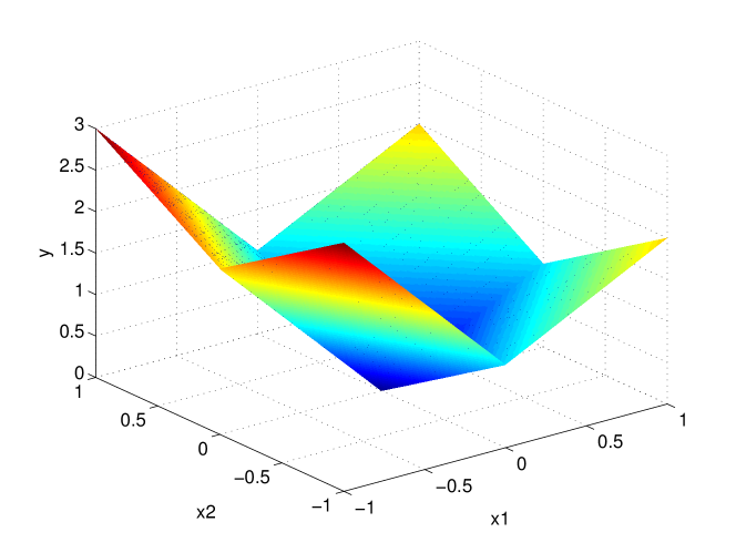
Figure 3: The 3-D plot of Example 1.

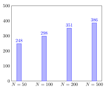
Figure 4: The number of initial points that lead to the smallest objective values.

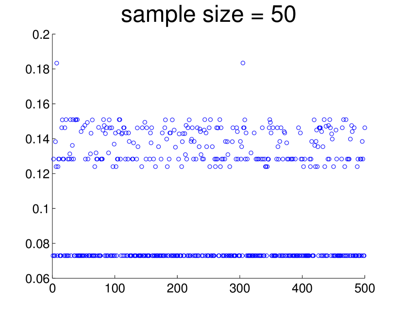
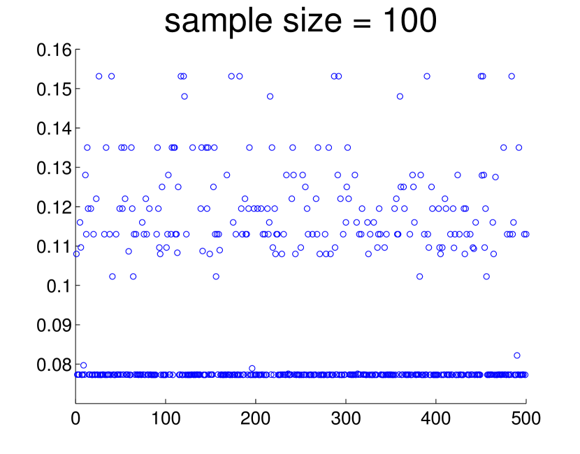
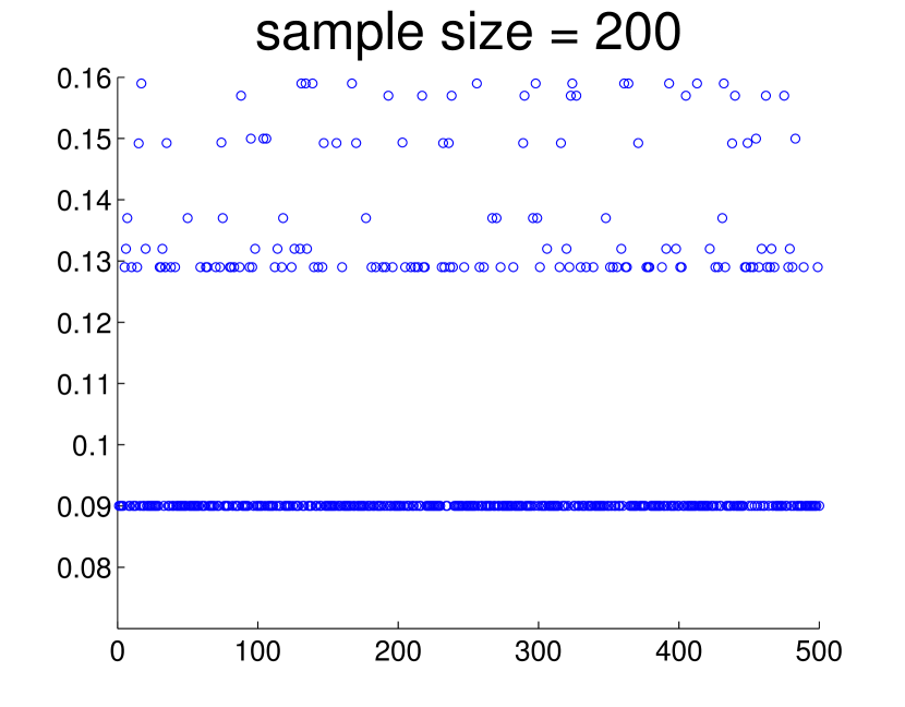
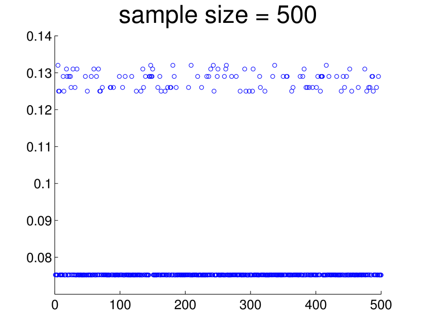
Figure 5: The objective values computed by the MM+SN algorithm of Example 1.

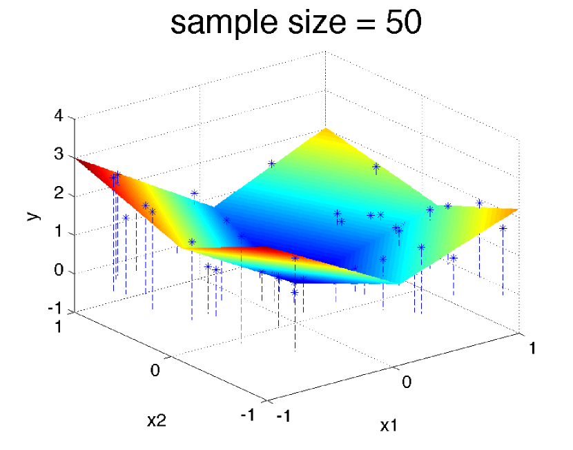
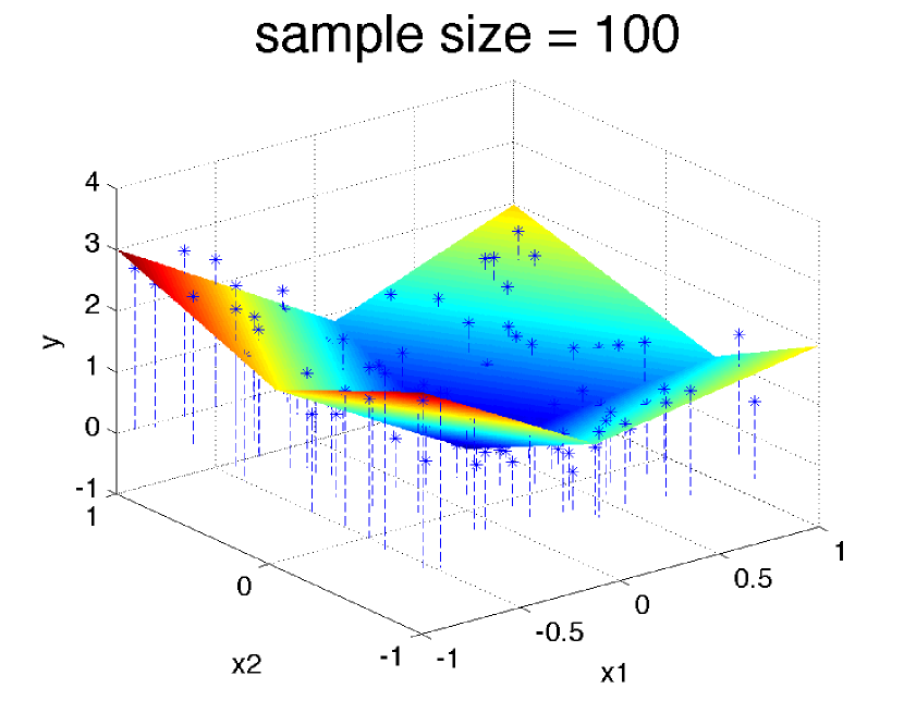
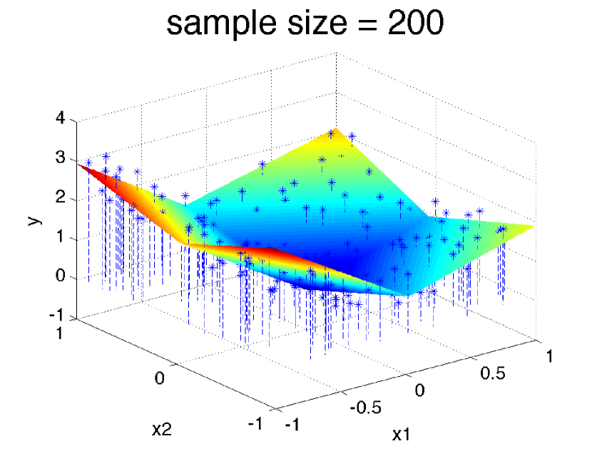
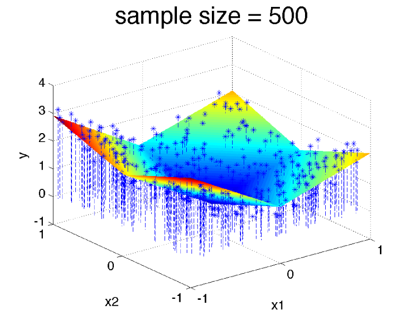
Figure 6: The solutions of Example 1 with the smallest objective values.

Example 2. Next we consider a 2-dimensional nonconvex piecewise affine model

$$y=\max\left\{x_{1}-2x_{2}\,,\,-2x_{1}+x_{2}+1\right\}-\max\left\{3x_{1}-2x_{2}\,,\,2x_{1}+5x_{2}\right\}+\varepsilon,$$

whose 3D-plot is given in Figure 9. The projection of this figure onto $y=0$ is demonstrated in Figure 9. As in Example 1, random samples of size $N=50,100,200,500$ are generated uniformly from $[-1,1]\times[-1,1]$, and $\varepsilon$ is drawn from a uniform distribution in $[-0.5,\,0.5]$. The objective values of the computed solutions over $500$ runs are shown in Figure 10. Similar observations to Example 1 can be made with regards to the concentration of the (computed) stationary values. We also plot the solutions corresponding to smallest objective values for different sample sizes in Figure 11.

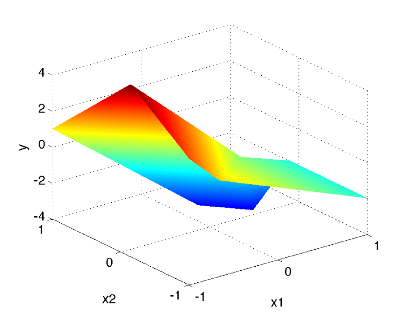
Figure 7: The 3-D plot of Example 2.

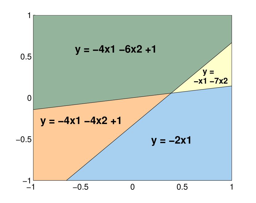
Figure 8: The projection of Example 2 onto $y=0$.

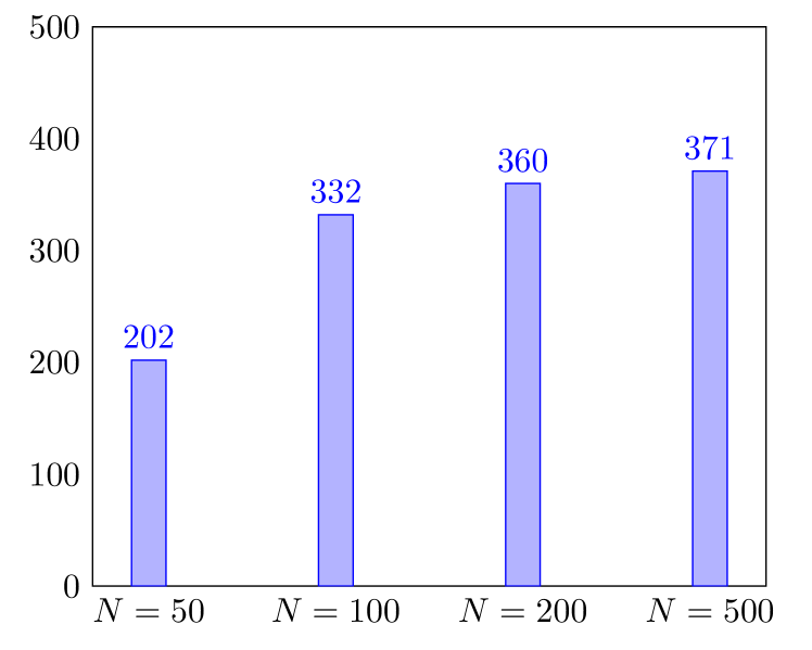
Figure 9: The number of initial points that lead to the samllest objective values.

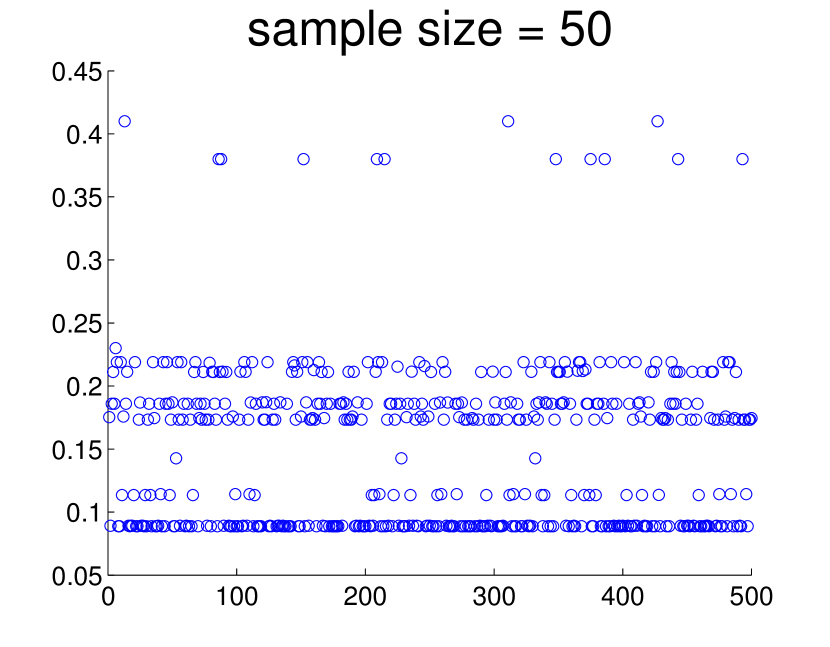
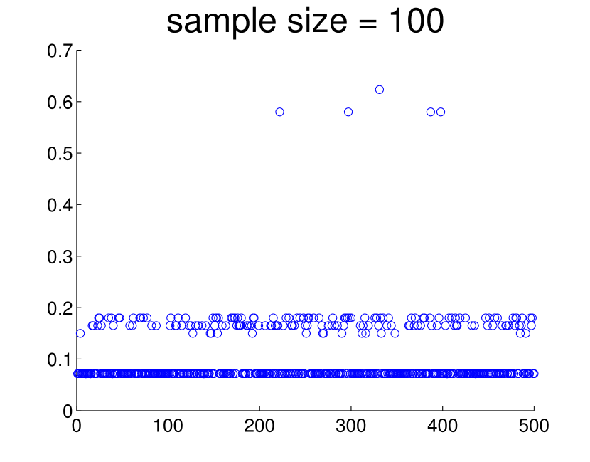
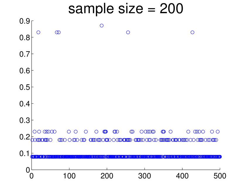
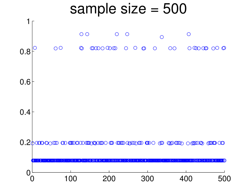
Figure 10: The objective values computed by the MM+SN algorithm of Example 2.

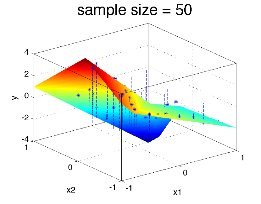
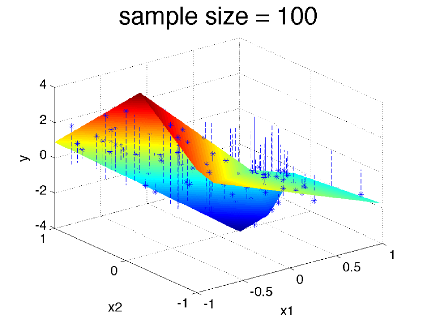
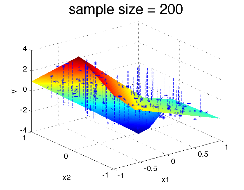
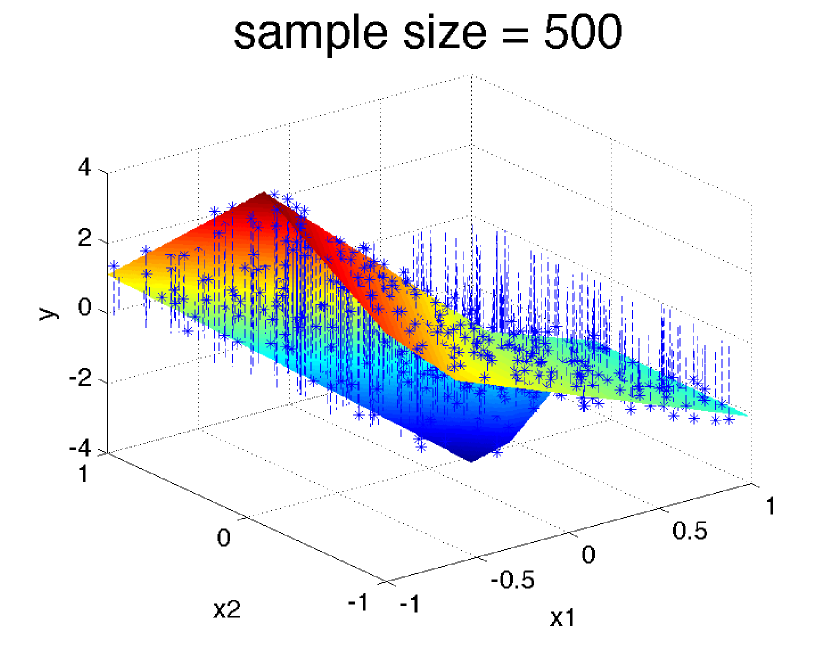
Figure 11: The solutions of Example 2 with the smallest objective values.

6.2 Real data

We also conduct the experimental evaluation of the proposed algorithm on the real datasets obtained from the UCI Repository of machine learning databases https://archive.ics.uci.edu/ml/index.php. We first list the problem characteristics and report the performance of the MM+SN method averaged over the pairs $(k_{1},k_{2})$ employed in the experiments, i.e., satisfying $1\leq k_{1},k_{2}\leq 4$ in Table 1, where the two columns under “iterations” present, respectively, the number of iterations of the MM algorithm and the total numbers of iterations of the SN algorithm. For the first four problems where the sample sizes $N$ are much larger than the dimensions $d$, no sparse regularization term is added to the model. For the other two problems where $d$ is relatively large, we take the SCAD function as the sparsity inducing penalty function. The sparse penalty parameter is estimated by 5-fold cross-validation. One can see the efficiency of the proposed MM+SN method, where it usually takes no more than $10$ SN iterations for each MM subproblem. As an illustration, Figures 13 and 13 exhibit the performance of the MM algorithm (objective values vs iteration number) and the SN algorithm ($\log_{10}\|\nabla\xi(\lambda^{k},\mu^{k};\widehat{z}^{\,\nu})\|$ vs iteration number) for solving the “auto MPG” problem with $(k_{1},k_{2})=(2,2)$.

problem name	$N$	$d$	iterations		time
			MM	SN
banknote authentication	1372	4	9	72	3.5 s
concrete compressive strength	1030	8	23	197	10.8 s
auto MPG	392	7	25	185	3.9 s
airfoil self-noise	1503	5	18	156	12.3 s
Libras Movement	360	91	22	187	14.7 s
Communities and Crime	2215	147	31	251	43.7 s

Table 1: The performance of the MM+SN algorithm

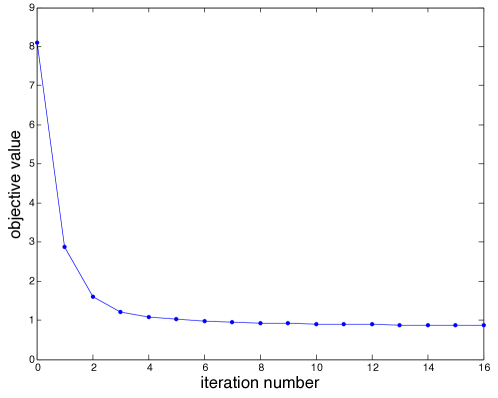
Figure 12: The performance of the MM algorithm.

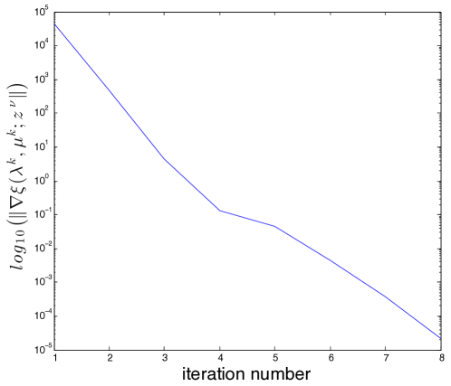
Figure 13: The performance of the SN algorithm.

To demonstrate the advantage of using the piecewise affine model over the classical linear regression model, we compare the solution of the least-squares piecewise affine regression $\theta^{\,\rm PA}$ with the ordinary least-squares solution $\theta^{\,\rm LS}\in\displaystyle\operatornamewithlimits{\mbox{argmin}}_{\theta}\displaystyle\frac{1}{2N}\sum_{s=1}^{N}\|\,y^{s}-(x^{s},1)^{T}\theta\,\|^{2}$ in the following way. Let the full dataset of each instance obtained from the UCI Repository be $T$, which is further divided into a training set $T^{\,\rm f}_{\rm training}$ and a test set $T^{\,\rm f}_{\rm test}$ for $f=1,\ldots,5$ by 5-fold cross-validation. For each fold, we find the estimator $\theta^{\,{\rm PA},\rm f}$ based on the training set $T^{\,\rm f}_{\rm training}$ by choosing the solution with the smallest objective value over $20$ runs of the MM+SN algorithm (with each run corresponding to one initial point). Such a $\theta^{\,\rm PA,f}$ is likely to be an (un-proven) global minimizer of the nonconvex least-squares piecewise affine regression program. We compute the prediction errors of the two estimators respectively by

$${\rm E}_{{\rm PA}}\triangleq\displaystyle\sum_{\rm f=1}^{5}\frac{1}{|T^{\rm f}_{\rm test}|}\sum_{s\in T_{\rm test}^{\rm f}}\left(y_{s}-\psi(x^{s};\theta^{\rm PA,f})\right)^{2},{\rm E}_{{\rm LS}}\triangleq\displaystyle\sum_{\rm f=1}^{5}\frac{1}{|T^{\rm f}_{\rm test}|}\sum_{s\in T^{\rm f}_{\rm test}}\left(y_{s}-(x^{s},1)^{T}\theta^{\,{\rm LS,f}}\right)^{2}.$$

We take $100$ simulations and report the average ratio ${\rm E}_{\rm PA}/{\rm E}_{\rm LS}$ for different choices of $(k_{1},k_{2})$ in Table 2. It can be seen that all piecewise affine results are better than the linear regression results ($k_{1}=k_{2}=1$); moreover, with proper choices of $(k_{1},k_{2})$, the prediction error given by the piecewise affine regression model is significantly smaller than that given by the linear regression model as highlighted by the best entry in each table.

As a final remark, we have observed in our simulation studies that even when the true model is linear, the continuous piecewise affine regression fits (for different choices of $k_{1}$ and $k_{2}$) are very close to that of linear regression, i.e., the ratios of the prediction errors (in 5-fold cross validation as given in Table 2) are all very close to 1. This provides further evidence that the continuous piecewise affine regression model could be a worthwhile and useful extension of linear regression.

banknote authentication						concrete compressive strength
	$1$	$2$	$3$	$4$			$1$	$2$	$3$	$4$
$1$	$1.00$	$0.74$	$0.68$	$0.67$		$1$	$1.00$	$0.74$	$0.47$	$0.38$
$2$	$0.84$	$0.73$	$0.65$	$0.63$		$2$	$0.85$	$0.46$	$0.39$	$0.39$
$3$	$0.81$	$0.72$	$0.74$	$0.74$		$3$	$0.82$	$0.65$	$0.62$	$0.61$
$4$	$0.85$	$0.71$	$0.69$	$0.74$		$4$	$0.77$	$0.54$	$0.57$	$0.60$
auto MPG						airfoil self-noise
	$1$	$2$	$3$	$4$			$1$	$2$	$3$	$4$
$1$	$1.00$	$0.77$	$0.72$	$0.77$		$1$	$1.00$	$0.83$	$0.77$	$0.74$
$2$	$0.97$	$0.74$	$0.79$	$0.73$		$2$	$0.76$	$0.72$	$0.72$	$0.59$
$3$	$0.83$	$0.78$	$0.76$	$0.76$		$3$	$0.68$	$0.68$	$0.67$	$0.57$
$4$	$0.85$	$0.84$	$0.73$	$0.73$		$4$	$0.62$	$0.62$	$0.62$	$0.425$
Libras Movement						Communities and Crime
	$1$	$2$	$3$	$4$			$1$	$2$	$3$	$4$
$1$	$1.00$	$0.93$	$0.82$	$0.80$		$1$	$1.00$	$0.88$	$0.85$	$0.83$
$2$	$0.83$	$0.86$	$0.77$	$0.77$		$2$	$0.862$	$0.82$	$0.84$	$0.84$
$3$	$0.78$	$0.72$	$0.72$	$0.76$		$3$	$0.82$	$0.83$	$0.83$	$0.83$
$4$	$0.90$	$0.73$	$0.78$	$0.80$		$4$	$0.87$	$0.84$	$0.86$	$0.87$

Table 2: Ratio of the prediction error for different choices of $(k_{1},k_{2})$.

In conclusion, we have demonstrated the practical worthiness of the LS piecewise affine regression model formulated as a nonconvex nondifferentiable program and solved by the nonmonotone MM+SN method. Further applications of this method to other statistical estimation problems will be reported separately.

References

• [1] M. Ahn, J.S. Pang, and J. Xin, Difference-of-convex learning: directional stationarity, optimality, and sparsity, SIAM J. Optim., 27 (2017), pp. 1637–1665.
• [2] H. Attouch and J. Bolte, On the convergence of the proximal algorithm for nonsmooth functions involving analytic features, Math. Program., 116 (2009), pp. 5–16.
• [3] H. Attouch, J. Bolte, and B.F. Svaiter, Convergence of descent methods for semi-algebraic and tame problems: proximal algorithms, forward-backward splitting, and regularized Gauss-Seidel methods, Math. Program., 137 (2013), pp. 91–129.
• [4] A.M. Bagirov, C. Clausen, and M. Kohler, An algorithm for the estimation of a regression function by continuous piecewise linear functions, Comput. Optim. Appl., 45 (2010), pp. 159–179.
• [5] H.H. Bauschke and P.L. Combettes, Convex Analysis and Monotone Operator Theory in Hilbert Spaces, Vol. 408., Springer, New York, 2011.
• [6] D.P. Bertsekas, Nonlinear Programming, Third Edition, Athena Scientific, Belmont, Massachusetts, 2016.
• [7] P.J. Bickel and K. Doksum, Mathematical Statistics, Basic Ideas and Selected Topics, Volume I, Prentice Hall, New Jersey, 2006.
• [8] J. Bolte, A. Daniilidis A, and A. Lewis, The Łojasiewicz inequality for nonsmooth subanalytic functions with applications to subgradient dynamical systems, SIAM J. Optim., 17 (2006), pp. 1205–1223.
• [9] J. Bolte and E. Pauwels, Majorization-minimization procedures and convergence of SQP methods for semi-algebraic and tame programs, Math. Oper. Res., 41 (2016), pp. 442–465.
• [10] J. Bolte, S. Sabach, and M. Teboulle, Proximal alternating linearized minimization for nonconvex and nonsmooth problems, Math. Program., 146 (2014), pp. 459–494.
• [11] L.D. Brown, Fundamentals of Statistical Exponential Families, IMS Lecture Notes and Monographs Series, California, 1986.
• [12] E.J. Candès, M. Wakin, and S. Boyd, Enhancing sparsity by reweighted $\ell_{1}$ minimization, J. Fourier Anal. Appl., 14 (2008), pp. 877–905.
• [13] F.H. Clarke, Optimization and Nonsmooth Analysis, SIAM, 1990.
• [14] C. Cortes and V. Vapnik, Support-vector networks, Mach. Learn., 20 (1995), pp. 273-297.
• [15] Y. Cui and J.S. Pang, On the finite number of directional stationary values of piecewise programs, arXiv:1803.00190, 2018.
• [16] Y. Cui, T.H. Chang, M. Hong, and J.S. Pang, A study of piecewise linear-quadratic programs, arXiv:1709.05758, 2018.
• [17] A.P. Dempster, N.M. Laird, and D.B. Rubin, Maximum likelihood from incomplete data via the EM algorithm, J. Roy. Stat. Soc. B: Met., 39 (1977), pp. 1–38.
• [18] H. Dong, M. Ahn, and J.S. Pang, Structural properties of affine sparsity constraints, Math. Program., in print, 2018.
• [19] D. Dunson and L.A. Hannah, Bayesian non-parametric multivariate convex regression, arXiv:1109.0322, 2011.
• [20] D. Dunson and L.A. Hannah, Multivariate convex regression with adaptive partitioning, J. Mach. Learn. Res., 14 (2013), pp. 3261–3294.
• [21] F. Facchinei and J.S. Pang, Finite-dimensional Variational Inequalities and Complementarity Problems, Springer, New York, 2003.
• [22] J. Fan and R. Li, Variable selection via nonconcave penalized likelihood and its oracle properties, J. Am. Stat. Assoc., 96 (2001), pp. 1348–1360.
• [23] X. Glorot, A. Bordes, and Y. Bengio, Deep sparse rectifier neural networks, In Proceedings of the 14th International Conference on Artificial Intelligence and Statistics, 2011, pp. 315–323.
• [24] G. Hahn, M. Banergjee, and B. Sen, Parameter estimation and inference in a continuous piecewise linear regression model, Technical report, Columbia University, 2016.
• [25] P. Hartman, On functions representable as a difference of convex functions, Pac. J. Optim., 9 (1959), pp. 707–713.
• [26] T. Hastie, R. Tibshirani, and M. Weinwright, Statistical Learning with Sparsity: The Lasso and Generalizations, CRC Press, 2015.
• [27] D.R. Hunter and K. Lange, A tutorial on MM algorithms, Am. Stat., 58 (2004), pp. 30–37.
• [28] R. Koenker and Jr G. Bassett, Regression quantiles, Econometrica, 46 (1978), pp. 33–50.
• [29] M. Kojima and S. Shindo, Extensions of Newton and quasi-Newton methods to systems of PC1 Equations, J. Oper. Res. Soc. Jpn., 29 (1986), pp. 352–374.
• [30] B. Kummer, Newton’s method for nondifferentiable functions, In Advances in Mathematical Optimization, Akademie-Verlag, Berlin, 1988, pp. 114–125.
• [31] K. Lange, MM Optimization Algorithms, SIAM, 2016.
• [32] H.A. Le Thi, V.N. and D.T. Pham, Convergence analysis of difference-of-convex algorithm with subanalytic data, J. Optim. Theory Appl., 179 (2018), pp. 103–126.
• [33] H.A. Le Thi and D.T. Pham, The DC programming and DCA revised with DC models of real world nonconvex optimization problems, Ann. Oper. Res., 133 (2005), pp. 25–46.
• [34] H.A. Le Thi, D.T. Pham, and X.T. Vo, DC approximation approaches for sparse optimization, Eur. J. Oper. Res., 244 (2015), pp. 26–46.
• [35] X. Li, D.F. Sun, and K.C. Toh, A highly efficient semismooth Newton augmented Lagrangian method for solving Lasso problems, SIAM J. Optim., 28 (2018), pp. 433–458.
• [36] Z. Lu, Z. Zhou, and Z. Sun, Enhanced proximal DC algorithms with extrapolation for a class of structured nonsmooth DC minimization, Math. Program., in print, 2018.
• [37] J. Mairal, Optimization with first-order surrogate functions, In Proceedings of the 30th International Conference on Machine Learning, 2013, pp. 783–791.
• [38] J. Mairal, Incremental majorization-minimization optimization with application to large-scale machine learning, SIAM J. Optim., 25 (2015), pp. 829–855.
• [39] R. Mazumder, A. Choudhury, G. Iyengar, and B. Sen, A computational framework for multivariate convex regression and its variants, J. Am. Stat. Assoc., in print, 2018.
• [40] R. Mifflin, Semismooth and semiconvex functions in constrained optimization, SIAM J. Control Optim., 15 (1977), pp. 959–972.
• [41] A. Milzarek and M. Ulbrich, A semismooth Newton method with multidimensional filter globalization for $\ell_{1}$ optimization, SIAM J. Optim., 24 (2014), pp. 298–333.
• [42] B.S. Mordukhovich, Variational Analysis and Generalized Differentiation I, Springer, 2006.
• [43] V. Nair and G.E. Hinton, Rectified linear units improve restricted Boltzmann machines, In Proceedings of the 27th International Conference on Machine Learning, 2010, pp. 807–814.
• [44] J. M. Ortega and W. C. Rheinboldt, Iterative solution of nonlinear equations in several variables, Vol. 30, SIAM, 1970.
• [45] J.S. Pang, Newton’s method for B-differentiable equations, Math. Oper. Res., 15 (1990), pp. 311–341.
• [46] J.S. Pang and L. Qi, A globally convergent Newton method for convex SC1 minimization problems, J. Optim. Theory Appl., 85 (1995), pp. 633–648.
• [47] J.S. Pang, M. Razaviyayn, and A. Alvarado, Computing B-stationary points of nonsmooth DC programs, Math. Oper. Res., 42 (2016), pp. 95–118.
• [48] D.T. Pham and H.A. Le Thi, Convex analysis approach to DC programming: Theory, algorithm and applications, Acta Mathematica Vietnamica, 22 (1997), pp. 289–355.
• [49] H. Qi and D.F. Sun, A quadratically convergent Newton method for computing the nearest correlation matrix, SIAM J. Matrix Anal. A., 28 (2006), pp. 360–385.
• [50] L. Qi and J. Sun, A nonsmooth version of Newton’s method, Math. Program., 58 (1993), pp. 353–367.
• [51] R.T. Rockafellar, Convex Analysis, Princeton University Press, Princeton, 1970.
• [52] R.T. Rockafellar and R.J.-B. Wets, Variational Analysis, Springer, New York, 1998.
• [53] S. Scholtes, Introduction to Piecewise Differentiable Equations, Springer Briefs in Optimization, 2002.
• [54] J. Sun, On Monotropic Piecewise Quadratic Programming, Ph.D. dissertation, Department of Applied Mathematics, University of Washington, 1986.
• [55] J. Sun, On the structure of convex piecewise quadratic functions, J. Optim. Theory Appl., 72 (1992), pp. 499–510.
• [56] R. Tibshirani, M. Saunders, S. Rosset, J. Zhu, and K. Knight, Sparsity and smoothness via the fused lasso, J. Roy. Stat. Soc. B: Met., 67 (2005), pp. 91–108.
• [57] B. Wen, X. Chen, and T.K. Pong, A proximal difference-of-convex algorithm with extrapolation, Comput. Optim. Appl., 2 (2018), pp. 297–324.
• [58] C.J. Wu, On the convergence properties of the EM algorithm, Ann. Stat., 11 (1983), pp. 95–103.
• [59] L.Q. Yang, D.F. Sun, and K.C. Toh, SDPNAL+: a majorized semismooth Newton-CG augmented Lagrangian method for semidefinite programming with nonnegative constraints, Math. Program. Comput., 7 (2015), pp. 331–366.
• [60] P. Yin, Y. Lou, Q. He and J. Xin, Minimization of $\ell_{1}-\ell_{2}$ for compressed sensing, SIAM J. Sci. Comput., 37 (2015), pp. 536–563.
• [61] D. Yu and L. Deng, Automatic Speech Recognition: A Deep Learning Approach, Signals and Communications Technology, Springer, 2015.
• [62] M. Yuan and Y. Lin, Model selection and estimation in regression with grouped variables, J. Roy. Stat. Soc. B: Met., 68 (2006), pp. 49–67.
• [63] C. Zhang, Nearly unbiased variable selection under minimax concave penalty, Ann. Stat., 38 (2010), pp. 894–942.
• [64] C. Zhang, M. Pham, S. Fu, and Y. Liu, Robust multicategory support vector machines using difference convex algorithm, Math. Program., 169 (2018), pp. 277–305.
• [65] X. Zhao, D.F. Sun, and K.C. Toh, A Newton-CG augmented Lagrangian method for semidefinite programming, SIAM J. Optim., 20 (2010), pp. 1737–1765.