Breaking the habit — the peculiar 2016 eruption of
the unique recurrent nova M31N 2008-12a.

Abstract

Since its discovery in 2008, the Andromeda galaxy nova M31N 2008-12a has been observed in eruption every single year. This unprecedented frequency indicates an extreme object, with a massive white dwarf and a high accretion rate, which is the most promising candidate for the single-degenerate progenitor of a type-Ia supernova known to date. The previous three eruptions of M31N 2008-12a have displayed remarkably homogeneous multi-wavelength properties: (i) From a faint peak, the optical light curve declined rapidly by two magnitudes in less than two days; (ii) Early spectra showed initial high velocities that slowed down significantly within days and displayed clear He/N lines throughout; (iii) The supersoft X-ray source (SSS) phase of the nova began extremely early, six days after eruption, and only lasted for about two weeks. In contrast, the peculiar 2016 eruption was clearly different. Here we report (i) the considerable delay in the 2016 eruption date, (ii) the significantly shorter SSS phase, and (iii) the brighter optical peak magnitude (with a hitherto unobserved cusp shape). Early theoretical models suggest that these three different effects can be consistently understood as caused by a lower quiescence mass-accretion rate. The corresponding higher ignition mass caused a brighter peak in the free-free emission model. The less-massive accretion disk experienced greater disruption, consequently delaying re-establishment of effective accretion. Without the early refueling, the SSS phase was shortened. Observing the next few eruptions will determine whether the properties of the 2016 outburst make it a genuine outlier in the evolution of M31N 2008-12a.

1 Introduction

Recurrent novae with frequent eruptions are new and exciting objects at the interface between the parameter spaces of novae and type Ia supernovae (SNe Ia). Novae are periodic thermonuclear eruptions on the surfaces of white dwarfs (WDs) in mass-transfer binaries (see Bode & Evans, 2008; José, 2016; Starrfield et al., 2016, for comprehensive reviews on nova physics). In SNe Ia, a carbon-oxygen (CO) WD approaches the Chandrasekhar (1931) mass limit to be destroyed in a thermonuclear explosion. Theoretical models show that a CO WD can indeed grow from a low initial mass through many nova cycles to eventually become a SN Ia (e.g., Yaron et al., 2005; Newsham et al., 2014; Hillman et al., 2016).

Only for massive WDs with high accretion rates do the periods of the nova cycles become shorter than $\sim 100$ yr (Starrfield et al., 1985; Yaron et al., 2005; Hernanz & José, 2008; Kato et al., 2014) — the (current) empirical limit to observe a nova erupting more than once. These are called recurrent novae (RNe) and have been observed in the Galaxy and its closest neighbors (see, for example, Shore et al., 1991; Schaefer, 2010; Shafter et al., 2015; Bode et al., 2016). The extreme physics necessary to power the high eruption frequency of the RNe with the shortest periods makes them the most promising (single-degenerate) SN Ia progenitor candidates known today (Kato et al., 2015).

Among the ten RNe in the Galaxy, U Scorpii has the shortest period with inter-eruption durations as short as eight years (Schaefer, 2010). Another nova with rapid eruptions has recently been found in the Large Magellanic Cloud (LMCN 1968-12a with 5 yr; Mroz & Udalski, 2016; Darnley et al., 2016a; Kuin et al., 2018). However, it is the nearby Andromeda galaxy (M 31) which hosts six RNe with eruption periods of less than 10 yr. Due to its proximity and relatively high stellar mass (within the Local Group), M 31 has been a target of optical nova surveys for a century. Starting with the first discovery by Ritchey (1917), exactly 100 yr ago, and the first monitoring survey by Hubble (1929), the community has gradually built a rich database of more than 1000 nova candidates in M 31 (see Pietsch et al., 2007; Pietsch, 2010, and their on-line database). Crucially, the low foreground extinction toward M 31 ($N_{\rm H}$ = 0.7$\times 10^{21}$ cm^-2, Stark et al., 1992) favours X-ray monitoring surveys for novae (Pietsch et al., 2007; Henze et al., 2010, 2011, 2014b).

The unparalleled M 31 nova sample contains 18 known RNe (Shafter et al., 2015; Hornoch & Shafter, 2015; Sin et al., 2017). Among them there are five RNe with recurrence periods between four and nine years. Those objects are: M31N 1990-10a (9 yr period; Henze et al., 2016f, e; Ederoclite et al., 2016; Fabrika et al., 2016), M31N 2007-11f (9 yr period; Sin et al., 2017; Fabrika et al., 2017), M31N 1984-07a (8 yr period Hornoch & Vrastil, 2012; Shafter et al., 2015), M31N 1963-09c (5 yr period Rosino, 1973; Henze et al., 2014b; Williams et al., 2015b, a; Henze et al., 2015c, b), and M31N 1997-11k (4 yr period Henze et al., 2009; Shafter et al., 2015).

The indisputable champion of all RNe, however, is M31N 2008-12a. Since its discovery in 2008 (by Nishiyama & Kabashima, 2008), this remarkable nova has been seen in eruption every single year (Darnley et al., 2016d, hereafter DHB16, see Table 1). Beginning in 2013, our group has been studying the eruptions of M31N 2008-12a with detailed multi-wavelength observations. For the 2013 eruption we found a fast optical evolution (Darnley et al., 2014, hereafter DWB14) and a supersoft X-ray source (SSS; Krautter, 2008) phase of only two weeks (Henze et al. 2014a, hereafter HND14, also see Tang et al. 2014). The SSS stage, powered by nuclear burning within the hydrogen-rich envelope remaining on the WD after the eruption, typically lasts years to decades in regular novae (Schwarz et al., 2011; Henze et al., 2014b; Osborne, 2015). The SSS phase of the 2014 eruption was similarly short (Henze et al., 2015d, hereafter HND15) and we collected high-cadence, multi-color optical photometry (Darnley et al., 2015c, hereafter DHS15). In Henze et al. (2015a, hereafter HDK15) we predicted the date of the 2015 eruption with an accuracy of better than a month and followed it with a large multi-wavelength fleet of telescopes (DHB16).

Table 1: All Known Eruption Dates of M31N 2008-12a.

Eruption date	SSS-on date	Days since	Detection wavelength	References
(UT)	(UT)	last eruption	(observatory)
(1992 Jan 28)	1992 Feb 03	$\cdots$	X-ray (ROSAT)	1, 2
(1993 Jan 03)	1993 Jan 09	341	X-ray (ROSAT)	1, 2
(2001 Aug 27)	2001 Sep 02	$\cdots$	X-ray (Chandra)	2, 3
2008 Dec 25	$\cdots$	$\cdots$	Visible (Miyaki-Argenteus)	4
2009 Dec 02	$\cdots$	342	Visible (PTF)	5
2010 Nov 19	$\cdots$	352	Visible (Miyaki-Argenteus)	2
2011 Oct 22.5	$\cdots$	337.5	Visible (ISON-NM)	5–8
2012 Oct 18.7	$<2012$ Nov 06.45	362.2	Visible (Miyaki-Argenteus)	8–11
2013 Nov $26.95\pm 0.25$	$\leq 2013$ Dec 03.03	403.5	Visible (iPTF); UV/X-ray (Swift)	5, 8, 11–14
2014 Oct $02.69\pm 0.21$	2014 Oct $08.6\pm 0.5$	$309.8\pm 0.7$	Visible (LT); UV/X-ray (Swift)	8, 15
2015 Aug $28.28\pm 0.12$	2015 Sep $02.9\pm 0.7$	$329.6\pm 0.3$	Visible (LCO); UV/X-ray (Swift)	14, 16–18
2016 Dec $12.32\pm 0.17$	2016 Dec $17.2\pm 1.1$	$471.7\pm 0.2$	Visible (Itagaki); UV/X-ray (Swift)	19–23

The overall picture of M31N 2008-12a that had been emerging through the recent campaigns indicated very regular properties (see DHB16 for a detailed description): Successive eruptions occurred every year with a predictable observed period of almost one year ($347\pm 10$ d). The optical light curve rose within about a day to a maximum below 18th mag (faint for an M 31 nova) and then immediately declined rapidly by 2 mag in about 2 d throughout the UV/optical bands. The SSS counterpart brightened at around day 6 after eruption and disappeared again into obscurity around day 19 ($t_{\mbox{\small{on}}}=5.6\pm 0.7$ d and $t_{\mbox{\small{off}}}=18.6\pm 0.7$ d in 2015). Even the time evolution of the SSS effective temperatures in 2013–2015, albeit derived from low-count Swift spectra, closely resembled each other.

Far UV spectroscopy of the 2015 eruption uncovered no evidence for neon in the ejecta (Darnley et al., 2017c, hereafter DHG17S). Therefore, these observations could not constrain the composition of the WD, since an ONe core might be shielded by a layer of He that grows with each eruption and H-burning episode. Modeling of the accretion disk, based on late-time and quiescent Hubble Space Telescope (HST) photometry, indicated that the accretion disk survives the eruptions, and that the quiescent accretion rate was both extremely variable and remarkably high $\sim 10^{-6}\,M_{\odot}\,\mathrm{yr}^{-1}$ (Darnley et al., 2017b, hereafter DHG17P). Theoretical simulations found the eruption properties to be consistent with an $1.38\,M_{\sun}$ WD accreting at a rate of $1.6\times 10^{-7}\,M_{\sun}$ yr^-1 (Kato et al., 2015, 2016, 2017). DHG17P also produced the first constraints on the mass donor a, possibly irradiated, red-clump star with $L_{\mathrm{donor}}=103^{+12}_{-11}\,L_{\odot}$, $R_{\mathrm{donor}}=14.14^{+0.46}_{-0.47}\,R_{\odot}$, and $T_{\mathrm{eff,donor}}=4890\pm 110$ K. Finally, DHG17P utilized these updated system parameters to refine the time remaining for the WD to grow to the Chandrasekhar mass to be $<20$ kyr.

By all accounts, M31N 2008-12a appeared to have become remarkably predictable even for a RN (see also Darnley, 2017, for a recent review). Then everything changed. The 2016 eruption, predicted for mid September, did not occur until December 12th (Itagaki et al., 2016); leading to a frankly suspenseful monitoring campaign. Once detected, the optical light curve was observed to peak at a significantly brighter level than previously seen (Erdman et al., 2016; Burke et al., 2016), before settling into the familiar rapid decline. When the SSS duly appeared around day 6 (Henze et al., 2016c) we believed the surprises were over. We were wrong (Henze et al., 2016d). This paper studies the unexpected behavior of the 2016 eruption of M31N 2008-12a and discusses its impact on past and future observations.

2 Observations and data analysis of the 2016 Eruption

In this section, we describe the multi-wavelength set of telescopes used in studying the 2016 eruption together with the corresponding analysis procedures. All errors are quoted to $1\sigma$ and all upper limits to $3\sigma$, unless specifically stated otherwise. The majority of the statistical analysis was carried out within the R software environment (R Development Core Team, 2011). Throughout, all photometry through Johnson–Cousins filters, and the HST, XMM-Newton, and Swift flight filters are computed in the Vega system, all photometry through Sloan filters are quoted in AB magnitudes. We assume an eruption date of 2016-12-12.32 UT; discussed in detail in Sect. 3.1 and 5.1.

2.1 Visible Photometry

Like the 2014 and 2015 eruptions before it (DHS15, DHB16), the 2016 eruption of M31N 2008-12a was observed by a large number of ground-based telescopes operating in the visible regime. Unfortunately, due to poor weather conditions at many of the planned facilities, observations of the 2016 eruption are much sparser than in recent years.

A major achievement for the 2016 eruption campaign was the addition of extensive observations from the American Association of Variable Star Observers (AAVSO), along with the continued support of the Variable Star Observers League in Japan (VSOLJ; see Section 3.1 and Appendix A). Observations were also obtained from the Mount Laguna Observatory (MLO) 1.0 m telescope in California, the Ondřejov Observatory 0.65 m telescope in the Czech Republic, the Danish 1.54 m telescope at La Silla in Chile, the fully-robotic 2 m Liverpool Telescope (LT; Steele et al., 2004) in La Palma, the 2.54 m Isaac Newton Telescope (INT) at La Palma, the Palomar 48^′′ telescope in California, the 0.6 m and 1 m telescopes operated by members of the Embry Riddle Aeronautical University (ERAU) in Florida, the $2\times 8.4$ m (11.8 m eq.) Large Binocular Telescope (LBT) on Mount Graham, Arizona, the 2 m Himalayan Chandra Telescope (HCT) located at Indian Astronomical Observatory (IAO), Hanle, India, and the 2.4 m Hubble Space Telescope.

2.1.1 Hubble Space Telescope photometry

The 2016 eruption, and pre-eruption interval, of M31N 2008-12a were observed serendipitously by HST as part of Program ID: 14651. The aim of this program was to observe the proposed “Super-Remnant” surrounding M31N 2008-12a (see DHS15 and Darnley et al., 2017a). Five pairs of orbits were tasked to obtain narrow band F657N (H$\alpha$+[N ii]) and F645N (continuum) observations using Wide Field Camera 3 (WFC3) in the UVIS mode. Each orbit utilized a three-point dither to enable removal of detector defects. A ‘post-flash’ of 12 electrons was included to minimize charge transfer efficiency (CTE) losses.

The WFC3/UVIS observations were reduced using the STScI calwf3 pipeline (v3.4; Dressel, 2012), which includes CTE correction. Photometry of M31N 2008-12a was subsequently performed using DOLPHOT (v2.0; Dolphin, 2000) employing the standard WFC3/UVIS parameters as quoted in the accompanying manual. The resultant photometry is reported in Table 2, a full description of these HST data and their analysis will be reported in a follow-up paper.

Table 2: Hubble Space Telescope Photometry of the 2016 Eruption of M31N 2008-12a.

Date	$\Delta t$	MJD 57,000+		Exposure	Filter	S/N	Photometry
(UT)	(days)	Start	End	time (s)
2016-12-08.014	-4.306	729.971	730.058	$3\times 898$	F657N	19.7	$23.143\pm 0.055$
2016-12-09.312	-3.008	731.295	731.329	$3\times 898$	F657N	14.5	$23.500\pm 0.075$
2016-12-10.305	-2.015	732.288	732.322	$3\times 898$	F657N	16.8	$23.421\pm 0.065$
2016-12-11.060	-1.260	733.016	733.104	$3\times 898$	F657N	17.8	$23.327\pm 0.061$
2016-12-17.081	+4.761	739.043	739.118	$3\times 898$	F657N	165.3	$19.348\pm 0.007$
2016-12-08.140	-4.180	730.102	730.179	$3\times 935$	F645N	13.4	$23.591\pm 0.081$
2016-12-09.378	-2.942	731.360	731.396	$3\times 935$	F645N	11.3	$23.806\pm 0.096$
2016-12-10.371	-1.949	732.353	732.389	$3\times 935$	F645N	12.5	$23.589\pm 0.087$
2016-12-11.186	-1.134	733.148	733.225	$3\times 935$	F645N	15.5	$23.413\pm 0.070$
2016-12-17.159	+4.839	739.120	739.197	$3\times 935$	F645N	85.0	$20.488\pm 0.013$

2.1.2 Ground-Based Photometry

Data from each contributing telescope were reduced following the standard procedures for those facilities, full details for those previously employed in observations of M31N 2008-12a are presented in the Appendix of DHB16. For all the new facilities successfully taking data in this campaign we provide detailed information in Appendix A. Photometry was also carried out in a similar manner to that reported in DHB16, using the identified secondary standards as presented in DHB16 (see their Table 10).

Preliminary photometry from several instruments was first published by the following authors as the optical light curve was evolving: Itagaki et al. (2016), Erdman et al. (2016), Burke et al. (2016), Shafter et al. (2016), Darnley & Hounsell (2016), Kaur et al. (2016), Hornoch et al. (2016), Tan et al. (2016), Naito et al. (2016), Darnley et al. (2016c), and Darnley (2016). All photometry from the 2016 eruption of M31N 2008-12a is provided in Table B.

2.2 Visible Spectroscopy

The spectroscopic confirmation of the 2016 eruption of M31N 2008-12a was announced by Darnley et al. (2016b), with additional spectroscopic follow-up reported in Pavana & Anupama (2016). A summary of all optical spectra of the 2016 eruption of M31N 2008-12a is shown in Table 3, all the spectra are reproduced in Figure 16.

We obtained several spectra of the 2016 eruption with SPRAT (Piascik et al., 2014), the low-resolution, high-throughput spectrograph on the LT. SPRAT covers the wavelength range of $4000-8000$ Å and uses a $1^{\prime\prime}\!\!.8$ slit, giving a resolution of $\sim$18 Å. We obtained our spectra using the blue-optimized mode. The data were reduced using a combination of the LT SPRAT reduction pipeline and standard routines in IRAF (Tody, 1993). The spectra were calibrated using previous observations of the standard star G191-B2B against data from Oke (1990) obtained via ESO. Conditions on La Palma were poor during the time frame the nova was accessible with SPRAT during the 2016 eruption, so the absolute flux levels are possibly unreliable.

We obtained an early spectrum of the nova, 0.54 days after eruption, using the Andalucía Faint Object Spectrograph and Camera (ALFOSC) on the 2.5 m Nordic Optical Telescope (NOT) at the Roque de los Muchachos Observatory on La Palma. Grism #7 and a slit width of $1^{\prime\prime}\!\!.3$ yielded a spectral resolution of 8.5 Å at the centre of the useful wavelength range $4000-7070$ Å ($R\sim 650$). The 1500 s spectrum was imaged on the $2048\times 2048$ pixel CCD #14 with binning $2\times 2$. We performed the observation under poor seeing conditions ($\sim 2^{\prime\prime}\!\!.5$). We reduced the raw images using standard IRAF procedures, and then did an optical extraction of the target spectrum with starlink/pamela (Marsh, 1989). The pixel-to-wavelength solution was computed by comparison with 25 emission lines of the spectrum of a HeNe arc lamp. We used a 4th-order polynomial that provided residuals with an rms more than 10 times smaller than the spectral dispersion.

In addition, 1.87 days after eruption, we obtained a spectrum of M31N 2008-12a using the blue channel of the 10 m Hobby Eberly Telescope’s (HET) new integral-field Low Resolution Spectrograph (LRS2-B; Chonis et al., 2014, 2016). This dual-beam instrument uses 280 fibers and a lenslet array to produce spectra with a resolution of $R\sim 1910$ between the wavelengths 3700 and 4700 Å, and $R\sim 1140$ between 4600 and 7000 Å over a $12^{\prime\prime}\times 6^{\prime\prime}$ region of sky. The seeing for our observations was relatively poor ($1\farcs 8$), and the total exposure time was 30 minutes, split into 3 ten-minute exposures.

Reduction of the LRS2-B data was accomplished using Panacea, a general-purpose IFU reduction package built for HET. After performing the initial CCD reductions (overscan removal and bias subtraction), we derived the wavelength solution, trace model, and spatial profile of each fiber using data from twilight sky exposures taken at the beginning of the night. From these models, we extracted each fiber’s spectrum and rectified the wavelength to a common grid. Finally, at each wavelength in the grid, we fit a second order polynomial to the M31’s background starlight and subtracted that from the gaussian-shaped point-source assumed for the nova.

Two epochs of spectra were obtained using the Himalayan Faint Object Spectrograph and Camera (HFOSC) mounted on the 2 m Himalayan Chandra Telescope (HCT) located at Indian Astronomical Observatory (IAO), Hanle, India. HFOSC is equipped with a 2k$\times$4k E2V CCD with pixel size of $15\times 15$ $\mu$m. Spectra were obtained in the wavelength range $3800-8000$ Å on 2016 December 13.61 and 14.55 UT. The spectroscopic data were bias subtracted and flat field corrected and extracted using the optimal extraction method. An FeAr arc lamp spectrum was used for wavelength calibration. The spectrophotometric standard star Feige 34 was used to obtain the instrumental response for flux calibration.

Three spectra were obtained with the 3.5 m Astrophysical Research Consortium (ARC) telescope at the Apache Point Observatory (APO), during the first half of the night on 2016 December 12, 13, and 17 (UT December 13, 14, and 18). We observed with the Dual Imaging Spectrograph (DIS): a medium dispersion long slit spectrograph with separate collimators for the red and blue part of the spectrum and two 2048$\times$1028 E2V CCD cameras, with the transition wavelength around 5350 Å. For the blue branch, a 400 lines mm^-1 grating was used, while the red branch was equipped with a 300 lines mm^-1 grating. The nominal dispersions were 1.83 and 2.31 Å pixel^-1, respectively, with central wavelengths at 4500 and 7500 Å. The wavelength regions actually used were 3500–5400 Å and 5300–9900 Å for blue and red, respectively. A $1^{\prime\prime}\!\!.5$ slit was employed. Exposure times were 2700 s. At least three exposures were obtained per night. Each on-target series of exposures was followed by a comparison lamp exposure (HeNeAr) for wavelength calibration. A spectrum of a spectrophotometric flux standard (BD+28 4211) was also acquired during each night, along with bias and flat field calibration exposures. The spectra were reduced using Python scripts to perform standard flat field and bias corrections to the 2-D spectral images. Extraction traces and sky regions were then defined interactively on the standard star and object spectral images. Wavelength calibration was determined using lines identified on the extracted HeNeAr spectra. We then determined the solution by fitting a 3rd order polynomial to these measured wavelengths. Flux calibration was determined by measuring the ratio of the star fluxes to the known fluxes as a function of wavelength. We performed these calibrations independently for the red and blue spectra, so that the clear agreement in the overlapping regions of the wavelength ranges confirms that our calibration and reduction procedure was successful.

Table 3: Summary of the Optical Spectra of the 2016 Eruption of M31N 2008-12a.

Date (UT)	$\Delta t$	Instrument	Exposure
2017 Dec	(days)	& Telescope	time (s)
12.86	0.54$\pm$0.01	ALFOSC/NOT	$1\times 1500$
12.93	0.61$\pm$0.06	SPRAT/LT	$6\times\phantom{0}900$
13.14	0.82$\pm$0.11	DIS/ARC
13.61	1.29$\pm$0.02	HFOSC/HCT	$1\times 3600$
13.98	1.66$\pm$0.07	SPRAT/LT	$6\times\phantom{0}900$
14.12	1.80$\pm$0.08	DIS/ARC
14.19	1.87$\pm$0.02	LRS2-B/HET	$3\times\phantom{0}600$
14.55	2.23$\pm$0.02	HFOSC/HCT	$1\times 2700$
14.90	2.58$\pm$0.05	SPRAT/LT	$6\times\phantom{0}900$
15.91	3.59$\pm$0.02	SPRAT/LT	$3\times\phantom{0}900$
16.85	4.53$\pm$0.02	SPRAT/LT	$3\times\phantom{0}900$
18.15	5.83$\pm$0.05	DIS/ARC

2.3 X-ray and UV observations

A Neil Gehrels Swift Observatory (Gehrels et al., 2004) target of opportunity (ToO) request was submitted immediately after confirming the eruption and the satellite began observing the nova on 2016-12-12.65 UT (cf. Henze et al., 2016b), only four hours after the optical discovery. All Swift observations are summarized in Table 4. The Swift target ID of M31N 2008-12a  is always 32613. Because of the low-Earth orbit of the satellite, a Swift observation is normally split into several snapshots, which we list separately in Table 11.

Table 4: Swift Observations of M31N 2008-12a for the 2016 Eruption.

ObsID	Expa	Dateb	MJDb	$\Delta t^{c}$	uvw2d	XRT Ratee
	(ks)	(UT)	(d)	(d)	(mag)	($10^{-2}$ ct s-1)
00032613183	3.97	2016-12-12.65	57734.65	0.33	$16.7\pm 0.1$	$<0.3$
00032613184	4.13	2016-12-13.19	57735.19	0.87	$17.3\pm 0.1$	$<0.2$
00032613185	3.70	2016-12-14.25	57736.26	1.94	$17.9\pm 0.1$	$<0.3$
00032613186	3.23	2016-12-15.65	57737.65	3.33	$18.6\pm 0.1$	$<0.4$
00032613188	1.10	2016-12-16.38	57738.38	4.06	$18.7\pm 0.1$	$<0.7$
00032613189	3.86	2016-12-18.10	57740.10	5.78	$19.3\pm 0.1$	$0.6\pm 0.1$
00032613190	4.03	2016-12-19.49	57741.50	7.18	$20.0\pm 0.2$	$0.4\pm 0.1$
00032613191	2.02	2016-12-20.88	57742.89	8.57	$20.6\pm 0.3$	$1.9\pm 0.3$
00032613192	3.95	2016-12-21.49	57743.49	9.17	$20.9\pm 0.3$	$1.5\pm 0.2$
00032613193	2.53	2016-12-22.68	57744.69	10.37	$20.4\pm 0.2$	$1.7\pm 0.3$
00032613194	2.95	2016-12-23.67	57745.68	11.36	$20.8\pm 0.3$	$1.4\pm 0.2$
00032613195	2.90	2016-12-24.00	57746.01	11.69	$20.5\pm 0.2$	$0.7\pm 0.2$
00032613196	2.73	2016-12-25.00	57747.01	12.69	$>21.1$	$0.6\pm 0.2$
00032613197	2.71	2016-12-26.20	57748.20	13.88	$>21.1$	$0.3\pm 0.2$
00032613198	2.84	2016-12-27.72	57749.73	15.41	$>21.1$	$<0.5$
00032613199	3.23	2016-12-28.19	57750.19	15.87	$>21.2$	$<0.4$
00032613200	2.65	2016-12-29.45	57751.46	17.14	$>21.1$	$<0.5$
00032613201	3.05	2016-12-30.05	57752.05	17.73	$>20.9$	$<0.4$
00032613202	2.88	2016-12-31.58	57753.58	19.26	$>21.1$	$<0.3$

Table 5: Stacked Swift UVOT Observations and Photometry as Plotted in Figure 5.

ObsIDsa	Expb	Datec	MJDc	$\Delta t^{c}$	Lengthd	uvw2
	(ks)	(UT)	(d)	(d)	(d)	(mag)
00032613196/198	8.3	2016-12-26.37	57748.37	14.05	2.72	$21.7\pm 0.4$
00032613199/200	5.9	2016-12-28.83	57750.83	16.51	1.27	$<21.5$

In addition, we triggered a 100 ks XMM-Newton (Jansen et al., 2001) ToO that was originally aimed at obtaining a high-resolution X-ray spectrum of the SSS variability phase. Due to the inconvenient eruption date, 14 days before the XMM-Newton window opened, and the surprisingly fast light curve evolution, discussed in detail below, only low resolution spectra and light curves could be obtained. The XMM-Newton object ID is 078400. The ToO was split into two observations which are summarized in Table 6. Since 2008, no eruption of M31N 2008-12a  had occurred within one of the relatively narrow XMM-Newton visibility windows from late December to mid February and July to mid August (cf. Table 1).

The Swift UV/optical telescope (UVOT, Roming et al., 2005) magnitudes were obtained via the HEASoft (v6.18) tool uvotsource; based on aperture photometry of carefully selected source and background regions. We stacked individual images using uvotimsum. In contrast to previous years, our 2016 coverage exclusively used the uvw2 filter which has a central wavelength of 1930 Å. The photometric calibration assumes the UVOT photometric (Vega) system (Poole et al., 2008; Breeveld et al., 2011) and has not been corrected for extinction.

In the case of the Swift X-ray telescope (XRT; Burrows et al., 2005) data we used the on-line software of Evans et al. (2009) to extract count rates and upper limits for each observation and snapshot, respectively. Following the recommendation for SSSs, we extracted only grade-zero events. The on-line software uses the Bayesian formalism of Kraft et al. (1991) to estimate upper limits for low numbers of counts. All XRT observations were taken in the photon counting (PC) mode.

The XMM-Newton X-ray data were obtained with the thin filter for the pn and MOS detectors of the European Photon Imaging Camera (EPIC; Strüder et al., 2001; Turner et al., 2001). They were processed with XMM-SAS (v15.0.0) starting from the observation data files (ODF) and using the most recent current calibration files (CCF). We used evselect to extract spectral counts and light curves from source and background regions that were defined by eye on the event files from the individual detectors. We filtered the event list by extracting a background light curve in the 0.2–0.7 keV range (optimized after extracting the first spectra, see Section 4.2) and removing the episodes of flaring activity.

In addition, we obtained UV data using the XMM-Newton optical/UV monitor telescope (OM; Mason et al., 2001). All OM exposures were taken with the uvw1 filter, which has a slightly different but comparable throughput as the Swift UVOT filter of the same name (cf. Roming et al., 2005). The central wavelength of the OM uvw1 filter is 2910 Å with a width of 830 Å (cf. UVOT uvw1: central wavelength 2600 Å, width 693 Å; see Poole et al., 2008). We estimated the magnitude of M31N 2008-12a  in both observations via carefully selected source and background regions, which were based on the Swift UVOT apertures. Our estimates include (small) coincidence corrections and a PSF curve-of-growth correction. The latter became necessary because the size of the source region needed to be restricted to avoid contamination by neighboring sources. The count rate and uncertainties were converted to magnitudes using the CCF zero points.

As in previous papers on this object (HND14, HND15, DHB16), the X-ray spectral fitting was performed in XSPEC (v12.8.2; Arnaud, 1996) using the Tübingen-Boulder ISM absorption model (TBabs in XSPEC) and the photoelectric absorption cross-sections from Balucinska-Church & McCammon (1992). We assumed the ISM abundances from Wilms et al. (2000) and applied Poisson likelihood ratio statistics (Cash, 1979).

Table 6: XMM-Newton Observations of M31N 2008-12a in 2016.

ObsID	Expa	GTIb	MJDc	$\Delta t^{d}$	uvw1e	EPIC Rate	Equivalent XRT Ratef
	(ks)	(ks)	(UT)	(d)	(mag)	($10^{-2}$ ct s-1)	($10^{-4}$ ct s-1)
0784000101	33.5	16.1	57748.533	14.21	$21.6^{+0.3}_{-0.2}$	$1.9\pm 0.2$	$7.3\pm 0.6$
0784000201	63.0	40.0	57750.117	15.80	$21.6\pm 0.2$	$1.0\pm 0.1$	$3.3\pm 0.2$

3 Panchromatic eruption light curve (visible to soft X-ray)

3.1 Detection and time of the eruption

With a nova that evolves as rapidly as M31N 2008-12a, early detection of each eruption is crucial. Following the successful eruption detection campaigns for the 2014 and 2015 outbursts, in 2016 we grew our large, multi-facility monitoring campaign into a global collaboration. The professional telescopes at the LT, Las Cumbres (LCO; Brown et al., 2013, the 2 m at Haleakala, Hawai’i, the 1 m at McDonald, Texas), and Ondřejov Observatory, were joined by a network of highly motivated and experienced amateur observers in Canada, China, Finland, Germany, Italy, Japan, the United Kingdom, and the United States. A large part of their effort was coordinated through the AAVSO and VSOLJ, respectively (see Appendix A for details). The persistence of the amateur observers in our team, during 6 suspenseful months of monitoring, allowed us to discover the eruption at an earlier stage than in previous years.

The 2016 eruption of M31N 2008-12a was first detected on 2016 December 12.4874 (UT) by the 0.5 m f/6 telescope at the Itagaki Astronomical Observatory in Japan at an unfiltered magnitude of 18.2 (Itagaki, 2016). The previous non-detection took place at the LCO 1 m (McDonald) just 0.337 days earlier, providing an upper limit of $r^{\prime}>19.1$. A deeper upper limit of $u^{\prime}>22.2$ was provided by the LT and its automated real-time alert system (see Darnley et al., 2007) 0.584 days pre-detection. The 2016 eruption was spectroscopically confirmed almost simultaneously by the NOT and LT, 0.37 and 0.39 days post-detection, respectively (Darnley et al., 2016b).

All subsequent analysis assumes that the 2016 eruption of nova M31N 2008-12a  ($\Delta t=0$) occurred on 2016-12-12.32 UT ($\mathrm{MJD}=57734.32$). This date is defined as the midpoint between the last upper limit (2016-12-12.15 UT; LCO) and the discovery observation (2016-12-12.49 UT; Itagaki observatory), as first reported by Itagaki et al. (2016). The corresponding uncertainty on the eruption date is $\pm 0.17$ d. The corresponding dates of the 2013, 2014, and 2015 eruptions, to which we will compare our new results, are listed in Table 1.

3.2 Pre-eruption evolution?

The HST photometry serendipitously obtained over the five day pre-eruption period is shown in Figure 1. The H$\alpha$ photometry is shown by the black points and the narrow-band continuum by the red. Clear variability is seen during this pre-eruption phase. As this variability appears in both H$\alpha$ and the continuum it is possible that it is continuum driven. The system has a clear H$\alpha$ excess immediately before eruption, but the H$\alpha$ excess appears to diminish as the continuum rises. Following the discussion presented in DHG17P, it is possible that such H$\alpha$ emission arrises from the M31N 2008-12a accretion disk, which may be generating a significant disk wind.

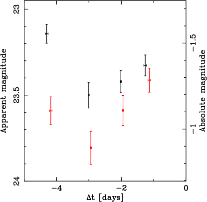
Figure 1: Hubble Space Telescope WFC3/UVIS narrow-band photometry of M31N 2008-12a over the five days before the onset of the 2016 eruption. Red points: F645N “continuum” photometry; black points: F657N “H$\alpha$+[N ii]” photometry. The absolute magnitude assumes a distance to M 31 of 770 kpc (Freedman & Madore, 1990) and reddening toward M31N 2008-12a of $E_{B-V}=0.1$ (DHG17S).

The continuum flux during this period is broadly consistent with the quiescent luminosity of the system (see DHG17P). Therefore, it is unclear whether this behavior is a genuine pre-eruption phenomenon, or related to variability at quiescence with a characteristic time scale of up to a few days, with possible causes being accretion disk flickering, or even orbital modulation. Through constraining the mass donor, DHG17P indicated that the orbital period for the M31N 2008-12a binary should be $\gtrsim 5$ days. Such variation, as shown in Figure 1 would not be inconsistent with that constraint.

3.3 Visible and ultraviolet light curve

Following the 2015 eruption, DHB16 noted that the 2013, 2014, and 2015 eruption light curves were remarkably similar spanning from the $I$-band to the near-UV (redder pass-bands only have data from 2015), see red data points in Figure 2. Based on those observations, DHB16 defined four phases of the light curve: the final rise (Day 0–1) is a regime sparsely populated with data due to the rapid increase to maximum light; the initial decline (Day 1–4) where a exponential decline in flux (linear in magnitude) is observed from the NUV to the near-infrared (see, in particular, the red data points in Figure 3; the plateau (Day 4–8) a relatively flat, but jittery, region of the light curve which is time coincident with the SSS onset; and the final decline (Day $>8$) where a power-law (in flux) decline may be present.

The combined 2013–2015 light curve defined these four phases, the individual light curves from each of those eruptions were also consistent with those patterns (see Figures 2 and 3). A time-resolved SED of the well-covered 2015 eruption was presented by DHB16. Unfortunately, due to severe weather constraints our 2016 campaign did not obtain sufficient simultaneous multi-filter data to compare the SED evolution. However, we find that the 2015 and 2016 light curves are largely consistent (Figure 2) except for the surprising features we will present in the following text.

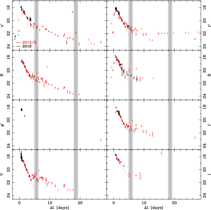
Figure 2: Visible photometry of the past four eruptions of M31N 2008-12a. Black points show the 2016 data (see Table B). The red points indicate combined data from the 2013–2015 eruptions (DWB14, DHS15, DHB16, and TBW14). We show the SSS turn-on/off times of the 2015 eruption as vertical gray lines, with their uncertainties marked by the shaded areas. For the 2013–2015 light curves combined, the inclined gray lines indicate an exponential decay in luminosity during the range of $1\leq\Delta t\leq 4$ days (DHB16).

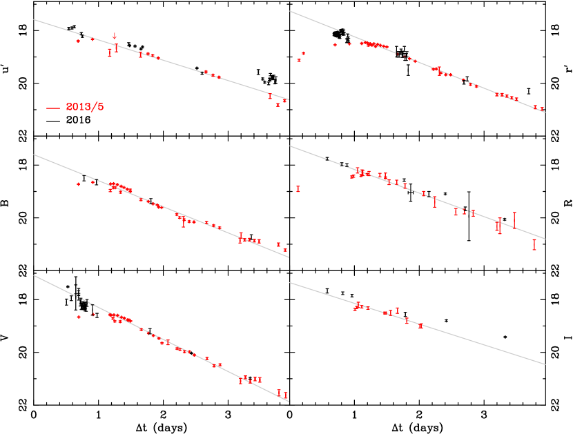
Figure 3: As Figure 2, but focusing on $0\leq t\leq 4$ days. The $i^{\prime}$-band data are excluded as there were no discrepancies between the very limited 2016 $i^{\prime}$ dataset and the extensive dataset from 2013–2015, $g^{\prime}$-band data were excluded as no pre-2016 data exist.

First, we look at the initial decline phase for the 2016 eruption. We examine this region of the light curve first as, in previous eruptions, it has shown the simplest evolution – a linear decline – which was used by DHB16 to tie together the epochs of the 2013, 2014, and 2015 eruptions. But, due to the poor conditions at many of the planned sites, the data here are admittedly sparse, but are generally consistent with the linear behavior seen in the past three eruptions. There may however, be evidence for a deviation, approximately one magnitude upward, toward the end of this phase in the $u^{\prime}$ and $r^{\prime}$-band data at $t\gtrsim 3.6$ days post-eruption.

However, the largest deviation from the 2013–2015 behavior occurs during the final rise phase, between $0\leq t\leq 1$ days. There appears to be a short-lived, ‘cuspy’ feature in the light curves seen through all filters (except the $B$-band where there was limited coverage) and the unfiltered observations (see Figures 2, 3, and 4, which progressively focus on the ‘cusp’). The variation between the peak luminosity of the 2013–2015 eruptions and the 2016 eruption is shown in Table 7, in all useful bands the deviation was significant. The average (across all bands) increase in maximum magnitude was 0.64 mag, or almost twice as luminous as the 2013–2015 eruptions at peak. Notably, this over-luminous peak occurred much earlier than the 2013–2015 peaks. The mean time of peak in 2013–2015 was $t\simeq 1.0$ days (across the $u^{\prime}$, $B$, $R$, $r^{\prime}$, and $I$ filters), whereas the bright cusp in 2016 occurred at $t\simeq 0.65$ days.

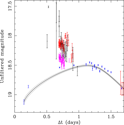
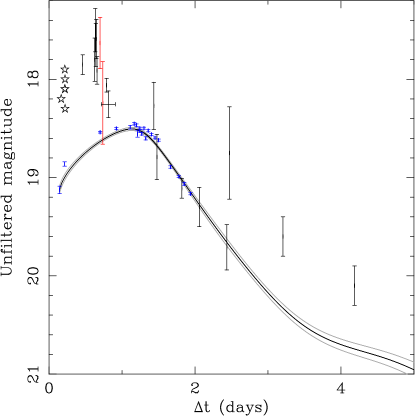
Figure 4: Broad-band and unfiltered photometry of the M31N 2008-12a ‘cusp’. In both sub-plots, the blue points note the combined $r^{\prime}$-band photometry from the 2013, 2014, and 2015 eruptions, with the solid line showing the template 2013–2015 $r^{\prime}$-band light curve and associated uncertainties (see DHB16). Left: Broad-band photometry of the ‘cusp’, of the 2016 eruption of M31N 2008-12a. Red points $r^{\prime}$-band, magenta points $g^{\prime}$-band, and the black points are $V$-band. Right: Here we show a comparison between the unfiltered photometry of the 2010 (red) and 2016 (black) eruptions of M31N 2008-12a, the black stars indicate photometry of the 2016 eruption with no computed uncertainties.

Table 7: Comparison Between the Maximum Observed Magnitudes from the 2013–2015 and 2016 Eruptions of M31N 2008-12a.

Filter	$m_{\mathrm{max}}$ (mag)		‘$\Delta m_{\mathrm{max}}$’
	2013–2015	2016	(mag)
$u^{\prime}$	$18.35\pm 0.03$	$17.85\pm 0.04$	$0.50\pm 0.05$
$B$	$18.67\pm 0.02$	$18.50\pm 0.10$	$0.17\pm 0.10$
$V$	$18.55\pm 0.01$	$17.6$	1.0
$R$	$18.38\pm 0.02$	$17.76\pm 0.05$	$0.62\pm 0.05$
$r^{\prime}$	$18.45\pm 0.01$	$17.98\pm 0.04$	$0.47\pm 0.04$
$I$	$18.31\pm 0.03$	$17.68\pm 0.08$	$0.63\pm 0.09$

The INT and ERAU obtained a series of fast photometry of the 2016 eruption through $g^{\prime}$, $i^{\prime}$ (ERAU only), and $r^{\prime}$-band filters during the final rise phase. Figure 4 (left) compares this photometry with the 2013–2015 $r^{\prime}$-band eruption photometry. This figure clearly illustrates the short-lived, bright, optical ‘cusp’, but also its highly variable nature over a short time-scale with variation of up to 0.4 mag occurring over just 90 minutes. The $(g^{\prime}-r^{\prime})$ color during this period is consistent with the cusp light curve being achromatic. We derive $(g^{\prime}-r^{\prime})_{0}=0.15\pm 0.03$ for the cusp period, which is roughly consistent with the M31N 2008-12a color during the peak of the 2013–2015 eruptions DHB16.

The 2013–2015 eruptions exhibited a very smooth light curve evolution from, essentially, $t=0$ until $t\simeq 4$ days (see in particular the red $r^{\prime}$-band light curve in Figure 3. As well as never being seen before, the bright cusp appears to break this smooth evolution. The 2016 eruption does not just appear more luminous than the observations of 2013–2015, there is evidence of a fundamental change, possibly in the emission mechanism, obscuration, or within the lines.

There are sparse data covering both the plateau and final decline phases. The $R$-band data from 2016 covers the entire plateau phase and is broadly consistent with the slow-jittery decline seen during this phase in the 2013–2015 eruptions. The $u^{\prime}$ and $r^{\prime}$-band data show a departure from the linear early decline around day 3.6, this could indicate an early entry into the plateau, i.e. different behavior in 2016, or simply that the variation seen during the plateau always begins slightly earlier than the assumed 4 day phase transition.

In essence, the 2016 light curves of M31N 2008-12a show a never before seen (but see Section 5.2.3), short-lived, bright cusp at all wavelengths during the final rise phase. There is no further strong evidence of any deviation from previous eruptions – however we again note the sparsity of the later-time data. Possible explanations for the early bright light curve cusp are discussed in Section 5.2.1 and  5.3, and Section 5.2.3 re-examines earlier eruptions for possible indications of similar features.

3.4 Swift and XMM-Newton ultraviolet light curve

During the 2015 eruption we obtained a detailed Swift UVOT light curve through the uvw1 filter (DHB16). For the 2016 eruption our aim was to measure the uvw2 filter magnitudes instead to accumulate additional information on the broad-band SED evolution. With a central wavelength of 1930 Å the uvw2 band is the “bluest” UVOT filter (uvw1 central wavelength is 2600 Å). Therefore, the uvw1 range is more affected by spectral lines, for instance the prominent Mg ii (2800 Å) resonance doublet, than the uvw2 magnitudes (see DHG17S for details). Due to the peculiar properties of the 2016 eruption, a direct comparison between both light curves is now more complex than initially expected.

In Figure 5 we show the 2016 uvw2 light curve compared to the 2015 uvw1 (plus a few uvm2) measurements (DHB16) as well as a few uvw2 magnitudes from the 2014 eruption (HND15, DHS15). The 2016 values are based on individual Swift snapshots (see Table 11) except for the last two data points where we used stacked images (see Table 5). Similarly to the uvw1 light curve in 2015, the uvw2 brightness initially declined linearly with a $t_{2}=2.8\pm 0.2$ d. This is comparable to the 2015 uvw1 value of $t_{2}=2.6\pm 0.2$ d.

From day three onward, the decline slowed down and became less monotonic. Viewed on its own, the UV light curve from this point onward would be consistent with a power-law decline (in flux) with an index of $-1.5\pm 0.2$. However, in light of the well-covered 2015 eruption the 2016 light curve would also be consistent with the presence of three plateaus between (approximately) the days 3–5, 6–8, and 9–12; and with relatively sharp drops of about 1 mag connecting those. Around day 12, when the X-ray flux started to drop (cf. Figure 6) there might even have been a brief rebrightening in the UV before it declined rapidly. The UV source had disappeared by day 16, which is noticeably earlier than in 2015 (in the uvw1 filter). DHG17P presented evidence that the UV–optical flux is dominated by the surviving accretion disk from at least day 13 onward. Therefore, a lower UV luminosity at this stage would imply a lower disk mass accretion rate. It is noteworthy that during the times where the 2014 and 2016 uvw2 measurements overlap they appear to be consistent.

The XMM-Newton OM uvw1 magnitudes are given in Table 6 and included in Figure 5. The two OM measurements appear to be consistently fainter than the Swift UVOT uvw1 data at similar times during the 2015 eruption (cf. DHB16). However, the uncertainties are large and the filter response curves (and instruments) are not perfectly identical. Therefore, we do not consider this apparent difference to have any physical importance. In addition, there is a hint at variability in the uvw1 flux during the first XMM-Newton observation. Of the seven individual OM exposures, the first five can be combined to a uvw1 = $21.3^{+0.3}_{-0.2}$ mag whereas the last two give a $2\sigma$ upper limit of uvw1 $>21.5$ mag. The potential drop in UV flux corresponds to the drop in X-ray flux after the peak in Figure 8. Also here the significance of this fluctuation is low and we only mention it for completeness, in case similar effects will be observed in future eruption.

Figure 5: Swift UVOT uvw2 light curve for the 2016 eruption of M31N 2008-12a  (red) compared to (i) the detailed uvw1 coverage of the 2015 eruption (black; DHB16), (ii) a few uvm2 measurements around the 2015 peak (gray), (iii) the uvw2 magnitudes from the 2014 eruption (blue; DHS15, HND15), and (iv) the 2016 XMM-Newton OM uvw1 magnitudes (cf. Table 6). The last two red data points were derived from stacking multiple images (see Table 5). For better readability we only plot upper limits from individual observations until day 12 are plotted (cf. Tables 4 and 11 for those). Uncertainties are the combined $1\sigma$ systematic and statistical values. Open triangles mark $3\sigma$ upper limits. Day zero is MJD = 57734.32 (see Section 3.1). The dark gray vertical lines indicate the SSS time scales (dashed) and their corresponding uncertainties (dotted) according to Section 3.5.

3.5 Swift XRT light curve

X-ray emission from M31N 2008-12a was first detected at a level of $0.6\pm 0.1$ $\times 10^{-2}$ ct s^-1 on 2016-12-18.101 UT, 5.8 days after the eruption (see Table 4 and also Henze et al., 2016c). Nothing was detected in the previous observation on 2016-12-16.38 UT (day 4.1) with an upper limit of $<0.7$ $\times 10^{-2}$ ct s^-1. Although these numbers are comparable, there is a clear increase of counts at the nova position from the pre-detection observation (zero counts in 1.1 ks) to the detection (more than 30 counts in 3.9 ks). Therefore, we conclude that the SSS phase had started by day 5.8.

For a conservative estimate of the SSS turn-on time (and its accuracy) we use the midpoint between days 4.1 and 5.8 as $t_{\mbox{\small{on}}}=4.9\pm 1.1$ d, which includes the uncertainty of the eruption date. This is consistent with the 2013–2015 X-ray light curves (see Figure 6) for which we estimated turn-on times of $6\pm 1$ d (2013), $5.9\pm 0.5$ d (2014), and $5.6\pm 0.7$ d (2015) using the same method (see HND14, HND15, DHB16). There is no evidence that the emergence of the SSS emission occurred at a different time than in the previous three eruptions.

The duration of the SSS phase, however, was significantly shorter than previously observed (see Figure 6 and Henze et al., 2016d). The last significant detection of X-ray emission in the XRT monitoring was on day 13.9 (Table 4). However, the subsequent 2.9 ks observation on day 15.4 still shows about 4 counts at the nova position which amount to a $2\sigma$ detection (Table 4 gives the $3\sigma$ upper limit). Nothing is visible on day 15.9. Again being conservative we estimate the SSS turn-off time as $t_{\mbox{\small{off}}}=14.9\pm 1.2$ d (including the uncertainty of the eruption date), which is the midpoint between observations 197 and 201 (see Table 4).

In comparison, the SSS turn-off in previous eruptions happened on days $19\pm 1$ (2013), $18.4\pm 0.5$ (2014), and $18.6\pm 0.7$ (2015); all significantly longer than in 2016. The upper limits in Figure 6 and Table 4 demonstrate that we would have detected each of the 2013, 2014, or 2015 light curves during the 2016 monitoring observations, which had similar exposure times (cf. HND14, HND15, and DHB16). Therefore, the short duration of the 2016 SSS phase is real and not caused by an observational bias.

The full X-ray light curve, shown in Figure 6a, is consistent with a shorter SSS phase which had already started to decline before day 12, instead of around day 16 as during the last three years. In a consistent way, the blackbody parametrization in Figure 6b shows a significantly cooler effective temperature ($kT=86\pm 6$ eV) than in 2013–2015 ($kT\sim 115\pm 10$ eV) during days 10–14 (cf. DHB16). As previously, for this plot we fitted the XRT spectra in groups with similar effective temperature.

In contrast to our previous studies of M31N 2008-12a, here our blackbody parameterizations assume a fixed absorption of $N_{\rm H}$ = $0.7$ $\times 10^{21}$ cm^-2 throughout. (The X-ray analysis in DHB16 had explored multiple $N_{\rm H}$ values). This value corresponds to the Galactic foreground. The extinction is based on HST extinction measurements during the 2015 eruption, which are consistent in indicating no significant additional absorption toward the binary system, e.g. from the M 31 disk DHG17S (also see DHB16). These HST spectra were taken about three days before the 2015 SSS phase onset, making it unlikely that the extinction varies significantly during the SSS phase. The new $N_{\mathrm{H}}$, also applied to the 2013–2015 data in Figure 6, affects primarily the absolute blackbody temperature, now reaching almost 140 eV, but not the relative evolution of the four eruptions.

Figure 6a also suggests that the SSS phase in 2016 was somewhat less luminous than in previous eruptions. The early SSS phase of this nova has shown significant flux variability, nevertheless a lower average luminosity is consistent with the XRT light curve binned per Swift snapshot, as shown in Figure 7. A lower XRT count rate would be consistent with the lower effective temperature suggested in Figure 6b. Note, that this refers to the observed characteristics of the SSS; not the theoretically possible maximum photospheric temperature if the hydrogen burning had not extinguished early.

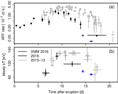
Figure 6: Swift XRT (black) and XMM-Newton EPIC pn (blue) (a) count rates (0.3–1.5 keV) and (b) effective black body temperatures of M31N 2008-12a  during the 2016 eruption compared to the XRT data of the 2013–15 eruptions (gray). Panel a: Triangles indicate upper limits (only shown for 2016 data). Panel b: Sets of observations with similar spectra have been fitted simultaneously assuming a fixed $N_{\rm H}$ = $0.7$ $\times 10^{21}$ cm^-2. The error bars in time represent either the duration of a single observation or the time covering the sets of observations (for panel b and for the last 2016 XRT upper limit in panel a). The deviation of the 2016 eruption from the evolution of past events is clearly visible.

We show the XRT light curve binned per Swift snapshot in Figure 7. As found in previous eruptions (HND14, HND15, DHB16) the early SSS flux is clearly variable. However, here the variability level had already dropped by day $\sim 11$ instead of after day 13 as in previous years. After day 11, the scatter (rms) decreased by a factor of two, which is significant on the 95% confidence level (F-test, $p=0.03$). This change in behavior can be seen better in the detrended Swift XRT count rate light curve in Figure 7b. The faster evolution is consistent with the overall shortening of the SSS duration.

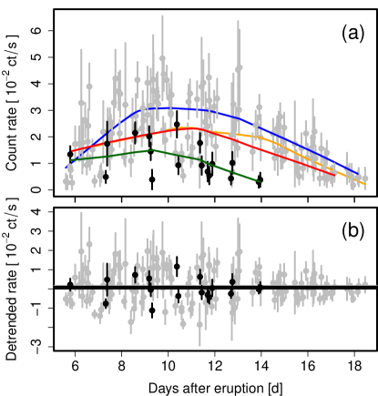
Figure 7: Panel a: The short-term SSS light curve of M31N 2008-12a  derived from all XRT snapshots. The 2016 eruption data is shown in black in contrast to the gray 2013–2015 light curves. Instead of the logarithmic count rate scale in Figure 6 here we use a linear axis. The overlayed green (2016), red (2015), blue (2014), and orange (2013) curves show smoothing fits using local regression. The 2016 light curve is clearly shorter and appears to be less luminous than in 2013–2015. Panel b: Detrended light curves after removing the smoothed trend. The 2016 light curve (black) suggests a drop in variability after day 11, whereas for the 2013–2015 light curves (gray) this drop happened around day 13.

3.6 XMM-Newton EPIC light curves

The XMM-Newton light curves from both pointings show clear variability over time scales of a few 1000 s (Fig. 8). This is an unexpected finding, since the variability in the Swift XRT light curve appeared to have ceased after day 11 (in general agreement with the 2013–15 light curve where this drop in variability occurred slightly later). Instead, we find that the late X-ray light curve around days 14–16 (corresponding to days 18–20 for the “normal” 2013–15 evolution) are still variable by factors of $\sim 5$. The variability is consistent in the EPIC pn and MOS light curves (plotted without scaling in Figure 8).

Even with the lower XRT count rates during the late SSS phase, we would still be able to detect large variations similar to the high-amplitude spike and the sudden drop seen in the first and second EPIC light curve, respectively.

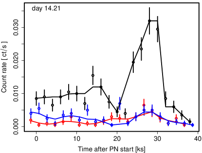
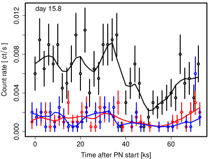
Figure 8: XMM-Newton EPIC light curves for observations 0784000101 (day 14.21; left) and 0784000201 (day 15.80; right) with 2 ks binning. The EPIC pn (black), MOS1 (red), and MOS2 (blue) count rates and corresponding uncertainties are color-coded. The solid lines with the same colours are smoothed fits via locally-weighted polynomial regression (LOWESS).

4 Panchromatic eruption spectroscopy

4.1 Optical spectra

The LT eruption spectra of 2016 are broadly similar to the 2015 (and prior) eruption (see DHB16), with the hydrogen Balmer series being the strongest emission lines (Fig. 9). He i lines are detected at 4471, 5876, 6678 and 7065 Å, along with He ii (4686 Å) blended with N iii (4638 Å). The broad N ii (3) multiplet around 5680 Å is also weakly detected. These emission lines are all typically associated with the He/N spectroscopic class of novae (Williams, 1992). The five LT spectra are shown in Figure 9 (bottom) and cover a similar time frame as those obtained during the 2015 eruption. These spectra are also displayed along with all of the other 2016 spectra at the end of this work in Figure 16.

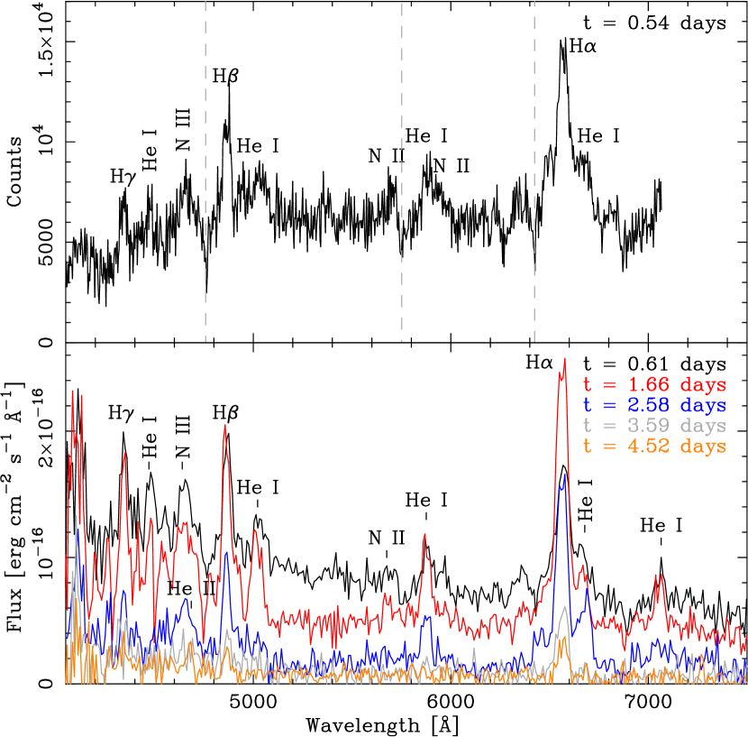
Figure 9: Top: NOT ALFOSC spectrum of M31N 2008-12a, taken 0.54 days after the 2016 eruption, one of the earliest spectra taken of any of the M31N 2008-12a eruptions. The gray dashed lines represent a velocity of $-6250$ km s^-1 with respect the H$\beta$, He i 5876 Å and H$\alpha$. Narrow absorption can be seen at this velocity accompanying the H$\alpha$ and H$\beta$ emission lines, and there is evidence for a similar absorption feature with He i 5876 Å. Bottom: LT spectra of the 2016 eruption, taken between 0.61 and 4.52 days after eruption.

The first 2016 spectrum, taken with NOT/ALFOSC 0.54 days after eruption, shows P Cygni absorption profiles on the H$\alpha$ and H$\beta$ lines. We measure the velocity of the minima of these absorption lines to be at $-6320\pm 160$ and $-6140\pm 200$ km s^-1 for H$\alpha$ and H$\beta$, respectively. This spectrum can be seen in Figure 9 (top), which also shows evidence of a possible weak P Cygni absorption accompanying the He i (5876 Å) line. The first LT spectrum, taken 0.61 days after eruption, also shows evidence of a P Cygni absorption profile on H$\alpha$ (and possibly H$\beta$) at $\sim-6000$ km s^-1.

This is the first time absorption lines have been detected in the optical spectra of M31N 2008-12a. We note that the HST FUV spectra of the 2015 eruption revealed strong, and possibly saturated, P Cygni absorptions still present on the resonance lines of N v, Si iv, and C iv at $t=3.3$ days with terminal velocities in the range 6500–9400 km s^-1, the NUV spectra taken $\sim 1.5$ days later showed only emission lines (DHG17S).

The HET spectrum taken 1.87 d after eruption can be seen in Figure 10, showing that the central emission profiles of the Balmer lines and He i are broadly consistent. Note that the emission around +5000 km s^-1 from the H$\alpha$ rest velocity probably contains a significant contribution from He i (6678 Å). By this time the P Cygni profiles appear to have dissipated.

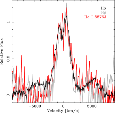
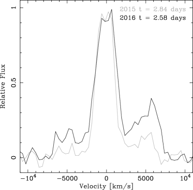
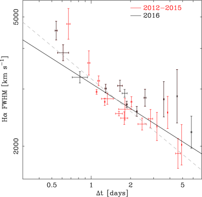
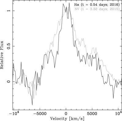
Figure 10: Top left: HET spectrum at day 1.87, showing the similar line structures of H$\alpha$, H$\beta$ and He i (5876 Å). Top right: LT spectra comparing the high-velocity material at day-2.84 of the 2015 eruption to day-2.58 of the 2016 eruption. These are normalized to the lower velocity component peak. Bottom left: FWHM velocity evolution of the H$\alpha$ profile during the 2016 eruption (black), compared to previous eruptions (red). The gray dashed line is a power law of an index of $-1/3$ ($\chi^{2}_{/\mathrm{dof}}=3.7$; Phase II of shocked remnant development) and the solid black line is the best-fit power law with an index of $-0.26\pm$0.04 ($\chi^{2}_{/\mathrm{dof}}=3.6$). Bottom right: comparison between the H$\alpha$ line profile 0.54 days after the 2016 eruption (black) and the N v (1240 Å) profile 3.32 days after the 2015 eruption (gray; see DHG17S). Note that the N v profile has been shifted 500 km s^-1 blueward with respect to H$\alpha$.

Figure 9 clearly shows the existence of high velocity material around the central H$\alpha$ line at day 2.58 of the 2016 eruption. This can be seen in more detail, compared to the 2015 eruption, in Figure 10. Note that, as stated above, the redshifted part of the (2016) profile could be affected by He i (6678 Å), although the weakness of the (isolated) He i line at 7065 Å (see Figure 9) suggests this cannot explain all of the excess flux on this side of the profile. Also note the extremes of the profile indicate a similar velocity (HWZI $\sim$ 6500 to 7000 km s^-1).

The 4.91 day spectrum of the 2015 eruption shows H$\alpha$ and H$\beta$ emission. By comparison, the 2016 4.52-day spectrum also shows a clear emission line from He ii (4686 Å), consistent with the Bowen blend being dominated by He ii at this stage of the eruption. However, we note that this is unlikely to mark a significant difference between 2015 and 2016, as these late spectra typically have very low signal-to-noise ratios. The ARC spectra are shown in Figure 11. The last of these spectra, taken 5.83 d after eruption shows strong He ii (4686 Å) emission. The S/N of the spectrum is relatively low, but the He ii emission appears narrower than the H$\alpha$ line at the same epoch, as seen in Figure 12. At this stage of the eruption we calculate the FWHM of He ii (4686 Å) to be $930\pm 150$ km s^-1, compared to $2210\pm 250$ km s^-1 for H$\alpha$. The ARC spectra have a resolution of $R\sim 1000$, so these two FWHM measurements are not greatly affected by instrumental broadening. Narrow He ii emission has been observed in a number of other novae. It is seen in the Galactic RN U Sco from the time the SSS becomes visible (Mason et al., 2012). Those authors used the changes in the narrow lines with respect to the orbital motion (U Sco is an eclipsing system; Schaefer, 1990) to argue that such emission arises from a reforming accretion disk. In the case of the 2016 eruption of M31N 2008-12a, we clearly observe the SSS at 5.8 d, meaning this final ARC spectrum is taken during the SSS phase. This is consistent with the suggestion that, in M31N 2008-12a, the accretion disk survives the eruption largely intact (DHG17P). In this scenario, the optically thick ejecta prevent us seeing evidence of the disk in our early spectra. We note however, Munari et al. (2014) argued that in the case of KT Eri, there could be two sources of such narrow He ii emission, initially being due to slower moving material in the ejecta, before becoming quickly dominated by emission from the binary itself (as in U Sco) as the SSS enters the plateau phase.

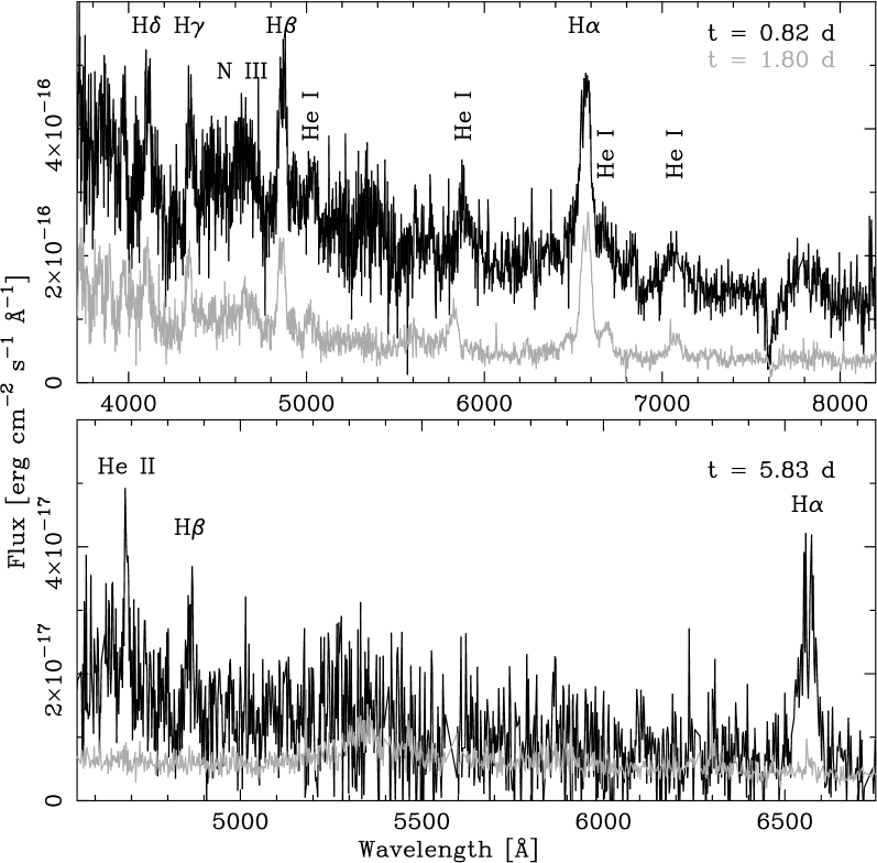
Figure 11: ARC spectra of the 2016 eruption of M31N 2008-12a taken 0.82 and 1.80 d post-eruption (top) and 5.83 d post-eruption (bottom). The bottom panel shows a smaller wavelength range than the top panel, and here the gray line represents the errors for the $t=5.83$ d spectrum.

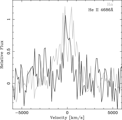
Figure 12: Comparison of H$\alpha$ and He ii 4686 Å emission lines in the $t=5.83$ d ARC spectrum.

DHG17P presented a low S/N, post-SSS spectrum taken 18.8 days after the 2014 eruption of M31N 2008-12a. This spectrum was consistent with that expected from an accretion disk, and H$\beta$ was seen in emission. However, no evidence of the He ii (4686 Å) line was seen in that spectrum. It is possible that the strong He ii line seen in the ARC spectrum arose from the disk but that the transition was excited by the on-going SSS at that time.

As with previous eruptions, the emission line profiles of individual lines showed significant evolution during the 2016 eruption. The FWHM of the main H$\alpha$ emission line (excluding the very high velocity material) narrows from $4540\pm 300$ km s^-1 on day 0.54 to $2210\pm 250$ km s^-1 on day 5.83. The velocity evolution of the 2016 eruption is compared to that of previous eruptions in Figure 10, and is largely consistent. The H$\alpha$ FWHM measurements of all 2016 eruption spectra are given in Table 8

Table 8: FWHM Velocity Measurements of the H$\alpha$ Profile During the 2016 Eruption.

$\Delta t$ (days)	H$\alpha$ FWHM (km s-1)	Instrument
0.54$\pm$0.01	4540$\pm$300	ALFOSC
0.61$\pm$0.06	3880$\pm$220	SPRAT
0.82$\pm$0.11	3260$\pm$130	DIS
1.29$\pm$0.02	3010$\pm$90	HFOSC
1.66$\pm$0.07	3070$\pm$120	SPRAT
1.80$\pm$0.08	2910$\pm$80	DIS
1.87$\pm$0.02	2690$\pm$60	LRS2-B
2.23$\pm$0.02	2560$\pm$90	HFOSC
2.58$\pm$0.05	2820$\pm$170	SPRAT
3.59$\pm$0.02	2790$\pm$350	SPRAT
4.53$\pm$0.02	2850$\pm$540	SPRAT
5.83$\pm$0.05	2210$\pm$250	DIS

4.2 The XMM-Newton EPIC spectra and their connection to the Swift XRT data

The XMM-Newton EPIC spectra for the two observations listed in Table 6 were fitted with an absorbed blackbody model. The three detectors were modeled simultaneously, with only the normalizations free to vary independently. In Table 9 we summarize the best fit parameters and also include a simultaneous fit of all EPIC spectra. The binned spectra, with a minimum of 10 counts per bin, are plotted in Figure 13 together with the model curves. The binning is solely used for visualization here; the spectra were fitted with one-count bins and Poisson (fitting) statistics (Cash, 1979). The $\chi^{2}$ numbers were used as test statistics.

Table 9: Spectral Fits for XMM-Newton Data.

ObsID	$\Delta t^{a}$	$N_{\rm H}$	kT	red. $\chi^{2}$	d.o.f.	kT${}_{0.7}^{b}$	red. $\chi^{2\,\,b}$
	(d)	($10^{21}$ cm-2)	(eV)			(eV)
0784000101	14.21	$2.2^{+0.6}_{-0.7}$	$58^{+8}_{-5}$	1.29	149	$77^{+4}_{-3}$	1.44
0784000201	15.80	$2.7^{+0.6}_{-0.5}$	$45\pm 5$	1.06	140	$68^{+4}_{-3}$	1.35
Both combined	15.01	$2.2\pm 0.4$	$53^{+5}_{-3}$	1.22	291	$73^{+3}_{-2}$	1.42

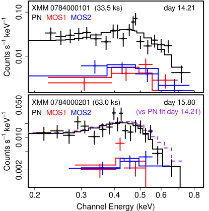
Figure 13: XMM-Newton EPIC spectra of M31N 2008-12a for the two pointings and the three individual (colour-coded) detectors (cf. Table 6). The blackbody fits are shown as solid lines. In the bottom panel the dashed purple line shows the scaled EPIC pn fit from the upper panel, indicating a tentative drop in temperature from $kT=58^{+8}_{-5}$ eV on day 14.21 to $kT=45\pm 5$ eV day 15.8. See Table 9 for details on the spectral fits.

In Table 9 and Figure 13 we immediately see that the two spectra are (a) very similar and (b) contain relatively few spectral counts, leading to a low spectral resolution. The latter point is mainly due to the unexpectedly low flux at the time of the observations, but is also exacerbated by the strong background flaring (cf. Table 6).

In Table 9 we also list a second set of blackbody temperature values (kT_0.7) for the assumption of a fixed $N_{\rm H}$ = $0.7$ $\times 10^{21}$ cm^-2. The purpose of this is to compare these temperatures to the Swift XRT models which share the same assumption (cf. Section 3.5). In both sets of temperatures in Table 9 there is a slight trend toward higher temperatures in the first observation (day 14.21) compared to the second one (day 15.80). While the binned spectra in Figure 13 give a similar impression, which would be consistent with a gradually cooling WD, it needs to be emphasized that this gradient has no high significance because the two (sets of) temperatures are consistent within their $2\sigma-3\sigma$ uncertainties. In fact, the combined fit in Table 9 has reduced $\chi^{2}$ statistics and parameter uncertainties that are similar (the latter even slightly lower) than those of the individual fits.

In Figure 6 the XMM-Newton data points are added to the Swift light curve and temperature evolution. For the conversion from pn to XRT count rate we used the HEASarc WebPIMMS tool (based on PIMMS v4.8d, Mukai, 1993) under the assumption of the best-fit blackbody parameters in the third and fourth column of Table 9.

While the equivalent count rates as well as the temperatures are consistent with the XRT trend of a fading and cooling source there appear to be systematic differences between the XRT and pn rates. This could simply be due to systematic calibration uncertainties between the EPIC pn and the XRT (Madsen et al., 2017). Another reason might be the ongoing flux variability (see Section 3.6). However, it is also possible that deficiencies in the spectral model are preventing a closer agreement between both instruments. We refrain from an attempt to align the pn and XRT count rates because currently there are too many free parameters (e.g., the potential absorption or emission features discussed in DHB16) and insufficient constraints on them. We hope that a future XMM-Newton observation will be able to catch this enigmatic source in a brighter state to shine more (collected) light on its true spectral properties.

5 Discussion

5.1 The relative light curve evolution and the exact eruption date

The precision of the eruption dates for previous outbursts was improved by aligning their light curves, specifically the early, quasi-linear decline (DHB16). For the 2016 eruption, a priori we cannot be certain that this decline phase would be expected to align with previous years because the bright optical peak (Figure 4 left) constitutes an obvious deviation from the established pattern. However, in Figure 2 we find that after the peak feature, most filters appear to decline in the same way as during the previous years. Therefore, we conclude that our estimated eruption date of $\mathrm{MJD}=57734.32\pm 0.17$ (2016-12-12.32 UT) is precise to within the uncertainties – and this brings about a natural alignment of the light curves.

5.2 The peculiarities of the 2016 eruption and their description by theoretical models

From the combined optical and X-ray light curves in Figures 2 and 6 it can be seen that in 2016 (i) the optical peak may have been brighter and (ii) the SSS phase was intrinsically shorter than the previous three eruptions (but began at the same time after eruption). In addition, the gap between the 2015 and 2016 eruptions was longer than usual. Below we study these discrepancies in detail and describe them with updated theoretical model calculations. The following discussion ignores the impact of a possible half-year recurrence (cf. HDK15), the potential dates of which are currently not well constrained (except for the first half of 2016; Henze et al. 2018, in prep.).

The critical advantage of studying a statistically significant number of eruptions from the same nova system is that we can reasonably assume parameters like (accretion and eruption) geometry, metallicity of the accreted material, as well as WD mass, spin, and composition to remain (sufficiently) constant. Therefore, M31N 2008-12a plays a unique role in understanding the variations in nova eruption parameters.

5.2.1 A brighter peak after a longer gap?

This section aims to understand the surprising increase in the optical peak luminosity (the ‘cusp’) by relating it to the delayed eruption date through the theoretical models of Hachisu & Kato (2006); Kato et al. (2014, 2017). While the specifics of our arguments are derived from this particular set of models, we note that all current nova light curve simulations agree on the general line of reasoning (e.g. Yaron et al., 2005; Wolf et al., 2013). We also note that DHG17P found an elevated mass accretion rate to that employed by Kato et al. (2014, 2017), but again the general trends discussed below do not depend on the absolute value of the assumed mass accretion rate.

The gap between the 2015 and 2016 eruptions was 472 d. This is 162 d longer than the 310 d between the 2013 and 2014 eruptions (see Table 1 and Figure 14) and about 35% longer than the median gap (347 d) between the successive eruptions from 2008 to 2015. The well-observed 2015 eruption was very similar to the eruptions in 2013 and 2014 (DHB16) and did not show any indications that would have hinted at a delay in the 2016 eruption (also see DHG17P). This section compares the peculiar 2016 eruption specifically to the 2014 outburst, because we know that the latter was preceded and followed by a “regular” eruption (see Figures 2 and 6, and DHB16). In general, we know that the peak brightness of a nova is higher for a more massive envelope if free-free emission dominates the SED (Hachisu & Kato, 2006).

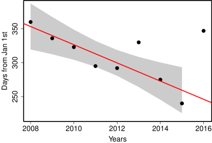
Figure 14: Eruption dates (in days of the year) vs the year from 2008 onward. Individual uncertainties are smaller than the symbols. The best linear model for the 2008-2015 eruptions in shown in red with the 95% uncertainties plotted in gray (cf. DHB16). The .

We consider two specific cases: (1) the mean mass accretion-rate onto the WD ($\dot{M}_{\mathrm{acc}}$) was constant but hydrogen ignition occurs in a certain range around the theoretically expected time and, as a result, the elapsed inter-eruption time was longer in 2016 due to stochastic variance. Alternatively, (2) the mean mass accretion-rate leading up to the 2016 eruption was lower than typical and, as a result, the elapsed time was longer.

(1) If the mean accretion rates prior to the 2014 and 2016 eruptions were the same, then the mass accreted by the WD in 2016 was $\Delta t_{\rm rec}\times\dot{M}_{\rm acc}=162\,{\rm days}\times 1.6\times 10^{-7}\,M_{\sun}$ yr${}^{-1}=0.71\times 10^{-7}\,M_{\sun}$ larger than in 2014. Here we used the mass accretion rate of the $1.38\,M_{\sun}$ model proposed for M31N 2008-12a by Kato et al. (2017). The authors obtained the relation between a wind mass-loss rate and the photospheric temperature (see their Figure 12). The wind mass-loss rate is larger for a lower-temperature envelope, which corresponds to a more extended and more massive envelope.

In Figure 12 of Kato et al. (2017), the rightmost point on the red line corresponds to the peak luminosity of the 2014 eruption. If at this point the envelope mass is higher by $0.71\times 10^{-7}\,M_{\sun}$, then the wind mass-loss rate should increase by $\Delta\log\dot{M}_{\rm wind}\sim 0.08$.

For the free-free emission of novae the optical/IR luminosity is proportional to the square of the wind mass-loss rate (see e.g. Hachisu & Kato, 2006). Thus, the peak magnitude of the optical/IR free-free emission is $2.5\times(\Delta\log\dot{M}_{\rm wind})\times 2=2.5\times 0.08\times 2=0.4$ mag brighter, which is roughly consistent with the increase in the peak magnitudes observed in 2016 in the $V$ and $u^{\prime}$ bands (Figure 2).

However, the time from the optical maximum to $t_{\rm on}$ of the SSS phase should become longer by

$$\Delta t=\frac{\Delta M_{\rm env}}{\Delta\dot{M}_{\rm wind}+\dot{M}_{\rm wind}}\\ =\frac{M_{\rm env}}{\dot{M}_{\rm wind}}\frac{\Delta M_{\rm env}/M_{\rm env}}{\Delta\dot{M}_{\rm wind}/\dot{M}_{\rm wind}+1}\sim\frac{6\times 0.35}{0.2+1}=1.75\text{ days},$$

where $M_{\rm env}$ is the hydrogen-rich envelope mass. This is not consistent with the $t_{\rm on}\sim 6$ days in the 2016 (and 2013–2015) eruptions.

In general, all models agree that a higher-mass envelope would lead to a stronger, brighter eruption with a larger ejected mass (e.g. Starrfield et al., 1998; Yaron et al., 2005; Hachisu & Kato, 2006; Wolf et al., 2013)

(2) For the other case of a lower mean accretion rate, we have estimated the ignition mass of the hydrogen-rich envelope, based on the calculations of Kato et al. (2016, 2017), to be larger by 9% for the 1.35 times longer recurrence period ($0.91\times 1.35=1.23$ yr). Then, the peak magnitude of the free-free emission is $2.5\times(\Delta\log\dot{M}_{\rm wind})\times 2=2.5\times 0.02\times 2=0.1$ mag brighter, but the time from the optical maximum to $t_{\rm on}$ of the SSS phase is longer by only

$$\Delta t=\frac{\Delta M_{\rm env}}{\Delta\dot{M}_{\rm wind}+\dot{M}_{\rm wind}}\\ =\frac{M_{\rm env}}{\dot{M}_{\rm wind}}\frac{\Delta M_{\rm env}/M_{\rm env}}{\Delta\dot{M}_{\rm wind}/\dot{M}_{\rm wind}+1}\sim\frac{6\times 0.09}{0.05+1}=0.5\text{ days}.$$

The peak brightness of the 2016 outburst is about 0.5 days sooner than those in the 2013, 2014, and 2015 eruptions (see Figure 4 left). These two features, the $\sim 0.1$ mag brighter and 0.5 days earlier peak, are roughly consistent with the 2016 eruption except for the $\sim 1$ mag brighter cusp (Figure 4 left).

Observationally, we have shown that the expansion velocities of the 2016 eruption were comparable to previous outbursts (Section 4.1). Together with the comparable SSS turn-on time scale (Section 3.5) this strongly suggests that a similar amount of material was ejected. Therefore, scenario (2) would be preferred here.

It should be emphasized that neither scenario addresses the short-lived, cuspy nature of the peak in contrast to the relatively similar light curves before or after it occurred. The models of Kato et al. (2017) and their earlier studies would predict a smooth light curve with brighter peak and different rise and decline rates.

Ultimately, scenario (2) would also require an explanation of what caused the accretion rate to decrease. The late decline photometry of the 2015 eruption indicated that the accretion disk survived that eruption (DHG17P), however, we have no data from 2013 or 2014 with which to compare the end of that eruption. The similarities of the 2013–2015 eruptions would imply that there was nothing untoward about the 2015 eruption that affected the disk in a different manner to the previous eruptions. Therefore the ‘blame’ probably lies with the donor.

The mass transfer rate in cataclysmic variable stars is known to be variable on time scales from minutes to years (e.g., Warner, 1995, and references therein). The shortest period variations (so called “flickering”), with typical amplitudes of tenths of a magnitude, are believed to be caused by propagating fluctuations in the local mass accretion rate within the accretion disk (Scaringi, 2014). The longer time scale variations that may be relevant to M31N 2008-12a can cause much larger variations in luminosity. In some cases, as in the VY Sculptoris stars, the mass transfer from the secondary star can cease altogether for an extended period of time (e.g., Robinson et al., 1981; Shafter et al., 1985). The VY Scl phenomena is believed to be caused by disruptions in the mass transfer rate caused by star spots on the secondary star drifting underneath the L1 point (e.g., Livio & Pringle, 1994; King & Cannizzo, 1998; Honeycutt & Kafka, 2004). It might be possible that a similar mechanism may be acting in M31N 2008-12a, resulting in mass transfer rate variations sufficient to cause the observed small-scale variability in the recurrence time and potentially even larger “outliers” as in 2016.

5.2.2 A shorter SSS phase

In this section we aim to explain the significantly shorter duration of the 2016 SSS phase in comparison with previous eruptions and with the help of the theoretical X-ray light curve models of Kato et al. (2017).

While a high initial accreted mass at the time of ignition leads to a brighter optical peak (as discussed in the previous section), it does not change the duration of the SSS phase, assuming that the WD envelope settles down to a thermal equilibrium when any wind phase stops. For the same WD mass, a larger accreted mass results in a higher wind mass-loss rate but does not affect the evolution after the maximum photospheric radius has been reached (e.g., Hachisu & Kato, 2006). The shorter SSS duration and thus the shorter duration of the total outburst compared to previous years (Figure 6) therefore needs an additional explanation.

Kato et al. (2017) presented a $1.38~{}M_{\sun}$ WD model with a mean mass accretion-rate of $1.6\times 10^{-7}\,M_{\sun}$ yr^-1 for M31N 2008-12a. They assumed that the mass-accretion resumes immediately after the wind stops, i.e., at the beginning of the SSS phase. The accretion supplies fresh H-rich matter to the WD and substantially lengthens the SSS lifetime, “re-feeding” the SSS, because the mass-accretion rate is the same order as the proposed steady hydrogen shell-burning rate of $\sim 5\times 10^{-7}\,M_{\sun}$ yr^-1. If the accretion does not resume during the SSS phase, or only with a reduced rate, then the SSS duration becomes shorter. This effect is model-independent.

To give a specific example, we calculate the SSS light curves and photospheric temperature evolution for various, post-eruption, mass-accretion rates and plot them in Figure 15. Those are not fits to the data but models that serve the purpose of illustrating the observable effect of a gradually dimished post-eruption re-feeding. The thick solid black lines denote the case of no post-eruption accretion (during the SSS phase). The thin solid black lines represent the case that the mass-accretion resumes post-eruption with $1.6\times 10^{-7}\,M_{\sun}$ yr^-1, just after the optically thick winds stop. The orange dashed, solid red, dotted red lines correspond to the mass-accretion rates of 0.3, 0.65, and 1.5 times the original mass-accretion rate of $1.6\times 10^{-7}\,M_{\sun}$ yr^-1, respectively.

It is clearly shown that a higher post-eruption mass-accretion rate produces a longer SSS phase. Figure 15a shows the X-ray count rates in the 2014 (blue crosses) and 2016 (open black circles) eruptions. The ordinate of the X-ray count rate is vertically shifted to match the theoretical X-ray light curves (cf. Figure 6). The model X-ray flux drops earlier for a lower mass-accretion rate, which could (as a trend) explain the shorter duration of the 2016 SSS phase.

Figure 15b shows the evolution of the blackbody temperature obtained from the Swift spectra with the neutral hydrogen column density of $N_{\rm H}$ = $0.7$ $\times 10^{21}$ cm^-2 (cf. Figure 6 and Section 3.5). The lines show the photospheric temperature of our models. The model temperature decreases earlier for a lower mass-accretion rate. This trend is also consistent with the difference between the 2014 and 2016 eruptions.

Thus, the more rapid evolution of the SSS phase in the 2016 eruption can be partly understood if mass-accretion does not resume soon after the wind stops (zero accretion, thick black line in Figure 15). Note, that the observed change in SSS duration clearly has a larger magnitude than the models (Figure 15). This could indicate deficiencies in the current models and/or that additional effects contributed to the shortening of the 2016 SSS phase. One factor that has an impact on the SSS duration is the chemical composition of the envelope (e.g., Sala & Hernanz, 2005). However, it would be difficult to explain why the abundances of the accreted material would suddenly change from one eruption to the next. In any case, our observations make a strong case for a discontinued re-feeding of the SSS simply by comparing the observed parameters of the 2016 eruption to previous outbursts. The models are consistent with the general trend but need to be improved to be able to simulate the magnitude of the effect.

DHG17P presented evidence that the accretion disk survives eruptions of M31N 2008-12a, the 2015 eruption specifically. In Section 5.2.1 we found that the accretion rate prior to the 2016 eruption might have been lower. If this lower accretion rate was caused by a lower mass-transfer rate from the companion, which is a reasonable possibility, then this would lead to a less massive disk (which was potentially less luminous; see Henze et al. 2018, in prep.). Thus, even if the eruption itself was not stronger than in previous years, as evidenced by the consistent ejection velocities (Section 4.1) and SSS turn-on time scale (Section 3.5), it could still lead to a greater disruption of such a less massive disk. A part of the inner disk mass may be lost, which could prevent or hinder the reestablishment of mass accretion while the SSS is still active.

This scenario can consistently explain the trends toward a brighter optical peak and a shorter SSS phase for the delayed 2016 eruption. Understanding the quantitative magnitude of these changes, and fitting the theoretical light curves more accurately to the observed fluxes, requires additional models that can be tested in future eruptions of M31N 2008-12a. In addition, we strongly encourage the community to contribute alternative interpretations and models that could help us to understand the peculiar 2016 outburst properties.

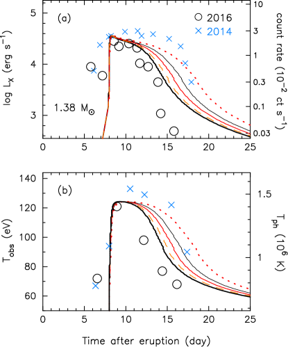
Figure 15: Comparison of the theoretical light curve models with the observational data of the 2016 (open black circles, cf. Tables 4 and 6) and 2014 (blue crosses; cf. HND15) eruptions. The 2014 temperatures were re-analyzed assuming the updated $N_{\rm H}$ = $0.7$ $\times 10^{21}$ cm^-2 (cf. Section 3.5). The theoretical model light curves are based on a $1.38\,M_{\sun}$ WD with a mass accretion rate of $1.6\times 10^{-7}\,M_{\sun}$ yr^-1 (Kato et al., 2017). The five theoretical curves correspond to the cases of no accretion (thick black lines), and factors of 0.3 (dashed orange lines), 0.65 (solid red lines), 1.0 (thin solid black lines), and 1.5 (dotted red lines) times the original mass accretion rate of $1.6\times 10^{-7}\,M_{\sun}$ yr^-1. (a) Theoretical model X-ray light curves (0.3–1.0 keV). (b) Theoretical model photospheric blackbody temperature. There is a clear trend towards a shorter SSS phase for weaker accretion. Improved models are needed to fit the observations with higher accuracy.

5.2.3 Similar features in archival data?

Intriguingly, there is tentative evidence that the characteristic features of the 2016 eruption, namely the bright optical peak and the short SSS phase, might have been present in previous eruptions. Here we discuss briefly the corresponding observational data.

Recall that in X-rays there were two serendipitous detections with ROSAT (Trümper, 1982) in early 1992 and 1993 (see Table 1). White et al. (1995) studied the resulting light curves and spectra in detail. Their Figure 2 shows that in both years the ROSAT coverage captured the beginning of the SSS phase. By chance, the time-axis zero points in these plots are shifted by almost exactly one day with respect to the eruption date as inferred from the rise of the SSS flux; This means that, for example, their day 5 corresponds to day 4 after eruption.

While the 1992 X-ray light curve stops around day eight, the 1993 coverage extends towards day 13 (White et al., 1995). Both light curves show the early SSS variability expected from M31N 2008-12a (cf. Figure 7), but in 1993 the last two data points, near days 12 and 13, have lower count rates than expected from a “regular”, 2015-type eruption (cf. Figure 6). At this stage of the eruption, we would expect the light curve variations to become significantly lower (see also DHB16).

Of course, these are only two data points. However, the corresponding count rate uncertainties are relatively small and at face value these points are more consistent with the 2016-style early X-ray decline than with the 2015 SSS phase which was still bright at this stage (Figure 6). Thus, it is possible that the 1993 eruption had a similarly short SSS phase as the 2016 eruption. The $\sim 341$ d between the 1992 and 1993 eruptions (Table 1), however, are well consistent with the 2008–2015 median of 347 d and suggest no significant delay.

The short-lived, bright, optical cuspy peak seen from the $I$-band to the UV (see Figures 2, 3, and 4 left) from the 2016 eruption may have also been seen in 2010. The 2010 eruption of M31N 2008-12a was not discovered in real-time, but was instead recovered from archival observations (HDK15). The 2010 eruption was only detected in two observations taken just 50 minutes apart, but it appeared up to 0.6 mag brighter than the 2013 and 2014 eruptions (and subsequently 2015). As the 2010 observations were unfiltered, HDK15 noted that the uncertainties on those observations were possibly dominated by calibration systematics – the relative change in brightness is significant. The 2010 photometry is compared with the 2016 photometry in Figure 4 (right), the epoch of the 2010 data was arbitrarily marked as $t=0.7$ d. It is clear from Figure 4 (right), that the bright peak seen in 2016 is not inconsistent with the data from 2010. But it is also clear from Figure 4 (right) that the unfiltered data again illustrate that, other than the cusp itself, the 2016 light curve is similar to those of the 2013–15 eruptions. Indeed, these unfiltered data have much less of a gap around the $t=1$ d peak (as seen in 2013–15) than the filtered data do (see Figures 2 and 3).

However, despite this tentative evidence of a previous ‘cusp’, the 2010 eruption fits the original recurrence period model very well. In fact, it was the eruption that confirmed that original model. So the 2010 eruption appears to have behaved ‘normally’ – but we do note the extreme sparsity of data from 2010. So we must question whether the two deviations from the norm in 2016, the bright cuspy peak, and the X-ray behavior are causally related.

Additionally, we must ask whether the short-lived bright cuspy peak is normal behavior. Figure 4 (left) demonstrates this conundrum well. As noted in Section 5.1, the epoch of the 2016 eruption has been identified simply by the availability of pre-/post-eruption data, $t=0$ has not been tuned (as in 2013–2015) to minimize light curve deviations or based on any other factors. The final rise light curve data from 2013–2015 is sparse, indeed much more data have been collected during this phase in 2016 than in 2013–2015 combined, including the two-color fast-photometry run from the INT – in fact, improving the final rise data coverage was a specified pre-eruption goal for 2016. Figure 4 (left) indicates that should such a short-lived bright peak have occurred in any of 2013, 2014, or 2015, and given our light curve coverage of those eruptions, we may not have detected it. Under the assumption that the eruption times of the 2013–2016 eruptions have been correctly accounted for, we would not have detected a ‘2016 cuspy maximum’ in each of 2013, 2014, or 2015. It is also worth noting that the final rise of the 2016 eruption was poorly covered in the $B$-band (as in all filters in previous years), and no sign of this cuspy behavior is seen in that band! The UV data may shed more light, but we note the unfortunate inconsistency of filters.

In conclusion, we currently don’t have enough final rise data to securely determine whether the 2016 cuspy peak is unusual. However, the planned combination of rapid follow-up and high cadence observations of future eruptions are specifically designed to explore the early time evolution of the eruptions.

5.3 What caused the cusp?

Irrespective of any causal connection between the late 2016 eruption and the newly observed bright cusp, the smooth light curve models can not explain the nature of this new feature. As the cusp ‘breaks’ the previously smooth presentation of the observed light curve and the inherently smooth nature of the model light curves, it must be due to an additional, unconsidered, parameter of the system. Here we briefly discuss a number of possible causes in no particular order.

The cusp could in principle be explained as the shock-breakout associated with the initial thermonuclear runaway, but with evidence of a slower light curve evolution preceding the cusp (see Figure 4 left) the timescales would appear incompatible.

An additional consideration would be the interaction between the ejecta and the donor. Under the assumption of a Roche lobe-filling donor, DHG17P proposed a range of WD–donor orbital separations of $25-44\,R_{\odot}$, those authors also indicated that much larger separations were viable if accretion occured from the wind of the donor. Assuming Roche lobe overflow and typical ejecta velocities at the epoch of the cusp of $\sim 4000$ km s^-1 (see the bottom right plot of Figure 10), one would expect an ejecta–donor interaction to occur 0.02–0.06 days post-eruption (here we have also accounted for the radius of the donor, $R\simeq 14\,R_{\odot}$; DHG17P). With the cusp seemingly occurring 0.65 days post-eruption, the orbital separation would need to be $\sim 330\,R_{\odot}$ ($\sim 1.6$ au). From this we would infer an orbital period in the range $350-490$ days (i.e., $\gtrsim P_{\mathrm{rec}}$), depending on the donor mass, and mass transfer would occur by necessity through wind accretion. We note that the eruption time uncertainty ($\pm 0.17$ d) has little effect on the previous discussion. DHB16, DHG17S, and DHG17P all argued that the system inclination must be low, despite this it is still possible that the observation of such an ejecta–donor interaction may depend upon the orbital phase (with respect to the observer) at the time of eruption.

As a final discussion point, we note that DHB16 and DHG17S both presented evidence of highly asymmetric ejecta; proposing an equatorial component almost in the plane of the sky, and a freely expanding higher-velocity – possibly collimated – polar outflow directed close to the line-of-sight. We also note that the velocity difference between these components may be a factor of three or higher. If we treat these components as effectively independent ejecta, we would therefore expect their associated light curves to evolve at different rates, with the polar component showing the more rapid evolution. Therefore, we must ask whether the ‘normal’ (2013–2015) light curve is that of the ‘bulk’ equatorial ejecta, and the ‘cusp’ is the first photometric evidence of the faster evolving polar ejecta? We note that such proposals have also been put forward to explain multi-peak light curves from other phenomena, for example, kilonovae (see Villar et al., 2017, and the references therein).

5.4 Predicting the date of the next eruption(s)

A consequence of the delayed 2016 eruption is that the dates of the next few eruptions are much more difficult to predict than previously thought. Figure 14 demonstrates how much this surprising delay disrupted the apparently stable trend toward eruptions occurring successively earlier in the year (and Section 5.2 discusses the possible reasons).

Currently, detailed examinations of the statistical properties of the recurrence period distribution are hampered by the relatively small number of nine eruptions, and thereby eight different gaps, since 2008 (cf. Table 1). M31N 2008-12a is the only known nova for which we will overcome this limitation in the near future. For now, we cannot reject the hypothesis that the gaps follow a Gaussian distribution, with Lilliefors (Kolmogorov-Smirnov) test p-value $\sim 0.11$, even with the long delay between 2015 and 2016. The distribution mean (median) is 363 d (347 d), with a standard deviation of 52 d. Thereby, the 472 days prior to the 2016 eruption could indicate a genuine outlier, a skewed distribution, or simply an extreme variation from the mean. It is too early to tell.

In addition, all these gaps of roughly 1 yr length would be affected by the presence of an underlying 6-month period which could dampen the more extreme swings. Of course, the original prediction of a half-year period by HDK15 was partly based on the apparently stable trend toward earlier eruptions since 2008. Comparing this recent trend to the dates of historical X-ray detections in 1992, 1993, and 2001 (HND14), HDK15 found that the most parsimonious explanation for the observed discrepancies between the two regimes would be a 6-month shift. However, the putative 6-month eruption still remains to be found (Henze et al. 2018, in prep.). At present, a single eruption deviating from this pattern does not present sufficient evidence to discard the 6-month scenario. The next (few) eruption date(s) will be crucial in evaluating the recurrence period statistics.

While this manuscript was with the referee, the next eruption was discovered on 2017 Dec 31 (Boyd et al., 2017). The $\sim 384$ d gap between the 2016 and 2017 eruptions is consistent with the pre-2016 eruption pattern. A comprehensive multi-wavelength analysis of the new eruption will be presented in a subsequent work.

6 Summary & Conclusions

1. The 2016 eruption occurred on December 12.32 UT, which was 472 days after the 2015 eruption. Thereby, it appeared to interrupt the general trend of eruptions since 2008 occurring slightly earlier in the year (with $t_{\mathrm{rec}}=347\pm 10$ d).

2. The 2016 eruption light curve exhibited a short lived ‘cuspy’ peak between $0.7\leq t\leq 0.9$ days post-eruption, around 0.5 magnitudes brighter than the smooth peak at $t\simeq 1$ d observed in previous eruptions. This aside, the optical and UV light curve developed in a very similar manner to the 2013/2014/2015 eruptions.

3. The cuspy peak occurs during a previously unsampled portion of the light curve. Therefore we cannot rule out this being a ‘normal’ feature that has previously been missed. There is tentative evidence of a similar occurrence during the 2010 eruption.

4. The first 2016 outburst spectrum, taken 0.54 d after the eruption, was one of the earliest spectra taken of any M31N 2008-12a eruption. From this we identified P Cygni profiles in the optical spectrum of M31N 2008-12a for the first time, indicating an expansion velocity of $\sim 6200$ km s^-1. In addition, a late spectrum taken 5.83 d after eruption revealed narrow He ii emission, possibly arising from the surviving accretion disk. There is however no evidence that the spectroscopic evolution of the 2016 eruption deviated significantly from the behavior in previous years.

5. The Swift XRT light curve deviated significantly from the previous behavior. The flux started to decline around day 11 which is several days earlier than expected. In a consistent way, the evolution of the effective temperature was similar to the 2013–2015 eruptions until day 11 but afterwards decreased significantly earlier. A 100 ks XMM-Newton ToO observation, split into two pointings, managed to characterize the decaying SSS flux and temperature to be consistent with the XRT data and discovered surprising, strong variability at a stage that had previously suggested only marginal variation.

6. The tendency of the changes in recurrence period, optical peak brightness, and SSS duration can be consistently described in early theoretical model calculations. When we assume a lower accretion rate we find that this (i) increases the time between eruptions, (ii) leads to a less-massive disk the disruption of which delays the onset of mass-accretion and shortens the SSS phase, and (iii) increases the ignition mass and thereby the peak magnitude. This scenario will need to be explored in more detail in the future. We also strongly encourage alternative models and interpretations.

Appendix A Additional optical telescopes observing the 2016 eruption of M31N 2008-12a

Among the numerous ground-based observatories that were monitoring the position of M31N 2008-12a for half a year, here we only include those that happened to have weather conditions suitable enough to obtain photometry immediately prior and during the eruption. Regardless of luck with the weather, we are immensely grateful for the hard work and persistence of the entire 2016 monitoring collaboration – the members of which can be found in the author list of this paper.

Below we only list those facilities or telescopes that newly joined our observations of M31N 2008-12a. Details on those instruments that obtained photometry here and already in the 2015 eruption campaign can be found in the Appendix of DHB16. This includes the Ondřejov Observatory (Burke et al., 2016; Hornoch et al., 2016), the Mount Laguna Observatory (MLO; Erdman et al., 2016; Shafter et al., 2016), and the Nayoro Observatory 1.6 m Pirka telescope (Naito et al., 2016).

A.1 Itagaki 50 cm telescope

The 2016 eruption was discovered by Itagaki et al. (2016) using five images (480 s total exposure time) obtained with the 0.5 m f/6 telescope, with a BITRAN BN-52E(KAF-1001E) camera, at the Itagaki Astronomical Observatory, Japan. Additional light curve photometry was first reported in Naito et al. (2016).

A.2 Xingming Observatory Half-Meter-Telescope (HMT)

The confirmation detection and follow-up photometry of M31N 2008-12a were obtained at the Half-Meter-Telescope of the Xingming Observatory, China Itagaki et al. (2016); Tan et al. (2016). The instrument is a 0.508 m aperture, with a focal length of 2.052 m using a QHY11 CCD camera. All images were calibrated using the standard procedure, including flat-field correction, and dark and bias frames using the Maxim DL software. The relative photometry was obtained in PyRAF with an aperture optimized to the seeing of each individual image. The final magnitudes were calibrated using comparison stars from the XPM catalogue (Fedorov et al., 2009).

A.3 Himalayan Chandra Telescope (HCT)

The central 2k$\times$2k region of the Himalayan Faint Object Spectrograph and Camera (HFOSC) mounted on the 2m Himalayan Chandra Telescope (HCT) is used for imaging and gives a field of view of $10^{\prime}\times 10^{\prime}$ at a scale of $0^{\prime\prime}\!\!.296$ pixel^-1.

Photometric observations were made on 2016 December 14.74 UT in the $VRI$ bands, and in the $BVRI$ bands on December 15.67. The images were bias subtracted, and flat field corrected using twilight flats. Instrumental magnitudes were obtained using aperture photometry. An aperture of radius three times FWHM was used. Differential photometry was performed with respect to the stars in the field (DHB16) to estimate the magnitude of the nova.

A.4 Embry Riddle Aeronautical University (ERAU)

Photometry of M31N 2008-12a was obtained at the Embry Riddle Aeronautical University, Florida, with (a) a 24 inch CDK Cassegrain telescope equipped with a SBIG STX 16803 detector, and (b) a 1 m RC telescope equipped with an identical detector. Both telescopes took series of 600s images through Omega SDSS $g^{\prime}$, $r^{\prime}$, and $i^{\prime}$ filters. The total exposure time for each reported magnitude varied between 1–4 hours. The magnitudes were extracted using standard aperture photometric techniques in IRAF (v2.16.1) and calibrated using the DHB16 standard stars in the field. The photometry was first reported in Erdman et al. (2016); Burke et al. (2016); Kaur et al. (2016).

A.5 Danish 1.54 m La Silla

Late-time optical photometric data was collected with the Danish 1.54 m telescope at the ESO La Silla Observatory, operated remotely from Ondřejov, using the Danish Faint Object Spectrograph and Camera (DFOSC) instrument (Hornoch et al., 2016). For each epoch, a series of ten 90s exposures was taken. Standard reduction procedures for raw CCD images were applied (bias subtraction and flat field correction) using the APHOT software (Pravec et al., 1994). Reduced images within the same series were co-added to improve the signal-to-noise ratio and the gradient of the galaxy background was flattened using a spatial median filter via the SIPS program. Photometric measurements of the nova were then performed using aperture photometry in APHOT. Five nearby secondary standard stars from (Massey et al., 2006) were used to photometrically calibrate the magnitudes included in Table B.

A.6 Kiso Observatory

We obtained V-band CCD images with the 1.05 m Schmidt telescope equipped with the Kiso Wide Field Camera (Sako et al., 2012) of the Kiso Observatory, University of Tokyo, Japan. Typical, we took 3 images with 60 s exposure per night. The dark-subtraction and flat-fielding were performed with IRAF (v2.16.1), before image stacking by using SWarp (v2.19.1 Bertin et al., 2002). Photometry of the stacked images was performed via the aperture photometry package in Source Extractor (v2.8.6; Bertin & Arnouts, 1996). We used nearby stars in SDSS, APASS (Henden et al., 2016) and DHB16 for the photometric calibration. The data were first reported in Naito et al. (2016).

A.7 Okayama Astrophysical Observatory

Additional $g^{\prime}$, $R_{\mathrm{C}}$, and $I_{\mathrm{C}}$ band upper limits reported by Naito et al. (2016) were obtained using the 0.5 m, f/6.5 MITSuME telescope (Kotani et al., 2005), equipped with an Apogee Alta U6 camera, of the Okayama Astrophysical Observatory, Japan. We took 10 images with 60 s exposure per night for each of the three bands. Image calibration and photometry followed the same procedure as for the Kiso observatory above.

A.8 Osaka Kyoiku University

Naito et al. (2016) first reported pre-eruption upper limits and light curve photometry obtained by the 0.51 m, f/12 telescope with an Andor DW936N-BV camera of the Osaka Kyoiku University, Japan. These observations were obtained using an $R_{\mathrm{C}}$ filter with 300 s exposure per image. A stack of 14 images were combined using the IRAF task imcombine. We carried out aperture photometry apphot and PSF photometry daophot within the IRAF environment. The source #11 in DHB16 was used as a comparison star.

A.9 Miyaki-Argenteus observatory

Light curve monitoring was performed using a 0.5m f/6.8 telescope, equipped with a SBIG STL1001E camera, at the Miyaki-Argenteus Observatory, Japan (Naito et al., 2016).

A.10 Nayoro Observatory - 0.4 m Meili telescope

We performed observations at Nayoro Observatory, Nayoro, Japan, using the 0.4 m Meili telescope (Meade Schmidt-Cassegrain Telescope) with a SBIG STL-1001E CCD camera (unfiltered or with R-band filter). The obtained images were reduced in a standard manner and stacked using the StellaImage (v6.5) software. Photometry was conducted using Makali’i, a free software provided by National Astronomical Observatory of Japan and AstroArts Inc. for education and research. Magnitudes are measured using an ensemble of comparison stars listed in DHB16. The limiting magnitudes correspond to an S/N of 3 (Naito et al., 2016). The 1.6 m Pirka telescope of the same observatory was also used in this campaign and is described in DHB16.

A.11 New Mexico Skies + AstroCamp Observatory

Additional monitoring data was reported first by (Naito et al., 2016) based on remote observations with the following instruments: (a) a 0.5 m f/4.5 CDK astrograph, with a FLI-PL11002M CCD, at the New Mexico Skies site (Mayhill, NM, USA), (b) a 0.43 m f/6.8 CDK astrograph plus SBIG STL-11000M CCD at the AstroCamp Observatory hosting site (Nerpio, Spain); (c) a 0.32 m f/8.0 CDK astrograph, equipped with a SBIG STXL-6303E CCD, at the AstroCamp Observatory.

A.12 Hankasalmi Observatory (AAVSO OAR)

Pre-eruption upper limits were obtained at Hankasalmi Observatory, Finland using a 0.4 m RC (RCOS) telescope equipped with a SBIG STL-1001E CCD. Typically 25 to 100 unfiltered images with 60 s exposure were obtained per night and stacked using MaxImDL (v4.61). The stacked image was checked for a nova detection by visually using SAOImage DS9 and photometrically using a custom software, with an aperture radius of 6″and a background annulus of 12″–18″. Upper limits were estimated according to the formula $m+2.5\log{s}/3$, where m and s are the magnitude and signal-to-noise, respectively, of comparison star #12 in DHB16.

A.13 CBA Concord Observatory (AAVSO COO)

We observed M31N 2008-12a with the CBA Concord PF29 telescope – a prime focus 0.74 m f/4.36 reflector on an English Cradle mount – located in suburban Concord, CA, USA. Two cameras have been used during this project: an SBIG STL1001E with a clear filter ($1\farcs 52$ pixel) and an SBIG STF 8300M (unfiltered, $0\farcs 34$ pixel^-1, $2\times 2$ binning).

Unfiltered groups of 40–50 images of 15 or 20 s duration were taken and median-combined using the AIP4Win software tool. Typically, 2–4 sets of these groups were averaged within the AAVSO VPHOT online photometry tool. The minimum number of sub-frames was almost always $>100$, usually $\sim 200$. The unfiltered or clear-filter measurements were referenced to the $V$-band comparison stars (see DHB16).

A.14 iTelescope.net T24/T11 (AAVSO COO)

We obtained remote observations with iTelescope.net utilizing (i) the T24 telescope, a Planewave 0.61m CDK Telescope f/6.5 and a FLI PL-9000 CCD camera at the hosting site in Sierra Remote Observatory (SRO), Auberry, CA, USA; and (ii) the T11 telescope, a Planewave 0.5m CDK with a FLI PL-11002M CCD camera at the New Mexico Skies hosting site at Mayfield, NM, USA. Typically three 5 min frames (T24) or three 3 min frames (T11) were obtained in the Luminance filter (a clear filter with UV and IR cut-off). Images were median-combined in AAVSO VPHOT. The detection limits (S/N = 4) are typically 20.7 mag (T24) or 20.2 mag (T11), calibrated using the $R$, $I$ and $V$-band standards in (DHB16). The photometry was estimated in the same way as for the Concord Observatory above.

A.15 Newcastle Observatory (AAVSO CMJA)

We obtained data from the Newcastle Observatory in Newcastle, Ontario, Canada using a 0.40 m Meade Schmidt-Cassegrain (ACF) Telescope working at f/7 and a QSI 516ws CCD camera. The images were obtained in the filters Johnson $V$, Cousins $I_{\mathrm{C}}$, or unfiltered. Most images were a stack of 6 frames, median-combined to minimize cosmic ray effects. At least one imaging run was obtained per night when weather permitted. Occasionally, a second imaging run in the same night (before dawn) was attempted.

All individual images were automatically put through an image processing pipeline for bias, dark, and flat-field calibration, as well as plate-solved to include WCS coordinates before being stacked for analysis. The stack image is viewed in Aladin (v9; Bonnarel et al., 2000; Boch & Fernique, 2014) with the SIMBAD database (Wenger et al., 2000) loaded to accurately locate the target. The detection of the target was compared using the comparison star #8 in DHB16 which has a $V$-band magnitude of 19.087. If the target was not detected (S/N$<3$), the limit was reported as fainter than 19.1 mag.

A.16 Large Binocular Telescope (LBT)

We obtained optical images and photometry of M31N 2008-12a on 2017-01-08.12 UT with the 8.4 m Large Binocular Telescope and Multi-Object Double Spectrograph (MODS2). Images were obtained in the standard SDSS $u^{\prime}g^{\prime}r^{\prime}i^{\prime}z^{\prime}$ filters with a total integration time of 300 s in each of the $g^{\prime}r^{\prime}i^{\prime}z^{\prime}$ filters and 600 s in the $u^{\prime}$ filter at an image scale of 0$\farcs$125 per pixel with a field of view of about $6\arcmin\times 6\arcmin$. Image quality was typically 0$\farcs$8 to 1$\farcs$0 under non–photometric conditions. Bias and twilight–sky flat–field images were obtained in each of the $u^{\prime}g^{\prime}r^{\prime}i^{\prime}z^{\prime}$ filters to facilitate the data reduction. All reductions were performed using IRAF (v2.16).

A.17 West Challow Observatory (AAVSO BDG)

We obtained observations at West Challow Observatory, Oxfordshire, UK, on most clear nights using a 0.35 m Meade Schmidt-Cassegrain Telescope working at f/6.3 with a clear filter and a Starlight Xpress SXVR-H9 CCD camera. Typically 20-30 images with 60 s exposure were recorded, dark-subtracted, flat-fielded and stacked using Astrometrica. Having determined that the nova was not visible in the stacked image at the expected position, the magnitude of the faintest clearly recognizable stellar object in the vicinity of the nova as determined by Astrometrica was reported as the faint magnitude limit for that night. When detected, the magnitude of the nova was measured using the AIP4WIN software and an ensemble of the $V$-band comparison stars listed in DHB16.

A.18 Bernezzo Observatory (AAVSO MAND)

Light curve photometry was obtained at Bernezzo Observatory, Italy, using a 0.25 m f/4 reflector with an Atik 314L CCD and a scale of $1\farcs 33$ per pixel. We stacked 19 individual $V$-band images with 120 s exposure each for a S/N=29.6 detection listed in Table B. The astrometric solution was calibrated through the Astrometrica software. The photometry was extracted using the software FotoDif (v3.95) and calibrated via the AAVSO Variable Star Plotter, which uses comparison starts from DHB16.

A.19 AAVSO PXR

We observed the nova using a 0.4 m SCT telescope, equipped with an SBIG 6303 CCD, located on Haleakala, Hawaii, as part of the LCO group. The exposure times were 60 s with no stacking, flats and darks were applied by LCO. The filter was Johnson $V$ and the photometry used was AIP4WIN using the aperture function. The calibration stars were taken from the APASS catalogue (Henden et al., 2016).

A.20 AAVSO HBB

We obtained light curve photometry using a Meade 0.4-m SCT, with an Astrondon V-band photometric filter and a FLI Proline CCD camera (with 1kx1k back illuminated SITe chip), located at New Smyrna Beach, Florida. Typically, 20–30 sets of 60-s exposures were stacked. The image capture and photometry used the MaximDL v6.14 software. The photometry was calibrated using the comparison starts from DHB16.

A.21 Polaris Observatory

Images were obtained at the Polaris Observatory, Budapest, Hungary, using a 0.25 m f/4 Newtonian reflector with a V filter and an ALCCD5.2 (QHY6) CCD camera. All raw images were processed with gcx v1.3 (dark subtraction and flat field correction and stacking). The integration times were 12 x 180 s. The stacked image was plate-solved with the solve-field tool of astrometry.net. The aperture photometry was performed using IRAF (v2.16.1) and calibrated using the V-band reference stars of DHB16 via the AAVSO VSP.

A.22 Javalambre Observatory (OAJ)

One set of two 400s H$\alpha$ images (central wavelength 6600 Å; FWHM 145 Å) was obtained during the eruption with the JAST/T80 telescope at the Observatorio Astrofisico de Javalambre, in Teruel, owned, managed and operated by the Centro de Estudios de Fisica del Cosmos de Aragon. The aperture photometry was derived using the Source Extractor software (v2.8.6; Bertin & Arnouts, 1996) and calibrated with $R$-band data of the Local Group Galaxies Survey (Massey et al., 2006).

A.23 Observatoire de Haute Provence (AAVSO HDR)

Light curve photometry was obtained via remote observations at the ROTAT and SATINO-2 telescopes, both located at the Observatoire de Haute Provence, France. The telescopes are remotely operated by the “Foundation Interactive Astronomy and Astrophysics”, Germany. ROTAT is a 0.60 m f/3.2 Newtonian reflector used with a clear filter and a SBIG 11000 STL CCD camera. SATINO-2 is a 0.30 m f/6 Schmidt-Cassegrain reflector used with a clear filter and a SBIG ST8-E CCD camera. ROTAT photometry is estimated from a calibrated 600 s guided exposure, while SATINO photometry is based on 19 calibrated and summed 300 s exposures. The photometric analysis was carried out with the MIRA PRO x64 software (v8.012). The photometry was calibrated using the $R$-band magnitudes of the DHB16 comparison stars #11 and #12.

Appendix B Observations of the 2016 eruption of M31N 2008-12a

Tables B and 11 provide full details of the observations of the 2016 eruption of M31N 2008-12a.

Table 10: Complete Dataset of the Visible and Near Infrared Photometric Observations of the 2016 Eruption of M31N 2008-12a.

Date	$\Delta t$	MJD 57,000+		Telescope &	Exposure	Filter	Photometry
(UT)	(days)	Start	End	Instrument	(secs)
2016-12-07.110	-5.210	729.085	729.134	AAVSO COO	$198\times 15$	–	$>20.2$
2016-12-09.807	-2.499	731.807	731.834	AAVSO OAR	$25\times 60$	–	$>20.3$
2016-12-10.164	-2.156	732.154	732.174	AAVSO COO	$7\times 180$	–	$>18.3$
2016-12-10.707	-1.599	732.707	732.734	AAVSO OAR	$25\times 60$	–	$>20.3$
2016-12-10.945	-1.375	732.942	732.948	AAVSO BDG	$8\times 60$	–	$>19.5$
2016-12-11.139	-1.181	733.130	733.175	AAVSO COO	$6\times 180$	–	$>18.4$
2016-12-11.338	-0.982	733.330	733.346	Meili 0.4m	$22\times 30$	–	$>19.0$
2016-12-11.479	-0.841	733.478	733.480	Miyaki-Argenteus	$2\times 60$	–	$>19.0$
2016-12-12.070	-0.250	734.060	734.079	AAVSO COO	$5\times 180$	–	$>19.2$
2016-12-12.091	-0.229			New Mexico Skies	$5\times 120$	–	$>18.3$
2016-12-12.487	+0.167			Itagaki 50cm	480	–	18.2
2016-12-12.536	+0.216			Xingming HMT	60	–	17.9
2016-12-12.537	+0.217			Xingming HMT	60	–	18.1
2016-12-12.538	+0.218			Xingming HMT	60	–	18.1
2016-12-12.539	+0.219			Xingming HMT	60	–	18.0
2016-12-12.540	+0.220			Xingming HMT	60	–	18.3
2016-12-12.782	+0.462			AstroCamp Observatory	$11\times 120$	–	$17.85\pm 0.10$
2016-12-12.946	+0.626			ROTAT	600	–	$17.80\pm 0.22$
2016-12-12.954	+0.634			ROTAT	600	–	$17.50\pm 0.22$
2016-12-12.961	+0.641			ROTAT	600	–	$17.65\pm 0.22$
2016-12-12.968	+0.648			ROTAT	600	–	$17.59\pm 0.20$
2016-12-12.978	+0.658			AstroCamp Observatory	$15\times 120$	–	$17.91\pm 0.14$
2016-12-13.133	+0.813	735.038	735.228	AAVSO COO	$23\times 180$	–	$18.254\pm 0.136$
2016-12-13.109	+0.789			New Mexico Skies	$15\times 120$	–	$18.06\pm 0.07$
2016-12-13.756	+1.436			SATINO-2	$19\times 300$	–	$18.27\pm 0.24$
2016-12-13.798	+1.478			AstroCamp Observatory	$23\times 120$	–	$18.79\pm 0.23$
2016-12-14.139	+1.819			New Mexico Skies	$29\times 120$	–	$19.11\pm 0.10$
2016-12-14.378	+2.058			Itagaki Observatory	$\cdots$	–	$19.3\pm 0.2$
2016-12-14.756	+2.436	736.744	736.765	AAVSO BDG	$30\times 60$	–	$19.71\pm 0.23$
2016-12-14.792	+2.472			ROTAT	600	–	$18.75\pm 0.47$
2016-12-15.525	+3.205			Xingming HMT	$4\times 90$	–	$19.6\pm 0.2$
2016-12-16.449	+4.129	738.448	738.450	Miyaki-Argenteus	$2\times 90$	–	$>20.2$
2016-12-16.506	+4.186			Xingming HMT	$13\times 90$	–	$20.1\pm 0.2$
2016-12-17.133	+4.813	739.083	739.183	AAVSO COO	$297\times 15$	–	$>20.5$
2016-12-17.467	+5.147			Itagaki Observatory	$\cdots$	–	$>20.5$
2016-12-17.539	+5.219			Xingming HMT	$10\times 90$	–	$>20.3$
2016-12-19.110	+6.790	741.098	741.121	AAVSO COO	$334\times 15$	–	$>20.4$
2016-12-19.161	+6.841	741.125	741.204	AAVSO COO	$17\times 300$	–	$>20.7$
2016-12-19.462	+7.142	741.415	741.508	Meili 0.4m	$91\times 30$	–	$>20.5$
2016-12-28.118	+15.798	750.116	750.120	AAVSO COO	300	–	$>19.9$
2016-12-29.110	+16.790	751.048	751.172	AAVSO COO	$334\times 15$	–	$>20.8$
2016-12-13.097	+0.777			MLO	180	$B$	$18.50\pm 0.10$
2016-12-13.289	+0.969			MLO	600	$B$	$18.65\pm 0.10$
2016-12-14.129	+1.809			MLO	1200	$B$	$19.37\pm 0.10$
2016-12-15.679	+3.359			HCT HFOSC	$2\times 900$	$B$	$20.73\pm 0.09$
2016-12-11.368	-0.952	733.365	733.371	Kiso Observatory	$3\times 60$	$V$	$>19.1$
2016-12-12.826	+0.506			Polaris Observatory	$12\times 180$	$V$	$18.094\pm 0.113$
2016-12-12.847	+0.527			AAVSO MAND	$19\times 120$	$V$	$17.511\pm 0.015$
2016-12-12.90	+0.580			Ondřejov 0.65m	1080	$V$	$17.95\pm 0.09$
2016-12-12.969	+0.649			AAVSO PXR	60	$V$	$17.918\pm 0.477$
2016-12-12.970	+0.650			AAVSO PXR	60	$V$	$17.457\pm 0.323$
2016-12-13.012	+0.692			AAVSO HBB	$10\times 60$	$V$	$17.759\pm 0.090$
2016-12-13.014	+0.694			AAVSO HBB	$10\times 60$	$V$	$17.670\pm 0.093$
2016-12-13.016	+0.694			AAVSO HBB	$10\times 60$	$V$	$17.926\pm 0.095$
2016-12-13.038	+0.718			AAVSO HBB	$10\times 60$	$V$	$18.125\pm 0.117$
2016-12-13.047	+0.727			AAVSO HBB	$10\times 60$	$V$	$18.054\pm 0.108$
2016-12-13.055	+0.735			AAVSO HBB	$10\times 60$	$V$	$18.255\pm 0.123$
2016-12-13.066	+0.746			AAVSO HBB	$10\times 60$	$V$	$18.234\pm 0.111$
2016-12-13.079	+0.759			AAVSO HBB	$10\times 60$	$V$	$18.218\pm 0.141$
2016-12-13.092	+0.772			AAVSO HBB	$10\times 60$	$V$	$18.267\pm 0.116$
2016-12-13.105	+0.785			AAVSO HBB	$10\times 60$	$V$	$18.244\pm 0.130$
2016-12-13.112	+0.792			MLO	300	$V$	$18.35\pm 0.08$
2016-12-13.118	+0.798			AAVSO HBB	$10\times 60$	$V$	$18.225\pm 0.127$
2016-12-13.130	+0.810			AAVSO HBB	$10\times 60$	$V$	$18.304\pm 0.140$
2016-12-13.142	+0.822			AAVSO HBB	$10\times 60$	$V$	$18.126\pm 0.132$
2016-12-13.227	+0.907			AAVSO CMJA	$3\times 300$	$V$	$18.394\pm 0.197$
2016-12-13.297	+0.977			MLO	600	$V$	$18.60\pm 0.08$
2016-12-14.115	+1.795			MLO	1200	$V$	$19.20\pm 0.10$
2016-12-14.435	+2.115	736.433	736.437	Kiso Observatory	$2\times 60$	$V$	$>18.2$
2016-12-14.755	+2.435			HCT HFOSC	$2\times 300$	$V$	$20.03\pm 0.02$
2016-12-15.367	+3.047	737.362	737.372	Kiso Observatory	$3\times 60$	$V$	$>20.0$
2016-12-15.660	+3.340			HCT HFOSC	$3\times 420$	$V$	$20.98\pm 0.03$
2016-12-11.382	-0.938	733.379	733.386	Okayama Astrophysical Observatory	$9\times 60$	$R$	$>18.0$
2016-12-11.389	-0.931	733.38	733.40	Osaka Kyoiku University	$5\times 150$	$R$	$>18.8$
2016-12-12.083	-0.237			Palomar $48^{\prime\prime}$	60	$R$	$>19.9$
2016-12-12.90	+0.580			Ondřejov 0.65m	1260	$R$	$17.76\pm 0.05$
2016-12-13.125	+0.805			MLO	300	$R$	$17.97\pm 0.05$
2016-12-13.204	+0.884			MLO	600	$R$	$18.00\pm 0.05$
2016-12-14.088	+1.768			MLO	600	$R$	$18.57\pm 0.05$
2016-12-14.188	+1.868	736.150	736.228	AAVSO COO	$30\times 180$	$R$	$19.045\pm 0.329$
2016-12-14.383	+2.063	736.380	736.387	Okayama Astrophysical Observatory	$9\times 60$	$R$	$>16.3$
2016-12-14.47	+2.150	736.38	736.54	Osaka Kyoiku University	$14\times 300$	$R$	$19.1\pm 0.1$
2016-12-14.722	+2.402			HCT HFOSC	$3\times 150$	$R$	$19.09\pm 0.03$
2016-12-15.031	+2.711			Danish 1.54m	900	$R$	$19.66\pm 0.07$
2016-12-15.087	+2.767			Palomar $48^{\prime\prime}$	60	$R$	$19.94\pm 0.25$
2016-12-15.107	+2.787			Palomar $48^{\prime\prime}$	60	$R$	$>19.8$
2016-12-15.370	+3.050	737.337	737.403	Meili 0.4m	$76\times 60$	$R$	$>20.2$
2016-12-15.504	+3.184	737.433	737.523	Okayama Astrophysical Observatory	$12\times 60$	$R$	$>18.0$
2016-12-15.638	+3.318			HCT HFOSC	$3\times 300$	$R$	$20.06\pm 0.03$
2016-12-16.45	+4.180	738.41	738.49	Osaka Kyoiku University	$20\times 300$	$R$	$>18.7$
2016-12-16.693	+4.373			Ondřejov 0.65m	1800	$R$	$20.4\pm 0.2$
2016-12-17.040	+4.720			Danish 1.54m	900	$R$	$20.74\pm 0.08$
2016-12-17.50	+5.200	739.46	739.54	Osaka Kyoiku University	$19\times 300$	$R$	$>19.3$
2016-12-18.035	+5.715			Danish 1.54m	900	$R$	$20.82\pm 0.09$
2016-12-18.474	+6.154	740.444	740.503	Pirka 1.6m	$5\times 300$	$R$	$>20.6$
2016-12-19.041	+6.721			Danish 1.54m	900	$R$	$21.19\pm 0.15$
2016-12-19.455	+7.135	741.434	741.476	Pirka 1.6m	$7\times 300$	$R$	$>20.5$
2016-12-20.035	+7.715			Danish 1.54m	900	$R$	$21.5\pm 0.2$
2016-12-12.90	+0.580			Ondřejov 0.65m	1080	$I$	$17.68\pm 0.08$
2016-12-13.140	+0.820			MLO	300	$I$	$17.76\pm 0.05$
2016-12-13.283	+0.963			MLO	600	$I$	$17.85\pm 0.05$
2016-12-14.105	+1.785			MLO	600	$I$	$18.56\pm 0.08$
2016-12-14.738	+2.418			HCT HFOSC	$3\times 150$	$I$	$18.80\pm 0.03$
2016-12-15.437	+3.117	737.426	737.447	Pirka 1.6m	$3\times 600$	$I$	$>21.0$
2016-12-15.647	+3.327			HCT HFOSC	$3\times 180$	$I$	$19.42\pm 0.02$
2016-12-19.484	+7.164	741.477	741.484	Pirka 1.6m	$2\times 300$	$I$	$>21.8$
2016-12-28.074	+15.754	750.072	750.076	AAVSO COO	300	$I$	$>17.4$
2016-12-10.850	-1.470	732.845	732.856	LT IO:O	$3\times 300$	$u^{\prime}$	$>22.795$
2016-12-10.925	-1.395	732.920	732.931	LT IO:O	$3\times 300$	$u^{\prime}$	$>22.435$
2016-12-11.008	-1.312	733.002	733.013	LT IO:O	$3\times 300$	$u^{\prime}$	$>22.343$
2016-12-11.903	-0.417	733.897	733.908	LT IO:O	$3\times 300$	$u^{\prime}$	$>22.192$
2016-12-12.862	+0.542	734.858	734.865	LT IO:O	$3\times 180$	$u^{\prime}$	$17.923\pm 0.041$
2016-12-12.910	+0.590	734.906	734.913	LT IO:O	$3\times 180$	$u^{\prime}$	$17.901\pm 0.039$
2016-12-12.947	+0.627	734.944	734.951	LT IO:O	$3\times 180$	$u^{\prime}$	$17.854\pm 0.041$
2016-12-13.055	+0.735	735.052	735.059	LT IO:O	$3\times 180$	$u^{\prime}$	$18.119\pm 0.046$
2016-12-13.071	+0.751	735.067	735.074	LT IO:O	$3\times 180$	$u^{\prime}$	$18.215\pm 0.042$
2016-12-13.786	+1.466	735.783	735.789	LT IO:O	$3\times 180$	$u^{\prime}$	$18.518\pm 0.060$
2016-12-13.800	+1.480	735.797	735.803	LT IO:O	$3\times 180$	$u^{\prime}$	$18.566\pm 0.017$
2016-12-13.884	+1.564	735.880	735.887	LT IO:O	$3\times 180$	$u^{\prime}$	$18.589\pm 0.025$
2016-12-13.975	+1.655	735.972	735.979	LT IO:O	$3\times 180$	$u^{\prime}$	$18.693\pm 0.023$
2016-12-14.000	+1.680	735.997	736.004	LT IO:O	$3\times 180$	$u^{\prime}$	$18.623\pm 0.026$
2016-12-14.839	+2.519	736.835	736.842	LT IO:O	$3\times 180$	$u^{\prime}$	$19.425\pm 0.018$
2016-12-14.919	+2.599	736.916	736.922	LT IO:O	$3\times 180$	$u^{\prime}$	$19.617\pm 0.036$
2016-12-15.787	+3.467	737.784	737.791	LT IO:O	$3\times 180$	$u^{\prime}$	$19.574\pm 0.095$
2016-12-15.854	+3.534	737.853	737.855	LT IO:O	180	$u^{\prime}$	$19.833\pm 0.036$
2016-12-15.885	+3.565	737.882	737.889	LT IO:O	$3\times 180$	$u^{\prime}$	$19.958\pm 0.030$
2016-12-15.946	+3.626	737.943	737.950	LT IO:O	$3\times 180$	$u^{\prime}$	$20.004\pm 0.052$
2016-12-15.959	+3.639	737.955	737.962	LT IO:O	$3\times 180$	$u^{\prime}$	$19.844\pm 0.041$
2016-12-15.966	+3.646	737.963	737.970	LT IO:O	$3\times 180$	$u^{\prime}$	$19.856\pm 0.051$
2016-12-15.973	+3.653	737.971	737.975	LT IO:O	$2\times 180$	$u^{\prime}$	$19.670\pm 0.045$
2016-12-15.990	+3.670	737.986	737.993	LT IO:O	$3\times 180$	$u^{\prime}$	$19.767\pm 0.052$
2016-12-15.997	+3.677	737.994	738.000	LT IO:O	$3\times 180$	$u^{\prime}$	$19.758\pm 0.055$
2016-12-16.005	+3.685	738.001	738.008	LT IO:O	$3\times 180$	$u^{\prime}$	$19.808\pm 0.057$
2016-12-16.012	+3.692	738.009	738.016	LT IO:O	$3\times 180$	$u^{\prime}$	$19.795\pm 0.054$
2016-12-16.024	+3.704	738.020	738.027	LT IO:O	$3\times 180$	$u^{\prime}$	$19.771\pm 0.078$
2016-12-16.041	+3.721	738.038	738.044	LT IO:O	$3\times 180$	$u^{\prime}$	$19.942\pm 0.078$
2016-12-16.058	+3.738	738.055	738.062	LT IO:O	$3\times 180$	$u^{\prime}$	$19.877\pm 0.128$
2016-12-27.887	+15.567	749.876	749.897	LT IO:O	$3\times 600$	$u^{\prime}$	$23.397\pm 0.204$
2016-12-29.856	+17.536	751.845	751.867	LT IO:O	$3\times 600$	$u^{\prime}$	$>18.6$
2016-12-30.843	+18.523	752.832	752.854	LT IO:O	$3\times 600$	$u^{\prime}$	$>21.8$
2017-01-08.121	+26.801			LBT MODS2R	$6\times 100$	$u^{\prime}$	$>23.3$
2016-12-13.010	+0.690			INT WFC	60	$g^{\prime}$	$18.342\pm 0.033$
2016-12-13.012	+0.692			INT WFC	60	$g^{\prime}$	$18.381\pm 0.034$
2016-12-13.015	+0.695			INT WFC	60	$g^{\prime}$	$18.399\pm 0.038$
2016-12-13.017	+0.697			INT WFC	60	$g^{\prime}$	$18.354\pm 0.036$
2016-12-13.020	+0.700			INT WFC	60	$g^{\prime}$	$18.367\pm 0.037$
2016-12-13.022	+0.702			INT WFC	60	$g^{\prime}$	$18.358\pm 0.035$
2016-12-13.024	+0.704			INT WFC	60	$g^{\prime}$	$18.404\pm 0.039$
2016-12-13.027	+0.707			INT WFC	60	$g^{\prime}$	$18.408\pm 0.037$
2016-12-13.029	+0.709			INT WFC	60	$g^{\prime}$	$18.324\pm 0.036$
2016-12-13.032	+0.712			INT WFC	60	$g^{\prime}$	$18.394\pm 0.039$
2016-12-13.034	+0.714			INT WFC	60	$g^{\prime}$	$18.369\pm 0.038$
2016-12-13.036	+0.716			INT WFC	60	$g^{\prime}$	$18.372\pm 0.042$
2016-12-13.039	+0.719			INT WFC	60	$g^{\prime}$	$18.343\pm 0.041$
2016-12-13.041	+0.721			INT WFC	60	$g^{\prime}$	$18.414\pm 0.039$
2016-12-13.044	+0.724			INT WFC	60	$g^{\prime}$	$18.396\pm 0.040$
2016-12-13.046	+0.726			INT WFC	60	$g^{\prime}$	$18.486\pm 0.047$
2016-12-13.051	+0.731			INT WFC	60	$g^{\prime}$	$18.444\pm 0.040$
2016-12-13.053	+0.733			INT WFC	60	$g^{\prime}$	$18.520\pm 0.045$
2016-12-13.055	+0.735			INT WFC	60	$g^{\prime}$	$18.454\pm 0.046$
2016-12-13.058	+0.738			INT WFC	60	$g^{\prime}$	$18.402\pm 0.041$
2016-12-13.060	+0.740			INT WFC	60	$g^{\prime}$	$18.396\pm 0.041$
2016-12-13.062	+0.742			INT WFC	60	$g^{\prime}$	$18.415\pm 0.041$
2016-12-13.065	+0.745			INT WFC	60	$g^{\prime}$	$18.430\pm 0.042$
2016-12-13.067	+0.747			INT WFC	60	$g^{\prime}$	$18.289\pm 0.039$
2016-12-13.070	+0.750			INT WFC	60	$g^{\prime}$	$18.379\pm 0.042$
2016-12-13.072	+0.752			INT WFC	60	$g^{\prime}$	$18.435\pm 0.045$
2016-12-13.075	+0.755			INT WFC	60	$g^{\prime}$	$18.404\pm 0.045$
2016-12-13.078	+0.758			INT WFC	60	$g^{\prime}$	$18.503\pm 0.051$
2016-12-13.081	+0.761			INT WFC	60	$g^{\prime}$	$18.372\pm 0.046$
2016-12-13.084	+0.764			INT WFC	60	$g^{\prime}$	$18.360\pm 0.047$
2016-12-13.086	+0.766			INT WFC	60	$g^{\prime}$	$18.471\pm 0.056$
2016-12-13.089	+0.769			INT WFC	60	$g^{\prime}$	$18.462\pm 0.053$
2016-12-13.092	+0.772			INT WFC	60	$g^{\prime}$	$18.450\pm 0.058$
2016-12-13.096	+0.776			INT WFC	60	$g^{\prime}$	$18.497\pm 0.063$
2016-12-13.170	+0.850			ERAU	$2\times 600$	$g^{\prime}$	$18.42\pm 0.03$
2016-12-14.053	+1.733			ERAU	$6\times 600$	$g^{\prime}$	$19.38\pm 0.07$
2017-01-08.112	+26.792			LBT MODS2R	$3\times 100$	$g^{\prime}$	$>23.1$
2016-12-12.083	-0.237			Palomar $48^{\prime\prime}$	60	$r^{\prime}$	$>19.9$
2016-12-13.007	+0.687			INT WFC	60	$r^{\prime}$	$18.152\pm 0.043$
2016-12-13.008	+0.688			INT WFC	60	$r^{\prime}$	$18.136\pm 0.034$
2016-12-13.011	+0.691			INT WFC	60	$r^{\prime}$	$18.104\pm 0.032$
2016-12-13.014	+0.694			INT WFC	60	$r^{\prime}$	$18.163\pm 0.034$
2016-12-13.016	+0.696			INT WFC	60	$r^{\prime}$	$18.092\pm 0.033$
2016-12-13.018	+0.698			INT WFC	60	$r^{\prime}$	$18.168\pm 0.033$
2016-12-13.021	+0.701			INT WFC	60	$r^{\prime}$	$18.089\pm 0.033$
2016-12-13.023	+0.703			INT WFC	60	$r^{\prime}$	$18.158\pm 0.033$
2016-12-13.026	+0.706			INT WFC	60	$r^{\prime}$	$18.147\pm 0.033$
2016-12-13.028	+0.708			INT WFC	60	$r^{\prime}$	$18.187\pm 0.034$
2016-12-13.030	+0.710			INT WFC	60	$r^{\prime}$	$18.135\pm 0.033$
2016-12-13.033	+0.713			INT WFC	60	$r^{\prime}$	$18.123\pm 0.034$
2016-12-13.035	+0.715			INT WFC	60	$r^{\prime}$	$18.115\pm 0.033$
2016-12-13.038	+0.718			INT WFC	60	$r^{\prime}$	$18.177\pm 0.035$
2016-12-13.040	+0.720			INT WFC	60	$r^{\prime}$	$18.146\pm 0.041$
2016-12-13.042	+0.722			INT WFC	60	$r^{\prime}$	$18.202\pm 0.037$
2016-12-13.045	+0.725			INT WFC	60	$r^{\prime}$	$18.158\pm 0.034$
2016-12-13.047	+0.727			INT WFC	60	$r^{\prime}$	$18.185\pm 0.034$
2016-12-13.052	+0.732			INT WFC	60	$r^{\prime}$	$18.112\pm 0.028$
2016-12-13.054	+0.734			INT WFC	60	$r^{\prime}$	$18.065\pm 0.032$
2016-12-13.056	+0.736			INT WFC	60	$r^{\prime}$	$18.118\pm 0.030$
2016-12-13.059	+0.739			INT WFC	60	$r^{\prime}$	$18.116\pm 0.032$
2016-12-13.061	+0.741			INT WFC	60	$r^{\prime}$	$18.181\pm 0.034$
2016-12-13.064	+0.744			INT WFC	60	$r^{\prime}$	$18.158\pm 0.033$
2016-12-13.066	+0.746			INT WFC	60	$r^{\prime}$	$18.153\pm 0.031$
2016-12-13.069	+0.749			INT WFC	60	$r^{\prime}$	$18.086\pm 0.031$
2016-12-13.071	+0.751			INT WFC	60	$r^{\prime}$	$18.137\pm 0.033$
2016-12-13.073	+0.753			INT WFC	60	$r^{\prime}$	$18.178\pm 0.035$
2016-12-13.077	+0.757			INT WFC	60	$r^{\prime}$	$18.190\pm 0.034$
2016-12-13.079	+0.759			INT WFC	60	$r^{\prime}$	$18.209\pm 0.036$
2016-12-13.083	+0.763			INT WFC	60	$r^{\prime}$	$18.240\pm 0.040$
2016-12-13.085	+0.765			INT WFC	60	$r^{\prime}$	$18.183\pm 0.035$
2016-12-13.088	+0.768			INT WFC	60	$r^{\prime}$	$18.229\pm 0.038$
2016-12-13.090	+0.770			INT WFC	60	$r^{\prime}$	$18.123\pm 0.035$
2016-12-13.094	+0.774			INT WFC	60	$r^{\prime}$	$18.258\pm 0.041$
2016-12-13.103	+0.783			ERAU	600	$r^{\prime}$	$18.02\pm 0.03$
2016-12-13.110	+0.790			ERAU	600	$r^{\prime}$	$18.00\pm 0.04$
2016-12-13.117	+0.797			ERAU	600	$r^{\prime}$	$18.00\pm 0.04$
2016-12-13.125	+0.805			ERAU	600	$r^{\prime}$	$18.08\pm 0.05$
2016-12-13.132	+0.812			ERAU	600	$r^{\prime}$	$18.11\pm 0.05$
2016-12-13.139	+0.819			ERAU	600	$r^{\prime}$	$17.98\pm 0.04$
2016-12-13.146	+0.826			ERAU	600	$r^{\prime}$	$18.13\pm 0.05$
2016-12-13.154	+0.834			ERAU	600	$r^{\prime}$	$18.03\pm 0.05$
2016-12-13.161	+0.841			ERAU	600	$r^{\prime}$	$18.12\pm 0.05$
2016-12-13.201	+0.881			ERAU	600	$r^{\prime}$	$18.39\pm 0.07$
2016-12-13.208	+0.888			ERAU	600	$r^{\prime}$	$18.37\pm 0.07$
2016-12-13.216	+0.896			ERAU	600	$r^{\prime}$	$18.19\pm 0.06$
2016-12-13.223	+0.903			ERAU	600	$r^{\prime}$	$18.31\pm 0.07$
2016-12-13.230	+0.910			ERAU	600	$r^{\prime}$	$18.37\pm 0.07$
2016-12-13.97	+1.650			ERAU	600	$r^{\prime}$	$18.8\pm 0.12$
2016-12-13.99	+1.670			ERAU	600	$r^{\prime}$	$18.9\pm 0.11$
2016-12-14.01	+1.690			ERAU	600	$r^{\prime}$	$18.9\pm 0.11$
2016-12-14.030	+1.710			ERAU	600	$r^{\prime}$	$18.85\pm 0.04$
2016-12-14.04	+1.720			ERAU	600	$r^{\prime}$	$18.8\pm 0.10$
2016-12-14.06	+1.740			ERAU	600	$r^{\prime}$	$18.9\pm 0.12$
2016-12-14.07	+1.750			ERAU	600	$r^{\prime}$	$18.9\pm 0.10$
2016-12-14.09	+1.770			ERAU	600	$r^{\prime}$	$18.7\pm 0.10$
2016-12-14.10	+1.780			ERAU	600	$r^{\prime}$	$19.0\pm 0.13$
2016-12-14.12	+1.800			ERAU	600	$r^{\prime}$	$19.0\pm 0.13$
2016-12-14.13	+1.810			ERAU	600	$r^{\prime}$	$18.9\pm 0.10$
2016-12-14.15	+1.830			ERAU	600	$r^{\prime}$	$19.5\pm 0.20$
2016-12-15.01	+2.690			ERAU	$6\times 600$	$r^{\prime}$	$19.96\pm 0.07$
2016-12-15.06	+2.740			ERAU	$11\times 600$	$r^{\prime}$	$19.83\pm 0.08$
2016-12-16.01	+3.690			ERAU	$6\times 600$	$r^{\prime}$	$20.30\pm 0.10$
2016-12-16.99	+4.670			ERAU	$10\times 600$	$r^{\prime}$	$20.85\pm 0.13$
2016-12-17.08	+4.760			ERAU	$13\times 600$	$r^{\prime}$	$21.08\pm 0.15$
2016-12-18.00	+5.680			ERAU	$19\times 600$	$r^{\prime}$	$21.35\pm 0.14$
2017-01-08.112	+26.792			LBT MODS2R	$3\times 100$	$r^{\prime}$	$>22.8$
2016-12-13.185	+0.865			ERAU	$2\times 600$	$i^{\prime}$	$18.08\pm 0.05$
2016-12-13.99	+1.670			ERAU	600	$i^{\prime}$	$19.0\pm 0.14$
2016-12-14.01	+1.690			ERAU	600	$i^{\prime}$	$18.8\pm 0.12$
2016-12-14.04	+1.720			ERAU	600	$i^{\prime}$	$18.9\pm 0.13$
2016-12-14.06	+1.740			ERAU	600	$i^{\prime}$	$19.01\pm 0.14$
2016-12-14.07	+1.750			ERAU	600	$i^{\prime}$	$18.8\pm 0.11$
2016-12-14.09	+1.770			ERAU	600	$i^{\prime}$	$18.8\pm 0.12$
2016-12-14.10	+1.780			ERAU	600	$i^{\prime}$	$19.1\pm 0.14$
2016-12-14.12	+1.800			ERAU	600	$i^{\prime}$	$18.7\pm 0.10$
2016-12-14.13	+1.810			ERAU	600	$i^{\prime}$	$19.0\pm 0.14$
2016-12-14.15	+1.830			ERAU	600	$i^{\prime}$	$19.1\pm 0.17$
2017-01-08.118	+26.798			LBT MODS2R	$3\times 100$	$i^{\prime}$	$>22.7$
2017-01-08.123	+26.803			LBT MODS2R	$3\times 100$	$z^{\prime}$	$>22.5$
2016-12-07.976	-4.344	729.971	729.981	HST WFC3/UVIS	898	F657W	$23.074\pm 0.092$
2016-12-08.041	-4.279	730.036	730.046	HST WFC3/UVIS	898	F657W	$23.350\pm 0.107$
2016-12-08.053	-4.267	730.048	730.058	HST WFC3/UVIS	898	F657W	$22.986\pm 0.088$
2016-12-09.300	-3.020	731.295	731.305	HST WFC3/UVIS	898	F657W	$23.527\pm 0.130$
2016-12-09.312	-3.008	731.307	731.317	HST WFC3/UVIS	898	F657W	$23.634\pm 0.143$
2016-12-09.324	-2.996	731.319	731.329	HST WFC3/UVIS	898	F657W	$23.343\pm 0.117$
2016-12-10.293	-2.027	732.288	732.299	HST WFC3/UVIS	898	F657W	$23.356\pm 0.113$
2016-12-10.305	-2.015	732.300	732.311	HST WFC3/UVIS	898	F657W	$23.542\pm 0.122$
2016-12-10.317	-2.003	732.312	732.322	HST WFC3/UVIS	898	F657W	$23.361\pm 0.102$
2016-12-11.022	-1.298	733.016	733.027	HST WFC3/UVIS	898	F657W	$23.390\pm 0.109$
2016-12-11.087	-1.233	733.081	733.092	HST WFC3/UVIS	898	F657W	$23.237\pm 0.098$
2016-12-11.099	-1.221	733.093	733.104	HST WFC3/UVIS	898	F657W	$23.352\pm 0.110$
2016-12-12.794	+0.474			OAJ	$2\times 400$	H$\alpha$	$17.34\pm 0.17$
2016-12-17.048	+4.728	739.042	739.053	HST WFC3/UVIS	898	F657W	$19.386\pm 0.012$
2016-12-17.060	+4.740	739.055	739.065	HST WFC3/UVIS	898	F657W	$19.385\pm 0.012$
2016-12-17.113	+4.793	739.108	739.118	HST WFC3/UVIS	898	F657W	$19.267\pm 0.011$
2016-12-08.107	-4.213	730.102	730.113	HST WFC3/UVIS	935	F645W	$23.529\pm 0.130$
2016-12-08.120	-4.200	730.114	730.125	HST WFC3/UVIS	935	F645W	$23.489\pm 0.130$
2016-12-08.174	-4.146	730.168	730.179	HST WFC3/UVIS	935	F645W	$23.778\pm 0.167$
2016-12-09.365	-2.955	731.360	731.371	HST WFC3/UVIS	935	F645W	$23.780\pm 0.162$
2016-12-09.378	-2.942	731.372	731.383	HST WFC3/UVIS	935	F645W	$24.182\pm 0.208$
2016-12-09.390	-2.930	731.385	731.396	HST WFC3/UVIS	935	F645W	$23.379\pm 0.134$
2016-12-10.359	-1.961	732.353	732.364	HST WFC3/UVIS	935	F645W	$23.792\pm 0.187$
2016-12-10.371	-1.949	732.365	732.376	HST WFC3/UVIS	935	F645W	$23.482\pm 0.152$
2016-12-10.383	-1.937	732.378	732.389	HST WFC3/UVIS	935	F645W	$23.521\pm 0.127$
2016-12-11.153	-1.167	733.148	733.158	HST WFC3/UVIS	935	F645W	$23.591\pm 0.137$
2016-12-11.165	-1.155	733.160	733.171	HST WFC3/UVIS	935	F645W	$23.189\pm 0.104$
2016-12-11.219	-1.101	733.214	733.225	HST WFC3/UVIS	935	F645W	$23.457\pm 0.127$
2016-12-17.126	+4.806	739.120	739.131	HST WFC3/UVIS	935	F645W	$20.529\pm 0.023$
2016-12-17.180	+4.860	739.174	739.185	HST WFC3/UVIS	935	F645W	$20.290\pm 0.020$
2016-12-17.192	+4.872	739.187	739.197	HST WFC3/UVIS	935	F645W	$20.625\pm 0.024$

Note. — This is an updated version of Table 1 as it was published by Tang et al. (2014), Darnley et al. (2015c), Henze et al. (2015a), and Darnley et al. (2016d). Here we add the 2016 eruption information.

References. — (1) White et al. (1995), (2) Henze et al. (2015a), (3) Williams et al. (2004), (4) Nishiyama & Kabashima (2008), (5) Tang et al. (2014), (6) Korotkiy & Elenin (2011), (7) Barsukova et al. (2011), (8) Darnley et al. (2015c), (9) Nishiyama & Kabashima (2012), (10) Shafter et al. (2012), (11) Henze et al. (2014a), (12) Tang et al. (2013), (13) Darnley et al. (2014), (14) Darnley et al. (2016d), (15) Henze et al. (2015d), (16) Darnley et al. (2015a), (17) Darnley et al. (2015b), (18) Henze et al. (2015e), (19) this paper, (20) Itagaki (2016), (21) Itagaki et al. (2016), (22) Henze et al. (2016a), (23) Henze et al. (2016c), (24) Boyd et al. (2017), (25) Henze et al. (2018a), (26) Henze et al. (2018b), (27) Darnley et al. (2018).

References. — (a) Darnley & Hounsell (2016).

Note. — The time since eruption assumes an eruption date of 2016 December 12.32 UT. The error bars do not include the systematic error in this eruption date, but represent the total exposure time/time between combined exposures of a given epoch.

Note. — (Includes all observations from $t\sim 7$ days before the eruption until $t\sim 30$ days post-eruption. This table is available in its entirety in machine-readable form.)

References. — (a) Naito et al. (2016), (b) Itagaki et al. (2016), (c) Tan et al. (2016), (d) Shafter et al. (2016), (e) Burke et al. (2016), (f) Hornoch et al. (2016), (g) Darnley et al. (2016c), (h) Darnley (2016), (i) Erdman et al. (2016), (j) Kaur et al. (2016), (k) Darnley & Hounsell (2016).

Table 11: Individual Swift Snapshots of the Observations in Table 4. Plotted in Figure 7.

ObsID_part	Expa	Dateb	MJDb	$\Delta t^{c}$	uvw2d	Rate
	[ks]	[UT]	[d]	[d]	[mag]	[$10^{-2}$ ct s-1]
00032613183_1	2.26	2016-12-12.65	57734.65	0.33	$16.56\pm 0.08$	$<0.5$
00032613183_2	1.73	2016-12-12.72	57734.72	0.40	$16.61\pm 0.08$	$<0.6$
00032613184_1	0.95	2016-12-13.19	57735.19	0.87	$16.95\pm 0.09$	$<1.2$
00032613184_2	1.07	2016-12-13.59	57735.59	1.27	$17.25\pm 0.09$	$<1.0$
00032613184_3	1.13	2016-12-13.71	57735.72	1.40	$17.37\pm 0.09$	$<1.1$
00032613184_4	0.99	2016-12-13.78	57735.79	1.47	$17.36\pm 0.10$	$<1.6$
00032613185_1	1.35	2016-12-14.25	57736.26	1.94	$17.78\pm 0.10$	$<0.8$
00032613185_2	0.21	2016-12-14.33	57736.33	2.01	$17.79\pm 0.16$	$<5.3$
00032613185_3	1.26	2016-12-14.38	57736.39	2.07	$17.88\pm 0.10$	$<0.9$
00032613185_4	0.90	2016-12-14.45	57736.45	2.13	$17.89\pm 0.11$	$<1.3$
00032613186_1	1.31	2016-12-15.64	57737.65	3.33	$18.61\pm 0.12$	$<1.0$
00032613186_2	0.58	2016-12-15.92	57737.92	3.60	$18.94\pm 0.19$	$<1.9$
00032613186_3	1.35	2016-12-15.97	57737.97	3.65	$18.37\pm 0.11$	$<0.8$
00032613188_1	1.10	2016-12-16.38	57738.38	4.06	$18.65\pm 0.13$	$<1.0$
00032613189_1	1.71	2016-12-18.10	57740.10	5.78	$19.27\pm 0.15$	$1.3\pm 0.3$
00032613189_2	1.64	2016-12-18.16	57740.17	5.85	$19.06\pm 0.14$	$<0.5$
00032613189_3	0.56	2016-12-18.23	57740.23	5.91	$19.71\pm 0.32$	$<2.1$
00032613190_1	1.36	2016-12-19.49	57741.50	7.18	$19.67\pm 0.21$	$<1.0$
00032613190_2	0.63	2016-12-19.56	57741.57	7.25	$20.02\pm 0.35$	$<1.7$
00032613190_3	1.65	2016-12-19.62	57741.63	7.31	$19.96\pm 0.23$	$0.5\pm 0.2$
00032613190_4	0.42	2016-12-19.69	57741.69	7.37	$>19.8$	$1.7\pm 0.8$
00032613191_1	1.65	2016-12-20.88	57742.89	8.57	$20.49\pm 0.33$	$2.2\pm 0.4$
00032613191_2	0.24	2016-12-20.97	57742.97	8.65	-	$1.0\pm 0.9$
00032613191_3	0.11	2016-12-20.97	57742.98	8.66	$>19.0$	$<9.9$
00032613192_1	1.67	2016-12-21.49	57743.49	9.17	$>20.8$	$1.9\pm 0.4$
00032613192_2	1.61	2016-12-21.55	57743.56	9.24	$20.62\pm 0.35$	$1.4\pm 0.3$
00032613192_3	0.69	2016-12-21.62	57743.62	9.30	$>20.2$	$0.4\pm 0.4$
00032613193_1	1.22	2016-12-22.68	57744.69	10.37	$20.21\pm 0.30$	$2.5\pm 0.5$
00032613193_2	1.32	2016-12-22.74	57744.75	10.43	$20.33\pm 0.32$	$0.9\pm 0.3$
00032613194_1	1.71	2016-12-23.67	57745.68	11.36	$20.71\pm 0.38$	$1.8\pm 0.4$
00032613194_2	1.24	2016-12-23.75	57745.75	11.43	$>20.6$	$0.9\pm 0.3$
00032613195_1	0.92	2016-12-24.00	57746.01	11.69	$19.87\pm 0.29$	$0.7\pm 0.4$
00032613195_2	0.90	2016-12-24.07	57746.08	11.76	$>20.4$	$0.7\pm 0.4$
00032613195_3	0.90	2016-12-24.20	57746.21	11.89	$>20.4$	$1.0\pm 0.4$
00032613195_4	0.19	2016-12-24.34	57746.34	12.02	$>19.2$	$<6.0$
00032613196_1	1.60	2016-12-25.00	57747.01	12.69	$>20.7$	$0.4\pm 0.2$
00032613196_2	0.99	2016-12-25.07	57747.07	12.75	$>20.4$	$1.0\pm 0.4$
00032613196_3	0.21	2016-12-25.13	57747.14	12.82	$>19.4$	$<5.4$
00032613197_1	1.37	2016-12-26.20	57748.20	13.88	$>20.6$	$0.3\pm 0.2$
00032613197_2	1.35	2016-12-26.26	57748.27	13.95	$>20.6$	$0.4\pm 0.3$
00032613198_1	1.60	2016-12-27.72	57749.73	15.41	$>20.7$	$<0.7$
00032613198_2	1.25	2016-12-27.79	57749.79	15.47	$>20.5$	$<1.0$
00032613199_1	1.69	2016-12-28.19	57750.19	15.87	$>20.7$	$<0.5$
00032613199_2	1.56	2016-12-28.26	57750.26	15.94	$>20.6$	$<0.8$
00032613200_1	1.49	2016-12-29.45	57751.46	17.14	$>20.7$	$<0.7$
00032613200_2	0.88	2016-12-29.52	57751.53	17.21	$>20.3$	$<1.3$
00032613200_3	0.30	2016-12-29.65	57751.66	17.34	$>19.6$	$<3.4$
00032613201_1	0.79	2016-12-30.05	57752.05	17.73	$>20.2$	$<1.4$
00032613201_2	0.91	2016-12-30.12	57752.12	17.80	-	$<1.2$
00032613201_3	0.69	2016-12-30.46	57752.46	18.14	$>20.2$	$<1.6$
00032613201_4	0.68	2016-12-30.65	57752.65	18.33	$>20.1$	$<1.7$
00032613202_1	1.65	2016-12-31.58	57753.58	19.26	$>20.7$	$<0.8$
00032613202_2	1.25	2016-12-31.65	57753.66	19.34	$>20.6$	$<0.9$

Appendix C Spectra of the 2016 eruption of M31N 2008-12a

Figure 16 presents all the spectra following the 2016 eruption of M31N 2008-12a, as recorded in Table 3. As it was not possible to obtain an absolute flux calibration of all the spectra, here they are presented with arbitrary flux.

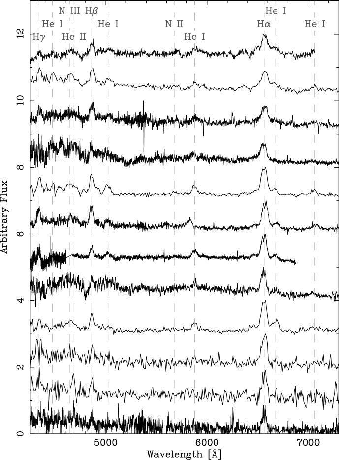
Figure 16: All spectra of the 2016 eruption of M31N 2008-12a. The figure shows the spectra in date order (see Table 3) from the 0.54 d ALFOSC/NOT spectrum at the top to the 5.83 d DIS/ARC spectrum at the bottom. The wavelengths of prominent lines are indicated.

References

- Arnaud (1996) Arnaud, K. A. 1996, in Astronomical Society of the Pacific Conference Series, Vol. 101, Astronomical Data Analysis Software and Systems V, ed. G. H. Jacoby & J. Barnes, 17–+
- Balucinska-Church & McCammon (1992) Balucinska-Church, M., & McCammon, D. 1992, ApJ, 400, 699
- Barsukova et al. (2011) Barsukova, E., Fabrika, S., Hornoch, K., et al. 2011, ATel, 3725, 1
- Bertin & Arnouts (1996) Bertin, E., & Arnouts, S. 1996, A&AS, 117, 393
- Bertin et al. (2002) Bertin, E., Mellier, Y., Radovich, M., et al. 2002, in Astronomical Society of the Pacific Conference Series, Vol. 281, Astronomical Data Analysis Software and Systems XI, ed. D. A. Bohlender, D. Durand, & T. H. Handley, 228
- Boch & Fernique (2014) Boch, T., & Fernique, P. 2014, in Astronomical Society of the Pacific Conference Series, Vol. 485, Astronomical Data Analysis Software and Systems XXIII, ed. N. Manset & P. Forshay, 277
- Bode & Evans (2008) Bode, M. F., & Evans, A., eds. 2008, Cambridge Astrophysics Series, Vol. 43, Classical Novae, 2nd Edition (Cambridge: Cambridge University Press)
- Bode et al. (2016) Bode, M. F., Darnley, M. J., Beardmore, A. P., et al. 2016, ApJ, 818, 145
- Bonnarel et al. (2000) Bonnarel, F., Fernique, P., Bienaymé, O., et al. 2000, A&AS, 143, 33
- Boyd et al. (2017) Boyd, D., Hornoch, K., Henze, M., et al. 2017, The Astronomer’s Telegram, 11116
- Breeveld et al. (2011) Breeveld, A. A., Landsman, W., Holland, S. T., et al. 2011, in American Institute of Physics Conference Series, Vol. 1358, American Institute of Physics Conference Series, ed. J. E. McEnery, J. L. Racusin, & N. Gehrels, 373–376
- Brown et al. (2013) Brown, T. M., Baliber, N., Bianco, F. B., et al. 2013, PASP, 125, 1031
- Burke et al. (2016) Burke, D., Kaur, A., Oswalt, T., et al. 2016, ATel, 9861
- Burrows et al. (2005) Burrows, D. N., Hill, J. E., Nousek, J. A., et al. 2005, Space Sci. Rev., 120, 165
- Cash (1979) Cash, W. 1979, ApJ, 228, 939
- Chandrasekhar (1931) Chandrasekhar, S. 1931, ApJ, 74, 81
- Chonis et al. (2014) Chonis, T. S., Hill, G. J., Lee, H., Tuttle, S. E., & Vattiat, B. L. 2014, in Proc. SPIE, Vol. 9147, Ground-based and Airborne Instrumentation for Astronomy V, 91470A
- Chonis et al. (2016) Chonis, T. S., Hill, G. J., Lee, H., et al. 2016, in Proc. SPIE, Vol. 9908, Ground-based and Airborne Instrumentation for Astronomy VI, 99084C
- Darnley (2016) Darnley, M. J. 2016, ATel, 9910
- Darnley (2017) Darnley, M. J. 2017, in Astronomical Society of the Pacific Conference Series, Vol. 509, 20th European White Dwarf Workshop, ed. P.-E. Tremblay, B. Gaensicke, & T. Marsh, 515
- Darnley et al. (2018) Darnley, M. J., Healy, M. W., Henze, M., & Williams, S. C. 2018, The Astronomer’s Telegram, 11149
- Darnley et al. (2015a) Darnley, M. J., Henze, M., Shafter, A. W., & Kato, M. 2015a, ATel, 7964, 1
- Darnley et al. (2015b) —. 2015b, ATel, 7965, 1
- Darnley & Hounsell (2016) Darnley, M. J., & Hounsell, R. 2016, ATel, 9874
- Darnley et al. (2016a) Darnley, M. J., Kuin, N. P. M., Page, K. L., et al. 2016a, ATel, 8587
- Darnley et al. (2016b) Darnley, M. J., Rodriguez-Gil, P., & Prieto-Arranz, J. 2016b, ATel, 9852
- Darnley et al. (2014) Darnley, M. J., Williams, S. C., Bode, M. F., et al. 2014, A&A, 563, L9
- Darnley et al. (2016c) Darnley, M. J., Williams, S. C., Henze, M., et al. 2016c, ATel, 9906
- Darnley et al. (2007) Darnley, M. J., Kerins, E., Newsam, A., et al. 2007, ApJ, 661, L45
- Darnley et al. (2015c) Darnley, M. J., Henze, M., Steele, I. A., et al. 2015c, A&A, 580, A45
- Darnley et al. (2016d) Darnley, M. J., Henze, M., Bode, M. F., et al. 2016d, ApJ, 833, 149
- Darnley et al. (2017a) Darnley, M. J., Hounsell, R., O’Brien, T. J., et al. 2017a, ArXiv e-prints, arXiv:1712.04872
- Darnley et al. (2017b) Darnley, M. J., Hounsell, R., Godon, P., et al. 2017b, ApJ, 849, 96
- Darnley et al. (2017c) —. 2017c, ApJ, 847, 35
- Disney & Wallace (1982) Disney, M. J., & Wallace, P. T. 1982, QJRAS, 23, 485
- Dolphin (2000) Dolphin, A. E. 2000, PASP, 112, 1383
- Dressel (2012) Dressel, L. 2012, Wide Field Camera 3 Instrument Handbook for Cycle 21 v. 5.0 (Baltimore, MD: STScI)
- Ederoclite et al. (2016) Ederoclite, A., Henze, M., Aguado, D., et al. 2016, ATel, 9281
- Erdman et al. (2016) Erdman, P., Kaur, A., Oswalt, T., et al. 2016, ATel, 9857
- Evans et al. (2009) Evans, P. A., Beardmore, A. P., Page, K. L., et al. 2009, MNRAS, 397, 1177
- Fabrika et al. (2017) Fabrika, S., Sholukhova, O., Vinokurov, A., et al. 2017, ATel, 9942
- Fabrika et al. (2016) Fabrika, S., Sholukhova, O., Valeev, A., et al. 2016, ATel, 9383
- Fedorov et al. (2009) Fedorov, P. N., Myznikov, A. A., & Akhmetov, V. S. 2009, MNRAS, 393, 133
- Freedman & Madore (1990) Freedman, W. L., & Madore, B. F. 1990, ApJ, 365, 186
- Gehrels et al. (2004) Gehrels, N., Chincarini, G., Giommi, P., et al. 2004, ApJ, 611, 1005
- Hachisu & Kato (2006) Hachisu, I., & Kato, M. 2006, ApJS, 167, 59
- Henden et al. (2016) Henden, A. A., Templeton, M., Terrell, D., et al. 2016, VizieR Online Data Catalog, 2336
- Henze et al. (2015a) Henze, M., Darnley, M. J., Kabashima, F., et al. 2015a, A&A, 582, L8
- Henze et al. (2016a) Henze, M., Darnley, M. J., Shafter, A. W., Kafka, S., & Kato, M. 2016a, ATel, 9853
- Henze et al. (2016b) —. 2016b, ATel, 9853
- Henze et al. (2016c) —. 2016c, ATel, 9872
- Henze et al. (2016d) —. 2016d, ATel, 9907
- Henze et al. (2018a) Henze, M., Darnley, M. J., Shafter, A. W., et al. 2018a, The Astronomer’s Telegram, 11121
- Henze et al. (2018b) —. 2018b, The Astronomer’s Telegram, 11130
- Henze et al. (2014a) Henze, M., Ness, J.-U., Darnley, M. J., et al. 2014a, A&A, 563, L8
- Henze et al. (2016e) Henze, M., Williams, S. C., Darnley, M. J., et al. 2016e, ATel, 9280
- Henze et al. (2015b) Henze, M., Williams, S. C., Darnley, M. J., Shafter, A. W., & Hornoch, K. 2015b, ATel, 8290
- Henze et al. (2015c) —. 2015c, ATel, 8235, 1
- Henze et al. (2009) Henze, M., Pietsch, W., Podigachoski, P., et al. 2009, ATel, 2286, 1
- Henze et al. (2010) Henze, M., Pietsch, W., Haberl, F., et al. 2010, A&A, 523, A89
- Henze et al. (2011) —. 2011, A&A, 533, A52
- Henze et al. (2014b) —. 2014b, A&A, 563, A2
- Henze et al. (2015d) Henze, M., Ness, J.-U., Darnley, M. J., et al. 2015d, A&A, 580, A46
- Henze et al. (2015e) Henze, M., Darnley, M. J., Shafter, A. W., et al. 2015e, ATel, 7984, 1
- Henze et al. (2016f) Henze, M., Williams, S. C., Darnley, M. J., et al. 2016f, ATel, 9276
- Hernanz & José (2008) Hernanz, M., & José, J. 2008, New A Rev., 52, 386
- Hillman et al. (2016) Hillman, Y., Prialnik, D., Kovetz, A., & Shara, M. M. 2016, ApJ, 819, 168
- Honeycutt & Kafka (2004) Honeycutt, R. K., & Kafka, S. 2004, AJ, 128, 1279
- Hornoch et al. (2016) Hornoch, K., Paunzen, E., Vrastil, J., et al. 2016, ATel, 9883
- Hornoch & Shafter (2015) Hornoch, K., & Shafter, A. W. 2015, ATel, 7116
- Hornoch & Vrastil (2012) Hornoch, K., & Vrastil, J. 2012, ATel, 4364, 1
- Hubble (1929) Hubble, E. P. 1929, ApJ, 69, 103
- Itagaki (2016) Itagaki, K. 2016, CBAT, IAU, http://www.cbat.eps.harvard.edu/unconf/followups/J00452888+4154097.html
- Itagaki et al. (2016) Itagaki, K., Gao, X., Darnley, M. J., et al. 2016, ATel, 9848
- Jansen et al. (2001) Jansen, F., Lumb, D., Altieri, B., et al. 2001, A&A, 365, L1
- José (2016) José, J. 2016, Stellar Explosions: Hydrodynamics and Nucleosynthesis (CRC/Taylor and Francis, Boca Raton, FL, USA), doi:10.1201/b19165
- Kato et al. (2015) Kato, M., Saio, H., & Hachisu, I. 2015, ApJ, 808, 52
- Kato et al. (2017) —. 2017, ApJ, 838, 153
- Kato et al. (2014) Kato, M., Saio, H., Hachisu, I., & Nomoto, K. 2014, ApJ, 793, 136
- Kato et al. (2016) Kato, M., Saio, H., Henze, M., et al. 2016, ApJ, 830, 40
- Kaur et al. (2016) Kaur, A., Erdman, P., Oswalt, T., et al. 2016, ATel, 9881
- King & Cannizzo (1998) King, A. R., & Cannizzo, J. K. 1998, ApJ, 499, 348
- Korotkiy & Elenin (2011) Korotkiy, S., & Elenin, L. 2011, CBAT, IAU, http://www.cbat.eps.harvard.edu/unconf/followups/J00452885+4154094.html
- Kotani et al. (2005) Kotani, T., Kawai, N., Yanagisawa, K., et al. 2005, Nuovo Cimento C Geophysics Space Physics C, 28, 755
- Kraft et al. (1991) Kraft, R. P., Burrows, D. N., & Nousek, J. A. 1991, ApJ, 374, 344
- Krautter (2008) Krautter, J. 2008, in Astronomical Society of the Pacific Conference Series, Vol. 401, RS Ophiuchi (2006) and the Recurrent Nova Phenomenon, ed. A. Evans, M. F. Bode, T. J. O’Brien, & M. J. Darnley, 139
- Kuin et al. (2018) Kuin, N. P. M., Page, K. L., Mroz, P., et al. 2018, in preparation for submission to MNRAS
- Livio & Pringle (1994) Livio, M., & Pringle, J. E. 1994, ApJ, 427, 956
- Madsen et al. (2017) Madsen, K. K., Beardmore, A. P., Forster, K., et al. 2017, AJ, 153, 2
- Marsh (1989) Marsh, T. R. 1989, PASP, 101, 1032
- Mason et al. (2012) Mason, E., Ederoclite, A., Williams, R. E., Della Valle, M., & Setiawan, J. 2012, A&A, 544, A149
- Mason et al. (2001) Mason, K. O., Breeveld, A., Much, R., et al. 2001, A&A, 365, L36
- Massey et al. (2006) Massey, P., Olsen, K. A. G., Hodge, P. W., et al. 2006, AJ, 131, 2478
- Mroz & Udalski (2016) Mroz, P., & Udalski, A. 2016, ATel, 8578
- Mukai (1993) Mukai, K. 1993, Legacy, vol. 3, p.21-31, 3, 21
- Munari et al. (2014) Munari, U., Mason, E., & Valisa, P. 2014, A&A, 564, A76
- Naito et al. (2016) Naito, H., Watanabe, F., Sano, Y., et al. 2016, ATel, 9891
- Newsham et al. (2014) Newsham, G., Starrfield, S., & Timmes, F. X. 2014, in Astronomical Society of the Pacific Conference Series, Vol. 490, Stellar Novae: Past and Future Decades, ed. P. A. Woudt & V. A. R. M. Ribeiro, 287
- Nishiyama & Kabashima (2008) Nishiyama, K., & Kabashima, F. 2008, CBAT, IAU, http://www.cbat.eps.harvard.edu/iau/CBAT_M31.html#2008-12a
- Nishiyama & Kabashima (2012) —. 2012, CBAT, IAU, http://www.cbat.eps.harvard.edu/unconf/followups/J00452884+4154095.html
- Oke (1990) Oke, J. B. 1990, AJ, 99, 1621
- Osborne (2015) Osborne, J. P. 2015, Journal of High Energy Astrophysics, 7, 117
- Pavana & Anupama (2016) Pavana, M., & Anupama, G. C. 2016, ATel, 9865
- Piascik et al. (2014) Piascik, A. S., Steele, I. A., Bates, S. D., et al. 2014, in Proc. SPIE, Vol. 9147, Ground-based and Airborne Instrumentation for Astronomy V, 91478H
- Pietsch (2010) Pietsch, W. 2010, Astronomische Nachrichten, 331, 187
- Pietsch et al. (2007) Pietsch, W., Haberl, F., Sala, G., et al. 2007, A&A, 465, 375
- Poole et al. (2008) Poole, T. S., Breeveld, A. A., Page, M. J., et al. 2008, MNRAS, 383, 627
- Pravec et al. (1994) Pravec, P., Hudec, R., Soldán, J., Sommer, M., & Schenkl, K. H. 1994, Experimental Astronomy, 5, 375
- R Development Core Team (2011) R Development Core Team. 2011, R: A Language and Environment for Statistical Computing, R Foundation for Statistical Computing, Vienna, Austria, ISBN 3-900051-07-0
- Ritchey (1917) Ritchey, G. W. 1917, PASP, 29, 210
- Robinson et al. (1981) Robinson, E. L., Barker, E. S., Cochran, A. L., Cochran, W. D., & Nather, R. E. 1981, ApJ, 251, 611
- Roming et al. (2005) Roming, P. W. A., Kennedy, T. E., Mason, K. O., et al. 2005, Space Sci. Rev., 120, 95
- Rosino (1973) Rosino, L. 1973, A&AS, 9, 347
- Sako et al. (2012) Sako, S., Aoki, T., Doi, M., et al. 2012, in Proc. SPIE, Vol. 8446, Ground-based and Airborne Instrumentation for Astronomy IV, 84466L
- Sala & Hernanz (2005) Sala, G., & Hernanz, M. 2005, A&A, 439, 1061
- Scaringi (2014) Scaringi, S. 2014, MNRAS, 438, 1233
- Schaefer (1990) Schaefer, B. E. 1990, ApJ, 355, L39
- Schaefer (2010) —. 2010, ApJS, 187, 275
- Schwarz et al. (2011) Schwarz, G. J., Ness, J.-U., Osborne, J. P., et al. 2011, ApJS, 197, 31
- Shafter et al. (2012) Shafter, A. W., Hornoch, K., Ciardullo, J. V. R., Darnley, M. J., & Bode, M. F. 2012, ATel, 4503, 1
- Shafter et al. (2016) Shafter, A. W., Horst, J., Igarashi, A., & Johnson, T. 2016, ATel, 9864
- Shafter et al. (1985) Shafter, A. W., Szkody, P., Liebert, J., et al. 1985, ApJ, 290, 707
- Shafter et al. (2015) Shafter, A. W., Henze, M., Rector, T. A., et al. 2015, ApJS, 216, 34
- Shore et al. (1991) Shore, S. N., Sonneborn, G., Starrfield, S. G., et al. 1991, ApJ, 370, 193
- Sin et al. (2017) Sin, P., Henze, M., Sala, G., et al. 2017, ATel, No. 10001, 1
- Stark et al. (1992) Stark, A. A., Gammie, C. F., Wilson, R. W., et al. 1992, ApJS, 79, 77
- Starrfield et al. (2016) Starrfield, S., Iliadis, C., & Hix, W. R. 2016, PASP, 128, 051001
- Starrfield et al. (1985) Starrfield, S., Sparks, W. M., & Truran, J. W. 1985, ApJ, 291, 136
- Starrfield et al. (1998) Starrfield, S., Truran, J. W., Wiescher, M. C., & Sparks, W. M. 1998, MNRAS, 296, 502
- Steele et al. (2004) Steele, I. A., Smith, R. J., Rees, P. C., et al. 2004, in Society of Photo-Optical Instrumentation Engineers (SPIE) Conference Series, Vol. 5489, Ground-based Telescopes, ed. J. M. Oschmann, Jr., 679–692
- Strüder et al. (2001) Strüder, L., Briel, U., Dennerl, K., et al. 2001, A&A, 365, L18
- Tan et al. (2016) Tan, H., Gao, X., & Henze, M. 2016, ATel, 9885
- Tang et al. (2013) Tang, S., Cao, Y., & Kasliwal, M. M. 2013, ATel, 5607, 1
- Tang et al. (2014) Tang, S., Bildsten, L., Wolf, W. M., et al. 2014, ApJ, 786, 61
- Tody (1993) Tody, D. 1993, in Astronomical Society of the Pacific Conference Series, Vol. 52, Astronomical Data Analysis Software and Systems II, ed. R. J. Hanisch, R. J. V. Brissenden, & J. Barnes, 173
- Trümper (1982) Trümper, J. 1982, Advances in Space Research, 2, 241
- Turner et al. (2001) Turner, M. J. L., Abbey, A., Arnaud, M., et al. 2001, A&A, 365, L27
- Villar et al. (2017) Villar, V. A., Guillochon, J., Berger, E., et al. 2017, ApJ, 851, L21
- Warner (1995) Warner, B. 1995, Cataclysmic variable stars (Cambridge Astrophysics Series, Cambridge, New York: Cambridge University Press, 1995)
- Wenger et al. (2000) Wenger, M., Ochsenbein, F., Egret, D., et al. 2000, A&AS, 143, 9
- White et al. (1995) White, N. E., Giommi, P., Heise, J., Angelini, L., & Fantasia, S. 1995, ApJ, 445, L125
- Williams et al. (2004) Williams, B. F., Garcia, M. R., Kong, A. K. H., et al. 2004, ApJ, 609, 735
- Williams (1992) Williams, R. E. 1992, AJ, 104, 725
- Williams et al. (2015a) Williams, S. C., Darnley, M. J., Henze, M., Shafter, A. W., & Hornoch, K. 2015a, ATel, 8242, 1
- Williams et al. (2015b) Williams, S. C., Shafter, A. W., Hornoch, K., Henze, M., & Darnley, M. J. 2015b, ATel, 8234
- Wilms et al. (2000) Wilms, J., Allen, A., & McCray, R. 2000, ApJ, 542, 914
- Wolf et al. (2013) Wolf, W. M., Bildsten, L., Brooks, J., & Paxton, B. 2013, ApJ, 777, 136
- Yaron et al. (2005) Yaron, O., Prialnik, D., Shara, M. M., & Kovetz, A. 2005, ApJ, 623, 398