A Generic Top-N Recommendation Framework For Trading-off Accuracy, Novelty, and Coverage

Abstract

Standard collaborative filtering approaches for top-N recommendation are biased toward popular items. As a result, they recommend items that users are likely aware of and under-represent long-tail items. This is inadequate, both for consumers who prefer novel items and because concentrating on popular items poorly covers the item space, whereas high item space coverage increases providers’ revenue.

We present an approach that relies on historical rating data to learn user long-tail novelty preferences. We integrate these preferences into a generic re-ranking framework that customizes balance between accuracy and coverage. We empirically validate that our proposed framework increases the novelty of recommendations. Furthermore, by promoting long-tail items to the right group of users, we significantly increase the system’s coverage while scalably maintaining accuracy. Our framework also enables personalization of existing non-personalized algorithms, making them competitive with existing personalized algorithms in key performance metrics, including accuracy and coverage.

I Introduction

The goal in top-$N$ recommendation is to recommend to each consumer a small set of $N$ items from a large collection of items [1]. For example, Netflix may want to recommend $N$ appealing movies to each consumer. Collaborative Filtering (CF) [2, 3] is a common top-$N$ recommendation method. CF infers user interests by analyzing partially observed user-item interaction data, such as user ratings on movies or historical purchase logs [4]. The main assumption in CF is that users with similar interaction patterns have similar interests.

Standard CF methods for top-$N$ recommendation focus on making suggestions that accurately reflect the user’s preference history. However, as observed in previous work, CF recommendations are generally biased toward popular items, leading to a rich get richer effect [5, 6]. The major reasons for this are popularity bias and sparsity of CF interaction data (detailed in Section VI). In a nutshell, to maintain accuracy, recommendations are generated from the dense regions of the data, where the popular items lie.

However, accurately suggesting popular items, may not be satisfactory for the consumers. For example, in Netflix, an accuracy-focused movie recommender may recommend “Star Wars: The Force Awakens” to users who have seen “Star Wars: Rogue One”. But, those users are probably already aware of “The Force Awakens”. Considering additional factors, such as novelty of recommendations, can lead to more effective suggestions [1, 7, 8, 9, 10].

Focusing on popular items also adversely affects the satisfaction of the providers of the items. This is because accuracy-focused models typically achieve a low overall item space coverage across their recommendations, whereas high item space coverage helps providers of the items increase their revenue [5, 7, 11, 12, 13, 14].

In contrast to the relatively small number of popular items, there are copious long-tail items that have fewer observations (e.g., ratings) available. More precisely, using the Pareto principle (i.e., the $80/20$ rule), long-tail items can be defined as items that generate the lower $20\%$ of observations [13]. Experimentally we found that these items correspond to almost $85\%$ of the items in several datasets (Sections II-A and IV).

As previously shown, one way to improve the novelty of top-$N$ sets is to recommend interesting long-tail items [1, 15]. The intuition is that since they have fewer observations available, they are more likely to be unseen [16]. Moreover, long-tail item promotion also results in higher overall coverage of the item space [5, 7, 8, 10, 11, 12, 13, 17]. Because long-tail promotion reduces accuracy [6], there are trade-offs to be explored.

This work studies three aspects of top-$N$ recommendation: accuracy, novelty, and item space coverage, and examines their trade-offs. In most previous work, predictions of a base recommendation algorithm are re-ranked to handle these trade-offs [14, 17, 18, 19]. The re-ranking models are computationally efficient but suffer from two drawbacks. First, due to performance considerations, parameters that balance the trade-off between novelty and accuracy are not customized per user. Instead they are cross-validated at a global level. This can be detrimental since users have varying preferences for objectives such as long-tail novelty. Second, the re-ranking methods are often limited to a specific base recommender that may be sensitive to dataset density. As a result, the datasets are pruned and the problem is studied in dense settings [14, 20]; but real world scenarios are often sparse [4, 21].

We address the first limitation by directly inferring user preference for long-tail novelty from interaction data. Estimating these preferences using only item popularity statistics, e.g., the average popularity of rated items as in [22], disregards additional information, like whether the user found the item interesting or the long-tail preferences of other users of the items. We propose an approach that incorporates this information and learns the users’ long-tail novelty preferences from interaction data.

This approach allows us to customize the re-ranking per user, and design a generic re-ranking framework, which resolves the second limitation of prior work. In particular, since the long-tail novelty preferences are estimated independently of any base recommender, we can plug-in an appropriate one w.r.t. different factors, such as the dataset sparsity.

Our top-$N$ recommendation framework, GANC, is Generic, and provides customized balance between Accuracy, Novelty, and Coverage. Our work does not rely on any additional contextual data, although such data, if available, can help promote newly-added long-tail items [23, 24]. In summary:

• We examine various measures for estimating user long-tail novelty preference in Section II and formulate an optimization problem to directly learn users’ preferences for long-tail items from interaction data in Section II-C.

• We integrate the user preference estimates into GANC (Section III), and introduce Ordered Sampling-based Locally Greedy (OSLG), a scalable algorithm that relies on user long-tail preferences to correct the popularity bias (Section III-C).

• We conduct an extensive empirical study and evaluate performance from accuracy, novelty, and coverage perspectives (Section IV). We use five datasets with varying density and difficulty levels. In contrast to most related work, our evaluation considers realistic settings that include a large number of infrequent items and users.

• Our empirical results confirm that the performance of re-ranking models is impacted by the underlying base recommender and the dataset density. Our generic approach enables us to easily incorporate a suitable base recommender to devise an effective solution for both dense and sparse settings. In dense settings, we use the same base recommender as existing re-ranking approaches, and we outperform them in accuracy and coverage metrics. For sparse settings, we plug-in a more suitable base recommender, and devise an effective solution that is competitive with existing top-$N$ recommendation methods in accuracy and novelty.

Section VI describes related work. Section VII concludes.

II Long-tail novelty preference

We begin this section by introducing our notation. We then describe various models for measuring user long-tail novelty preference (Section II-B).

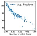
(a) ML-100K

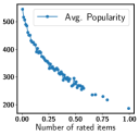
(b) ML-1M

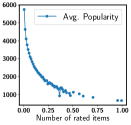
(c) ML-10M

(d) MT-200K

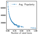
(e) Netflix

Figure 1: For each user $u$, we consider the set of items rated by $u$ in train $\mathcal{I}_{u}^{\mathcal{R}}$, and compute its average popularity $\bar{a}=\frac{1}{|\mathcal{I}_{u}^{\mathcal{R}}|}\sum_{i\in\mathcal{I}_{u}^{\mathcal{R}}}f_{i}^{\mathcal{R}}$. The x-axis shows the binned normalized $|\mathcal{I}_{u}^{\mathcal{R}}|$, while the y-axis plots the mean of the corresponding $\bar{a}$ values. The average popularity of items rated decreases as the number of items rated increases.

II-A Notation and data model

Let $\mathcal{U}$ denote the set of all consumers or users and $\mathcal{I}$ the set of all items. We reserve $u$, $s$ for indexing users, and $i$, $j$ for indexing items. Our dataset $\mathcal{D}$, is a set of ratings of users on various items, i.e., $\mathcal{D}=\{r_{ui}:u\in\mathcal{U},i\in\mathcal{I}\}$. Since every user rates only a small subset of items, $\mathcal{D}$ is a small subset of a complete rating matrix $\mathbf{R}$, i.e., $\mathcal{D}\subset\mathbf{R}\in\mathbb{R}^{|\mathcal{U}|\times|\mathcal{I}|}$.

We split $\mathcal{D}$ into a train set $\mathcal{R}$ and test set $\mathcal{T}$. Let $\mathcal{I}^{\mathcal{R}}$ ($\mathcal{I}^{\mathcal{T}}$) denote items in the train (test) set, with $\mathcal{I}_{u}^{\mathcal{R}}$ ($\mathcal{I}_{u}^{\mathcal{T}}$) denoting the items rated by a single user $u$ in the train (test) set. Let $\mathcal{U}_{i}^{\mathcal{R}}$ ($\mathcal{U}_{i}^{\mathcal{T}}$) denote users that rated item $i$ in the train (test) set. For each user, we generate a top-$N$ set by ranking all unseen train items, i.e., $\mathcal{I}^{\mathcal{R}}\setminus\mathcal{I}_{u}^{\mathcal{R}}$.

We denote the frequency of item $i$ in a given set $\mathcal{A}$ with $f_{i}^{\mathcal{A}}$. Following [14], the popularity of an item $i$ is its frequency in the train set, i.e., $f_{i}^{\mathcal{R}}=|\mathcal{U}_{i}^{\mathcal{R}}|$. Based on the Pareto principle [13], or the $80/20$ rule, we determine long-tail items, $\mathcal{L}$, as those that generate the lower $20\%$ of the total ratings in the train set, $\mathcal{L}\subset\mathcal{I}^{\mathcal{R}}$ (i.e, items are sorted in decreasing popularity). In our work, we use $x_{i}=\frac{x_{i}-\min(\mathbf{x})}{\max(\mathbf{x})-\min(\mathbf{x})}$ for normalizing a generic vector $\mathbf{x}$.

Table I summarizes our notation. We typeset the sets (e.g., $\mathcal{A}$), use upper case bold letters for matrices (e.g., $\mathbf{A}$), lower-case bold letters for vectors (e.g., $\mathbf{a}$), and lower case letters for scalar variables (e.g., $a$).

Parameter	Symbol
Dataset	$\mathcal{D}$
Train dataset	$\mathcal{R}$
Test dataset	$\mathcal{T}$
Set of users	$\mathcal{U}$
Set of items	$\mathcal{I}$
Set of long tail items in $\mathcal{R}$	$\mathcal{L}$
Specific user	$u$
Specific item	$i$
Set of items of $u$ in $\mathcal{R}$	$\mathcal{I}_{u}^{\mathcal{R}}$
Set of items of $u$ in $\mathcal{T}$	$\mathcal{I}_{u}^{\mathcal{T}}$
Set of users of $i$ in $\mathcal{R}$	$\mathcal{U}_{i}^{\mathcal{R}}$
Set of users of $i$ in $\mathcal{T}$	$\mathcal{U}_{i}^{\mathcal{T}}$
Rating of user $u$ on item $i$	$r_{ui}$
Size of top-$N$ set	$N$
Top-$N$ set of $u$	$\mathcal{P}_{u}$
Collection of top-$N$ sets for all users	$\mathcal{P}$
Long-tail novelty preference of user $u$ acc. model $m$	$\theta^{m}_{u}$
Accuracy function	$a(.)$
Coverage function	$c(.)$
Value function of user $u$	$v_{u}(.)$

TABLE I: Notation.

II-B Simple long-tail novelty preference models

Users have different preferences for discovering long-tail items. Given the train set $\mathcal{R}$, we need a measure of the user’s willingness to explore less popular items. Let $\theta_{u}^{m}$ denote user $u$’s preference for long-tail novelty as measured by model $m$.

Figure 1 plots the average popularity of rated items vs. the number of rated items (or user activity) for our datasets. As user activity increases, the average popularity of rated items decreases. This motivates an Activity measure $\theta_{u}^{A}=|\mathcal{I}_{u}^{\mathcal{R}}|$. But, most users only rate a few items, and $\theta_{u}^{A}$ does not indicate whether those items were long-tail or popular.

Instead, we can define a Normalized Long-tail measure

$$\small\theta_{u}^{N}=\frac{|\mathcal{I}_{u}^{\mathcal{R}}\cap\mathcal{L}|}{|\mathcal{I}_{u}^{\mathcal{R}}|}$$ (II.1)

which is the fraction of long-tail items in the user’s rated items. The higher this fraction, the higher her preference for long-tail items. However, $\theta_{u}^{N}$ does not capture the user’s interest (e.g, rating) in the items, and does not distinguish between the various long-tail items.

To resolve both problems, we can use similar notions as in TFIDF [25]. The rating an item receives from a particular user reflects its importance for that user. To capture the discriminative power of the item among the set of users and control for the fact that some items are generally more popular, we also incorporate an inverse popularity factor ($|\mathcal{U}_{i}^{\mathcal{R}}|$) that is logarithmically scaled. We define TFIDF-based measure using

$$\small\theta_{u}^{T}=\frac{1}{|\mathcal{I}_{u}^{\mathcal{R}}|}\sum_{i\in\mathcal{I}_{u}^{\mathcal{R}}}r_{ui}\log\left(\frac{|\mathcal{U}|}{|\mathcal{U}_{i}^{\mathcal{R}}|}\right)$$ (II.2)

This measure increases proportionally to the user rating $r_{ui}$, but is also counterbalanced by the popularity of the item. A higher $\theta_{u}^{T}$ shows more preference for less popular items. Although $\theta_{u}^{T}$ considers both the user interest $r_{ui}$, and the item popularity $|\mathcal{U}_{i}^{\mathcal{R}}|$, it has no indication about the preferences of the users in $\mathcal{U}_{i}^{\mathcal{R}}$. To address this limitation, observe Eq. II.2 can be re-written as

$$\small\theta_{u}^{T}=\frac{1}{|\mathcal{I}_{u}^{\mathcal{R}}|}\sum_{i\in\mathcal{I}_{u}^{\mathcal{R}}}\theta_{ui}=\frac{\sum_{i\in\mathcal{I}_{u}}w_{i}\theta_{ui}}{\sum_{i\in\mathcal{I}_{u}}w_{i}}$$ (II.3)

where $\theta_{ui}=r_{ui}\log\left(\frac{|\mathcal{U}|}{|\mathcal{U}_{i}^{\mathcal{R}}|}\right)$ is a per-user-item long-tail preference value, and $w_{i}=1$ for all items. Basically, $\theta_{u}^{T}$ gives equal importance to all items and is a crude average of $\theta_{ui}$.

We can generalize the idea in Eq. II.3. Specifically, for each user, we consider a generalized long-tail novelty preference estimate, $\theta_{u}^{G}$. We assume $\theta_{u}^{G}$ is a weighted average of $\theta_{ui}$. However, rather than imposing equal weights, we define $w_{i}$ to indicate an item importance weight. Our second assumption is that an item is important when its users do not regard it as a mediocre item; when their preference for that item deviates from their generalized preference. In other words, an item $i$ is important when $\sum_{u\in\mathcal{U}_{i}^{\mathcal{R}}}(\theta_{ui}-\theta_{u}^{G})^{2}$ is large. Since $w_{i}$ and $\theta^{G}_{u}$ influence each other, below we describe how to learn these variables in a joint optimization objective.

II-C Learning generalized long-tail novelty preference

We define $\epsilon_{i}=\big{[}\sum_{u\in\mathcal{U}_{i}^{\mathcal{R}}}1-\big{(}\theta_{ui}-\theta_{u}^{G}\big{)}^{2}\big{]}$ as the item mediocrity coefficient. Assuming $|\theta_{ui}-\theta_{u}^{G}|\leq 1$ (explained later), the maximum of $\epsilon_{i}$ is obtained when $\theta_{ui}=\theta_{u}^{G}$. We formulate our objective as:

$$\ O(\mathbf{w},\bm{\theta}^{G})=\sum_{i\in\mathcal{I}^{\mathcal{R}}}w_{i}\big{[}\sum_{u\in\mathcal{U}_{i}^{\mathcal{R}}}1-\big{(}\theta_{ui}-\theta_{u}^{G}\big{)}^{2}\big{]}=\sum_{i\in\mathcal{I}^{\mathcal{R}}}w_{i}\epsilon_{i}$$

which is the total weighted mediocrity. Here, $\mathcal{I}^{\mathcal{R}}$ are the items in train, $\mathcal{U}_{i}^{\mathcal{R}}$ denotes users that rated item $i$ in the train set (Section II-A), and $\theta_{ui}$ is the per-user-item preference value, computed from rating data. Our objective has two unknown variables: $\bm{\theta}^{G}\in\mathbb{R}^{|\mathcal{U}|}$, $\mathbf{w}\in\mathbb{R}^{|\mathcal{I}|}$. We use an alternating optimization approach for optimizing $\mathbf{w}$ and $\bm{\theta}^{G}$. When optimizing w.r.t. $\mathbf{w}$, we must minimize the objective function in accordance with our intuition about $w_{i}$. In particular, for larger mediocrity coefficient, we need smaller weights. On the other hand, when optimizing w.r.t. $\bm{\theta}^{G}$, we need to increase the closeness between $\theta_{u}^{G}$ and all $\theta_{ui}$’s, which is aligned with our intuition about $\theta_{u}^{G}$. So, we have to maximize the objective function w.r.t. $\bm{\theta}^{G}$. Our final objective is a minimax problem:

$$\min_{\mathbf{w}}\max_{\bm{\theta}^{G}} O(\mathbf{w},\bm{\theta}^{G})-\lambda_{1}\sum_{i\in\mathcal{I}^{\mathcal{R}}}\log{w_{i}}$$ (II.4)

where we have added a regularizor term $\sum_{i\in\mathcal{I}^{\mathcal{R}}}\log{w_{i}}$ to prevent $w_{i}$ from approaching 0 [26].

When $\bm{\theta}^{G}$ is fixed, we need to solve a minimization problem involving only $\mathbf{w}$. By taking the derivative w.r.t. $w_{i}$ we have

$$w_{i}=\frac{\lambda_{1}}{\sum_{u\in\mathcal{U}_{i}^{\mathcal{R}}}1-\big{(}\theta_{ui}-\theta_{u}^{G}\big{)}^{2}}=\frac{\lambda_{1}}{\epsilon_{i}}$$ (II.5)

When $\mathbf{w}$ is fixed, we need to solve a maximization problem involving $\bm{\theta}^{G}$. Taking the derivative w.r.t. $\theta_{u}^{G}$ we derive

$$\theta_{u}^{G}=\frac{\sum_{i\in\mathcal{I}_{u}^{\mathcal{R}}}w_{i}\theta_{ui}}{\sum_{i\in\mathcal{I}_{u}^{\mathcal{R}}}w_{i}}$$ (II.6)

Essentially, Eq. II.5 characterizes an item’s weight, based on the item mediocrity. The higher the mediocrity, the lower the weight. Moreover, for every user $u$, $\theta_{u}^{G}$ is a weighted average of all $\theta_{ui}$. Note, in Eq. II.6, $\theta_{u}^{G}=\theta_{u}^{T}$ when $w_{i}=1$ for all items. Our generalized $\theta_{u}^{G}$ incorporates both the user interest and popularity of items (via $\theta_{ui}$), and the preferences of other users of the item (via $w_{i}$). Furthermore, since we need $|\theta_{ui}-\theta_{u}^{G}|\leq 1$, and prefer $\theta_{u}^{G}\in[0,1]$, we project all $\theta_{ui}$ to the $[0,1]$ interval before applying the algorithm. We also set $\lambda_{1}=1$.

III GANC: Generic Re-ranking Framework

We define user satisfaction based on the accuracy of the top-$N$ set and its coverage of the item space, so as to introduce novelty and serendipity into recommendation sets. We consider three components for our framework: 1. an accuracy recommender (ARec) that is responsible for suggesting accurate top-$N$ sets. 2. a coverage recommender (CRec) that is responsible for suggesting top-$N$ sets that maximize coverage across the item space, and consequently promote long-tail items. 3. the user preference for long-tail novelty $\theta_{u}\in[0,1]$. We use the template $\texttt{GANC}(\texttt{ARec},\bm{\theta},\texttt{CRec)}$ to specify the used components.

We define individual user value functions for a top-$N$ set $\mathcal{P}_{u}$ as

$$\small v_{u}(\mathcal{P}_{u})=(1-\theta_{u})a(\mathcal{P}_{u})+\theta_{u}c(\mathcal{P}_{u})$$ (III.1)

where $a(.)$ measures the score of a set of items according to the accuracy recommender, and $c(.)$ measures the score of a set according to the coverage recommender. With slight abuse of notation, let $a(i)$ and $c(i)$ denote the accuracy score and coverage score of a single item $i$. We ensure $a(i),c(i)\in[0,1]$ to have the same scale. Furthermore, we define $a(\mathcal{P}_{u})=\sum_{i\in\mathcal{P}_{u}}a(i)$ and $c(\mathcal{P}_{u})=\sum_{i\in\mathcal{P}_{u}}c(i)$.

The user value function in Eq. III.1 positively rewards sets that increase coverage. Similar intuitions for encouraging solutions with desirable properties, e.g., diverse solutions, have been used in related work [27]. However, their trade-off parameters are typically obtained via parameter tuning or cross validation. By contrast, we impose personalization via the user preference estimate, $\theta_{u}$, that is learned based on historical rating data. Next, we list the various base recommender models integrated into GANC.

III-A Accuracy recommender

The accuracy recommender provides an accuracy score, $a(i)$, for each item $i$. We experiment with three models (Section IV-A provides details and setup configurations):

• Most popular (Pop)  [1] is non-personalized and recommends the most popular unseen items. It makes accurate recommendations, but has low coverage and novelty [1]. Since it does not score items, we define $a(i)=1$ if item $i$ is in the top-$N$ set suggested by Pop, otherwise $a(i)=0$.

• Regularized SVD (RSVD) [28] learns latent factors for users and items by analyzing user-item interaction data (e.g., ratings). The factors are then used to predict the values of unobserved ratings. We use RSVD to compute a predicted rating matrix $\mathbf{\hat{R}}\in\mathbb{R}^{|\mathcal{U}|\times|\mathcal{I}|}$. We normalize the predicted rating vectors of all users to ensure $\hat{r}_{ui}\in[0,1]$, and define $a(i)=\hat{r}_{ui}$.

• PureSVD (PSVD) [1] is also a latent factor model. We follow the same procedure as RSVD, using PSVD factors [1]. Note, PSVD scores correspond to associations between users and items.

III-B Coverage recommender

The coverage recommender provides a coverage score, $c(i)$, for each item $i$. We use three coverage recommenders:

• Random (Rand) recommends $N$ unseen items randomly. It has high coverage, but low accuracy [5]. We define $c(i)\sim$unif$(0,1)$.

• Static (Stat) focuses exclusively on promoting less popular items. We define $c(i)$ to be a monotone decreasing function of $f_{i}^{\mathcal{R}}$, the popularity of $i$ in the train set $\mathcal{R}$. We use $c(i)=\frac{1}{\sqrt{f_{i}^{\mathcal{R}}+1}}$ in our work. Note the gain of recommending an item is constant.

• Dynamic (Dyn) allows us to better correct for the popularity bias in recommendations. In particular, rather than the train set $\mathcal{R}$, we define $c(i)$ based on the set of recommendations made so far. Let $\mathcal{P}=\{\mathcal{P}_{u}\}_{u=1}^{|\mathcal{U}|}$ with $|\mathcal{P}_{u}|=N$, denote the collection of top-$N$ sets assigned to all users, and $\mathcal{A}=\{\mathcal{A}_{u}\}_{u=1}^{|\mathcal{U}|}$ with $\mathcal{A}_{u}\subseteq\mathcal{P}_{u}$, denote a partial collection where a subset of users have been assigned some items. We measure the long-tail appeal of an item using a monotonically decreasing function of the popularity of $i$ in $\mathcal{A}$, i.e., $f_{i}^{\mathcal{A}}$. We use $c(i)=\frac{1}{\sqrt{f_{i}^{\mathcal{A}}+1}}$ in our work. The main intuition is that recommending an item has a diminishing returns property: the more the item is recommended, the less the gain of the item in coverage, i.e., $c(i)=1$ when $\mathcal{A}=\emptyset$, but decreases as the item is more frequently suggested.

III-C Optimization Algorithm for GANC

The overall goal of the framework is to find an optimal top-$N$ collection $\mathcal{P}=\{\mathcal{P}_{u}\}_{u=1}^{|\mathcal{U}|}$ that maximizes the aggregate of the user value functions:

$$\small\max_{\mathcal{P}}\ v(\mathcal{P})=\sum_{u\in\mathcal{U}}v_{u}(\mathcal{P}_{u})$$ (III.2)

The combination of Rand and Stat with the accuracy recommenders in Section III-A, result in value functions that can be optimized greedily and independently, for each user. Using Dyn, however, creates a dependency between the optimization of user value functions, where the items suggested to one user depend on those suggested to previous users. Therefore, user value functions can no longer be optimized independently.

Input: $N,S,\mathcal{U},\mathcal{I},\mathcal{R}$

Output: $\mathcal{P}$

1 $\mathbf{f}\leftarrow 0,\mathcal{P}\leftarrow\emptyset,\bm{\theta}\leftarrow$ Estimate from $\mathcal{R}$ (Section II);

2 $\mathcal{S}\leftarrow$ Sample $S$ users from $\mathcal{U}$ acc. to KDE($\bm{\theta}$);

3 Sort $\mathcal{S}$ in increasing $\bm{\theta}$;

// Performed sequentially for users in sample

4 foreach $u\in\mathcal{S}$ do

5       Update Dyn function parameter $\mathbf{f}$;

6       $\mathcal{P}_{u}$ = $\mathcal{P}_{u}$ $\cup$ $\operatorname*{argmax}_{i\in\mathcal{I}}$ $v_{u}(\mathcal{P}_{u}\cup i)$ - $v_{u}(\mathcal{P}_{u})$;

7      

8      foreach $i\in\mathcal{P}_{u}$ do $\mathbf{f}_{i}=\mathbf{f}_{i}+1$;

9       F($\theta_{u}$) $\leftarrow\mathbf{f}$;

10       $\mathcal{P}=\mathcal{P}\cup\mathcal{P}_{u}$;

11      

12 end foreach

// Performed in parallel for users not in sample

13 foreach $u\in\mathcal{U}\setminus\mathcal{S}$ do

14       $\mathbf{\hat{f}}\leftarrow F(\operatorname*{argmin}(\theta_{s}-\theta_{u}))$ for $s\in\mathcal{S}$;

15       Update Dyn function parameter $\mathbf{\hat{f}}$;

16       $\mathcal{P}_{u}$ = $\mathcal{P}_{u}$ $\cup$ $\operatorname*{argmax}_{i\in\mathcal{I}}$ $v_{u}(\mathcal{P}_{u}\cup i)$ - $v_{u}$ $\mathcal{P}=\mathcal{P}\cup\mathcal{P}_{u}$;

17      

18 end foreach

return $\mathcal{P}$

Algorithm 1 GANC with OSLG optimization

Optimization algorithm for GANC with Dyn. Because Dyn is monotonically decreasing in $f_{i}^{\mathcal{A}}$, when used in Eq.III.1, the overall objective in Eq. III.2 becomes submodular across users. Maximizing a submodular function is NP-hard [29]. However, a key observation is that the constraint of recommending $N$ items to each user, corresponds to a partition matroid over the users. Finding a top-$N$ collection $\mathcal{P}$ that maximizes Eq. III.2 is therefore an instance of maximizing a submodular function subject to a matroid constraint (see Appendix -B). A Locally Greedy heuristic, due to Fisher et al. [30], can be applied: consider the users separately and in arbitrary order. At each step, select a user $u$ arbitrarily, and greedily construct $\mathcal{P}_{u}$ for that user. Proceed until all users have been assigned top-$N$ sets. Locally Greedy produces a solution at least half the optimal value for maximizing a submodular monotone function subject to a matroid constraint [30].

However, locally greedy is sequential and has a computational complexity of $O(|\mathcal{U}|.|\mathcal{I}|.N)$ which is not scalable. Instead, we introduce a heuristic we call Ordered Sampling-based Locally Greedy (OSLG). Essentially, we make two modifications based on the user long-tail preferences: first, proportionate to the distribution of user long-tail preferences $\bm{\theta}$, we sample a subset of users, and run the sequential algorithm on this sample only. Second, to allow the system to recommend more established or popular products to users with lower long-tail preference, instead of arbitrary order, we modify locally greedy to consider users in increasing long-tail preference.

Algorithm 1 shows GANC with OSLG optimization: We use $\mathbf{f}_{i}$ as a shorthand for $f_{i}^{\mathcal{A}}$, the popularity of item $i$ in the current set of recommendations, used in Dyn. First, $\mathbf{f}$ is initialized and user preferences $\bm{\theta}$ are estimated (line 1). Next, we use Kernel density estimation (KDE) [31] to approximate the Probability density function (PDF) of $\bm{\theta}$, and use the PDF to draw a sample $\mathcal{S}$ of size $S$ from $\bm{\theta}$ and find the corresponding users in $\mathcal{U}$ (line 1). The sampled users are then sorted in increasing long-tail preference (line 1), and the algorithm iterates over the users. In each iteration, it updates the Dyn function (line 1) and assigns a top-$N$ set to the current user by maximizing her value function (line 1). The Dyn function parameter $\mathbf{f}$ is then updated w.r.t. the recently assigned top-$N$ set (line 1). Moreover, $\mathbf{f}$ is associated with the current long-tail preference estimate $\theta_{u}$, and stored (line 1). The algorithm then proceeds to the next user. Since Dyn is monotonically decreasing in $\mathbf{f}_{i}$, frequently recommended items are weighted down by the value function of subsequent users. Consequently, as we reach users who prefer long-tail items and discovery, their value functions prefer relatively unpopular items that have not been recommended before. Thus, the induced user ordering, results in the promotion of long-tail items to the right group of users, such that we obtain better coverage while maintaining user satisfaction.

For each user not included in the sample set, $u\not\in\mathcal{S}$, we find the most similar user $s\in\mathcal{S}$, where similarity is defined as $|\theta_{s}-\theta_{u}|$ (line 1), and use $F(\theta_{s})$ to compute the coverage score (line 1), and assign a top-$N$ set. Observe, the value functions of $u\in\mathcal{U}\setminus\mathcal{S}$, are independent of each other, and lines 1-1 can be performed in parallel. The computational complexity of the sequential part drops to $O(|\mathcal{S}|.|\mathcal{I}|.N)$ at the cost of $O(|\mathcal{S}|.|\mathcal{I}|)$ extra memory.

IV Empirical Evaluation

IV-A Experimental setup

Datasets and data split. Table II describes our datasets. We use MovieLens 100K (ML-100K), 1 Million (Ml-1M), 10 Million (ML-10M) ratings [32], Netflix, and MovieTweetings 200K (MT-200K) [33]. In the MovieLens datasets, every consumer has rated at least 20 movies ($\tau=20$), with $r_{ui}\in\{1,\dots,5\}$ (ML-10M has half-star increments). MT-200K contains voluntary movie ratings posted on twitter, with $r_{ui}\in\{0,\dots,10\}$. Following [34], we preprocessed this dataset to map the ratings to the interval $[1,5]$. Due to the extreme sparsity of this dataset and to ensure every user has some data to learn from, we filtered the users to keep those with at least 5 ratings ($\tau=5$).

Our selected datasets have varying density levels. Additionally, MT-200K and Netflix include a large number of difficult infrequent users, i.e., in MT-200K, 47.42% (3.37% in Netflix) of the users have rated fewer than 10 items, with the minimum being 4. We chose these datasets to study performance in settings where users provide few feedback [4, 21].

Next, we randomly split each dataset into train and test sets by keeping a fixed ratio $\kappa$ of each user’s ratings in the train set and moving the rest to the test set [35]. This way, when $\kappa=0.8$, an infrequent user with 5 ratings will have 4 train and 1 test rating, while a user with 100 ratings, will have 80 train ratings and the rest in test. For ML-1M and ML-10M, we set $\kappa=0.5$. For MT-200K, we set $\kappa=0.8$. For Netflix, we use their probe set as our test set, and remove the corresponding ratings from train. We remove users in the probe set who do not appear in train set, and vice versa.

Dataset	$|\mathcal{D}|$	$|\mathcal{U}|$	$|\mathcal{I}|$	d$\%$	$\mathcal{L}\%$	$\kappa$	$\tau$
ML-100K	100K	943	1682	6.30	66.98	0.5	20
ML-1M	1M	6,040	3,706	4.47	67.58	0.5	20
ML-10M	10M	69,878	10,677	1.34	84.31	0.5	20
MT-200k	172,506	7,969	13,864	0.16	86.84	0.8	5
Netflix	98,754,394	459,497	17,770	1.21	88.27	-	-

TABLE II: Datasets description. $|\mathcal{D}|$ is number of ratings in dataset. Density is $\text{d}\%=|\mathcal{D}|/(|\mathcal{U}|*|\mathcal{I}|)\times 100\%$. Long-tail percentage is $\mathcal{L}\%=(|\mathcal{L}|/|\mathcal{I}^{\mathcal{R}}|)\times 100\%$. Train-test split ratio per user is $\kappa$, $\tau$ is the minimum number of ratings per user.

Local Ranking Accuracy Metrics	$\mathrm{Precision@N}=\frac{1}{N|\mathcal{U}|}\sum_{u\in\mathcal{U}}|\mathcal{I}_{u}^{\mathcal{T}+}\cap\mathcal{P}_{u}|$
	$\mathrm{Recall@N}=\frac{1}{|\mathcal{U}|}\sum_{u\in\mathcal{U}}\frac{|\mathcal{I}_{u}^{\mathcal{T}+}\cap\mathcal{P}_{u}|}{|\mathcal{I}_{u}^{\mathcal{T}+}|}$
	$\mathrm{F}\textnormal{-}\mathrm{measure@N}=\frac{\mathrm{Precision@N}.\mathrm{Recall@N}}{\mathrm{Precision@N}+\mathrm{Recall@N}}$
Longtail Promotion	$\mathrm{LTAccuracy@N}=\frac{1}{N|\mathcal{U}|}\sum_{u\in\mathcal{U}}|\mathcal{L}\cap\mathcal{P}_{u}|$
	$\mathrm{StratRecall@N}=\frac{\sum_{u\in\mathcal{U}}\sum_{i\in\mathcal{I}_{u}^{\mathcal{T}+}\cap\mathcal{P}_{u}}\big{(}\frac{1}{f_{i}^{\mathcal{R}}}\big{)}^{\beta}}{{\sum_{u\in\mathcal{U}}\sum_{i\in\mathcal{I}_{u}^{\mathcal{T}+}}\big{(}\frac{1}{f_{i}^{\mathcal{R}}}\big{)}^{\beta}}}$
Coverage Metrics	$\mathrm{Coverage@N}=\frac{|\cup_{u\in\mathcal{U}}\mathcal{P}_{u}|}{|\mathcal{I}|}$
	$\mathrm{Gini@N}=\frac{1}{|\mathcal{I}|}(|\mathcal{I}|+1-2\frac{\sum_{j=1}^{|\mathcal{I}|}(|\mathcal{I}|+1-j)f[j]}{\sum_{j=1}^{|\mathcal{I}|}f[j]})$

TABLE III: Performance Metrics. Notation is in Section II-A. For gini, the vector $\mathbf{f}$ is sorted in non-decreasing order of recommendation frequency of items, i.e., $f[j]\leq f[j+1]$.

Test ranking protocol and performance metrics. For testing, we adopt the “All unrated items test ranking protocol” [36, 5] where for each user, we generate the top-$N$ set by ranking all items that do not appear in the train set of that user (details in Appendix -C).

Table III summarizes the performance metrics. To measure how accurately an algorithm can rank items for each user, we use local rank-based precision and recall [37, 5, 36], where each metric is computed per user and then averaged across all users. Precision is the proportion of relevant test items in the top-$N$ set, and recall is the proportion of relevant test items retrieved from among a user’s relevant test items. As commonly done in the literature [37, 38], for each user $u$, we define her relevant test items as those that she rated highly, i.e., $\mathcal{I}_{u}^{\mathcal{T}+}=\{i:i\in\mathcal{I}_{u}^{\mathcal{T}},r_{ui}\geq 4\}$. Note, because the collected datasets have many missing ratings, the hypothesis that only the observed test ratings are relevant, underestimates the true precision and recall [36]. But, this holds for all algorithms, and the measurements are known to reflect performance in real-world settings [36]. F-measure is the harmonic mean of precision and recall.

We use Long-Tail Accuracy (LTAccuracy@$N$) [20] to measure the novelty of recommendation lists. It computes the proportion of the recommended items that are unlikely to be seen by the user. Moreover, we use Stratified Recall (StratRecall@$N$) [36] which measures the ability of a model to compensate for the popularity bias of items w.r.t train set. Similar to [36], we set $\beta=0.5$. Note, LTAccuracy emphasizes a combination of novelty and coverage, while Stratified Recall emphasizes a combination of novelty and accuracy.

For coverage we use two metrics: Coverage@$N$ is the ratio of the total number of distinct recommended items to the total number of items [20, 5]. A maximum value of $1$ indicates each item in $\mathcal{I}$ has been recommended at least once. Gini [39], measures the inequality among values of a frequency distribution $\mathbf{f}$. It lies in $[0,1]$, with $0$ representing perfect equality, and larger values representing skewed distributions. In Table III, $\mathbf{f}$ is the recommendation frequency of items, and is sorted in non-decreasing order, i.e., $f[j]\leq f[j+1]$.

Other algorithms and their configuration. We compare against, or integrate the following methods in our framework .

• Rand is non-personalized and randomly suggests $N$ unseen items from among all items. It obtains high coverage and novelty, but low accuracy [5].

• Pop [1] is a non-personalized algorithm. For ranking tasks, it obtains high accuracy [1, 5], since it takes advantage of the popularity bias of the data. However, Pop makes trivial recommendations that lack novelty [1].

• RSVD [40] is a latent-factor model for rating prediction. We used LIBMF, with L2-Norm as the loss function, and L2-regularization, and Stochastic Gradient Descent (SGD) for optimization. We also tested the same model with non-negative constraints (RSVDN) [28], but did not find significant performance difference. We omit RSVDN from our results. We performed 10-fold cross validation and tested: number of latent factors $g\in\{8,20,40,50,80,100\}$, L2-regularization coefficients $\lambda\in\{0.001,0.005,0.01,0.05,0.1\}$, learning rate $\eta\in\{0.002,0.003,0.01,0.03\}$. For each dataset, we used the parameters that led to best performance (see Appendix -A).

• PSVD [1] is a latent factor model, known for achieving high accuracy and novelty [1]. In PSVD, missing values are imputed by zeros and conventional SVD is performed. We used Python’s sparsesvd module and tested number of latent factors $g\in\{10,20,40,60,100,150,200,300\}$. We report results for two configurations: one with $10$ latent factors (PSVD10), and one with 100 latent factors (PSVD100).

• CoFiRank [41] is a ranking prediction model that can optimize directly the Normalized Discounted Cumulative Gain (NDCG) ranking measure [42]. We used the source code from [41], with parameters set according to [41]: 100 dimensions and $\lambda=10$, and default values for other parameters. We experimented with both regression (squared) loss (CofiR100) and NDCG loss (CofiN100). Similar to [43, 44], we found CofiR100 to perform consistently better than CofiN100 in our experiments on ML-1M and ML-100K. We only report results for CofiR100.

• Ranking-Based Techniques (RBT) [14] maximize coverage by re-ranking the output of a rating prediction model according to a re-ranking criterion. We implemented two variants: one that re-ranks a few of the items in the head according to their popularity (Pop criterion), and another which re-ranks according to the average rating (Avg criterion). As in [14], we set $T_{max}=5$ in all datasets. The parameter $T_{R}$ controls the extent of re-ranking. We tested $T_{R}\in[4,4.2,4.5]$, and found $T_{R}=4.5$ to yield more accurate results. Furthermore, because our datasets contain a wider range of users compared to [14], we set $T_{H}=1$ on all datasets, except ML-10M and Netflix, where we set $T_{H}=0$. To refer to RBT variants, we use $\texttt{RBT}(\texttt{ARec},\texttt{Re-ranking criterion})$.

• Resource allocation [20] is an method for re-ranking the output of a rating prediction model. It has two phases: 1. resources are allocated to items according to the received ratings, and 2. the resources are distributed according to the relative preferences of the users, and top-$N$ sets are generated by assigning a a 5D score (for accuracy, balance, coverage, quality, and quantity of long-tail items) to every user-item pair. We use the variants proposed in [20], which are combinations of the scoring function (5D) with the rank by rankings (RR) and accuracy filtering (A) algorithms (Section 3.2.2 in [20]). We use the template $\texttt{5D}(\texttt{ARec},\texttt{A},\texttt{RR})$ to show the different combinations, where A and RR are optional. We implemented and ran all four variants with default values set according to [20]: $k=3.|\mathcal{I}|$ and $q=1$.

• Personalized Ranking Adaptation (PRA) [22] is a generic re-ranking framework, that first estimates user tendency for various criteria like diversity and novelty, then iteratively and greedily re-ranks items in the head of the recommendations to match the top-$N$ set with the user tendencies. We compare with the novelty-based variant of this framework, which relies on item popularity statistics to measure user novelty tendencies. We use the the mean-and-deviation based heuristic, that is measured using the popularity of rated items, and was shown to provide comparable results with other heuristics in [22]. For the configurable parameters, we followed [22]: Sample set size $S_{u}\in\min(|\mathcal{I}^{\mathcal{R}}_{u}|,10)$, the exchangeable set size $|X_{u}|\in\{10,20\}$, and used “optimal swap” strategy with $maxSteps=20$. We use the template $\texttt{PRA}(\texttt{ARec},|X_{u}|)$ to refer to variants of PRA.

IV-B Distribution of long-tail novelty preferences

Figure 2 plots the histogram of various long-tail preference models. We observe $\theta^{A}_{u}$ is skewed to the right. This is due to the sparsity problem, where the majority of users rate a few items. $\theta^{N}_{u}$ is also skewed to the right across all datasets, due to both the popularity bias and sparsity problems [37, 45]. On the other hand, $\theta^{G}_{u}$ is normally distributed, with a larger mean and a larger variance, on all datasets. In the experiments in Section IV-C, we study the effect of these preference models on performance.

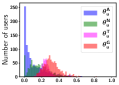
(a) ML-100K

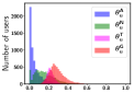
(b) ML-1M

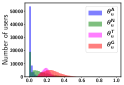
(c) ML-10M

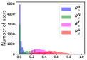
(d) MT-200K

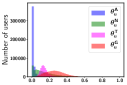
(e) Netflix

Figure 2: Histogram of long-tail novelty preference models. Observe $\theta^{A}_{u}$ is skewed toward smaller values because of sparsity, i.e., the majority of users rate a few items. $\theta^{N}_{u}$ is also biased toward smaller values, due to a combination of popularity bias and sparsity. $\theta^{T}_{u}$ and $\theta^{G}_{u}$ are less biased and more normally distributed and alleviate both problems.

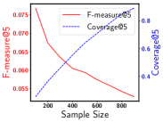
(a) PSVD100

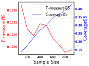
(b) PSVD10

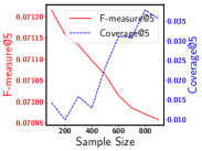
(c) Pop

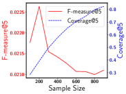
(d) RSVD

Figure 3: Performance of GANC(ARec, $\bm{\theta}^{G}$, Dyn) with OSLG optimization, as sample size (S) is varied. The accuracy recommender ARec is indicated in each sub-figure. Dataset is ML-1M.

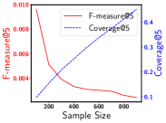
(a) PSVD100

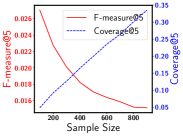
(b) PSVD10

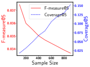
(c) Pop

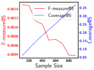
(d) RSVD

Figure 4: Performance of GANC(ARec, $\bm{\theta}^{G}$, Dyn) with OSLG optimization, as sample size (S) is varied. The accuracy recommender ARec is indicated in each sub-figure. Dataset is MT-200K.

IV-C Performance of GANC with Dyn coverage recommender

When Dyn is integrated in GANC, we use OSLG optimization. We run variants of GANC that involve randomness (e.g., sampling-based variants) 10 times and report the average.

Effect of sample size. The sample size $S$ is a system-wide hyper-parameter in the OSLG algorithm, and should be determined w.r.t. preference for accuracy or coverage, and the accuracy recommender. For tuning $S$, we run experiments on ML-1M, and assess its effect on F-measure and coverage. As shown in Figures 3 and 4, increasing $S$, increases coverage and decreases the F-measure of most accuracy recommenders. Regarding RSVD, the scores output by this model lead to the initial decrease and later increase of F-measure. Since we want to maintain accuracy, we fix $S=500$ in the rest of our experiments, although a larger $S$ can be used.

Effect of the user long-tail novelty preference model, the accuracy recommender, and their interplay. We evaluate GANC with Dyn coverage, i.e., GANC(ARec, $\bm{\theta}$, Dyn), while varying the accuracy recommender ARec, and the long-tail novelty preference model $\bm{\theta}$. We examine the following long-tail preference models:

• Random $\bm{\theta}^{R}$ randomly initializes $\theta^{R}_{u}$ (10 times per user).

• Constant $\bm{\theta}^{C}$ assigns the same constant value $C$ to all users. We report results for $C=0.5$.

• Normalized Long-tail $\bm{\theta}^{N}$ (Eq. II.1) measures the proportion of long-tail items the user has rated in the past.

• Tfidf-based $\bm{\theta}^{T}$ (Eq. II.2) incorporates user interest and popularity of items.

• Generalized $\bm{\theta}^{G}$ (Eq. II.6) incorporates user interest, popularity of items, and the preferences of other users.

Due to sampling ($S=500$), we run each variant 10 times (with random shuffling for $\bm{\theta}^{C}$) and average over the runs. We run the experiments on ML-1M.

Figure 5d shows performance of GANC(ARec, $\bm{\theta}$, Dyn) as $\bm{\theta}$ and the accuracy recommender (ARec) are varied. Across all rows, as expected, the accuracy recommender on its own, typically obtains the best F-measure. Moreover, $\bm{\theta}^{R}$ and $\bm{\theta}^{C}$ often have the lowest F-measure. Different variants of GANC with $\bm{\theta}^{N},\bm{\theta}^{T}$, and $\bm{\theta}^{G}$ are generally in the middle, which shows that these preference estimates are better than $\bm{\theta}^{R}$ and $\bm{\theta}^{C}$ in terms of accuracy. For Stratified Recall, similar trends as accuracy are observed in the ranking of the algorithms. The trends are approximately the same as we vary the accuracy recommender in Figures 5d.b, 5d.c, and 5d.d.

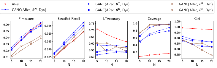
(a) Accuracy recommender (ARec) is RSVD

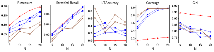
(b) Accuracy recommender (ARec) is PSVD100

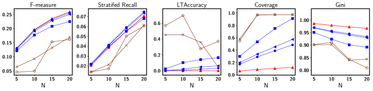
(c) Accuracy recommender (ARec) is PSVD10

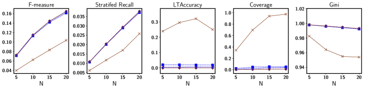
(d) Accuracy recommender (ARec) is Pop

Figure 5: Performance of GANC(ARec, $\bm{\theta}$, Dyn), with fixed sample size $S=|500|$, different accuracy recommenders (ARec), and different long-tail preference models ($\bm{\theta}$). Dataset is ML-1M. The trends are approximately the same as we vary the accuracy recommender in Figures 5d.a, 5d.b, 5d.c, and 5d.d. In each row, ARec typically achieves the highest F-measure, but performs poorly w.r.t. coverage and gini. Variants of our framework that use $\bm{\theta}^{G}$, $\bm{\theta}^{T}$, $\bm{\theta}^{N}$, obtain higher f-measure levels compared to those that use $\bm{\theta}^{R}$ and $\bm{\theta}^{C}$. They also improve stratified recall, independent of the accuracy recommender. Stratified Recall emphasizes novelty and accuracy

.

V Comparison with other recommendation models

We conduct two rounds of experiments: first, we evaluate re-ranking frameworks that post-process rating-prediction models, then we study general top-$N$ recommendation algorithms. For GANC, we run variants that involve randomness (e.g., sampling-based variants) 10 times, and report the average.

V-A Comparison with re-ranking methods for rating-prediction

Standard re-ranking frameworks typically use a rating prediction model as their accuracy recommender. In this section, we use RSVD as the underlying rating prediction model, and analyze performance across datasets with varying density levels. We compared the standard greedy ranking strategy of RSVD with 5D(RSVD), 5D(RSVD, A, RR), RBT(RSVD, Pop), RBT(RSVD, Avg), PRA(RSVD,10), PRA(RSVD,20), GANC(RSVD, $\bm{\theta}^{T}$, Dyn), and GANC(RSVD, $\bm{\theta}^{G}$, Dyn). We report results for $N=5$, since users rarely look past the items at the top of recommendation sets. Table V-A shows top-$5$ recommendation performance.

	Alg.	F@5	S@5	L@5	C@5	G@5	Score
ML-100K	RSVD	0.0279 (2)	0.0098 (4)	0.6649 (4)	0.0707 (8)	0.9886 (9)	5.4 (4)
	5D(RSVD)	0.0013 (9)	0.0014 (9)	0.9260 (1)	0.2586 (3)	0.9000 (3)	5.0 (2)
	5D(RSVD, A, RR)	0.0071 (8)	0.0035 (8)	0.7669 (2)	0.1171 (7)	0.9783 (8)	6.6 (6)
	RBT(RSVD, Pop)	0.0136 (7)	0.0043 (7)	0.7362 (3)	0.1284 (6)	0.9759 (7)	6.0 (5)
	RBT(RSVD, Avg)	0.0201 (6)	0.0075 (6)	0.6271 (5)	0.1938 (4)	0.9583 (5)	5.2 (3)
	PRA(RSVD, 10)	0.0252 (5)	0.0103 (3)	0.5642 (6)	0.1171 (7)	0.9674 (6)	5.4 (4)
	PRA(RSVD, 20)	0.0255 (4)	0.0095 (5)	0.5544 (7)	0.1379 (5)	0.9581 (4)	5.0 (2)
	GANC(RSVD, $\bm{\theta}^{T}$, Dyn)	0.0310 (1)	0.0127 (1)	0.5064 (9)	0.6260 (2)	0.7669 (2)	3.0 (1)
	GANC(RSVD, $\bm{\theta}^{G}$, Dyn)	0.0260 (3)	0.0122 (2)	0.5501 (8)	0.8716 (1)	0.6242 (1)	3.0 (1)

ML-1M RSVD 0.0208 (3) 0.0050 (6) 0.7091 (3) 0.0758 (9) 0.9923 (9) 6.0 (6) 5D(RSVD) 0.0008 (9) 0.0006 (9) 0.9579 (1) 0.1927 (4) 0.9468 (3) 5.2 (4) 5D(RSVD, A, RR) 0.0167 (6) 0.0052 (5) 0.6649 (5) 0.1360 (6) 0.9752 (6) 5.6 (5) RBT(RSVD, Pop) 0.0091 (8) 0.0022 (8) 0.8019 (2) 0.1125 (8) 0.9872 (8) 6.8 (7) RBT(RSVD, Avg) 0.0155 (7) 0.0044 (7) 0.6816 (4) 0.2261 (3) 0.9704 (4) 5.0 (3) PRA(RSVD, 10) 0.0207 (4) 0.0053 (4) 0.6268 (6) 0.1171 (7) 0.9800 (7) 5.6 (5) PRA(RSVD, 20) 0.0205 (5) 0.0055 (3) 0.5976 (7) 0.1436 (5) 0.9714 (5) 5.0 (3) GANC(RSVD, $\bm{\theta}^{T}$, Dyn) 0.0244 (1) 0.0077 (1) 0.5139 (9) 0.5113 (2) 0.8947 (2) 3.0 (2) GANC(RSVD, $\bm{\theta}^{G}$, Dyn) 0.0213 (2) 0.0072 (2) 0.5355 (8) 0.6492 (1) 0.8754 (1) 2.8 (1) ML-10M RSVD 0.0147 (1) 0.0021 (1) 0.6775 (5) 0.0066 (9) 0.9992 (9) 5.0 (4) 5D(RSVD) 0.0000 (9) 0.0000 (7) 1.0000 (1) 0.1248 (3) 0.9609 (1) 4.2 (2) 5D(RSVD, A, RR) 0.0024 (8) 0.0007 (6) 0.9421 (2) 0.0489 (5) 0.9968 (5) 5.2 (5) RBT(RSVD, Pop) 0.0086 (6) 0.0012 (5) 0.8062 (3) 0.0210 (6) 0.9973 (7) 5.4 (6) RBT(RSVD, Avg) 0.0087 (5) 0.0013 (4) 0.8039 (4) 0.0614 (4) 0.9945 (4) 4.2 (2) PRA(RSVD, 10) 0.0116 (2) 0.0020 (2) 0.5888 (7) 0.0085 (8) 0.9978 (8) 5.4 (6) PRA(RSVD, 20) 0.0110 (3) 0.0020 (2) 0.5992 (6) 0.0115 (7) 0.9972 (6) 4.8 (3) GANC(RSVD, $\bm{\theta}^{T}$, Dyn) 0.0091 (4) 0.0019 (3) 0.5861 (8) 0.2158 (2) 0.9920 (3) 4.0 (1) GANC(RSVD, $\bm{\theta}^{G}$, Dyn) 0.0057 (7) 0.0012 (5) 0.5704 (9) 0.2477 (1) 0.9910 (2) 4.8 (3) MT-200K RSVD 0.0002 (5) 0.0004 (4) 0.9991 (2) 0.0029 (9) 0.9995 (9) 5.8 (9) 5D(RSVD) 0.0000 (6) 0.0000 (5) 0.9996 (1) 0.0597 (3) 0.9789 (3) 3.6 (3) 5D(RSVD, A, RR) 0.0002 (5) 0.0005 (3) 0.9433 (5) 0.0206 (5) 0.9970 (6) 4.8 (6) RBT(RSVD, Pop) 0.0002 (5) 0.0005 (3) 0.9988 (3) 0.0154 (6) 0.9968 (5) 4.4 (5) RBT(RSVD, Avg) 0.0005 (2) 0.0008 (1) 0.9701 (4) 0.0273 (4) 0.9957 (4) 3.0 (2) PRA(RSVD, 10) 0.0003 (4) 0.0008 (1) 0.9202 (6) 0.0058 (8) 0.9985 (8) 5.4 (8) PRA(RSVD, 20) 0.0004 (3) 0.0008 (1) 0.8038 (8) 0.0082 (7) 0.9974 (7) 5.2 (7) GANC(RSVD, $\bm{\theta}^{T}$, Dyn) 0.0004 (3) 0.0005 (3) 0.7720 (9) 0.2143 (2) 0.9775 (2) 3.8 (4) GANC(RSVD, $\bm{\theta}^{G}$, Dyn) 0.0007 (1) 0.0006 (2) 0.8106 (7) 0.2185 (1) 0.9755 (1) 2.4 (1) Netflix RSVD 0.0023 (1) 0.0019 (2) 0.6772 (6) 0.0062 (8) 0.9997 (8) 5.0 (3) 5D(RSVD) 0.0000 (8) 0.0001 (7) 0.9968 (1) 0.3523 (1) 0.9463 (1) 3.6 (1) 5D(RSVD, A, RR) 0.0012 (5) 0.0011 (5) 0.7862 (4) 0.1854 (2) 0.9928 (2) 3.6 (1) RBT(RSVD, Pop) 0.0010 (7) 0.0010 (6) 0.8199 (2) 0.0044 (9) 0.9991 (7) 6.2 (6) RBT(RSVD, Avg) 0.0011 (6) 0.0010 (6) 0.8054 (3) 0.0290 (5) 0.9978 (5) 5.0 (3) PRA(RSVD, 10) 0.0020 (3) 0.0017 (3) 0.6697 (8) 0.0115 (7) 0.9991 (7) 5.6 (5) PRA(RSVD, 20) 0.0018 (4) 0.0017 (3) 0.6722 (7) 0.0158 (6) 0.9987 (6) 5.2 (4) GANC(RSVD, $\bm{\theta}^{T}$, Dyn) 0.0021 (2) 0.0020 (1) 0.5792 (9) 0.0979 (4) 0.9975 (4) 4.0 (2) GANC(RSVD, $\bm{\theta}^{G}$, Dyn) 0.0012 (5) 0.0016 (4) 0.6938 (5) 0.1522 (3) 0.9962 (3) 4.0 (2)

TABLE IV: Top-5 recommendation performance for re-ranking a rating prediction model, RSVD. The metrics are (F)measure@5, (S)tratified Recall@5, (L)TAccuracy@5, (C)overage@5, and (G)ini@5. Bolded entries show the best value for each metric, with relative rank of each algorithm on each metric inside parenthesis. For all models, improving trade-offs is better on dense datasets. Regarding our two variants of GANC (with fixed sample size $S=500$), they outperform others in all metrics except LTAccuracy, in dense settings (ML-1M). On all datasets, our models obtain the lowest average rank across all metrics (last column). Overall, the results suggest a different accuracy recommender should be used in sparse settings.

Regarding RSVD, the model obtains high LTAccuracy, but under-performs all other models in coverage and gini. Essentially, RSVD picks a small subset of the items, including long-tail items, and recommends them to all the users. After all, RSVD model is trained by minimizing Root Mean Square Error (RMSE) accuracy measure, which is defined w.r.t. available data and not the complete data [46]. Therefore, when the model is used to choose a few items ($N$) from among all available items, as is required in top-$N$ recommendation problems, it does not obtain good overall performance.

In dense settings (ML-1M), GANC outperforms other models in all metrics except LTAccuracy. In sparse settings, except on ML-10M, GANC has at least one variant in the top 2 methods w.r.t. F-measure. In both sparse and dense settings, except on ML-10M, GANC has at least one variant in the top 2 methods w.r.t. stratified recall. Other methods, e.g., 5D, focus exclusively on LTAccuracy and reduce F-measure and stratified recall.

In summary, the performance of RSVD depends on the dataset density. On the sparse datasets, it does not provide accurate suggestions w.r.t. F-measure, and subsequent re-ranking models make less accurate suggestions. Although another reason for the smaller F-measure values on datasets like ML-10M (and Netflix), is the larger item space size. Top-5 recommendation, corresponds to a very small proportion of the overall item space. Re-ranking a rating prediction model like RSVD, is mostly effective for dense settings. However, our framework is generic, and enables us to plug-in a different accuracy recommender. We show the results for this in the next section. Moreover, all re-ranking techniques increase coverage, but reduce accuracy. 5D(RSVD) obtains the highest novelty among all models, but reduces accuracy significantly. On most datasets, GANC significantly increases coverage and decreases gini, while maintaining reasonable levels of accuracy.

V-B Comparison with top-N item recommendation models

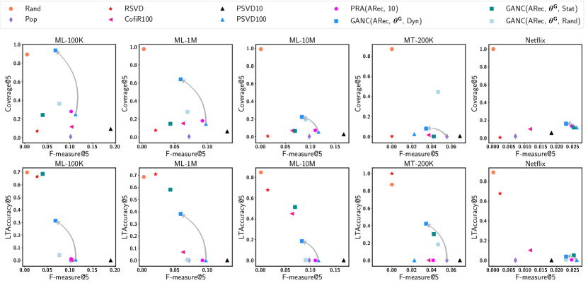
(a)

Figure 6: Accuracy vs Coverage vs Novelty. The head of the arrow shows our main model GANC(ARec, $\bm{\theta}^{G}$, Dyn) with sample size $S=500$, while the bottom shows the underlying accuracy recommender (ARec). On MT-200K ARec is Pop. On other datasets it is PSVD-100. Note, RSVD is consistently dominated by all other models in F-measure and coverage.

As shown previously, in sparse settings, re-ranking frameworks that rely on rating prediction models do not generate accurate solutions. In this section we plug-in a different accuracy recommender w.r.t. dataset density. On MT-200K, we plug-in Pop. On all other datasets we plug-in PSVD100 as the accuracy recommender. For GANC, we use three variants which differ in their coverage recommender: GANC(ARec, $\bm{\theta}^{G}$, Dyn), GANC(ARec, $\bm{\theta}^{G}$, Stat) and GANC(ARec, $\bm{\theta}^{G}$, Rand). We also compare to the generic re-ranking framework, PRA(ARec, 10). For both GANC and PRA, we always plug-in the same accuracy recommender. Furthermore, we compare with standard top-$N$ recommendation algorithms: Rand, Pop, RSVD, CofiR100, PSVD10, PSVD100.

Figure 6 compares accuracy, coverage and novelty trade-offs. On all datasets, Rand achieves the best coverage and gini, but the lowest accuracy. Similar to [1, 5], we find the non-personalized method Pop, which takes advantage of the popularity bias of the data, is a strong contender in accuracy, but under-performs in coverage and novelty.

Regarding GANC, Figure 6 shows the best improvements in coverage are obtained when we use either Rand or Dyn coverage recommenders. Stat is generally not a strong coverage recommender, e.g, GANC(ARec, $\bm{\theta}^{G}$, Stat) obtains high novelty (LTAccuracy) on ML-10M, but does not lead to significant improvements in coverage. This is because Stat has constant gain for long-tail promotion and focuses exclusively on recommending (a small subset of the) long-tail items. Our main model is GANC(ARec, $\bm{\theta}^{G}$, Dyn). An interesting observation is that on MT-200K, both GANC(ARec, $\bm{\theta}^{G}$, Dyn) and GANC(ARec, $\bm{\theta}^{G}$, Rand), that use the non-personalized accuracy recommender Pop as ARec, are competitive with algorithms like PSVD100 or CofiR100.

VI Related Work

We provide an overview of related work here. A detailed description of baselines and methods integrated in our framework is provided in Section IV.

Accuracy-focused rating prediction CF models aim to accurately predict unobserved user ratings [47, 3]. Accuracy is measured using error metrics such as RMSE or Mean Absolute Error that are defined w.r.t. the observed user feedback. Generally, these methods are grouped into memory-based or model-based [47]. Earlier memory-based or neighbourhood models used the rating data directly to compute similarities between users [48] or items [49]. However, these models are not scalable on large-scale datasets like Netflix. Model-based methods instead train a parametric model on the user-item matrix. Matrix Factorization models [47, 40], a.k.a. Singular Value Decomposition (SVD) models, belong to this group and are known for both scalablility and accuracy [1]. These models factorize the user-item matrix into a product of two matrices; one maps the users ($\mathcal{U}$), and the other maps items ($\mathcal{I}$), into a latent factor space of dimension $g\ll\min(|\mathcal{U}|,|\mathcal{I}|)$. Here, each user $u$, and each item $i$, are represented by a factor vector, $\mathbf{p}_{u}\in\mathbb{R}^{g}$, and $\mathbf{q}_{i}\in\mathbb{R}^{g}$, respectively. Ratings are estimated using $\hat{r}_{ui}=\mathbf{q}^{T}_{i}\mathbf{p}_{u}$. Due to the large number of missing values in the user-item matrix, the regularized squared error on the observed ratings is minimized. The resulting objective function is non-convex, and iterative methods such as Stochastic Gradient Descent (SGD) or Alternating Least Squares (ALS) [40, 50, 51] can be used to find a local minimum. From this group, we use RSVD and RSVDN [40, 28], in Section IV.

Accuracy-focused ranking prediction CF models focus on accurately compiling ranked lists. The intuition is that since predicted rating values are not shown to the user, the focus should be on accurately selecting and ranking items. Accordingly, accuracy is measured using ranking metrics, like recall and precision, that can be measured either on the observed user feedback, or on all items [1, 36]. For ranking tasks, Pop obtains high precision and recall [1, 5]. PSVD [1] and CoFiRank [41] are well-known latent factor models for ranking, with others in [43, 35]. We use Pop, PSVD, and CofiRank in Section IV.

Multi-objective methods devise new models that optimize several objectives, like coverage and novelty, in addition to accuracy [5, 6, 13, 38, 52]. In [38], items are assumed to be similar if they significantly co-occur with the same items. This leads to better representations for long-tail items, and increases their chances of being recommended. A new performance measure that combines accuracy and popularity bias is proposed in [6]. This measure can be gradually tuned towards recommending long-tail items. More recently, the idea of recommending users to items as a means of improving sales diversity, and implicitly, recommendation novelty, while retaining precision, has been explored in [5]. In comparison to both [6, 38], we focus on targeted promotion of long-tail items. While [5] focuses on neighbourhood models for top-$N$ recommendation, our framework is generic and independent of the recommender models. Graph-based approaches for long-tail item promotion are studied in [13, 52]. They construct a bipartite user-item graph and use a random walk to trade-off between popular and long-tail items. Rather than devise new multi-objective models, we post-process existing models.

Re-ranking methods post-process the output of a standard model to account for additional objectives like coverage and diversity rather than devising a new model. These algorithms are very efficient. [9] explores re-ranking to maximize diversity within individual top-$N$. It shows that users preferred diversified lists despite their lower accuracy. However, diversifying individual top-$N$ sets does not necessarily increase coverage [17, 38]. Re-ranking techniques that directly maximize coverage and promote long-tail items are explored in [11, 14, 20, 22]. In contrast to [11, 14, 20] that re-rank rating prediction models, our framework is generic and is independent of the base recommendation model. Furthermore, our long-tail personalization is independently learned from interaction data. PRA [22] is also generic framework for re-ranking, although we differ in our long-tail novelty prefernce modelling. We use RBT [14], Resource allocation [20], PRA [22] as baselines since we share similar objectives.

Modelling user novelty preference is studied in [17, 22, 53, 54, 55]. As explained in [53], an item can be novel in three ways: 1. it is new to the system and is unlikely to be seen by most users (cold-start), 2. it existed in the system but is new to a single user, 3. it existed in the system, was previously known by the user, but is a forgotten item. [53, 55] focus on definitions 2 and 3 of novelty, which are useful in settings where seen items can be recommended again, e.g., music recommendation. For defining users’ novelty preferences, tag and temporal data are used in [53, 55]. A logistic regression model is used to predict user novelty preferences in [53], while [55] learn a curiosity model for each user based on her access history and item tags. In [54], gross movie earnings are assumed to reflect movie popularity, and are used to define a personal popularity tendency (PPT) for each user. The idea is to match the PPT of each user with the PPT of recommended items [54]. The major difference between our work and [53, 54, 55] is that we focus on the cold-start definition of novelty (definition 1), we do not use contextual or temporal information to define users’ tendencies for novelty, and we consider domains where each item is accessed at most once (seen items cannot be recommended).

In [17], users are characterized based on their tendency towards disputed items, defined as items with high average rating and high variance. These items are claimed to be in the long-tail. We differ in terms of long-tail novelty definition, and consequently our preference estimates. Furthermore, [17] independently solve a constrained convex optimization problem for each user, with the user’s disputed item tendency as a constraint. [18, 19] use a user risk indicator to decide between a personalized and a non-personalized model; both focus on accuracy. In contrast, we combine accuracy and coverage models. Furthermore, while their risk indicators are optimized via cross validation, we learn the users’ long-tail preferences.

PRA [22] models user preference for long-tail novelty using on item popularity statistics. In contrast, we consider additional information, like if the user found the item interesting, and the long-tail preferences of other users of the item.

CF interaction data properties and test ranking protocol are two important aspects to consider in recommendation setting. CF interaction data suffers from popularity bias [37]. In the movie rating domain, for instance, users are more likely to rate movies they know and like [1, 6, 36, 37, 46]. As a result, the partially observed interaction data is not a random subset of the (unavailable) complete interaction data. Furthermore, many real-world CF interaction datasets [33, 4, 21, 56] are sparse, and the majority of items and users have few observations available. Due to the popularity bias and sparsity of datasets, many accuracy-focused CF models are also biased toward recommending popular items.

Moreover, some accuracy evaluation protocols are also biased and tend to reward popularity biased algorithms [1, 5, 36]. In [36], the main evaluation protocols are assessed in detail, and the “All unrated items test ranking protocol” is described to be closer to the accuracy the user experience in real-world recommendation setting, where performance is measured using the complete data rather than available data [36]. Following [36, 5], and w.r.t. the additional experiments we conducted in Appendix -C, we chose the “All unrated items test ranking protocol” for experiments in Section IV.

VII Conclusion

This paper presents a generic top-$N$ recommendation framework for trading-off accuracy, novelty, and coverage. To achieve this, we profile the users according to their preference for long-tail novelty. We examine various measures, and formulate an optimization problem to learn these user preferences from interaction data. We then integrate the user preference estimates in our generic framework, GANC. Extensive experiments on several datasets confirm that there are trade-offs between accuracy, coverage, and novelty. Almost all re-ranking models increase coverage and novelty at the cost of accuracy. However, existing re-ranking models typically rely on rating prediction models, and are hence more effective in dense settings. Using a generic approach, we can easily incorporate a suitable base accuracy recommender to devise an effective solution for both sparse and dense settings. Although we integrated the long-tail novelty preference estimates into a re-ranking framework, their use-case is not limited to these frameworks. In the future, we intend to explore the temporal and topical dynamics of long-tail novelty preference, particularly in settings where contextual information is available.

Acknowldegments

We thank Glenn Bevilacqua, Neda Zolaktaf, Sharan Vaswani, Mark Schmidt, Laks V. S. Lakshmanan, and Tamara Munzner for their help and valuable discussions. We also thank the anonymous reviewers for their constructive feedback. This work has been funded by NSERC Canada, and supported in part by the Institute for Computing, Information and Cognitive Systems at UBC.

-A Regularized SVD configuration

	R-SVD				R-SVDN
Dataset	$\eta$	$\lambda$	$g$	RMSE	$\eta$	$\lambda$	$g$	RMSE
ML-100K	0.03	0.05	100	0.935	0.03	0.05	100	0.935
ML-1M	0.03	0.05	100	0.868	0.03	0.05	100	0.875
ML-10M	0.003	0.005	20	0.872	0.003	0.005	20	0.872
MT-200k	0.01	0.01	40	0.761	0.01	0.01	40	0.761
Netflix	0.002	0.05	100	0.979	0.002	0.05	100	0.979

TABLE V: R-SVD and R-SVDN parameters on different datasets. $g$ is the number of latent factors, $\eta$ is the learning rate, $\lambda$ is the L2-reqularization coefficient.

Table V provides details for the setup of Regularized SVD (R-SVD) and the same model with non-negative constraints (R-SVDN). We use LIBMF [28] with L2-Norm as the loss function, and L2-regularization, and SGD for optimization. We performed 10-fold cross validation and tested: number of latent factors $g\in\{8,20,40,50,80,100\}$, L2-regularization coefficients $\lambda\in\{0.001,0.005,0.01,0.05,0.1\}$, learning rate $\eta\in\{0.002,0.003,0.01,0.03\}$. For each dataset, we used the parameters that led to best performance.

-B Analysis of Fully Sequential Dynamic Coverage

In this section, we show the problem of finding a top-$N$ collection $\mathcal{P}=\{\mathcal{P}_{u}\}_{u=1}^{|\mathcal{U}|}$ that maximizes Eq. III.2, is an instance of maximizing a submodular function subject to a matroid constraint.

Matroids. A set system is a pair ($\mathcal{I},\mathcal{F}$), where $\mathcal{I}$ denotes a ground set of elements and $\mathcal{F}=\{\mathcal{A}:\mathcal{A}\subseteq\mathcal{I}\}$, is a collection of subsets of $\mathcal{I}$. A set system is an independence system if it satisfies 1. $\emptyset\in\mathcal{F}$, 2. $\mathcal{A}\subseteq\mathcal{B}\in\mathcal{F}\text{ then }\mathcal{A}\in\mathcal{F}$. A matroid is an independence system that also satisfies the property $\mathcal{A},\mathcal{B}\in\mathcal{F}\text{ and }|\mathcal{B}|>|\mathcal{A}|\text{ then }\exists i\in\mathcal{B}\setminus\mathcal{A}\text{ with }\mathcal{A}\cup\{i\}\in\mathcal{F}$. A uniform matroid, is a special class of matroids that satisfies $\mathcal{F}=\{\mathcal{A}:\mathcal{A}\subseteq\mathcal{I},|\mathcal{A}|\leq N\}$, that is all basis are maximal. A partition matroid satisfies $\mathcal{F}=\{\mathcal{A}:\mathcal{A}=\cup_{i=1}^{N}\mathcal{A}_{i},\mathcal{A}_{i}\subseteq\mathcal{I}_{i},|\mathcal{A}_{i}|\leq l_{i},\cup\mathcal{I}_{i}=\mathcal{I}\}$.

Lemma .1.

The constraint of recommending $N$ items to each user, corresponds to a partition matroid over the users.

Proof.

Define a new ground set $\mathcal{N}=\{(u,i):u\in\mathcal{U},i\in\mathcal{I}\}$. Define $\mathcal{N}_{u}=\{(u,i):i\in\mathcal{I}\},u\in\mathcal{U}$ and let $l_{u}=N,\forall u\in\mathcal{U}$. Let $\mathcal{M}=(\mathcal{U},\mathcal{F})$ where $\mathcal{F}=\{\mathcal{P}^{{}^{\prime}}:\mathcal{P}^{{}^{\prime}}=\cup_{u\in\mathcal{U}}\mathcal{P}^{{}^{\prime}}_{u},\mathcal{P}^{{}^{\prime}}_{u}\subseteq\mathcal{N}_{u},|\mathcal{P}^{{}^{\prime}}_{u}|\leq l_{u},\cup\mathcal{N}_{u}=\mathcal{N}\}$. $\mathcal{P}^{{}^{\prime}}$ form independent sets of a partition matroid. ∎

Submodularity and Monotonicity. Let $\mathcal{I}$ denote a ground set of items. Given a set function $f:2^{\mathcal{I}}\rightarrow\mathbb{R}$, $\delta(i|\mathcal{A}):=f(\mathcal{A}\cup\{i\})-f(\mathcal{A})$ is the marginal gain of $f$ at $\mathcal{A}$ with regard to item $i$. Furthermore, $f$ is submodular if and only if $\delta(i|\mathcal{A})\geq\delta(i|\mathcal{B}),\forall\mathcal{A}\subseteq\mathcal{B}\subseteq\mathcal{I},\forall i\in\mathcal{I}\setminus\mathcal{B}$. It is modular if $f(\mathcal{A}\cup{i})$ = $f(\mathcal{A})+f(i)$, $\forall\mathcal{A}\subset\mathcal{I},i\in\mathcal{I}\setminus\mathcal{A}$. In addition, $f$ is monotone increasing if $f(\mathcal{A})\leq f(\mathcal{B}),\forall\mathcal{A}\subseteq\mathcal{B}\subseteq\mathcal{I}$. Equivalently, a function is monotone increasing if and only if $\forall\mathcal{A}\subseteq\mathcal{I}$ and $i\in\mathcal{I}$, $\delta(i|\mathcal{A})\geq 0$ [57]. Submodular functions have the following concave composition property:

Theorem .1.

Using dynamic coverage, the objective function $v(.)$ in Eq.III.2 is submodular monotone increasing w.r.t. sets of user-item pairs.

Proof.

Consider the ground set $\mathcal{N}$, defined in Lemma .1. Based on any set $\mathcal{P}^{{}^{\prime}}\subseteq\mathcal{N}$, define $\mathcal{P}^{{}^{\prime}}_{u}=\{i|(u,i)\in\mathcal{P}^{{}^{\prime}}\}$. We can rewrite the objective function with dynamic coverage as

$$v(\mathcal{P}^{{}^{\prime}}) =\sum_{u}v_{u}(\mathcal{P}^{{}^{\prime}}_{u})$$

$$=\sum_{u}(1-\theta_{u})a(\mathcal{P}^{{}^{\prime}}_{u})+\theta_{u}c(\mathcal{P}^{{}^{\prime}}_{u})$$

$$=\sum_{u}(1-\theta_{u})\sum_{i\in\mathcal{P}^{{}^{\prime}}_{u}}a(i)+\theta_{u}\sum_{i\in\mathcal{P}^{{}^{\prime}}_{u}}c(i)$$ (.1)

$$=\sum_{u}(1-\theta_{u})\sum_{i\in\mathcal{P}^{{}^{\prime}}_{u}}\hat{r}_{ui}+\theta_{u}\sum_{i\in\mathcal{P}^{{}^{\prime}}_{u}}\frac{1}{\sqrt{1+f_{i}^{\mathcal{P}^{{}^{\prime}}}}}$$ (.2)

where $f_{i}^{\mathcal{P}^{{}^{\prime}}}$ is the number of times item $i$ is recommended in $\mathcal{P}^{{}^{\prime}}$. For submodularity consider any $\mathcal{A}\subseteq\mathcal{B}\subset\mathcal{N}$, and a pair $(u,i)\in\mathcal{N}\setminus\mathcal{B}$. We have

$$f_{i}^{\mathcal{A}} \leq f^{\mathcal{B}}_{i}$$

$$\frac{1}{\sqrt{1+f_{i}^{\mathcal{A}}}} \geq\frac{1}{\sqrt{1+f^{\mathcal{B}}_{i}}}$$

$$(1-\theta_{u})\hat{r}_{ui}+\theta_{u}\frac{1}{\sqrt{1+f_{i}^{\mathcal{A}}}} \geq(1-\theta_{u})\hat{r}_{ui}+\theta_{u}\frac{1}{\sqrt{1+f^{\mathcal{B}}_{i}}}$$

$$\delta(i|\mathcal{A}) \geq\delta(i|\mathcal{B})$$

Therefore, due to the submodularity of the coverage function, the overall value function $v(.)$ is submodular.

For monotonicity, both $a(.)$ and $c(.)$ map a set of items $\mathcal{P}_{u}$ to the $[0,1]$ range, and are additive in terms of the number of items (line .1). So, they are both monotonically increasing, i.e., adding a new element $i\in\mathcal{I}\setminus\mathcal{P}_{u}$ to the set $\mathcal{P}_{u}$ can only increase their value. Since $\theta_{u}$ is also in $[0,1]$, $v_{u}(.)$ is monotonically increasing. $v(.)$ is therefore submodular monotone increasing since it is a sum of submodular monotone increasing functions.∎

-C Effect of test ranking protocol on performance metrics

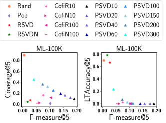
(a) All unrated items ranking protocol

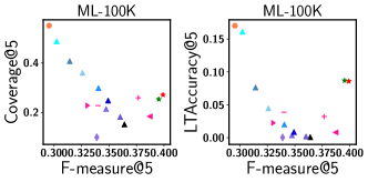
(b) Rated test-items ranking protocol

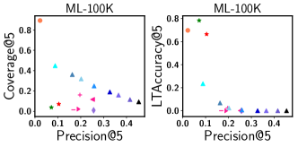
(c) All unrated items ranking protocol

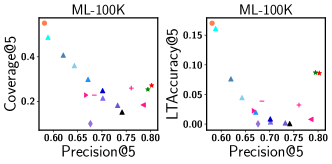
(d) Rated test-items ranking protocol

Figure 7: Comparing the trade-offs for top-5 recommendation, when using different ranking protocols. Dataset is ML-100K.

In our empirical study, we studied off-line recommendation performance of top-$N$ recommendation algorithms from three perspectives: accuracy, novelty, and coverage (Section IV-A). The choice of test ranking protocol [36] is also an important aspect in off-line evaluations. The test ranking protocol describes which items in the test set are ranked for each user [36]. We use the definitions in [36]:

• Rated test-items ranking protocol: for each user, we only rank the observed items in the test set of that user.

• All unrated items ranking protocol: for each user, we rank all items that do not appear in the train set of that user.

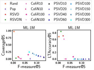
(a) All unrated items ranking protocol

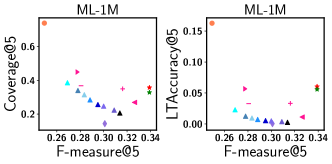
(b) Rated test-items ranking protocol

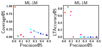
(c) All unrated items ranking protocol

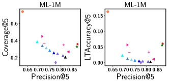
(d) Rated test-items ranking protocol

Figure 8: Comparing the trade-offs for top-5 recommendation, when using different ranking protocols. Dataset is ML-1M.

In [36], it was shown that the choice of test ranking protocol can affect accuracy measurements considerably. Specifically, accuracy is measured either by error metrics (e.g., RMSE and MAE) or ranking metrics (e.g., recall and precision) in recommendation settings  [36]. Error metrics are defined w.r.t. the observed user feedback only. Rating prediction models that optimize these metrics in the train phase, e.g., R-SVD, typically adopt the rated test-items ranking protocol in the test phase. However, error metrics are not precise indicators of accuracy, since they only consider the subset of items that have feedback. But in real-world applications, the system must find and rank a few items ($N$) from among all items [1, 36].

Ranking metrics can be measured on the observed user feedback, or on all items. When measured on the observed user feedback, these metrics can be strongly biased because of the popularity bias of datasets [37, 1, 6, 5, 36]. Therefore, in top-$N$ recommendation settings, these metrics are measured using the all-items ranking protocol, to better reflect accuracy as experienced by users in real-world applications [36, 5].

We extend the empirical study of [36] by evaluating the effect of the test ranking protocol on accuracy, coverage, and novelty. We use standard accuracy-focused CF models (introduced in Section VI). We set $N=5$, and ran experiments on ML-100K and Ml-1M datasets, shown in Figures 7 and 8, respectively.

We analyze Figure 8, which shows the results on the ML-1M dataset (Figure 7 has similar trends). The first observation is that all algorithms obtain higher F-measure scores using the rated test-item ranking protocol. In particular, for the all unrated items ranking protocol, Figure 8.a, F-measure lies in $[0,0.2]$ (with the corresponding precision in $[0,0.5]$ in Figure 8.c ). For the rated test-items ranking protocol F-measure lies in $[0.2,0.4]$ (with precision in $[0.6,0.9]$) . As a specific example, consider Rand which randomly suggests items according to the ranking protocol. As expected, random suggestion from among all items has low F-measure and precision. However, random suggestion from among the test items of each user, leads to an average F-measure of almost $0.25$ (precision approximately $0.6$). This demonstrates the bias of the rated test-items ranking protocol. Similar to [1], we observe Pop is a strong contender in accuracy metrics, using both test protocols [1]. Recent work in [21] also confirmed that Pop outperformed more sophisticated algorithms for tourists datasets, that are sparse and where the users have few and irregular interests (only visit popular locations). In addition, although R-SVD and R-SVDN are less accurate using the all unrated items ranking protocol, they obtain the highest F-measure scores using the rated test-items ranking protocol. This is because these models are optimized w.r.t. the observed user feedback. Therefore, the rated test-items ranking protocol is to their advantage because it also considers only the observed user feedback.

Coverage is also affected by the ranking protocol. The rated test-items ranking protocol results in better coverage for all algorithms except Random. This is because random suggestion from among a user’s test items, is a more constrained algorithm compared to random from among all train items. Regarding the effect of the ranking protocol on LTAccuracy, it lies in $[0,1]$ for the all unrated test items ranking protocol, but drops to $[0,0.2]$ for the rated test-items ranking protocol.

Regarding the trade-off between metrics, irrespective of the ranking protocol, we observe that Pop makes accurate yet trivial recommendations that lack novelty, as indicated by the low LTaccuracy and coverage in Figure 8. For the PureSVD models (P-SVD), on ML-100K and ML-1M, increasing the number of factors reduces F-measure, and results in an increase in coverage and LTAccuracy. Among all baselines, CoFiRank with regression loss (CofiR10, CofiR100) has reasonable coverage, precision, and long-tail accuracy.

Overall, our experiments in this section confirm the findings of prior work [1, 36, 37]: due to the popularity bias of recommendation datasets, rank-based precision is strongly biased when it is measured using the rated test-items ranking protocol. This is demonstrated by the results of Pop, which achieves an F-measure of $0.3$ on ML-100K and ML-1M, with even higher precision scores on those datasets. It outperforms personalized models like CoFiRank. However, using the all-items ranking protocol, the performance of these models aligns better with expectation. Following prior research on top-$N$ recommendation  [36, 5], we conducted the experiments in Section IV using the all-items ranking protocol.

References

- [1] P. Cremonesi, Y. Koren, and R. Turrin, “Performance of recommender algorithms on top-n recommendation tasks,” in RecSys, 2010.
- [2] J. Herlocker, J. A. Konstan, and J. Riedl, “An empirical analysis of design choices in neighborhood-based collaborative filtering algorithms,” Information retrieval, vol. 5, no. 4, 2002.
- [3] J. Lee, M. Sun, and G. Lebanon, “A comparative study of collaborative filtering algorithms,” arXiv preprint arXiv:1205.3193, 2012.
- [4] B. Kanagal, A. Ahmed, S. Pandey, V. Josifovski, J. Yuan, and L. Garcia-Pueyo, “Supercharging recommender systems using taxonomies for learning user purchase behavior,” VLDB, 2012.
- [5] S. Vargas and P. Castells, “Improving sales diversity by recommending users to items,” in RecSys, 2014.
- [6] H. Steck, “Item popularity and recommendation accuracy,” in RecSys, 2011.
- [7] P. Castells, N. J. Hurley, and S. Vargas, Recommender Systems Handbook. Springer US, 2015, ch. Novelty and Diversity in Recommender Systems.
- [8] M. Zhang and N. Hurley, “Avoiding monotony: improving the diversity of recommendation lists,” in RecSys, 2008.
- [9] C.-N. Ziegler, S. M. McNee, J. A. Konstan, and G. Lausen, “Improving recommendation lists through topic diversification,” in WWW, 2005.
- [10] Y. C. Zhang, D. Ó. Séaghdha, D. Quercia, and T. Jambor, “Auralist: introducing serendipity into music recommendation,” in WSDM, 2012.
- [11] G. Adomavicius and Y. Kwon, “Maximizing aggregate recommendation diversity: A graph-theoretic approach,” in International Workshop on Novelty and Diversity in Recommender Systems (DiveRS 2011), 2011.
- [12] C. Anderson, The Long Tail: Why the Future of Business Is Selling Less of More. Hyperion, 2006.
- [13] H. Yin, B. Cui, J. Li, J. Yao, and C. Chen, “Challenging the long tail recommendation,” PVLDB, vol. 5, no. 9, pp. 896–907, 2012.
- [14] G. Adomavicius and Y. Kwon, “Improving aggregate recommendation diversity using ranking-based techniques,” TKDE, 2012.
- [15] M. Ge, C. Delgado-Battenfeld, and D. Jannach, “Beyond accuracy: evaluating recommender systems by coverage and serendipity,” in RecSys, 2010.
- [16] M. Kaminskas and D. Bridge, “Diversity, serendipity, novelty, and coverage: A survey and empirical analysis of beyond-accuracy objectives in recommender systems,” ACM Trans. Interact. Intell. Syst., 2016.
- [17] T. Jambor and J. Wang, “Optimizing multiple objectives in collaborative filtering,” in RecSys, 2010.
- [18] W. Zhang, J. Wang, B. Chen, and X. Zhao, “To personalize or not: a risk management perspective,” in RecSys, 2013, pp. 229–236.
- [19] J. Wang and J. Zhu, “Portfolio theory of information retrieval,” in SIGIR, 2009, pp. 115–122.
- [20] Y.-C. Ho, Y.-T. Chiang, and J. Y.-J. Hsu, “Who likes it more?: mining worth-recommending items from long tails by modeling relative preference,” in WSDM, 2014, pp. 253–262.
- [21] Y. Liu, T.-A. N. Pham, G. Cong, and Q. Yuan, “An experimental evaluation of point-of-interest recommendation in location-based social networks,” Proceedings of the VLDB Endowment, 2017.
- [22] M. Jugovac, D. Jannach, and L. Lerche, “Efficient optimization of multiple recommendation quality factors according to individual user tendencies,” Expert Systems with Applications, vol. 81, 2017.
- [23] D. Agarwal and B.-C. Chen, “Regression-based latent factor models,” in Proceedings of the 15th ACM SIGKDD international conference on Knowledge discovery and data mining. ACM, 2009, pp. 19–28.
- [24] M. Saveski and A. Mantrach, “Item cold-start recommendations: Learning local collective embeddings,” in RecSys, 2014, pp. 89–96.
- [25] G. Salton and C. Buckley, “Term-weighting approaches in automatic text retrieval,” Information processing & management, 1988.
- [26] Y. Li, Q. Li, J. Gao, L. Su, B. Zhao, W. Fan, and J. Han, “On the discovery of evolving truth,” in KDD. ACM, 2015.
- [27] R. Agrawal, S. Gollapudi, A. Halverson, and S. Ieong, “Diversifying search results,” in WSDM, 2009.
- [28] Y. Zhuang, W.-S. Chin, Y.-C. Juan, and C.-J. Lin, “A fast parallel sgd for matrix factorization in shared memory systems,” in RecSys, 2013.
- [29] S. Khuller, A. Moss, and J. S. Naor, “The budgeted maximum coverage problem,” Information Processing Letters, vol. 70, no. 1, 1999.
- [30] M. L. Fisher, G. L. Nemhauser, and L. A. Wolsey, An analysis of approximations for maximizing submodular set functions-II. Springer, 1978.
- [31] S. J. Sheather and M. C. Jones, “A reliable data-based bandwidth selection method for kernel density estimation,” Journal of the Royal Statistical Society. Series B (Methodological), pp. 683–690, 1991.
- [32] F. M. Harper and J. A. Konstan, “The movielens datasets: History and context,” ACM Trans. on Interactive Intelligent Systems (TiiS), 2016.
- [33] S. Dooms, T. De Pessemier, and L. Martens, “Movietweetings: a movie rating dataset collected from twitter,” in CrowdRec at RecSys, 2013.
- [34] J. M. Hernandez-lobato, N. Houlsby, and Z. Ghahramani, “Probabilistic matrix factorization with non-random missing data,” in ICML, 2014.
- [35] J. Lee, S. Bengio, S. Kim, G. Lebanon, and Y. Singer, “Local collaborative ranking,” in WWW, 2014, pp. 85–96.
- [36] H. Steck, “Evaluation of recommendations: rating-prediction and ranking,” in Proceedings of the 7th ACM conference on Recommender systems. ACM, 2013, pp. 213–220.
- [37] D. K. Agarwal and B.-C. Chen, Statistical Methods for Recommender Systems. Cambridge University Press, 2016.
- [38] K. Niemann and M. Wolpers, “A new collaborative filtering approach for increasing the aggregate diversity of recommender systems,” in SIGKDD, 2013, pp. 955–963.
- [39] M. O. Lorenz, “Methods of measuring the concentration of wealth,” Publications of the American Statistical Association, 1905.
- [40] Y. Koren, R. Bell, and C. Volinsky, “Matrix factorization techniques for recommender systems,” Computer, no. 8, pp. 30–37, 2009.
- [41] M. Weimer, A. Karatzoglou, Q. V. Le, and A. Smola, “Maximum margin matrix factorization for collaborative ranking,” Advances in neural information processing systems, pp. 1–8, 2007.
- [42] E. M. Voorhees, “Overview of trec 2001,” in Trec, 2001.
- [43] S. Balakrishnan and S. Chopra, “Collaborative ranking,” in WSDM, 2012.
- [44] M. Volkovs and R. S. Zemel, “Collaborative ranking with 17 parameters,” in Advances in Neural Information Processing Systems, 2012, pp. 2294–2302.
- [45] B. M. Marlin, R. S. Zemel, S. Roweis, and M. Slaney, “Collaborative filtering and the missing at random assumption,” in UAI, 2007.
- [46] H. Steck, “Training and testing of recommender systems on data missing not at random,” in SIGKDD, 2010.
- [47] Y. Koren, “Factorization meets the neighborhood: a multifaceted collaborative filtering model,” in SIGKDD, 2008.
- [48] J. L. Herlocker, J. A. Konstan, A. Borchers, and J. Riedl, “An algorithmic framework for performing collaborative filtering,” in SIGIR, 1999.
- [49] B. Sarwar, G. Karypis, J. Konstan, and J. Riedl, “Item-based collaborative filtering recommendation algorithms,” in WWW, 2001.
- [50] A. Mnih and R. Salakhutdinov, “Probabilistic matrix factorization,” in Advances in neural information processing systems, 2007.
- [51] S. Rendle, “Factorization machines with libFM,” ACM Trans. on Intelligent Systems and Technology, vol. 3, no. 3, pp. 1–22, May 2012.
- [52] L. Shi, “Trading-off among accuracy, similarity, diversity, and long-tail: A graph-based recommendation approach,” in RecSys, 2013, pp. 57–64.
- [53] K. Kapoor, V. Kumar, L. Terveen, J. A. Konstan, and P. Schrater, “I like to explore sometimes: Adapting to dynamic user novelty preferences,” in Proceedings of the 9th ACM Conference on Recommender Systems. ACM, 2015, pp. 19–26.
- [54] J. Oh, S. Park, H. Yu, M. Song, and S.-T. Park, “Novel recommendation based on personal popularity tendency,” in Data Mining (ICDM), 2011 IEEE 11th International Conference on. IEEE, 2011, pp. 507–516.
- [55] P. Zhao and D. L. Lee, “How much novelty is relevant?: It depends on your curiosity,” in SIGIR. ACM, 2016.
- [56] S. Zolaktaf and G. C. Murphy, “What to learn next: Recommending commands in a feature-rich environment,” in IEEE International Conference on Machine Learning and Applications (ICMLA). IEEE, 2015.
- [57] A. Krause and D. Golovin, “Submodular function maximization.”