Neural Networks Should Be Wide Enough to Learn Disconnected Decision Regions
Abstract
In the recent literature the important role of depth in deep learning has been emphasized. In this paper we argue that sufficient width of a feedforward network is equally important by answering the simple question under which conditions the decision regions of a neural network are connected. It turns out that for a class of activation functions including leaky ReLU, neural networks having a pyramidal structure, that is no layer has more hidden units than the input dimension, produce necessarily connected decision regions. This implies that a sufficiently wide hidden layer is necessary to guarantee that the network can produce disconnected decision regions. We discuss the implications of this result for the construction of neural networks, in particular the relation to the problem of adversarial manipulation of classifiers.
1 Introduction
While deep learning has become state of the art in many application domains such as computer vision and natural language processing and speech recognition, the theoretical understanding of this success is steadily growing but there are still plenty of questions where there is little or no understanding. In particular, for the question how one should construct the network e.g. choice of activation function, number of layers, number of hidden units per layer etc., there is little guidance and only limited understanding on the implications of the choice e.g. “The design of hidden units is an extremely active area of research and does not yet have many definitive guiding theoretical principles.” is a quote from the recent book on deep learning (Goodfellow et al., 2016, p. 191). Nevertheless there is recently progress in the understanding of these choices.
The first important results are the universal approximation theorems (Cybenko, 1989; Hornik et al., 1989) which show that even a single hidden layer network with standard non-polynomial activation function (Leshno et al., 1993), like the sigmoid, can approximate arbitrarily well every continuous function over a compact domain of . In order to explain the success of deep learning, much of the recent effort has been spent on analyzing the representation power of neural networks from the perspective of depth (Delalleau & Bengio, 2011; Telgarsky, 2016, 2015; Eldan & Shamir, 2016; Safran & Shamir, 2017; Yarotsky, 2016; Poggio et al., 2016; Liang & Srikant, 2017; Mhaskar & Poggio, 2016). Basically, they show that there exist functions that can be computed efficiently by deep networks of linear or polynomial size but require exponential size for shallow networks. To further highlight the power of depth, (Montufar et al., 2014; Pascanu et al., 2014) show that the number of linear regions that a ReLU network can form in the input space grows exponentially with depth. Tighter bounds on the number of linear regions are later on developed by (Arora et al., 2018; Serra et al., 2018; Charisopoulos & Maragos, 2018). Another measure of expressivity so-called trajectory length is proposed by (Raghu et al., 2017). They show that the complexity of functions computed by the network along a one-dimensional curve in the input space also grows exponentially with depth.
While most of previous work can only show the existence of depth efficiency (i.e. there exist certain functions that can be efficiently represented by deep networks but not effectively represented or even approximated by shallow networks) but cannot show how often this holds for all functions of interest, (Cohen et al., 2016) have taken the first step to address this problem. In particular, by studying a special type of networks called convolutional arithmetic circuits – also known as Sum-Product networks (Poon & Domingos, 2011), the authors show that besides a set of measure zero, all functions that can be realized by a deep network of polynomial size require exponential size in order to be realized, or even approximated by a shallow network. Later, (Cohen & Shashua, 2016) show that this property however no longer holds for convolutional rectifier networks, which represents so far the empirically most successful deep learning architecture in practice.
Unlike most of previous work which focuses on the power of depth, (Lu et al., 2017; Hanin & Sellke, 2017) have recently shown that neural networks with ReLU activation function have to be wide enough in order to have the universal approximation property as depth increases. In particular, the authors show that the class of continuous functions on a compact set cannot be arbitrarily well approximated by an arbitrarily deep network if the maximum width of the network is not larger than the input dimension . Moreover, it has been shown recently, that the loss surface of fully connected networks (Nguyen & Hein, 2017) and for convolutional neural networks (Nguyen & Hein, 2018) is well behaved, in the sense that almost all local minima are global minima, if there exists a layer which has more hidden units than the number of training points.
In this paper we study the question under which conditions on the network the decision regions of a neural network are connected respectively can potentially be disconnected. The decision region of a class is the subset of , where the network predicts this class. A similar study has been in (Makhoul et al., 1989, 1990) for feedforward networks with threshold activation functions, where they show that the initial layer has to have width in order that one can get disconnected decision regions. On an empirical level it has recently been argued (Fawzi et al., 2017) that the decision regions of the Caffe Network (Jia et al., 2014) on ImageNet are connected. In this paper we analyze feedforward networks with continuous activation functions as currently used in practice. We show in line with previous work that almost all networks which have a pyramidal structure up to the last hidden layer, that is the width of all hidden layers is smaller than the input dimension , can only produce connected decision regions. We show that the result is tight by providing explicit counterexamples for the case . We conclude that a guiding principle for the construction of neural networks should be that there is a layer which is wider than the input dimension as it would be a strong assumption that the Bayes optimal classifier must have connected decision regions. Interestingly, our result holds for leaky ReLU, that is for , whereas the result of (Hanin & Sellke, 2017) is for ReLU, that is , but “the generalization is not straightforward, even for activations of the form , where are affine functions with different slopes.” We discuss also the implications of connected decision regions regarding the generation of adversarial samples, which will provide another argument in favor of larger width for neural network architectures.
2 Feedforward Neural Networks
We consider in this paper feedforward neural networks for multi-class classification. Let be the input dimension and the number of classes. Let be the number of layers where the layers are indexed from which respectively corresponds to the input layer, 1st hidden layer, , and the output layer . Let be the width of layer . For consistency, we assume that and . Let be the activation function of every hidden layer . In the following, all functions are applied componentwise. We define as the feature map of layer , which computes for every input a feature vector at layer defined as
where is the weight matrix at layer . Please note that the output layer is linear as it is usually done in practice. We consider in the following activation functions which are continuous and strictly monotonically increasing. This is true for most of proposed activation functions, but does not hold for ReLU, . On the other hand, it has been argued in the recent literature, that the following variants are to be preferred over ReLU as they deal better with the vanishing gradient problem and outperform ReLU in prediction performance (He et al., 2015; Clevert et al., 2016). This is leaky ReLU (Maas et al., 2013):
where typically is fixed but it has also been optimized together with the network weights (He et al., 2015) and ELU (exponential linear unit) (Clevert et al., 2016):
Note that image of the activation function , , is equal to for leaky ReLU and for the exponential linear unit.
3 Connectivity of Decision Regions
In this section, we prove two results on the connectivity of the decision regions of a classifier. Both require that the activation function is continuous and strictly monotonically increasing. Our main Theorem 3.10 holds for feedforward networks of arbitrary depth and requires additionally , the second Theorem 3.11 holds just for one hidden layer networks but has no further requirements on the activation function. Both show that in general pyramidal feedforward neural networks where the width of all the hidden layers is smaller than or equal to the input dimension can only produce connected decision regions.
3.1 Preliminary technical results
We first introduce the definitions and terminologies used in the following, before we prove or recall some simple results about continuous mappings from to . For a function , where and , we denote for every subset , the image as Let
Definition 3.1 (Decision region)
The decision region of a given class , denoted by , is defined as
Definition 3.2 (Connected set)
A subset is called connected if for every , there exists a continuous curve such that and
To prove our key Lemma 3.9, the following properties of connected sets and continuous functions are useful. All proofs are moved to the appendix due to limited space.
Proposition 3.3
Let be a continuous function. If is a connected set then is also a connected set.
Proposition 3.4
The Minkowski sum of two connected subsets , defined as , is a connected set.
As our main idea is to transfer the connectedness of a set from the output layer back to the input layer, we require the notion of pre-image and inverse mapping.
Definition 3.5 (Pre-Image)
The pre-image of a function is the set-valued function defined for every as
Similarly, for every subset , let
By definition, it holds for every subset that if and only if Moreover, for every
As a deep feedforward network is a composition of the individual layer functions, we need the following property.
Proposition 3.6
Let and be two functions. Then it holds that
Apart from the property of connectivity, we can also show the openness of a set when considering the pre-image of a given network. We recall the following standard result from topology (see e.g. Apostol, 1974, Theorem 4.23, p. 82).
Proposition 3.7
Let be a continuous function. If is an open set then is also open.
We now recall a standard result from calculus showing that under certain, restricted conditions the inverse of a continuous mapping exists and is as well continuous.
Proposition 3.8
Let be continuous and strictly monotonically increasing. Then the inverse mapping exists and is continuous.
The following lemma is a key ingredient in the following proofs. It allows us to show that the pre-image of an open and connected set by a one hidden layer network is again open and connected. Using the fact that deep networks can be seen as a composition of such individual layers, this will later on allow us to transfer the result to deep networks.
Lemma 3.9
Let and be a function defined as where is defined as
| (1) |
and is bijective, continuous and strictly monotonically increasing, is a linear map defined as where has full rank and If is an open connected set then is also an open connected set.
Proof: By Proposition 3.6, it holds that As is a componentwise function, the inverse mapping is given by the inverse mappings of the components
where under the stated assumptions the inverse mapping exists by Lemma 3.8 and is continuous. Since , is the image of the connected set under the continuous map . Thus by Proposition 3.3, is connected. Moreover, is an open set by Proposition 3.7.
It holds for every that
where the inverse of exists as has full rank (note that we assume ). As has full rank and , it holds that and thus
Therefore it holds for that
where the first term is the image of the connected set
under an affine mapping and thus is again connected by Proposition 3.3,
the second term is a linear subspace which is also connected.
By Proposition 3.4, the Minkowski sum of two connected sets is connected.
Thus is a connected set.
Moreover, as is the pre-image of the open set under the continuous function ,
it must be also an open set by Proposition 3.7.
Thus is an open and connected set.
Note that in Lemma 3.9, if and has full rank then and the linear equation
has a unique solution for every and thus
In this case, even though is a connected set, the intersection can be disconnected which can imply that is disconnected and thus the decision region becomes disconnected.
We illustrate this with a simple example, where and with and and . In this case it holds that
| (2) |
Figure 1 shows that is a one-dimensional submanifold (in this case subspace) of and provides an example of a set where the pre-image is disconnected.
3.2 Main results
We show in the following that the decisions regions of feedforward networks which are pyramidal and have maximal width at most the input dimension can only produce connected decision regions. We assume for the activation functions that , which is fulfilled by leaky ReLU.
Theorem 3.10
Let the width of the layers of the feedforward network network satisfy and let be a continuous, strictly monotonically increasing function with for every layer and all the weight matrices have full rank. Then every decision region is an open connected subset of for every
Proof: From Definition 3.1, it holds for every
where
Let us define the set
then it holds If is an empty set then we are done, otherwise one observes that is the intersection of a finite number of open half-spaces (or the whole space), which is thus an open and connected set. Moreover, it holds , where is defined as in (1). It follows from Proposition 3.7 that must be an open set as it is the pre-image of the open set under the continuous mapping To show that is a connected set, one first observes that
where is an affine mapping between layer and layer defined as for every , and is the activation mapping of layer defined as in (1). By Proposition 3.6 it holds that
Since is a continuous bijection by our assumption,
it follows that is also a continuous bijection.
Moreover, it holds that has full rank and for every and is a connected set.
Thus one can apply Lemma 3.9 subsequently for the composed functions
for every and obtains that is a connected set.
Thus is an open and connected set for every
The next theorem holds just for networks with one hidden layer but allows general activation functions which are continuous
and strictly monotonically increasing, that is leaky ReLU, ELU, softplus or sigmoid activation functions. Again the decision
regions are connected if the hidden layer has maximal width smaller than .
Theorem 3.11
Let the one hidden layer network satisfy and let be a continuous, strictly monotonically increasing function and the hidden layer’s weight matrix has full rank. Then every decision region is an open connected subset of for every
Proof: We note that in the proof of Theorem 3.10 the is a finite intersection of open half-spaces and thus a convex set. Moreover, is an open convex set (it is just an axis-aligned open box), as is strictly monotonically increasing. Thus
As both sets are open convex sets, the intersection is again convex and open as well.
Thus is a connected set. The rest of the argument follows then by using Lemma 3.9,
noting that by Proposition 3.8 is a continuous mapping.
Note that Theorem 3.10 and Theorem 3.11 make no assumption on the structure of all layers in the network.
Thus they can be applied to neural networks with both fully connected layers and convolutional layers.
Moreover, the results hold regardless of how the parameters of the network have been attained,
trained or otherwise, as long as all the weight matrices of hidden layers have full rank.
This is a quite weak condition in practice as the set of low rank matrices has just Lebesgue measure zero. Even if the optimal weight parameters
for the data generating distribution would be low rank (we discuss such an example below), then it is very unlikely that the trained weight parameters are low rank, as one has
statistical noise by the training sample, “optimization noise” from the usage of stochastic gradient descent (SGD)
and its variants and finally
in practice one often uses early stopping and thus even if the optimal solution for the training set is low rank,
one will not find it.
Theorem 3.10 covers activation functions like leaky ReLU but not sigmoid, ELU or softplus. At the moment it is unclear for us if the result might hold also for the more general class of activation functions treated in Theorem 3.11. The problem is that then in Lemma 3.9 one has to compute the pre-image of . Even though both sets are connected, the intersection of connected sets need not be connected. This is avoided in Theorem 3.11 by using that the initial set and are both convex and the intersection of convex sets is convex and thus connected.
We show below that the result is tight in the sense that we give an empirical example of a neural network with a single hidden layer of hidden units which produces disconnected regions. Note that our result complements the result of (Hanin & Sellke, 2017), where they show the universal approximation property (for ReLU) only if one considers networks of width at least for arbitrary depth. Theorem 3.10 and Theorem 3.11 indicate that this result could also hold for leaky ReLU as approximation of arbitrary functions implies approximation of arbitrary decisions regions, which clearly requires that one is able to get disconnected decision regions. Taking both results together, it seems rather obvious that as a general guiding principle for the construction of hidden layers in neural networks one should use, at least for the first hidden layer, more units than the input dimension, as it is rather unlikely that the Bayes optimal decision regions are connected. Indeed, if the true decision regions are disconnected then using a network of smaller width than might still perfectly fit the finite training data but since the learned decision regions are connected there exists a path between the true decision regions which then can be used for potential adversarial manipulation. This is discussed in the next section where we show empirical evidence for the existence of such adversarial examples.
4 Illustration and Discussion
In this section we discuss with analytical examples as well as trained networks that the result is tight and the conditions of the theorem cannot be further relaxed. Moreover, we argue that connected decision regions can be problematic as they open up the possibility to generate adversarial examples.
4.1 Why pyramidal structure of the network is necessary to get connected decision regions?
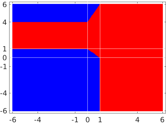
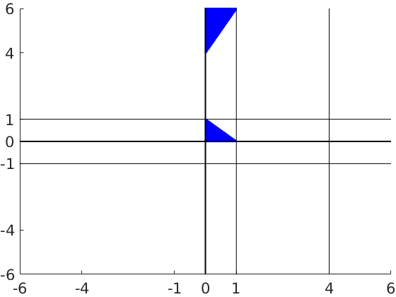
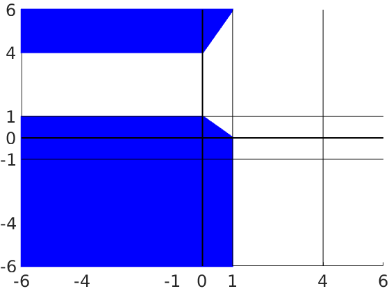
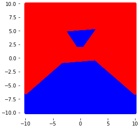
In Theorem 3.10, if the network does not have pyramidal structure up to the last hidden layer, i.e. the condition is not fulfilled, then the statement of the theorem might not hold as the decision regions can be disconnected. We illustrate this via a counter-example below. Let us consider a non-pyramidal network 2-1-2-2 defined as
| (3) |
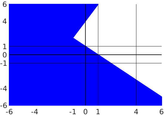
where , and Then one can check that this network has (see appendix for the full derivation) , which is a disconnected set as illustrated in Figure 2.
4.2 Why full rank of the weight matrices is necessary to get connected decision regions?
Similar to Section 4.1, we show that if the weight matrices of hidden layers are not full rank while the other conditions are still satisfied, then the decision regions can be disconnected. The reason is simply that low rank matrices, in particular in the first layer, reduce the effective dimension of the input. We illustrate this effect with a small analytical example and then argue that nevertheless in practice it is extremely difficult to get low rank weight matrices.
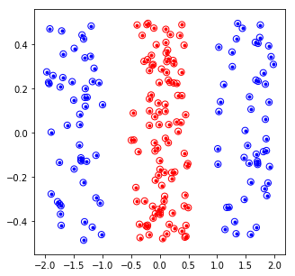
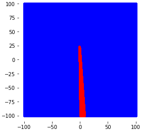
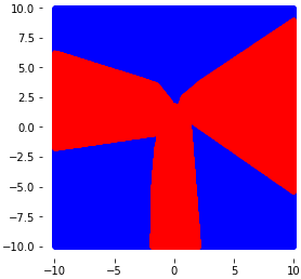
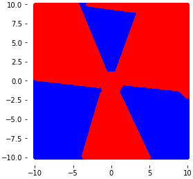
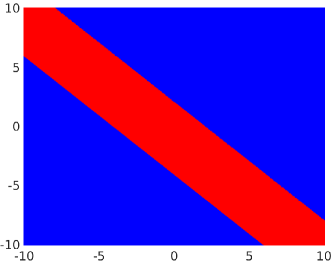
Suppose one has a two-class classification problem on (see Figure 3) with equal class probabilities , and the conditional distribution is given as
| (4) |
Note that the Bayes optimal decision region for class blue is disconnected. Moreover, it is easy to verify that a one hidden layer network with leaky ReLU for can perfectly fit the data with
Note that has low rank. Suppose that the first output unit corresponds to the blue class and second output unit corresponds to the red class. Then it holds , and thus
which implies that for every and thus the decision region for class blue has two disconnected decision regions. This implies that Theorems 3.10 and 3.11 do indeed not hold if the weight matrices do not have full rank. Nevertheless in practice, it is unlikely that one will get such low rank weight matrices, which we illustrate in Figure 3 that the decision regions of the trained classifier has indeed connected decision regions. This is due to statistical noise in the training set as well as through the noise in the optimization procedure (SGD) and the common practice of early stopping in training of neural networks.
4.3 Does the result hold for ReLU activation function?
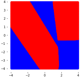
As the conditions of Theorem 3.10 are not fulfilled for ReLU, one might ask whether the decision regions of a ReLU network with pyramidal structure and full rank weight matrices can be potentially disconnected. We show that this is indeed possible via the following example. Let a two hidden layer network (2-2-2-2) be defined as
| (5) |
where and
and Then one can derive the decision region for the first class as (see appendix for the full derivation)
which is a disconnected set as illustrated in Figure 2.
Finally, one notes in this example that except for the activation function, all the other conditions of Theorem 3.10 are still satisfied, that is, the network has pyramidal structure (2-2-2-2) and all the weight matrices have full rank by our construction. Thus the statement of Theorem 3.10, at least under current form, does not hold for ReLU.
4.4 The theorems are tight: disconnected decision regions for width
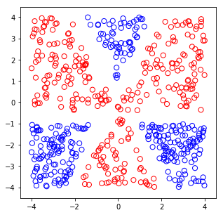
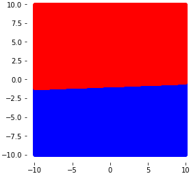
We consider a binary classification task in where the data points are generated so that the blue class has disconnected components on the square , see Figure 4 (a) for an illustration. We use a one hidden layer network with varying number of hidden units, two output units, leaky ReLU activation function and cross-entropy loss. We then train this network by using SGD with momentum for epochs and learning rate and reduce the it by a factor of after every epochs. For all the attempts with different starting points that we have done in our experiment, the resulting weight matrices always have full rank.
We show the training error and the decision regions of trained network in Figure 4. The grid size in each case of Figure 4 has been manually chosen so that one can see clearly the connected/disconnected components in the decision regions. First, we observe that for two hidden units (), the network satisfies the condition of Theorem 3.10 and thus can only learn connected regions, which one can also clearly see in the figure, where one basically gets a linear separator. However, for three hidden units (), one can see that the network can produce disconnected decision regions, which shows that both our Theorems 3.10 and 3.11 are tight, in the sense that width is already sufficient to produce disconnected components, whereas the results say that for width less than the decision regions have to be connected. As the number of hidden units increases, we observe that the network produces more easily disconnected decision regions as expected.
4.5 Relation to adversarial manipulation
We use a single image of digit from the MNIST dataset to create a new artificial dataset where the underlying data generation probability measure has a similar one-dimensional structure as in (4.2) but now embedded in the pixel space . This is achieved by using rotation as the one-dimensional degree of freedom. We generate training images for each red/blue class by rotating the chosen digit with angles ranging from for the read class, and for the blue class, see Figure 5.

\stackunder \stackunder

(source)
\stackunder \stackunder
 \stackunder
 \stackunder
 \stackunder
 \stackunder
 \stackunder
 \stackunder
 \stackunder
 \stackunder
 (adversarial)
\stackunder
 (adversarial)
\stackunder
 \stackunder
 \stackunder
 \stackunder
 \stackunder
 \stackunder
 \stackunder
 \stackunder
 \stackunder
 \stackunder
 (target)

(source)
\stackunder \stackunder
 \stackunder
 \stackunder
 \stackunder
 \stackunder
 \stackunder
 \stackunder
 \stackunder
 \stackunder
 (adversarial)
\stackunder
 (adversarial)
\stackunder
 \stackunder
 \stackunder
 \stackunder
 \stackunder
 \stackunder
 \stackunder
 \stackunder
 \stackunder
 \stackunder
 (target)
Note that this is a binary classification task where the dataset has just one effective degree of freedom and the Bayes optimal decision regions are disconnected. We train a one hidden layer network with hidden units which is equal to the input dimension and leaky ReLU as activation function with . The training error is zero and the resulting weight matrices have full rank, thus the conditions of Theorem 3.10 are satisfied and the decision region of class blue should be connected even though the Bayes optimal decision region is disconnected. This can only happen by establishing a connection around the other red class. We test this by sampling a source image from the part of the blue class and a target image from the other part . Next, we generate an adversarial image 111This is essentially a small perturbation of an image from the red class which is classified as blue class from the red class using the one step target class method (Kurakin et al., 2016, 2017) and consider the path between the source image to the adversarial image and subsequently from the adversarial image to the target one. For each path, we simply consider the line segment for between the two endpoint images and and sample it very densely by dividing into equidistant parts. Figure 6 shows the complete path from the source image to the target image where the color indicates that all the intermediate images are classified as blue with high confidence (note that we turned the output of the network into probabilities by using the softmax function). Moreover, the intermediate images from Figure 6 look very much like images from the red class thus could be seen as adversarial samples for the red class. The point we want to make here is that one might think that in order to avoid adversarial manipulation the solution is to use a simple classifier of low capacity. We think that rather the opposite is true in the sense that only if the classifier is rich enough to model the true underlying data generating distribution it will be able to model the true decision boundaries. In particular, the classifier should be able to realize disconnected decision regions in order to avoid paths through the input space which connect different disconnected regions of the Bayes optimal classifier. Now one could argue that the problem of our synthetic example is that the corresponding digits obviously do not fill the whole image space, nevertheless the classifier has to do a prediction for all possible images. This could be handled by introducing a background class, but then it would be even more important that the classifier can produce disconnected decision regions which naturally requires a minimal width of of the network.
In Figure 7, we show another similar experiment on MNIST dataset, but now for all the image classes. We train a network with hidden units, leaky ReLU and softmax cross-entropy loss to zero training error. Once again, one can see that there exists a continuous path that connects two different-looking images of digit (blue class) where every image along this path is classified as blue class with high confidence. Moreover this path goes through a pre-constructed adversarial image of the red class (digit ).
5 Conclusion
We have shown that deep neural networks (with a certain class of activation functions) need to have in general width larger than the input dimension in order to learn disconnected decision regions. It remains an open problem if our current requirement can be removed. While our result does not resolve the question how to choose the network architecture in practice, it provides at least a guideline how to choose the width of the network. Moreover, our result and experiments show that too narrow networks produce high confidence predictions on a path connecting the true disconnected decision regions which could be used to attack these networks using adversarial manipulation.
Acknowledgements
The authors would like to thank the reviewers for their helpful comments on the paper and Francesco Croce for bringing up a counter-example for the ReLU activation function.
References
- Apostol (1974) Apostol, T. M. Mathematical analysis. Addison Wesley, Reading, Massachusetts, 1974.
- Arora et al. (2018) Arora, R., Basu, A., Mianjy, P., and Mukherjee, A. Understanding deep neural networks with rectified linear units. In ICLR, 2018.
- Charisopoulos & Maragos (2018) Charisopoulos, V. and Maragos, P. A tropical approach to neural networks with piecewise linear activations, 2018. arXiv:1805.08749.
- Clevert et al. (2016) Clevert, D., Unterthiner, T., and Hochreiter, S. Fast and accurate deep network learning by exponential linear units (elus). In ICLR, 2016.
- Cohen & Shashua (2016) Cohen, N. and Shashua, A. Convolutional rectifier networks as generalized tensor decompositions. In ICML, 2016.
- Cohen et al. (2016) Cohen, N., Sharir, O., and Shashua, A. On the expressive power of deep learning: A tensor analysis. In COLT, 2016.
- Cybenko (1989) Cybenko, G. Approximation by superpositions of a sigmoidal function. Mathematics of Control, Signals, and Systems, 2:303–314, 1989.
- Delalleau & Bengio (2011) Delalleau, O. and Bengio, Y. Shallow vs. deep sum-product networks. In NIPS, 2011.
- Eldan & Shamir (2016) Eldan, R. and Shamir, O. The power of depth for feedforward neural networks. In COLT, 2016.
- Fawzi et al. (2017) Fawzi, A., Dezfooli, S. M. M., Frossard, P., and Soatto, S. Classification regions of deep neural networks, 2017. arXiv:1705.09552.
- Goodfellow et al. (2016) Goodfellow, I., Bengio, Y., and Courville, A. Deep Learning. MIT Press, 2016. http://www.deeplearningbook.org.
- Hanin & Sellke (2017) Hanin, B. and Sellke, M. Approximating continuous functions by relu nets of minimal width, 2017. arXiv:1710.11278.
- He et al. (2015) He, K., Zhang, X., Ren, S., and Sun, J. Delving deep into rectifiers: Surpassing human-level performance on imagenet classification. In ICCV, 2015.
- Hornik et al. (1989) Hornik, K., Stinchcombe, M., and White, H. Multilayer feedforward networks are universal approximators. Neural Networks, 2:359–366, 1989.
- Jia et al. (2014) Jia, Y., Shelhamer, E., Donahue, J., Karayev, S., Long, J., Grishick, R., Guadarrama, S., and Darrell, T. Caffe: Convolutional architecture for fast feature embedding. In ACM Int. Conference on Multimedia, 2014.
- Kurakin et al. (2016) Kurakin, A., Goodfellow, I., and Bengio, S. Adversarial machine learning at scale. In ICLR, 2016.
- Kurakin et al. (2017) Kurakin, A., Goodfellow, I., and Bengio, S. Adversarial examples in the physical world. In ICLR Workshop, 2017.
- Leshno et al. (1993) Leshno, M., Lin, Y., Pinkus, A., and Schocken, S. Multilayer feedforward networks with a nonpolynomial activation function can approximate any function. Neural Networks, 6:861–867, 1993.
- Liang & Srikant (2017) Liang, S. and Srikant, R. Why deep neural networks for function approximation? In ICLR, 2017.
- Lu et al. (2017) Lu, Z., Pu, H., Wang, F., Hu, Z., and Wang, L. The expressive power of neural networks: A view from the width. In NIPS, 2017.
- Maas et al. (2013) Maas, A. L., Hannun, A. Y., and Ng, A. Y. Rectifier nonlinearities improve neural network acoustic models. In ICML, 2013.
- Makhoul et al. (1989) Makhoul, J., El-Jaroudi, A., and Schwartz, R. Formation of disconnected decision regions with a single hidden layer. IJCNN, pp. 455–460, 1989.
- Makhoul et al. (1990) Makhoul, J., El-Jaroudi, A., and Schwartz, R. Partitioning capbabilities of two-layer neural networks. IEEE Trans. Signal Processing, 39(6):1435–1440, 1990.
- Mhaskar & Poggio (2016) Mhaskar, H. and Poggio, T. Deep vs. shallow networks : An approximation theory perspective, 2016. arXiv:1608.03287.
- Montufar et al. (2014) Montufar, G., Pascanu, R., Cho, K., and Bengio, Y. On the number of linear regions of deep neural networks. In NIPS, 2014.
- Nguyen & Hein (2017) Nguyen, Q. and Hein, M. The loss surface of deep and wide neural networks. In ICML, 2017.
- Nguyen & Hein (2018) Nguyen, Q. and Hein, M. Optimization landscape and expressivity of deep cnns. In ICML, 2018.
- Pascanu et al. (2014) Pascanu, R., Montufar, G., and Bengio, Y. On the number of response regions of deep feedforward networks with piecewise linear activations. In ICLR, 2014.
- Poggio et al. (2016) Poggio, T., Mhaskar, H., Rosasco, L., Miranda, B., and Liao, Q. Why and when can deep – but not shallow – networks avoid the curse of dimensionality: a review, 2016. arXiv:1611.00740.
- Poon & Domingos (2011) Poon, H. and Domingos, P. Sum-product networks: A new deep architecture. In ICCV Workshop, 2011.
- Raghu et al. (2017) Raghu, M., Poole, B., Kleinberg, J., Ganguli, S., and Sohl-Dickstein, J. On the expressive power of deep neural networks. In ICML, 2017.
- Safran & Shamir (2017) Safran, I. and Shamir, O. Depth-width tradeoffs in approximating natural functions with neural networks. In ICML, 2017.
- Serra et al. (2018) Serra, T., Tjandraatmadja, C., and Ramalingam, S. Bounding and counting linear regions of deep neural networks, 2018. arXiv:1711.02114.
- Telgarsky (2015) Telgarsky, M. Representation benefits of deep feedforward networks, 2015. arXiv:1509.08101v2.
- Telgarsky (2016) Telgarsky, M. Benefits of depth in neural networks. In COLT, 2016.
- Yarotsky (2016) Yarotsky, D. Error bounds for approximations with deep relu networks, 2016. arXiv:1610.01145.
Proof of Proposition 3.3 Pick some Then there must exist some such that and Since is a connected set, it holds by Definition 3.2 that there exists a continuous curve such that Consider the curve , then it holds that Moreover, is continuous as both and are continuous. Thus it holds that is a connected set by Definition 3.2.
Proof of Proposition 3.4
Let , then there exists and such that Since and are connected sets, there exist two continuous curves and such that and Consider the continuous curve then it holds that and for every This implies that every two elements in can be connected by a continuous curve and thus must be a connected set.
Proof of Proposition 3.6
It holds for every that
Why pyramidal structure of the network is necessary to get connected decision regions?
In the following, we show how to derive the decision regions of the network given in Equation (3).
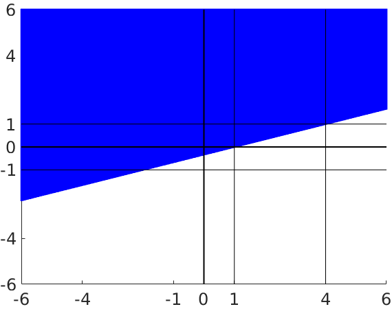
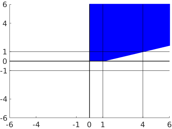
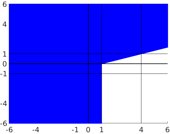
Let then the decision region of the first class can be computed recursively:
The outcome of each step is illustrated in Figure 8. One can clearly check that the decision region of the first class is given by
which is thus a disconnected set.
Overall, this counter-example shows that pyramidal structure of the network, at least under the other conditions of Theorem 3.10, is a necessary condition to get connected decision regions.
Does the result hold for ReLU activation function?
In the following, we show how to derive the decision regions of the network given in Equation (5).
