Continuum contact models for coupled adhesion and friction
Janine C. Mergel^a, Riad Sahli^b, Julien Scheibert^b, Roger A. Sauer^,a

^aGraduate School AICES, RWTH Aachen University, Templergraben 55, 52056 Aachen, Germany
^bLaboratoire de Tribologie et Dynamique des Systèmes LTDS UMR5513, Ecole Centrale de Lyon, ENISE, ENTPE, CNRS, F-69134, Ecully, France
Published in The Journal of Adhesion 95(12):1101–1133, 2019
Submitted on 21 February, 2018; accepted on 17 May, 2018

  Abstract: We develop two new continuum contact models for coupled adhesion and friction, and discuss them in the context of existing models proposed in the literature. Our new models are able to describe sliding friction even under tensile normal forces, which seems reasonable for certain adhesion mechanisms. In contrast, existing continuum models for combined adhesion and friction typically include sliding friction only if local contact stresses are compressive. Although such models work well for structures with sufficiently strong local compression, they fail to capture sliding friction for soft and compliant systems (like adhesive pads), for which the resistance to bending is low. This can be overcome with our new models. For further motivation, we additionally present experimental results for the onset of sliding of a smooth glass plate on a smooth elastomer cap under low normal loads. As shown, the findings from these experiments agree well with the results from our models. In this paper we focus on the motivation and derivation of our continuum contact models, and provide a corresponding literature survey. Their implementation in a nonlinear finite element framework as well as the algorithmic treatment of adhesion and friction will be discussed in future work.

Keywords: adhesion-controlled friction, tribology, dry adhesion, non-destructive testing, continuum contact mechanics, sliding friction

 

1 Introduction

This work is concerned with general contact models for adhesion mechanisms that are characterized by coupled adhesion and friction. Such mechanisms appear in both natural and technical applications; they also include the adhesive microstructures of many insects and lizards, which may resemble either soft adhesive pads (e.g. for flies and beetles) or rather stiff fibrils (e.g. for the gecko). In particular the gecko mechanism has several other remarkable properties like fast detachment, self-cleaning, and non-clumping [5]. To replicate the characteristics of bio-adhesives, various synthetic materials were developed [43, 44, 76, 10]. Like their natural counterparts, bio-inspired adhesives are often reusable and removable without leaving any residue. This makes them relevant for different medical applications; other possible applications include climbing robots, micro-electro-mechanical systems, and pick-and-place methods.

Initiated by the study of Autumn et al. [8], it is generally believed that bio-adhesion is mainly caused by van der Waals forces. Nevertheless, also other effects may have an influence, such as capillary [51] or electrostatic forces [53]. Within this paper, we mainly focus on dry adhesion due to van der Waals interactions. As experiments reveal, the function of bio- and bio-inspired adhesives further depends on friction (or “shear”) forces [6, 129]. Thus, the applications discussed so far do not only involve dry adhesion but also dry friction. Combined, adhesion and friction play an important role in various other systems; these include small frictional hairs at the legs of insects [63], the peeling of adhesive tapes [2], or elastomer spheres sliding on glass plates [101, 119, 25, 91].

Regarding bio-adhesive systems in general, experiments show that friction forces can occur even if the normal force is negative, i.e., tensile [6, 35, 129]. A similar observation can be made in experiments with chemically modified graphite surfaces [32]. Note that these findings usually refer to the total force in the system, while locally the contact stresses may vary between tension and compression within the same macroscopic contact area. This was demonstrated by Eason et al. [38], who used a tactile sensor to investigate the distribution of the normal stress underneath an attached gecko toe.

If an adhesive system has a large stiffness (or low compliance, respectively), its contact surface tends to be characterized by regions of tensile and regions of compressive contact forces. Then, the fraction of compressive and tensile areas is large compared to a more compliant system, which may justify the application of continuum models that capture friction only at the locally compressed parts of the contact area. However, for compliant, tape-like structures or soft adhesive pads (e.g. of insects, see [35]), the assumption of a high stiffness is not realistic. Existing continuum models for combined adhesion and friction include sliding friction only if the local contact stress is positive, i.e., compressive. Although they work well for systems with sufficiently strong (local) compression, they fail to capture sliding resistance for the cases described above.

We thus propose two general contact models for the analysis of physical problems that are characterized by coupled adhesion and friction. The first contact model is based on a constant sliding threshold within the contact area, which means the sliding shear is independent of the local distance of the contacting surfaces. This model turns out to be favorable for low normal loads, when friction is purely adhesion-controlled. The second model can be considered as a local version of Amontons’ law extended to adhesion. Both models are capable of capturing the frictional behavior for zero or negative (tensile) contact pressures. This approach is motivated by soft and compliant bio-adhesive pads, which are able to generate friction forces under tensile normal loads. We additionally present new experimental results for friction between a smooth elastomer sphere and a smooth glass plate. As shown, the findings from these experiments agree well with the results for the proposed models. Our contact models are formulated in the framework of large deformations, and apply to arbitrary geometries. For many applications this requires applying computational methods for analysis. An implementation of the proposed models in the framework of nonlinear finite element methods is addressed separately [70, 72].

To summarize, this work provides the following new aspects:

• A survey of existing models for dry adhesion and friction, which were proposed and applied in different fields of research;

• Experimental results for the onset of sliding of a glass plate on an elastomer sphere in the presence of low normal loads;

• Two new continuum models for coupled adhesion and friction of both biologic and bio-inspired adhesive systems; and

• A comparison of these models with the experiments.

The remainder of this paper is structured as follows. In Sect. 2 we discuss various mechanisms that may contribute to dry adhesion and friction, and review existing literature. We then present new experimental results in Sect. 3. In Sect. 4 we propose two models for adhesion and friction, and discuss their general behavior. Sect. 5 then provides a comparison of these models with the experiments, for which we consider the finite element formulation of [70, 72]. Sect. 6 finally concludes this paper.

2 Origin and modeling of adhesive friction

This section gives an overview of relevant experimental findings, theoretical models, and computational approaches that have been proposed in the past. In the following we will also refer to the terms sticking for static friction, and sliding for kinetic (or dynamic) friction, respectively.

2.1 Adhesive and non-adhesive friction

Like adhesion, dry friction may stem from (combinations of) different mechanisms at smaller length scales. This depends on the involved materials, surface properties, and the considered length scale. Mechanisms that contribute to friction are classified in [75] as follows: 1) adhesion; 2) deformation of asperities; 3) plastic deformation at the interface; 4) fracture; 5) interlocking; and 6) wear or contamination particles between the surfaces. Another possible mechanism is viscous dissipation in the material, e.g. for rubber or various tissues. Although sliding friction may be caused by a mixture of these mechanisms, in engineering applications it is often described by the well-known formula

$$F_{\mathrm{t}}=\mu\,F_{\mathrm{n}},\qquad F_{\mathrm{n}}>0,$$ (1)

where $\mu$ is the coefficient of sliding friction, which relates the normal and tangential forces, $F_{\mathrm{n}}$ and $F_{\mathrm{t}}$, to each other. Eq. 1 results from the following three laws, which were named after Guillaume Amontons and Charles de Coulomb:

1. The friction force is proportional to the applied normal load.  (Amontons’ $1\mathrm{st}$ law)

2. The friction force is independent of the apparent contact area.  (Amontons’ $2\mathrm{nd}$ law)

3. The friction force is independent of the sliding velocity.  (Coulomb’s law)

We will refer to relation 1 also as Coulomb-Amontons friction. The three laws stated above can be interpreted by introducing both an apparent (nominal) and a real (true) contact area, ${A_{\mathrm{real}}}$, and assuming that compressive contact occurs only between small microasperities. Such an approach goes back to [33, 16, 4], and explains the apparent contradiction in several experiments showing the friction force to be proportional to the contact area [102, 39]. In many applications, Eq. 1 describes frictional sliding of the system appropriately. Nevertheless, for considerably smooth surfaces or soft materials (such as polymers), Eq. 1 may not be valid anymore [82]. This was also shown for smooth elastomer contacts e.g. in [25, 91].

In a study of adhesion and friction of crystal layers, Derjaguin [33] used statistical analysis to derive a generalization of Amontons’ first law,

$$F_{\mathrm{t}}=\mu\,(F_{0}+F_{\mathrm{n}})=\mu\,{A_{\mathrm{real}}}\,(p_{0}+p_{\mathrm{n}}).$$ (2)

Here, $p_{\mathrm{n}}:=F_{\mathrm{n}}/{A_{\mathrm{real}}}$ is an averaged normal pressure, and $p_{0}:=F_{0}/{A_{\mathrm{real}}}$ is an adhesion parameter. After introducing a material-specific, critical shear stress $\tau_{0}:=\mu\,p_{0}$, Eq. 2 becomes

$$F_{\mathrm{t}}=\tau_{0}\,{A_{\mathrm{real}}}+\mu\,F_{\mathrm{n}}=\tau\,{A_{\mathrm{real}}},\qquad\tau:=\tau_{0}+\mu\,p_{\mathrm{n}}.$$ (3)

This will be referred to as extended Amontons’ law. According to Ruths et al. [88], Eq. 2 describes the friction force between dry surfaces that slide smoothly over each other in the presence of adhesion. For low normal loads, the first term in Eq. 3 predominates, which is called adhesion-controlled friction. For large normal loads, the second term (equivalent to Eq. 1) predominates, which is denoted pressure-controlled friction. The influence of both terms strongly depends on the specific application, and in particular on the smoothness, compliance, and adhesion of the contacting surfaces. This is demonstrated by the experimental results [50] shown in Fig. 1. For two molecularly smooth (and initially undamaged) mica cylinders sliding over each other, the friction force is directly proportional to the contact area; $F_{\mathrm{t}}=\tau_{0}\,{A_{\mathrm{real}}}$. This means that with increasing normal load, the friction force follows the triangles in the figure. At a sufficiently high normal load, damage occurs and forms wear particles at the interface. Afterwards, the normal load is decreased again. From that moment on, the friction force is proportional to the normal load according to Eq. 1, and not to the contact area anymore; see the filled circles in Fig. 1. As a comparison of Fig. 1(a) and Fig. 1(b) reveals, it depends on the specific parameters whether either adhesion- or pressure-controlled friction provide larger friction forces. The transition between both is further discussed in [11, 42, 54].

Removed for license reasons from arXiv preprint. See Fig. 4(a) in Ref. [50].

(a) Uncoated surfaces.

Removed for license reasons from arXiv preprint. See Fig. 4(b) in Ref. [50].

(b) Surfaces coated with calcium stearate.

Figure 1: Friction force and contact area measured for two mica cylinders sliding over each other in dry air. Dashed arrows indicate the transition between adhesion- and pressure-dependent friction.

Eq. 3 has been considered in various research fields, sometimes with a different terminology. It had already been discussed in a similar form before Derjaguin [33], also by Coulomb himself [42]. What he proposed was a fracture criterion for granular and brittle materials, known as the Mohr- or Navier-Coulomb criterion, respectively [29, 83]. Besides, Tabor [109] used Eq. 3 to derive a pressure-dependent friction model with an effective coefficient of sliding friction, $\hat{\mu}:=F_{\mathrm{t}}/F_{\mathrm{n}}=\tau_{0}/p_{\mathrm{n}}+\mu$. Extended Amontons’ law was further discussed in [19, 111, 126]. It also appeared in the context of microtribology [18, 12, 88], molecular dynamics simulations [42, 107, 73], and adhesive friction of bio- and bio-inspired systems [127, 49].

2.2 Existing modeling approaches

In the following, we give an overview of the most relevant models for dry adhesion and friction, with a special focus on continuum methods that are suitable for computational formulations. For a discussion of friction and tribology from a physical point of view, we refer to monographs [79, 14]. In addition, different aspects of nanotribology are addressed in book [13]. A recent review on modeling and simulation in tribology is given by Vakis et al. [116]. For an overview of computational models for adhesion, see also [94].

In order to model adhesion (and repulsion) due to van der Waals interactions, various continuum models have been developed based on the Lennard-Jones (LJ) potential

$$\phi(r)=\varepsilon\,{\Big{(}\frac{r_{0}}{r}\Big{)}}^{12}-2\,\varepsilon\,{\Big{(}\frac{r_{0}}{r}\Big{)}}^{6}.$$ (4)

Here, $\phi$ is the potential between two molecules separated by the distance $r$; it depends on the parameters $\varepsilon$ and $r_{0}$, which denote the depth of the potential well and the molecular equilibrium distance, respectively. In order to increase the efficiency of computational models based on Eq. 4, the interactions between two (in general arbitrarily shaped) bodies are often approximated by effective volumetric forces (with unit $\mathrm{N}/\mathrm{m}^{3}$) or effective surface tractions (with unit $\mathrm{N}/\mathrm{m}^{2}$). Such an approach is pursued in various computational formulations [98, 36, 100, 128, 40, 55].

In general, models based on the Lennard-Jones potential do not contain any contribution due to friction. For this reason, Deng et al. [32] additionally consider a constant tangential contact stress during sliding wherever the normal contact stress is compressive. This corresponds to the first term in Eq. 3, and thus shows similarities to one of our proposed models (Sect. 4.2.1). Apart from that, Jiang and Park [56] propose to extend the original Lennard-Jones potential by an additional “friction potential” in order to describe the friction properties of layered materials such as graphene. However, this approach is restricted to static friction.

Van der Waals forces can also be modeled by fitting traction-separation laws within a cohesive zone model; see e.g. [123, 78, 97, 99]. Although these papers use models that do not include tangential sliding, there also exist numerous cohesive zone models that additionally include sliding friction. In early works [114, 65], sliding friction according to Coulomb and Amontons was modeled subsequently after full tangential debonding. More recent cohesive zone models account for sliding friction also during partial separation [21, 87, 31, 108]. Besides, there exist several cohesive zone models including friction, which are based on representative interface or volume elements [1, 90, 89, 48].

In all of the cohesion models discussed so far, the damage caused by debonding is considered to be irreversible. This, however, is not realistic for van der Waals interactions. Schryve [106] and Cocou et al. [24] thus modified model [86] to capture partial recovering (“healing”) of the adhesive strength when the gap between the interfaces is closed again. Schryve applied this approach to investigate adhesion and friction between elastomer and glass.

Macroscopic adhesion and friction can also be modeled by statistical homogenization of the microscopic contact behavior [120]. Tworzydlo et al. [115], for instance, combined finite element simulations of small surface asperities with statistical analysis, mainly focusing on metallic surfaces. In that study adhesion was modeled with an integrated Lennard-Jones potential. Besides, there exists a recursive multiscale approach [121] to investigate contact of rubber and rough, rigid surfaces (like tire-road contact). This model captures van der Waals interactions by means of a fitted cohesive zone model, and restores adhesion fully when contact is re-established.

For completeness we also outline the most relevant models for non-adhesive friction. In a general continuum framework, sliding law 1 is usually stated in terms of the normal and tangential contact tractions, $t_{\mathrm{n}}$ and $\boldsymbol{t}_{\mathrm{t}}$,

$$\|\boldsymbol{t}_{\mathrm{t}}\|=\mu\,t_{\mathrm{n}},\qquad t_{\mathrm{n}}>0.$$ (5)

In many engineering applications it is sufficient to consider the coefficient of sliding friction, $\mu$, as a constant parameter for the material pair at the interface; see e.g. [23, 112, 3, 125]. Depending on the application, however, $\mu$ may be affected by the sliding velocity [47, 122], contact pressure [104], temperature [47], or microscopic time scales [113]. For an overview of approaches suitable for different kinds of materials see [120].

Note that both the friction and the cohesive zone models discussed above include sliding friction only under local compression. This means that after tangential debonding, frictionless sliding occurs if the normal contact stresses are tensile.

Next, we outline the most relevant small-deformation models for adhesion and friction. Regarding the frictionless adhesion of spheres, these include the well-known Johnson-Kendall-Roberts (JKR) [59] and Derjaguin-Muller-Toporov (DMT) [34] models, which apply to compliant and stiff materials, respectively. Both models were later combined in [68]. Although these models are restricted to small deformations and special contact geometries, they have been successfully applied to fit experimental data. In the experimental results shown in Fig. 1, for instance, the contact area agrees well with that predicted by the JKR theory. For adhesion-controlled friction, it is then possible to determine the frictional shear stress $\tau_{0}$ (a material-pair parameter) from sphere-plane contact as follows: 1) Predict the real contact area, ${A_{\mathrm{real}}}$, with the JKR theory by inserting Young’s modulus, the sphere radius, the applied normal load, and the interfacial adhesion energy; 2) measure the friction force, $F_{\mathrm{t}}$; and 3) combine both values using $F_{\mathrm{t}}=\tau_{0}\,{A_{\mathrm{real}}}$; see also Sect. 3. In Savkoor and Briggs [101], the JKR theory was extended further to incorporate the influence of tangential shearing. According to that model, for a fixed normal force, the contact area decreases with increasing tangential force. This agrees with the experimental findings presented therein. Related studies and important extensions include [57, 58, 119].

As mentioned in Sect. 2.1, friction may be explained by small asperities sliding over each other. Asperity-based friction models [17, 110] generally differ in the surface shape and the number of involved length scales; examples include periodic and wavy substrate, fractal surfaces, or stochastic profiles. Note that such approaches are also used in many of the papers outlined in Sect. 2.1, in particular to verify a linear relation between the real contact area and the normal force (see also [67, 80, 9]). Asperity-based models are not only used to investigate friction, but also adhesion. Multiasperity contact was combined both with the JKR [41] and DMT theory [22, 69]. Further extensions include [46, 85]. Like asperity-based friction models, models for rough surface adhesion can be based e.g. on a single layer of wavy asperities or on single- and multiscale fractal surfaces, respectively [77, 74]. For an overview see also [81].

Finally, there exists the analytical tape model [60] by Kendall, which was also extended numerous times to investigate directional peeling of thin strips or tapes. Some of these models also incorporate sliding friction. As experiments show, approaches of this type are suitable to accurately capture the peeling force of structures with small bending stiffness such as elastomer films [26], adhesive tape [28], and adhesive beetle pads [62]. These models are thus often applied to discuss the properties of bio-adhesive systems. For adhesive fibrils with finite bending stiffness, however, such models may underestimate the actual peel-off force considerably [93, 71].

3 Experimental results for sliding of a smooth elastomer sphere

We now present new experimental results for the onset of sliding of a smooth glass plate on a smooth polydimethylsiloxane (PDMS) sphere under low normal loads. Our experimental setup, inspired by Prevost et al. [84] and fully described in Sahli et al. [91], is illustrated in Fig. 2. As shown, the glass plate is attached to a double cantilever, which can deflect in the vertical direction (vertical stiffness $410\pm 20\,\mathrm{N}/\mathrm{m}$). The other end of the cantilever is mounted on a vertical translation stage (not shown in the figure), which allows the glass plate to be brought into and out of contact with the elastomer sphere. First contact is found by very slowly moving the double cantilever down and stopping as soon as the sphere snaps into adhesive contact with the glass. Going further down allows to obtain interfaces with increasing initial contact areas, ${A_{\mathrm{real}}}$. By analyzing the reflection images of the contact interface (see the method described in [91]), it is possible to monitor the evolution of ${A_{\mathrm{real}}}$ over time. The vertical displacement is then kept constant during the experiments.

Figure 2: Monitoring of the incipient sliding of a glass plate on an elastomer sphere: Sketch of the experimental setup.

Interestingly, once first contact has been formed, it is possible to move the double cantilever back up some distance without losing contact. This allows us to obtain interfaces in a global tensile state. Although our setup does not allow for measuring the resulting normal load directly, it is possible to estimate it from the initial contact area using the JKR theory [59]. This had been confirmed in an initial calibration on a dedicated device considering the same materials and contact geometry: Fitting the data by means of the JKR formula provided the values for Young’s modulus of our PDMS as well as the adhesion energy of our glass/PDMS interface (see Fig. 2).

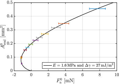
(a) Normal load vs. measured initial contact area.

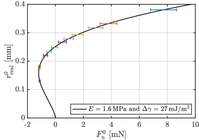
(b) Normal load vs. contact radius $r_{\mathrm{real}}^{0}=\sqrt{A_{\mathrm{real}}^{0}/\pi}$.

Figure 3: Initial contact of a glass plate on an elastomer sphere: Initial normal load $F_{\mathrm{n}}^{0}$ estimated from the measured initial contact area using the JKR theory and the material parameters in Fig. 2; each colored bar corresponds to a different experiment.

Fig. 3(a) shows the range of the initial normal forces $F_{\mathrm{n}}^{0}$ in dependence of the initial contact areas $A_{\mathrm{real}}^{0}$ measured in our experiments. Fig. 3(b) shows an alternative representation based on the corresponding contact radii. The horizontal bars in Fig. 3 indicate the possible range of values caused by uncertainties in the material parameters $E$ and $\Delta\gamma$ (Fig. 2). As these results imply, for some of the experiments the initial normal load is either close to zero or tensile.

The vertical translation stage at the end of the double cantilever is mounted on a motorized horizontal translation stage, enabling motion of the glass plate at a constant velocity $v=0.1\,\mathrm{m}\mathrm{m}/\mathrm{s}$. We measure the time evolution of the tangential load, $F_{\mathrm{t}}$, by means of a load sensor (resolution ca. $1\,\mathrm{m}\mathrm{N}$) as well as the time evolution of ${A_{\mathrm{real}}}$. A typical evolution of the contact area is shown in the snapshots of Fig. 4. As one can see, with increasing tangential loading, the area shrinks due to its left and right edges moving towards each other (with respect to the frame of the camera and the base of the sphere), while the left contact edge starts moving first.

Figure 4: Incipient sliding of a glass plate on an elastomer sphere: Snapshots of the contact area for an initial area of $0.27\,\mathrm{m}\mathrm{m}^{2}$, which is the upper yellow curve in Fig. 5(b); the sphere is fixed with respect to the frame of the camera, while the glass plate moves to the right; the driving velocity is $v=0.1\,\mathrm{m}\mathrm{m}/\mathrm{s}$; the bar shown in the first figure corresponds to a length of $0.25\,\mathrm{m}\mathrm{m}$.

Fig. 5(a) shows the tangential force, $F_{\mathrm{t}}$, as a function of time for different initial contact areas. Here, the origin of time, $t_{\mathrm{start}}$, is taken when the motor starts moving. For each curve, the typical behavior is the following: $F_{\mathrm{t}}$ increases, first almost linearly and then with a weakening slope, reaches its maximum (the static friction peak), and rapidly drops afterwards before entering a slow decay during macroscopic sliding. This slow decay, arising from a small residual angle between the glass plate and the horizontal, was negligible in [91]. Here, it is detectable because of the (about 20 times) smaller initial areas and the (about 8 times) stiffer cantilever.

The time evolution of the contact area ${A_{\mathrm{real}}}$ is plotted in Fig. 5(b). As shown also in [101, 119, 91], ${A_{\mathrm{real}}}$ decreases as the interface is progressively sheared. The rate of area decrease (i.e., the slope of the curve) significantly drops when the contact enters macroscopic sliding. The subsequent slow decrease of the area is the counterpart of the slow decrease of the friction force. Consistently with Waters and Guduru [119], contacts with the smallest initial areas (below about $0.1\,\mathrm{m}\mathrm{m}^{2}$) abruptly vanish upon shearing, without entering a macroscopic sliding regime. In contrast, the contacts with the highest initial areas (above about $0.19\,\mathrm{m}\mathrm{m}^{2}$) do not vanish during the time window shown in Figs. 5(a) and 5(b). For each experiment, this time window covers the time that is necessary to reach the static friction peak (squares in Fig. 5(a)), and to slide further by a distance that is equal to half times the width of the contact area at the static friction peak.

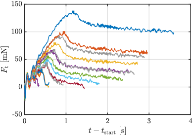
(a) Tangential force over time.

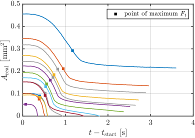
(b) Contact area over time.

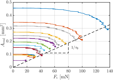
(c) Contact area as a function of the tangential force.

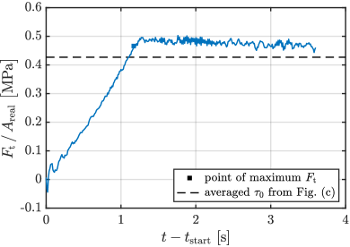
(d) $F_{\mathrm{t}}\,/\,{A_{\mathrm{real}}}$ over time for the largest initial contact.

Figure 5: Experimental results for the incipient sliding of a glass plate on an elastomer sphere: Friction force $F_{\mathrm{t}}$ and contact area ${A_{\mathrm{real}}}$ measured under low normal loads; each color corresponds to a different initial contact area (also shown in Fig. 3); the squares indicate the states with maximum $F_{\mathrm{t}}$; $t_{\mathrm{start}}$ is the instant when the motor starts to move at velocity $v=0.1\,\mathrm{m}\mathrm{m}/\mathrm{s}$.

Fig. 5(c) shows the dependency between the contact area and the tangential force in the incipient loading phase, before the friction peak is reached. As can be seen, at the onset of sliding (see the squares) the friction force and the contact area are, to a good approximation, proportional to each other. This is consistent with experimental results on identical smooth sphere/plane contacts [91], albeit for much larger contacts. It is also consistent with experiments on rough contacts involving soft materials (see e.g. [122, 30, 124, 91]).

Fig. 5(d) exemplarily shows the evolution of the ratio $F_{\mathrm{t}}\,/\,{A_{\mathrm{real}}}$ over time for the largest initial contact area (${A_{\mathrm{real}}}=0.46\,\mathrm{m}\mathrm{m}^{2}$, upper dark blue curve in Figs. 5(a) to 5(c)), for which both the small residual inclination of the glass plate and the resolution of the force sensor have lowest influence. This ratio corresponds to the average tangential traction within the contact area. As seen, it first increases almost linearly until the maximum friction force is reached. From then on, the ratio $F_{\mathrm{t}}\,/\,{A_{\mathrm{real}}}$ remains nearly constant. As these results demonstrate, considering a constant shear stress during sliding is a reasonable assumption when modeling friction of soft and smooth surfaces. This corresponds to adhesion-controlled friction, when $F_{\mathrm{t}}\approx\tau_{0}\,{A_{\mathrm{real}}}$ according to Eq. 3. For our experiments, we measure an average value of $\tau_{0}=0.43\pm 0.01\,\mathrm{M}\mathrm{P}\mathrm{a}$, which is also visualized in Fig. 5(c).

4 Models for adhesive friction

Before formulating adhesive friction between two arbitrary objects mathematically, we must first quantify the separation of their surfaces appropriately. To this end, we conceptually introduce variables for the distances in normal and tangential directions following classical contact formulations [64, 120]. Using a common notation in continuum mechanics (see e.g. [15]), we use uppercase letters for variables defined in the reference configuration of a body, and small letters for variables in the current configuration.

For a given point ${\boldsymbol{x}_{k}}$ on the contact surface of one of the two bodies $\mathcal{B}_{k}$, $k=1,2$, we first introduce its closest neighbor (or projection point), ${\boldsymbol{x}_{\ell}^{\mathrm{p}}}$, on the contact surface of the opposing body $\mathcal{B}_{\ell}$, $\ell=2,1$. At ${\boldsymbol{x}_{\ell}^{\mathrm{p}}}$, the outward unit normal vector of the surface is denoted $\boldsymbol{n}_{\mathrm{p}}$. Once these quantities are determined, we define a normal gap vector, ${\boldsymbol{g}_{\mathrm{n}}}$, as well as a (scalar) signed normal gap, ${g_{\mathrm{n}}}$, as

$${\boldsymbol{g}_{\mathrm{n}}}={\boldsymbol{x}_{k}}-{\boldsymbol{x}_{\ell}^{\mathrm{p}}},\qquad{g_{\mathrm{n}}}={\boldsymbol{g}_{\mathrm{n}}}\cdot\boldsymbol{n}_{\mathrm{p}}.$$ (6)

In addition, we conceptually introduce a vector for the tangential slip, ${\boldsymbol{g}_{\mathrm{t}}}$, which reduces to the scalar ${g_{\mathrm{t}}}$ for 2D problems. This quantity contains the magnitude and direction of the tangential displacement between the two surfaces. The normal and tangential gaps, ${g_{\mathrm{n}}}$ and ${\boldsymbol{g}_{\mathrm{t}}}$, as well as the normal vector, $\boldsymbol{n}_{\mathrm{p}}$, will be used to derive and illustrate our new contact models. Their computation is addressed e.g. in [95, 96], while the algorithmic treatment of combined adhesion and friction is discussed by Mergel et al. [70, 72].

4.1 Adhesive and repulsive contact

In order to describe general adhesion and repulsion between two bodies under large deformations, we consider the coarse-grained contact model (CGCM) [92, 98, 100]. This model is derived by first integrating the Lennard-Jones (LJ) potential from Eq. 4 over one of the two bodies (index $\ell$), assuming that its surface appears flat in the region affected by $\phi$ (typically a few nanometers). This yields a volumetric force (with unit $\mathrm{N}/\mathrm{m}^{3}$), which acts at each point within the other body (index $k$). In a second step, this body force is projected onto the surface of body $\mathcal{B}_{k}$ to obtain the contact traction (with unit $\mathrm{N}/\mathrm{m}^{2}$)

$${\boldsymbol{T}_{\mathrm{n},k}}=\frac{\theta_{k}}{J_{\ell}}\,T_{\mathrm{n}}({g_{\mathrm{n}}})\,\boldsymbol{n}_{\mathrm{p}},\qquad T_{\mathrm{n}}({g_{\mathrm{n}}})=\frac{{A_{\mathrm{H}}}}{2\pi r_{0}^{3}}\left[{\frac{1}{45}{\Big{(}\frac{r_{0}}{{g_{\mathrm{n}}}}\Big{)}}^{9}-\frac{1}{3}{\Big{(}\frac{r_{0}}{{g_{\mathrm{n}}}}\Big{)}}^{3}}\right].$$ (7)

Note that this contact law is stated in the undeformed reference configuration. As can be seen in Fig. 6, $T_{\mathrm{n}}$ can be split into a repulsive (power 9) and an attractive (power 3) term. In Eq. 7, the parameter ${A_{\mathrm{H}}}=2\pi^{2}\,\beta_{01}\,\beta_{02}\,\varepsilon\,r_{0}^{6}$ is the Hamaker constant [52], which contains the initial molecular densities $\beta_{0k}$ of the two bodies and the parameters $\varepsilon$ and $r_{0}$ of the Lennard-Jones potential. The scalar $J_{\ell}\geq 0$ denotes the volume change of the surrounding material during deformation. It corresponds to the determinant of the deformation gradient of the body $\mathcal{B}_{\ell}$ [100]. If this body is rigid, incompressible, or considerably stiffer than body $k$, one can assume that $J_{\ell}$ is either equal or close to one. The volume change can be related to the local surface stretch $J_{\mathrm{c}\ell}$ by using $J_{\ell}=J_{\mathrm{c}\ell}\cdot\lambda_{\ell}$, where $\lambda_{\ell}$ is the stretch along the thickness (perpendicular to the surface). Since the potential $\phi(r)$ rapidly decays to zero at large separations, it is reasonable to assume that within its effective range $\lambda_{\ell}\approx 1$, see also Sect. 2.3.2 of [95].

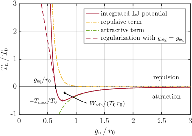
Figure 6: Contact traction in the model of Sauer and Wriggers [100] (“surface force formulation”) for frictionless adhesion and repulsion; $T_{0}={A_{\mathrm{H}}}\,/\,(2\pi r_{0}^{3})$.

Eq. 7 contains a scalar, $\theta_{k}$, that includes the current alignment of the two interacting surfaces as well as the volume change of body $\mathcal{B}_{k}$. Like $J_{\ell}$, $\theta_{k}$ requires the computation of the deformation in the vicinity of surface point $\boldsymbol{x}_{k}$. If both surfaces are parallel, and if the influence of the surface stretch of body $\mathcal{B}_{k}$ is negligible, one can set $\theta_{k}\approx 1$ [100]. In the following, we also assume that $\theta_{k}\approx 1$. An alternative approximation (similar to $J_{\ell}\approx J_{\mathrm{c}\ell}$) is proposed by Mergel in [70].

Before we proceed with the frictional part, let us define some characteristic parameters also shown in Fig. 6:

1. The equilibrium distance ${g_{\mathrm{eq}}}=r_{0}\,/\,\sqrt[6]{15}$ at which $T_{\mathrm{n}}({g_{\mathrm{eq}}})=0$ [93];

2. The work of adhesion per unit area for full separation, which is obtained by integrating $|T_{\mathrm{n}}({g_{\mathrm{n}}})|$ from ${g_{\mathrm{n}}}={g_{\mathrm{eq}}}$ to ${g_{\mathrm{n}}}=\infty$ [93],

   $$W_{\mathrm{adh}}=\frac{\sqrt[3]{15}\,{A_{\mathrm{H}}}}{16\pi r_{0}^{2}};$$ (8)

3. The location ${g_{\mathrm{max}}}$ of the maximum adhesive traction $T_{\mathrm{max}}$,

   $${g_{\mathrm{max}}}=\frac{r_{0}}{\sqrt[6]{5}},\qquad T_{\mathrm{max}}=|T_{\mathrm{n}}({g_{\mathrm{max}}})|=\frac{\sqrt{5}\,{A_{\mathrm{H}}}}{9\pi r_{0}^{3}}.$$ (9)

   Since $T_{\mathrm{n}}({g_{\mathrm{max}}})$ is negative (i.e., attractive), ${g_{\mathrm{max}}}$ is the global minimum of $T_{\mathrm{n}}$.

Furthermore, in a computational implementation, one may increase robustness by regularizing the normal traction for small normal gaps; see Apps. A and 6. This approach prevents ill-conditioning caused by the slope of $T_{\mathrm{n}}$ approaching minus infinity for decreasing ${g_{\mathrm{n}}}$.

4.2 Frictional contact

We now propose two new phenomenological models that combine adhesion and repulsion with sliding friction. To this end, we assume that the sliding resistance is equal to the threshold for static friction. This means that the tangential traction required to initiate the sliding process agrees with the traction in the final sliding state. This assumption is physically justified by experimental observations for both biological adhesives and rough elastomers, indicating that for such systems static friction is comparable to kinetic friction [7, 6, 129, 45, 84]. For the validity and restrictions of this assumption see also Sect. 4.4.

To shorten the notation, we now omit index $k$. Let $\boldsymbol{t}_{\mathrm{t}}({g_{\mathrm{n}}},{\boldsymbol{g}_{\mathrm{t}}})$ denote the tangential traction vector due to frictional sticking or sliding, which is a force per current area. $\boldsymbol{t}_{\mathrm{t}}$ depends on both the normal gap from Eq. 6 and the tangential slip ${\boldsymbol{g}_{\mathrm{t}}}$. We now assume that $\boldsymbol{t}_{\mathrm{t}}$ satisfies

$$\|\boldsymbol{t}_{\mathrm{t}}({g_{\mathrm{n}}},{\boldsymbol{g}_{\mathrm{t}}})\|\ \begin{cases}\ <\ t_{\mathrm{slide}}({g_{\mathrm{n}}})&\text{during\ sticking},\\ \ =\ t_{\mathrm{slide}}({g_{\mathrm{n}}})&\text{during\ sliding},\end{cases}$$ (10)

where $t_{\mathrm{slide}}({g_{\mathrm{n}}})\geq 0$ is a function that defines the sliding threshold. For $t_{\mathrm{slide}}$ we propose two different approaches in the next two subsections. Note that the classical Coulomb-Amontons law in Eq. 5 corresponds to $t_{\mathrm{slide}}:=\mu\,t_{\mathrm{n}}$ for $t_{\mathrm{n}}>0$.

4.2.1 Model DI: Distance-independent sliding friction in the contact area

The first proposed friction law is motivated by the experimental results discussed in Sect. 3. We simply assume that the sliding threshold is independent of the distance ${g_{\mathrm{n}}}$, i.e., constant within the current contact area. As a consequence, the resulting friction force is proportional to this area if the entire body is sliding. Let us first define some cutoff distance, ${g_{\mathrm{cut}}}$, up to which the surfaces are sufficiently close to each other in order to experience friction. After introducing a constant parameter $\tau_{\mathrm{D}\mathrm{I}}>0$ for the frictional shear strength, we define

$$t_{\mathrm{slide}}({g_{\mathrm{n}}})=\begin{cases}\tau_{\mathrm{D}\mathrm{I}},&{g_{\mathrm{n}}}\leq{g_{\mathrm{cut}}},\\ 0,&{g_{\mathrm{n}}}>{g_{\mathrm{cut}}}.\end{cases}$$ (11)

Since this function is discontinuous at ${g_{\mathrm{n}}}={g_{\mathrm{cut}}}$, we regularize it with the logistic function,

$$t_{\mathrm{slide}}({g_{\mathrm{n}}})=\frac{\tau_{\mathrm{D}\mathrm{I}}}{1+\mathrm{e}^{\,k_{\mathrm{D}\mathrm{I}}({g_{\mathrm{n}}}-{g_{\mathrm{cut}}})}},$$ (12)

where $k_{\mathrm{D}\mathrm{I}}>0$ (with unit $1/\mathrm{m}$) is a sufficiently large parameter. Both the original and the regularized models are illustrated in Fig. 7(a). Fig. 7(b) depicts the resulting friction law, i.e., the tangential traction-separation relation for arbitrary but fixed normal distances.

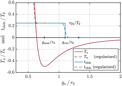
(a) Sliding threshold for varying ${g_{\mathrm{n}}}$.

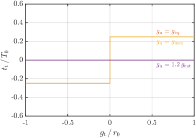
(b) Friction law in 2D for different but fixed ${g_{\mathrm{n}}}$.

Figure 7: Model DI: Constant sliding traction within the contact area defined by the cutoff distance ${g_{\mathrm{cut}}}$; $\tau_{\mathrm{D}\mathrm{I}}=0.5\,T_{\mathrm{max}}$, ${g_{\mathrm{cut}}}=1.1\,r_{0}$, and $T_{0}={A_{\mathrm{H}}}\,/\,(2\pi r_{0}^{3})$; the colored asterisks mark the normal gap values ${g_{\mathrm{eq}}}$ (where $T_{\mathrm{n}}=0$, orange), ${g_{\mathrm{max}}}$ (yellow), and $1.2\,{g_{\mathrm{cut}}}$ (purple).

Note that for the regularized model $t_{\mathrm{slide}}({g_{\mathrm{cut}}})=\tau_{\mathrm{D}\mathrm{I}}/2$. As seen in Fig. 7, for model DI both the value $\tau_{\mathrm{D}\mathrm{I}}$ and the cutoff distance ${g_{\mathrm{cut}}}$ can be chosen independently of the normal traction. Nevertheless, for the sake of comparison with the other model we introduce a coefficient that relates the constant $\tau_{\mathrm{D}\mathrm{I}}$ to the maximum adhesive traction $T_{\mathrm{max}}$, defined in Eq. 9, as

$$\mu_{\mathrm{D}\mathrm{I}}:=\frac{\tau_{\mathrm{D}\mathrm{I}}}{T_{\mathrm{max}}}.$$ (13)

The sliding threshold $\tau_{\mathrm{D}\mathrm{I}}$ is related to the actual contact surface (in the current configuration). This is motivated by the experiments from Sect. 3, for which the force is proportional to the current size of the contact area. If we defined the parameter $\tau_{\mathrm{D}\mathrm{I}}$ in the reference configuration instead, we would miss the change in the contact area. The differences between those two approaches are discussed in [70].

When recapitulating the unregularized version of model DI, one may recognize that Eq. 11 has some similarities to one of the earliest cohesive zone models, the Dugdale model [37]. In contrast to that model, however, we here define the sliding threshold for dynamic friction (instead of the normal stress during pure debonding). As mentioned also in Sect. 2.2, a similar approach is used in [32] to model sliding of graphene sheets. Therein, a constant stress during sliding is considered for those parts of the surfaces that are in compressive contact. This would correspond to the unregularized friction law 11 with ${g_{\mathrm{cut}}}={g_{\mathrm{eq}}}$. The current model is more general, because it can also be used to describe sliding resistance for tensile contact.

4.2.2 Model EA: Extended Amontons’ law in local form

The second proposed traction-separation law is inspired by extended Amontons’ law 3. Importantly, that law was originally formulated in terms of force resultants and average tractions. In our continuum formulation, however, the normal contact stress 7 can vary within the contact area between attraction and repulsion. To include a tangential resistance against sliding even for zero or negative normal pressures, we now propose a model that can be regarded as extended Amontons’ law in local form.

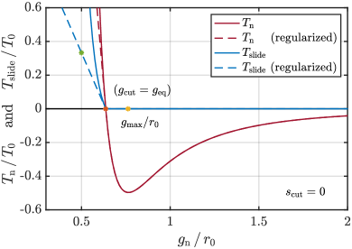
(a) Sliding threshold for varying ${g_{\mathrm{n}}}$; ${s_{\mathrm{cut}}}=0$.

(b) Friction law for different but fixed ${g_{\mathrm{n}}}$; ${s_{\mathrm{cut}}}=0$.

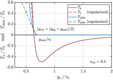
(c) Sliding threshold for varying ${g_{\mathrm{n}}}$; ${s_{\mathrm{cut}}}=0.5$.

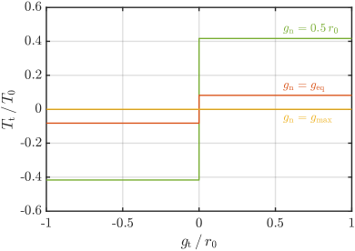
(d) Friction law for different but fixed ${g_{\mathrm{n}}}$; ${s_{\mathrm{cut}}}=0.5$.

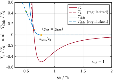
(e) Sliding threshold for varying ${g_{\mathrm{n}}}$; ${s_{\mathrm{cut}}}=1$.

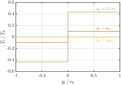
(f) Friction law for different but fixed ${g_{\mathrm{n}}}$; ${s_{\mathrm{cut}}}=1$.

Figure 8: Model EA: Extended Amontons’ law in local form illustrated for $\mu_{\mathrm{E}\mathrm{A}}=0.2$, $J_{\mathrm{c}\ell}\equiv 1$, and three different values of ${s_{\mathrm{cut}}}$; $T_{0}={A_{\mathrm{H}}}\,/\,(2\pi r_{0}^{3})$; the colored asterisks mark the normal gap values $0.5\,r_{0}$ (green), ${g_{\mathrm{eq}}}$ (where $T_{\mathrm{n}}=0$, orange), and ${g_{\mathrm{max}}}$ (yellow).

Let us first shift the traction $T_{\mathrm{n}}$ in Eq. 7 by a value smaller than or equal to the maximum adhesive traction, $T_{\mathrm{max}}$; see also Eqs. 9 and 6. To this end, we introduce a distance, ${g_{\mathrm{cut}}}$, which lies somewhere between the equilibrium distance, ${g_{\mathrm{eq}}}$, and the location ${g_{\mathrm{max}}}$ of $T_{\mathrm{max}}$:

$${g_{\mathrm{cut}}}={s_{\mathrm{cut}}}\,{g_{\mathrm{max}}}+(1-{s_{\mathrm{cut}}})\,{g_{\mathrm{eq}}},\qquad{s_{\mathrm{cut}}}\in[0,1].$$ (14)

As can be seen in Figs. 8(a) and 8(e), in this range $T_{\mathrm{n}}({g_{\mathrm{cut}}})$ is smaller than or equal to zero. We then consider a sliding threshold that is proportional to the shifted curve $T_{\mathrm{n}}({g_{\mathrm{n}}})+|T_{\mathrm{n}}({g_{\mathrm{cut}}})|$:

$$T_{\mathrm{slide}}({g_{\mathrm{n}}})=\begin{cases}\displaystyle\frac{\mu_{\mathrm{E}\mathrm{A}}}{J_{\mathrm{c}\ell}}\,\big{[}T_{\mathrm{n}}({g_{\mathrm{n}}})-T_{\mathrm{n}}({g_{\mathrm{cut}}})\big{]},&{g_{\mathrm{n}}}<{g_{\mathrm{cut}}},\\[0.86108pt] 0,&{g_{\mathrm{n}}}\geq{g_{\mathrm{cut}}}.\end{cases}$$ (15)

Note that in this case, the sliding threshold, $T_{\mathrm{slide}}$, directly depends on the normal traction, $T_{\mathrm{n}}$, which is defined in the reference configuration (Sect. 4.1).

Fig. 8 illustrates model EA for three different values of the parameter ${s_{\mathrm{cut}}}$. The left-hand side of the figure shows the dependence of the sliding traction, $T_{\mathrm{slide}}$, on the normal gap, ${g_{\mathrm{n}}}$; dashed lines indicate a regularized version according to App. A. If ${s_{\mathrm{cut}}}=0$ (Figs. 8(a) and 8(b)), tangential sliding occurs only for positive, i.e. compressive, normal tractions. This corresponds to classical Coulomb-Amontons friction (see Eq. 5) for non-adhesive contact. It is further used in many cohesive zone models (see Sect. 2.2) to include frictional sliding. If ${s_{\mathrm{cut}}}>0$, a tangential sliding resistance is present even for tensile normal tractions. Note that the curve for $T_{\mathrm{slide}}$ is smooth ($C^{1}$-continuous) only for ${s_{\mathrm{cut}}}=1$ (Fig. 8(e)); otherwise, a kink occurs at ${g_{\mathrm{n}}}={g_{\mathrm{cut}}}$, which requires special treatment in a computational implementation [70]. For the particular case ${s_{\mathrm{cut}}}=0$, this kink is exactly located at the equilibrium position, ${g_{\mathrm{eq}}}$.

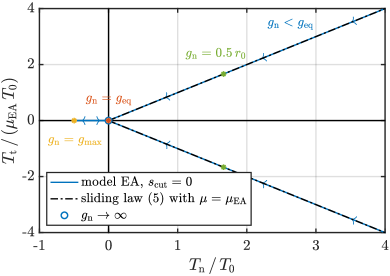
(a) Model EA with ${g_{\mathrm{cut}}}={g_{\mathrm{eq}}}$.

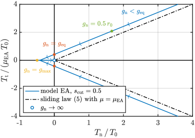
(b) Model EA with ${g_{\mathrm{cut}}}=({g_{\mathrm{eq}}}+{g_{\mathrm{max}}})/2$.

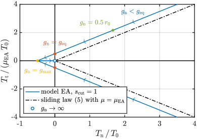
(c) Model EA with ${g_{\mathrm{cut}}}={g_{\mathrm{max}}}$.

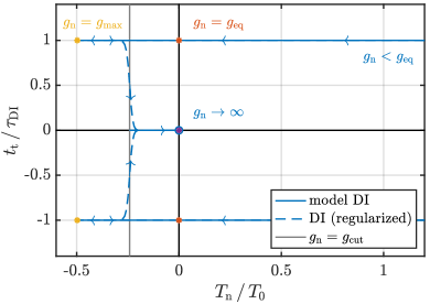
(d) Model DI.

Figure 9: Tangential traction during sliding vs. normal traction for (a) – (c) model EA with $J_{\mathrm{c}\ell}\equiv 1$ and (d) model DI; $T_{0}={A_{\mathrm{H}}}\,/\,(2\pi r_{0}^{3})$; the blue arrows indicate the sequence from ${g_{\mathrm{n}}}=0$ to ${g_{\mathrm{n}}}\to\infty$; for the colored asterisks see Figs. 7 and 8, respectively.

Fig. 9 depicts the (directed) tangential traction during sliding versus the normal traction, either for model EA and different values of ${s_{\mathrm{cut}}}$, or for model DI. As shown, for model EA this relation resembles a shifted version of the cone describing the classical friction law 5. In fact, up to ${g_{\mathrm{n}}}\leq{g_{\mathrm{cut}}}$, it corresponds to the Mohr-Coulomb model mentioned in Sect. 2.2. In model DI, the tangential traction, $t_{\mathrm{t}}$, is not a function of the normal traction, $t_{\mathrm{n}}$, anymore.

4.3 Continuum mechanical equations

For completeness this section outlines the governing equations for adhesive and frictional contact of two bodies. Under quasi-static conditions (for which inertial forces are neglected) the following equilibrium equations must be satisfied at each point ${\boldsymbol{x}_{k}}$ within the two bodies $\mathcal{B}_{k}$ $(k=1,\,2)$,

$$\mathrm{div}\,\mbox{\boldmath$\sigma$}_{k}+\boldsymbol{f}_{k}=\boldsymbol{0}.$$ (16)

Here, $\mbox{\boldmath$\sigma$}_{k}$ is the Cauchy stress tensor, and $\boldsymbol{f}_{k}$ denotes the vector of distributed volumetric forces. The bodies must further satisfy the contact condition

$$\mbox{\boldmath$\sigma$}_{k}\,\boldsymbol{n}_{k}={\boldsymbol{t}_{\mathrm{n},k}}-{\boldsymbol{t}_{\mathrm{t},k}}$$ (17)

on the contact surface $\partial_{\mathrm{c}}\mathcal{B}_{k}$, as well as conditions at the Dirichlet boundaries $\partial_{\boldsymbol{u}}\mathcal{B}_{k}$ (where displacements $\bar{\boldsymbol{u}}_{k}$ are prescribed)

$$\boldsymbol{x}_{k}-\boldsymbol{X}_{k}=\bar{\boldsymbol{u}}_{k},$$ (18)

and at the Neumann boundaries $\partial_{\boldsymbol{t}}\mathcal{B}_{k}$ (where surface tractions $\bar{\boldsymbol{t}}_{k}$ are applied),

$$\mbox{\boldmath$\sigma$}_{k}\,\boldsymbol{n}_{k}=\bar{\boldsymbol{t}}_{k}.$$ (19)

In Eqs. 17 and 19, the unit vector $\boldsymbol{n}_{k}$ denotes the current surface normal at point ${\boldsymbol{x}_{k}}$. Eq. 17 further contains the normal and tangential tractions defined through our contact models; note that here the sign convention of Laursen [64] is used. Eqs. 16 to 19 represent the strong form of the general contact and boundary value problem, expressed in the current configurations of the bodies. Since the analytical solution of these equations is possible only for very special cases (and mainly restricted to small deformations), for general conditions involving arbitrary geometries and large deformations, a computational solution technique is required. For this reason, [70, 72] provide a computational implementation of our models into a nonlinear finite element formulation, and also discuss the algorithmic treatment of friction under large deformations.

4.4 General comments, validity, and restrictions

Like any other model, our models have limitations. We address those in the following.

In Eq. 10 we assume that the static friction threshold coincides with the resistance for kinetic friction. As mentioned at the beginning of Sect. 4.2, this assumption agrees well with experimental observations for bio-adhesive systems and rough elastomers. Nevertheless, these observations refer to the globally measured force resultant instead of the local traction at the contact zone. It remains to be discussed further whether static and kinetic friction coincide because of the material itself, or whether this is caused by a split of the effective contact area into a large number of small areas. The influence of such a split on both static friction and stick-slip motion is addressed in [117, 118, 66]. Regarding bio-inspired adhesives, it may be arguable whether the assumption of equal static and kinetic friction is valid for all kinds of materials. See, for instance, the experimental results [117] obtained for a microstructured polyvinylsiloxane (PVS) surface sliding on glass. If required, our model could be extended to account for differing parameters for static and kinetic friction as well.

In our model we consider dry (i.e., non-lubricated) adhesion and friction. We hence omit the influence of any secretion that may cover the adhesive device, as observed for many beetles and other insects. In fact, experimental studies on insect pads show that the depletion of such secretion (caused e.g. by sliding or by repeating detachment) affects both their frictional resistance [35, 20] and (although less strongly) their adhesion [61]. Nevertheless, if the amount of sliding is sufficiently small, one can assume that the frictional resistance does not change considerably.

As shown in Sects. 1 and 3, there exist several applications for which van der Waals forces may affect the macroscopic behavior even at larger scales (micrometers or millimeters). For increasing length scales, a direct computational implementation of adhesion models based on the Lennard-Jones potential, such as the CGCM model (Sect. 4.1) and friction model EA, can become very inefficient, because they require nanoscale finite element resolution. For this reason, it would be very promising to develop an effective adhesion model that is regularized by the compliance of the surrounding material. One approach in this direction has been developed in the context of adhesive joints under small deformations [105]. Another possibility, which is pursued in [70, 72] and also here, is to calibrate the parameters in Sect. 4.1 (like ${A_{\mathrm{H}}}$, $T_{\mathrm{max}}$, or $W_{\mathrm{adh}}$) such that they match with experimental data. The curve 7 is then regularized by an automatic increase of the length parameter $r_{0}$. As a consequence, the model does not require nanoscale resolution anymore. When adjusting these parameters it is important to distinguish between the nominal (or apparent) contact area and the true contact area due to very small asperities, which interact at the contact surface; see also the discussion in Sect. 2.1. For the CGCM of Sect. 4.1 the normal contact stress is integrated over an apparent, nominally flat contact area. Thus, simply inserting the material constant ${A_{\mathrm{H}}}$ for the considered pair of materials would overestimate the real strength of adhesion by several orders of magnitude. This can be overcome by directly inserting effectively measured values as described before. Note that in general, the ratio between the true and the nominal contact areas may depend on the contact pressure, as discussed in Sect. 5.2.4 of [120] from a computational point of view.

5 Qualitative comparison between model and experiment

We now apply the proposed two models to study adhesive friction between a soft cylindrical cap and a rigid substrate, see Fig. 10(a). To this end, we use the finite element implementation derived in [70, 72].

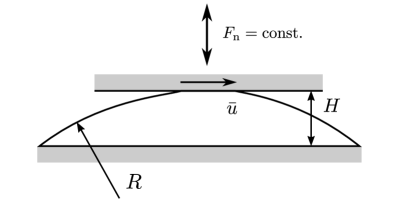
(a) Problem setup.

(b) Sliding under zero normal load.

Figure 10: Adhesive friction of a soft cap: (a) Setup; (b) stress distribution during sliding for zero preload and model DI (${g_{\mathrm{cut}}}={g_{\mathrm{max}}}$, $\mu_{\mathrm{D}\mathrm{I}}=1$); the colors show the first invariant of the Cauchy stress in units of $E$.

We consider this example as a preliminary study to investigate the qualitative behavior of our models, and to show that it agrees with the experimental behavior presented in Sect. 3. For length scale reasons related to the computational adhesion model [100] (addressed in detail in Sect. 4.4 already), a quantitative comparison is not possible at this stage. Therefore, the cap in the example is 2D and smaller than that in Sect. 3. Also, slightly different material parameters (Tab. 1) and smaller friction values are used. A 2D plane strain, nonlinear finite element formulation based on a Neo-Hooke material model is used to simulate the example. For further details see [70]. All results shown here are normalized by Young’s modulus, $E$, an arbitrary out-of-plane thickness (or width), $W$, and a unit length, $L_{0}$ (see Tab. 1).

$E$	$\nu$	$T_{\mathrm{max}}$	$W_{\mathrm{adh}}$	$R$	H	$L_{0}$
$2\,\mathrm{M}\mathrm{P}\mathrm{a}$	$0.4$	$0.33\,\mathrm{M}\mathrm{P}\mathrm{a}$	$0.027\,\mathrm{J}/\mathrm{m}^{2}$	$47.1\,L_{0}$	$10\,L_{0}$	$1\,\mu\mathrm{m}$

Table 1: Adhesive friction of a soft cap: Parameters.

As illustrated in Fig. 10(a), we first apply a fixed normal force to the rigid substrate, and then slide it horizontally while keeping the lower boundary of the cap fixed. As a special case we investigate the sliding behavior also under zero load, for which the attractive and repulsive stresses in the contact area equilibrate each other. The finite element mesh of the cap consists of 42,300 Q1N2.1 elements [27]. Fig. 10(b) shows the stress distribution of the cap during sliding under zero load.

Although keeping the normal load constant during sliding is not strictly identical to the boundary conditions in our experiment, in the latter the normal load is expected to remain reasonably close to its initial value predicted from the JKR theory (Fig. 3): Since the end of the double cantilever (see Sect. 3) is kept vertically fixed, the vertical position of the glass plate, and thus the normal load, can change only due to a vertical dilatancy of the elastomer sphere caused by horizontal shear. According to Scheibert et al. [103] (see the introduction and references therein), however, in our case of a rigid body (glass plate) in contact with an incompressible half-space (thick elastomer with a Poisson’s ratio of approx. $0.5$), the coupling between the normal displacement and any induced tangential stresses is expected to be negligible. For a qualitative comparison as it is performed here, it is expected that the slight differences in the boundary conditions do not affect our general observations and conclusions.

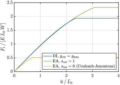
(a) Friction force under compression, $F_{\mathrm{n}}^{*}=-0.288$.

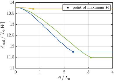
(b) Contact area under compression, $F_{\mathrm{n}}^{*}=-0.288$.

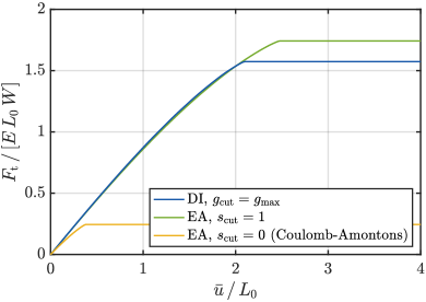
(c) Friction force under zero load, $F_{\mathrm{n}}^{*}=0$.

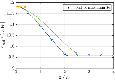
(d) Contact area under zero load, $F_{\mathrm{n}}^{*}=0$.

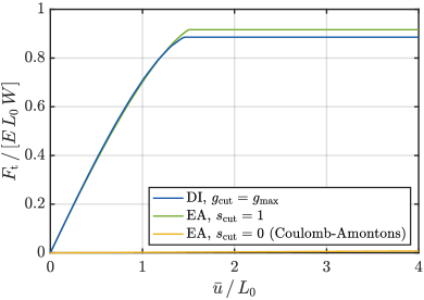
(e) Friction force under tension, $F_{\mathrm{n}}^{*}=0.288$.

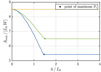
(f) Contact area under tension, $F_{\mathrm{n}}^{*}=0.288$.

Figure 11: Adhesive friction of a soft cap: Friction force and contact area for sliding under a constant preload ($\mu_{\mathrm{E}\mathrm{A}}=\mu_{\mathrm{D}\mathrm{I}}=1$); the squares indicate the onset of full sliding; the dots mark the configurations of Fig. 13; $F_{\mathrm{n}}^{*}=F_{\mathrm{n}}\,/\,\big{[}E\,L_{0}\,W\big{]}$ denotes the normalized preload.

Fig. 11 shows both the friction force and the contact area for different loads. Here we use models DI with ${g_{\mathrm{cut}}}={g_{\mathrm{max}}}$, EA with ${s_{\mathrm{cut}}}=1$, and EA with ${s_{\mathrm{cut}}}=0$ (Coulomb-Amontons friction, see also Eq. 5). Before full sliding, the qualitative behavior of all models is close to our experimental results in Figs. 5(a) and 5(b). For classical Coulomb-Amontons friction, however, the sliding force is considerably lower than for the other models, because the compressed area is much smaller than the total contact area. When the entire contact surface is sliding, both the force and the area remain constant for the numerical models. In contrast, in the experiments, the tangential force drops over a finite time scale before entering a rather steady sliding regime. These differences are most likely caused by the viscous behavior of polydimethylsiloxane. It thus makes sense to later consider a viscoelastic material model.

Fig. 12 (like Fig. 5(c)) shows the contact area versus the tangential force up to the point of full sliding. The classical law by Coulomb and Amontons (model EA for ${s_{\mathrm{cut}}}=0$) obviously fails to capture the qualitative behavior observed in the experiments. In contrast, the differences to the experimental results are smaller for model EA with ${s_{\mathrm{cut}}}=1$, but they are still considerable. Model DI, on the other hand, agrees very well with the experiments.

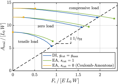
Figure 12: Adhesive friction of a soft cap: Contact area as a function of the tangential force for the onset of sliding under different preloads ($\mu_{\mathrm{E}\mathrm{A}}=\mu_{\mathrm{D}\mathrm{I}}=1$); $\tau_{\mathrm{D}\mathrm{I}}=\mu_{\mathrm{D}\mathrm{I}}\,T_{\mathrm{max}}$; see also Fig. 5(c).

Figure 13: Adhesive friction of a soft cap: Evolution of the contact interface during sliding for model DI and zero normal load (see the dots in Fig. 11(d)); the vertical axis is stretched by the factor $\approx 3.93$; the configuration at zero tangential displacement ($\bar{u}=0$) as well as its contour are shown in orange; the other colors show the first invariant of the Cauchy stress in units of $E$.

Finally, Fig. 13 shows (a vertically stretched view of) the contact interface for model DI. As a comparison with the first four snapshots of Fig. 4 implies, model DI appropriately captures the qualitative behavior of the contact edges before the friction force reaches its static friction peak (see the squares in Figs. 5 and 11(d)). Beforehand, mainly the left contact edge moves rightward with respect to the base of the sphere. The subsequent leftward motion of the right edge (observed in the experiments, see the last three snapshots in Fig. 4) is not seen in the numerical results, which is also likely caused by the viscosity of the material. In summary, combining model DI with a viscous material model seems to be a promising approach to model sliding of smooth rubber spheres on glass.

6 Conclusion

In this paper, we present two new continuum contact models for coupled adhesion and friction that are suitable for soft systems like biological and bio-inspired adhesives. These two models are based on a 3D continuum adhesion formulation [100], which is suitable to describe large deformations and large sliding motions. As a motivation, we first provide a review of existing experimental studies, theoretical investigations, and modeling approaches for dry adhesion and friction. We also present new experimental results for a smooth glass plate sliding on a smooth PDMS cap under low normal loads. Our findings indicate that the classical law by Coulomb and Amontons (with a linear dependence between the normal and tangential loads) is not applicable for strong adhesion or small roughnesses. In this case the friction force is also affected by an additional adhesion term. For some applications, this additional term dominates, and the sliding resistance is described by a constant, material-dependent frictional shear strength multiplied with the real contact area. Our two continuum models can generate sliding friction even when the normal pressure is zero or negative (i.e., tensile). This is useful because soft bio-adhesive pads are observed to generate non-negligible sliding forces under zero normal load. The proposed models contain the law of Coulomb and Amontons as a special case. As demonstrated in [70, 72], for certain applications both models show very similar behavior.

This paper focuses on the motivation and derivation of our new contact models. Both their implementation in terms of a nonlinear finite element framework and the algorithmic treatment of adhesive friction are discussed separately [70, 72]. In [70] the model is further incorporated into a beam contact model [99] for adhesive fibrils.

As an example we here investigate adhesive friction of a soft cap and a rigid substrate, and show that the model behavior is in qualitative agreement to the experiments. Our work is also a first important step towards a better understanding and modeling of biologic adhesives: As shown in [70], model DI is also suitable to qualitatively describe the characteristics of friction devices in stick insects. It would thus be very promising to perform additional experiments on those, and to calibrate our friction models accordingly.

In future work, several extensions should be developed to overcome the restrictions mentioned in Sect. 4.4, in particular the restriction to small length scales that is inherent to numerical van der Waals-based contact formulations. A contact homogenization technique should be able to overcome this. The current comparison between model and experiment is qualitative. With a refined model, it will be possible to conduct quantitative comparisons, which will require further experiments with both biologic and bio-inspired adhesives. It would also be interesting to apply model EA to problems in which both adhesion- and pressure-controlled friction play a role.

Appendix A Regularization for small normal distances

To avoid ill-conditioning, it is possible to regularize the contact stress for small normal gaps, ${g_{\mathrm{n}}}\to 0$, e.g. by means of linear extrapolation. To this end, we introduce $T_{\mathrm{n}}({g_{\mathrm{n}}})\approx T_{\mathrm{n}}^{\mathrm{reg}}({g_{\mathrm{n}}})$,

$$T_{\mathrm{n}}^{\mathrm{reg}}({g_{\mathrm{n}}})=\begin{cases}T_{\mathrm{n}}({g_{\mathrm{n}}}),&{g_{\mathrm{n}}}\geq g_{\mathrm{reg}},\\ T_{\mathrm{n}}(g_{\mathrm{reg}})+T_{\mathrm{n}}^{\prime}(g_{\mathrm{reg}})\,({g_{\mathrm{n}}}-g_{\mathrm{reg}}),&{g_{\mathrm{n}}}<g_{\mathrm{reg}};\end{cases}$$ (20)

see also Fig. 6. $T_{\mathrm{n}}^{\prime}$ denotes the derivative of $T_{\mathrm{n}}$ with respect to ${g_{\mathrm{n}}}$. It is reasonable to choose a regularization distance of $g_{\mathrm{reg}}\approx{g_{\mathrm{eq}}}$, where ${g_{\mathrm{eq}}}$ is the equilibrium distance. For $g_{\mathrm{reg}}\leq{g_{\mathrm{eq}}}$, the attractive part of the curve in Fig. 6 remains unaffected; if $g_{\mathrm{reg}}>{g_{\mathrm{eq}}}$, one also modifies the work of adhesion, $W_{\mathrm{adh}}$, in Eq. 8, and shifts ${g_{\mathrm{eq}}}$ to another position.

References

- [1] G. Alfano and E. Sacco. Combining interface damage and friction in a cohesive-zone model. Int. J. Numer. Methods Eng., 68(5):542–582, 2006.
- [2] N. Amouroux, J. Petit, and L. Léger. Role of interfacial resistance to shear stress on adhesive peel strength. Langmuir, 17:6510–6517, 2001.
- [3] D. S. Amundsen, J. K. Trømborg, K. Thøgersen, E. Katzav, A. Malthe-Sørenssen, and J. Scheibert. Steady-state propagation speed of rupture fronts along one-dimensional frictional interfaces. Phys. Rev. E, 92:032406, 2015.
- [4] J. F. Archard. Elastic deformation and the laws of friction. Proc. R. Soc. London A, 243:190–205, 1957.
- [5] K. Autumn. Properties, principles, and parameters of the gecko adhesive system. In A. M. Smith and J. A. Callow, editors, Biological Adhesives, pages 225–256. Springer, Berlin Heidelberg, 2006.
- [6] K. Autumn, A. Dittmore, D. Santos, M. Spenko, and M. Cutkosky. Frictional adhesion: A new angle on gecko attachment. J. Exp. Biol., 209:3569–3579, 2006.
- [7] K. Autumn, Y. A. Liang, S. T. Hsieh, W. Zesch, W. P. Chan, T. W. Kenny, R. Fearing, and R. J. Full. Adhesive force of a single gecko foot-hair. Nature, 405:681–685, 2000.
- [8] K. Autumn, M. Sitti, Y. A. Liang, A. M. Peattie, W. R. Hansen, S. Sponberg, T. W. Kenny, R. Fearing, J. N. Israelachvili, and R. J. Full. Evidence for van der Waals adhesion in gecko setae. Proc. Natl. Acad. Sci. U.S.A., 99(19):12252–12256, 2002.
- [9] J. R. Barber. Multiscale surfaces and Amontons’ law of friction. Tribol. Lett., 49:539–543, 2013.
- [10] M. D. Bartlett, A. B. Croll, D. R. King, B. M. Paret, D. J. Irschick, and A. J. Crosby. Looking beyond fibrillar features to scale gecko-like adhesion. Adv. Mater., 24:1078–1083, 2012.
- [11] A. Berman, C. Drummond, and J. Israelachvili. Amontons’ law at the molecular level. Tribol. Lett., 4:95–101, 1998.
- [12] A. Berman, S. Steinberg, S. Campbell, A. Ulman, and J. Israelachvili. Controlled microtribology of a metal oxide surface. Tribol. Lett., 4:43–48, 1998.
- [13] B. Bhushan, editor. Nanotribology and Nanomechanics. Springer, Berlin Heidelberg, 2005.
- [14] B. Bhushan. Introduction to Tribology. Wiley, New York, edition, 2013.
- [15] J. Bonet and R. D. Wood. Nonlinear Continuum Mechanics for Finite Element Analysis. Cambridge University Press, 1997.
- [16] F. P. Bowden and D. Tabor. The area of contact between stationary and between moving surfaces. Proc. R. Soc. London A, 169:391–413, 1939.
- [17] O. M. Braun and M. Peyrard. Modeling friction on a mesoscale: Master equation for the earthquakelike model. Phys. Rev. Lett., 100:125501, 2008.
- [18] B. J. Briscoe and S. L. Kremnitzer. A study of the friction and adhesion of polyethylene-terephthalate monofilaments. J. Phys. D: Appl. Phys., 12:505–517, 1979.
- [19] B. J. Briscoe and D. Tabor. Friction and wear of polymers: the role of mechanical properties. Br. Polym. J., 10:74–78, 1978.
- [20] J. M. R. Bullock, P. Drechsler, and W. Federle. Comparison of smooth and hairy attachment pads in insects: friction, adhesion and mechanisms for direction-dependence. J. Exp. Biol., 211:3333–3343, 2008.
- [21] J. L. Chaboche, R. Girard, and A. Schaff. Numerical analysis of composite systems by using interphase/interface models. Comput. Mech., 20:3–11, 1997.
- [22] W. R. Chang, I. Etsion, and D. B. Bogy. Adhesion model for metallic rough surfaces. J. Tribol., 110:50–55, 1988.
- [23] M. Ciavarella. The generalized Cattaneo partial slip plane contact problem. II — Examples. Int. J. Solids Struct., 35(18):2363–2378, 1998.
- [24] M. Cocou, M. Schryve, and M. Raous. A dynamic unilateral contact problem with adhesion and friction in viscoelasticity. Z. angew. Math. Phys. (ZAMP), 61:721–743, 2010.
- [25] C. Cohen, F. Restagno, C. Poulard, and L. Léger. Incidence of the molecular organization on friction at soft polymer interfaces. Soft Matter, 7:8535–8541, 2011.
- [26] R. R. Collino, N. R. Philips, M. N. Rossol, R. M. McMeeking, and M. R. Begley. Detachment of compliant films adhered to stiff substrates via van der Waals interactions: role of frictional sliding during peeling. J. R. Soc. Interface, 11:20140453, 2014.
- [27] C. J. Corbett and R. A. Sauer. NURBS-enriched contact finite elements. Comput. Methods Appl. Mech. Eng., 275:55–75, 2014.
- [28] M.-J. Dalbe, R. Villey, M. Ciccotti, S. Santucci, P.-P. Cortet, and L. Vanel. Inertial and stick-slip regimes of unstable adhesive tape peeling. Soft Matter, 12:4537–4548, 2016.
- [29] F. V. de Blasio. Introduction to the Physics of Landslides. Lecture Notes on the Dynamics of Mass Wasting. Springer, 2011.
- [30] E. Degrandi-Contraires, C. Poulard, F. Restagno, and L. Léger. Sliding friction at soft micropatterned elastomer interfaces. Faraday Discuss., 156:255–265, 2012.
- [31] G. Del Piero and M. Raous. A unified model for adhesive interfaces with damage, viscosity, and friction. Eur. J. Mech. A/Solids, 29:496–507, 2010.
- [32] Z. Deng, A. Smolyanitsky, Q. Li, X.-Q. Feng, and R. J. Cannara. Adhesion-dependent negative friction coefficient on chemically modified graphite at the nanoscale. Nat. Mater., 11:1032–1037, 2012.
- [33] B. Derjaguin. Molekulartheorie der äußeren Reibung. Z. Phys., 88:661–675, 1934.
- [34] B. V. Derjaguin, V. M. Muller, and Y. P. Toporov. Effect of contact deformations on the adhesion of particles. J. Colloid Interface Sci., 53(2):314–325, 1975.
- [35] P. Drechsler and W. Federle. Biomechanics of smooth adhesive pads in insects: influence of tarsal secretion on attachment performance. J. Comp. Physiol. A, 192:1213–1222, 2006.
- [36] Y. Du, L. Chen, N. E. McGruer, G. G. Adams, and I. Etsion. A finite element model of loading and unloading of an asperity contact with adhesion and plasticity. J. Colloid Interface Sci., 312:522–528, 2007.
- [37] D. S. Dugdale. Yielding of steel sheets containing slits. J. Mech. Phys. Solids, 8:100–104, 1960.
- [38] E. V. Eason, E. W. Hawkes, M. Windheim, D. L. Christensen, T. Libby, and M. R. Cutkosky. Stress distribution and contact area measurements of a gecko toe using a high-resolution tactile sensor. Bioinspir. Biomim., 10:016013, 2015.
- [39] M. Enachescu, R. J. A. van den Oetelaar, R. W. Carpick, D. F. Ogletree, C. F. J. Flipse, and M. Salmeron. Observation of proportionality between friction and contact area at the nanometer scale. Tribol. Lett., 7:73–78, 1999.
- [40] H. Fan and S. Li. A three-dimensional surface stress tensor formulation for simulation of adhesive contact in finite deformation. Int. J. Numer. Methods Eng., 107(3):252–270, 2015.
- [41] K. N. G. Fuller and D. Tabor. The effect of surface roughness on the adhesion of elastic solids. Proc. R. Soc. London A, 345:327–342, 1975.
- [42] J. Gao, W. D. Luedtke, D. Gourdon, M. Ruths, J. N. Israelachvili, and U. Landman. Frictional forces and Amontons’ law: From the molecular to the macroscopic scale. J. Phys. Chem. B, 108:3410–3425, 2004.
- [43] A. K. Geim, S. V. Dubonos, I. V. Grigorieva, K. S. Novoselov, A. A. Zhukov, and S. Y. Shapoval. Microfabricated adhesive mimicking gecko foot-hair. Nat. Mater., 2:461–463, 2003.
- [44] S. Gorb, M. Varenberg, A. Peressadko, and J. Tuma. Biomimetic mushroom-shaped fibrillar adhesive microstructure. J. R. Soc. Interface, 4:271–275, 2007.
- [45] N. Gravish, M. Wilkinson, S. Sponberg, A. Parness, N. Esparza, D. Soto, T. Yamaguchi, M. Broide, M. Cutkosky, C. Creton, and K. Autumn. Rate-dependent frictional adhesion in natural and synthetic gecko setae. J. R. Soc. Interface, 7:259–269, 2010.
- [46] J. A. Greenwood and K. L. Johnson. The mechanics of adhesion of viscoelastic solids. Phil. Mag. A, 43(3):697–711, 1981.
- [47] K. A. Grosch. The relation between the friction and visco-elastic properties of rubber. Proc. R. Soc. A, 274:21–39, 1963.
- [48] I. Guiamatsia and G. D. Nguyen. A thermodynamics-based cohesive model for interface debonding and friction. Int. J. Solids Struct., 51:647–659, 2014.
- [49] G. C. Hill, D. R. Soto, A. M. Peattie, R. J. Full, and T. W. Kenny. Orientation angle and the adhesion of single gecko setae. J. R. Soc. Interface, 8:926–933, 2011.
- [50] A. M. Homola, J. N. Israelachvili, P. M. McGuiggan, and M. L. Gee. Fundamental experimental studies in tribology: The transition from “interfacial” friction of undamaged molecularly smooth surfaces to “normal” friction with wear. Wear, 136:65–83, 1990.
- [51] G. Huber, H. Mantz, R. Spolenak, K. Mecke, K. Jacobs, S. N. Gorb, and E. Arzt. Evidence for capillarity contributions to gecko adhesion from single spatula nanomechanical measurements. Proc. Natl. Acad. Sci. U.S.A., 102(45):16293–16296, 2005.
- [52] J. N. Israelachvili. Intermolecular and Surface Forces. Academic Press, edition, 2011.
- [53] H. Izadi, K. M. E. Stewart, and A. Penlidis. Role of contact electrification and electrostatic interactions in gecko adhesion. J. R. Soc. Interface, 11:20140371, 2014.
- [54] A. Jagota and C.-Y. Hui. Adhesion, friction, and compliance of bio-mimetic and bio-inspired structured interfaces. Mater. Sci. Eng. R, 72:253–292, 2011.
- [55] U. B. Jayadeep, M. S. Bobji, and C. S. Jog. A body-force formulation for analyzing adhesive interactions with special considerations for handling symmetry. Finite Elem. Anal. Des., 117–118:1–10, 2016.
- [56] J.-W. Jiang and H. S. Park. A Gaussian treatment for the friction issue of Lennard-Jones potential in layered materials: Application to friction between graphene, MoS2, and black phosphorus. J. Appl. Phys., 117:124304, 2015.
- [57] K. L. Johnson. Continuum mechanics modeling of adhesion and friction. Langmuir, 12:4510–4513, 1996.
- [58] K. L. Johnson. Adhesion and friction between a smooth elastic spherical asperity and a plane surface. Proc. R. Soc. London A, 453:163–179, 1997.
- [59] K. L. Johnson, K. Kendall, and A. D. Roberts. Surface energy and the contact of elastic solids. Proc. R. Soc. London A, 324:301–313, 1971.
- [60] K. Kendall. Thin-film peeling – the elastic term. J. Phys. D: Appl. Phys., 8:1449–1452, 1975.
- [61] D. Labonte and W. Federle. Rate-dependence of ‘wet’ biological adhesives and the function of the pad secretion in insects. Soft Matter, 11:8661–8673, 2015.
- [62] D. Labonte and W. Federle. Biomechanics of shear-sensitive adhesion in climbing animals: peeling, pre-tension and sliding-induced changes in interface strength. J. R. Soc. Interface, 13:20160373, 2016.
- [63] D. Labonte, J. A. Williams, and W. Federle. Surface contact and design of fibrillar ‘friction pads’ in stick insects (Carausius morosus): mechanisms for large friction coefficients and negligible adhesion. J. R. Soc. Interface, 11:20140034, 2014.
- [64] T. A. Laursen. Computational Contact and Impact Mechanics. Springer, 2002.
- [65] C. J. Lissenden and C. T. Herakovich. Numerical modelling of damage development and viscoplasticity in metal matrix composites. Comput. Methods Appl. Mech. Eng., 126:289–303, 1995.
- [66] B. Lorenz and B. N. J. Persson. On the origin of why static or breakloose friction is larger than kinetic friction, and how to reduce it: the role of aging, elasticity and sequential interfacial slip. J. Phys.: Condens. Matter, 24:225008, 2012.
- [67] A. Majumdar and B. Bhushan. Fractal model of elastic-plastic contact between rough surfaces. J. Tribol., 113:1–11, 1991.
- [68] D. Maugis. Adhesion of spheres: The JKR-DMT transition using a Dugdale model. J. Colloid Interface Sci., 150(1):243–269, 1992.
- [69] D. Maugis. On the contact and adhesion of rough surfaces. J. Adhes. Sci. Technol., 10(2):161–175, 1996.
- [70] J. C. Mergel. Advanced Computational Models for the Analysis of Adhesive Friction. Doctoral thesis, RWTH Aachen University, Germany, 2017.
- [71] J. C. Mergel and R. A. Sauer. On the optimum shape of thin adhesive strips for various peeling directions. J. Adhesion, 90(5-6):526–544, 2014.
- [72] J. C. Mergel, J. Scheibert, and R. A. Sauer. A computational contact formulation for coupled adhesion and friction. 2018. Under preparation.
- [73] Y. Mo, K. T. Turner, and I. Szlufarska. Friction laws at the nanoscale. Nature, 457:1116–1119, 2009.
- [74] M. H. Müser, W. B. Dapp, R. Bugnicourt, P. Sainsot, N. Lesaffre, T. A. Lubrecht, B. N. J. Persson, K. Harris, A. Bennett, K. Schulze, S. Rohde, P. Ifju, W. G. Sawyer, T. Angelini, H. A. Esfahani, M. Kadkhodaei, S. Akbarzadeh, J.-J. Wu, G. Vorlaufer, A. Vernes, S. Solhjoo, A. I. Vakis, R. L. Jackson, Y. Xu, J. Streator, A. Rostami, D. Dini, S. Medina, G. Carbone, F. Bottiglione, L. Afferrante, J. Monti, L. Pastewka, M. O. Robbins, and J. A. Greenwood. Meeting the contact-mechanics challenge. Tribol. Lett., 65:118, 2017.
- [75] M. Nosonovsky and B. Bhushan. Multiscale friction mechanisms and hierarchical surfaces in nano- and bio-tribology. Mater. Sci. Eng. R, 58:162–193, 2007.
- [76] A. Parness, D. Soto, N. Esparza, N. Gravish, M. Wilkinson, K. Autumn, and M. Cutkosky. A microfabricated wedge-shaped adhesive array displaying gecko-like dynamic adhesion, directionality and long lifetime. J. R. Soc. Interface, 6:1223–1232, 2009.
- [77] L. Pastewka and M. O. Robbins. Contact between rough surfaces and a criterion for macroscopic adhesion. Proc. Natl. Acad. Sci. U.S.A., 111(9):3298–3303, 2014.
- [78] Z. L. Peng, S. H. Chen, and A. K. Soh. Peeling behavior of a bio-inspired nano-film on a substrate. Int. J. Solids Struct., 47:1952–1960, 2010.
- [79] B. N. J. Persson. Sliding Friction. Springer, Berlin Heidelberg New York, edition, 2000.
- [80] B. N. J. Persson. Theory of rubber friction and contact mechanics. J. Chem. Phys., 115(8):3840–3861, 2001.
- [81] B. N. J. Persson, O. Albohr, U. Tartaglino, A. I. Volokitin, and E. Tosatti. On the nature of surface roughness with application to contact mechanics, sealing, rubber friction and adhesion. J. Phys.: Condens. Matter, 17:R1–R62, 2005.
- [82] B. N. J. Persson, I. M. Sivebæk, V. N. Samoilov, K. Zhao, A. I. Volokitin, and Z. Zhang. On the origin of Amonton’s friction law. J. Phys.: Condens. Matter, 20:395006, 2008.
- [83] E. Popova and V. L. Popov. The research works of Coulomb and Amontons and generalized laws of friction. Friction, 3(2):183–190, 2015.
- [84] A. Prevost, J. Scheibert, and G. Debrégeas. Probing the micromechanics of a multi-contact interface at the onset of frictional sliding. Eur. Phys. J. E, 36:17, 2013.
- [85] Y. I. Rabinovich, J. J. Adler, A. Ata, R. K. Singh, and B. M. Moudgil. Adhesion between nanoscale rough surfaces. I. Role of asperity geometry. J. Colloid Interface Sci., 232:10–16, 2000.
- [86] M. Raous, L. Cangémi, and M. Cocu. A consistent model coupling adhesion, friction, and unilateral contact. Comput. Methods Appl. Mech. Eng., 177:383–399, 1999.
- [87] M. Raous and Y. Monerie. Unilateral contact, friction and adhesion: 3D cracks in composite materials. In J. A. C. Martins and M. D. P. Monteiro Marques, editors, Contact Mechanics, pages 333–346. Kluwer, 2002.
- [88] M. Ruths, A. D. Berman, and J. N. Israelachvili. Surface forces and nanorheology of molecularly thin films. In B. Bhushan, editor, Nanotribology and Nanomechanics, pages 389–481. Springer, Berlin Heidelberg, 2005.
- [89] E. Sacco and F. Lebon. A damage-friction interface model derived from micromechanical approach. Int. J. Solids Struct., 49:3666–3680, 2012.
- [90] E. Sacco and J. Toti. Interface elements for the analysis of masonry structures. Int. J. Comput. Methods Eng. Sci. Mech., 11:354–373, 2010.
- [91] R. Sahli, G. Pallares, C. Ducottet, I. E. Ben Ali, S. Al Akhrass, M. Guibert, and J. Scheibert. Evolution of real contact area under shear and the value of static friction of soft materials. Proc. Natl. Acad. Sci. U.S.A., 115(3):471–476, 2018.
- [92] R. A. Sauer. An Atomic Interaction based Continuum Model for Computational Multiscale Contact Mechanics. PhD thesis, University of California, Berkeley, USA, 2006.
- [93] R. A. Sauer. The peeling behavior of thin films with finite bending stiffness and the implications on gecko adhesion. J. Adhesion, 87(7–8):624–643, 2011.
- [94] R. A. Sauer. A survey of computational models for adhesion. J. Adhesion, 92(2):81–120, 2016.
- [95] R. A. Sauer and L. De Lorenzis. A computational contact formulation based on surface potentials. Comput. Methods Appl. Mech. Eng., 253:369–395, 2013.
- [96] R. A. Sauer and L. De Lorenzis. An unbiased computational contact formulation for 3D friction. Int. J. Numer. Methods Eng., 101(4):251–280, 2015.
- [97] R. A. Sauer and M. Holl. A detailed 3D finite element analysis of the peeling behaviour of a gecko spatula. Comput. Methods Biomech. Biomed. Eng., 16(6):577–591, 2013.
- [98] R. A. Sauer and S. Li. A contact mechanics model for quasi-continua. Int. J. Numer. Methods Eng., 71:931–962, 2007.
- [99] R. A. Sauer and J. C. Mergel. A geometrically exact finite beam element formulation for thin film adhesion and debonding. Finite Elem. Anal. Des., 86:120–135, 2014.
- [100] R. A. Sauer and P. Wriggers. Formulation and analysis of a three-dimensional finite element implementation for adhesive contact at the nanoscale. Comput. Methods Appl. Mech. Eng., 198:3871–3883, 2009.
- [101] A. R. Savkoor and G. A. D. Briggs. The effect of tangential force on the contact of elastic solids in adhesion. Proc. R. Soc. London A, 356:103–114, 1977.
- [102] A. Schallamach. The load dependence of rubber friction. Proc. Phys. Soc. B, 65(9):657–661, 1952.
- [103] J. Scheibert, A. Prevost, G. Debrégeas, E. Katzav, and M. Adda-Bedia. Stress field at a sliding frictional contact: Experiments and calculations. J. Mech. Phys. Solids, 57:1921–1933, 2009.
- [104] J. Scheibert, A. Prevost, J. Frelat, P. Rey, and G. Debrégeas. Experimental evidence of non-Amontons behaviour at a multicontact interface. EPL, 83:34003, 2008.
- [105] P. Schmidt and U. Edlund. A finite element method for failure analysis of adhesively bonded structures. Int. J. Adhesion Adhesives, 30:665–681, 2010.
- [106] M. Schryve. Modèle d’adhésion cicatrisante et applications au contact verre/élastomère. PhD thesis, Université de Provence Aix-Marseille I, France, November 2008.
- [107] I. M. Sivebæk, V. N. Samoilov, and B. N. J. Persson. Frictional properties of confined polymers. Eur. Phys. J. E, 27:37–46, 2008.
- [108] L. Snozzi and J.-F. Molinari. A cohesive element model for mixed mode loading with frictional contact capability. Int. J. Numer. Methods Eng., 93:510–526, 2013.
- [109] D. Tabor. Friction — the present state of our understanding. J. Lubr. Technol., 103:169–179, 1981.
- [110] K. Thøgersen, J. K. Trømborg, H. A. Sveinsson, A. Malthe-Sørenssen, and J. Scheibert. History-dependent friction and slow slip from time-dependent microscopic junction laws studied in a statistical framework. Phys. Rev. E, 89:052401, 2014.
- [111] C. Thornton. Interparticle sliding in the presence of adhesion. J. Phys. D: Appl. Phys., 24:1942–1946, 1991.
- [112] J. Trømborg, J. Scheibert, D. S. Amundsen, K. Thøgersen, and A. Malthe-Sørenssen. Transition from static to kinetic friction: Insights from a 2D model. Phys. Rev. Lett., 107:074301, 2011.
- [113] J. K. Trømborg, H. A. Sveinsson, J. Scheibert, K. Thøgersen, D. S. Amundsen, and A. Malthe-Sørenssen. Slow slip and the transition from fast to slow fronts in the rupture of frictional interfaces. Proc. Natl. Acad. Sci. U.S.A., 111(24):8764–8769, 2014.
- [114] V. Tvergaard. Effect of fibre debonding in a whisker-reinforced metal. Mater. Sci. Eng., 125:203–213, 1990.
- [115] W. W. Tworzydlo, W. Cecot, J. T. Oden, and C. H. Yew. Computational micro- and macroscopic models of contact and friction: formulation, approach and applications. Wear, 220:113–140, 1998.
- [116] A. I. Vakis, V. A. Yastrebov, J. Scheibert, C. Minfray, L. Nicola, D. Dini, A. Almqvist, M. Paggi, S. Lee, G. Limbert, J. F. Molinari, G. Anciaux, R. Aghababaei, S. Echeverri Restrepo, A. Papangelo, A. Cammarata, P. Nicolini, C. Putignano, G. Carbone, M. Ciavarella, S. Stupkiewicz, J. Lengiewicz, G. Costagliola, F. Bosia, R. Guarino, N. M. Pugno, and M. H. Müser. Modeling and simulation in tribology across scales: An overview, 2018. DOI: 10.1016/j.triboint.2018.02.005.
- [117] M. Varenberg and S. Gorb. Shearing of fibrillar adhesive microstructure: friction and shear-related changes in pull-off force. J. R. Soc. Interface, 4:721–725, 2007.
- [118] M. Varenberg and S. N. Gorb. Hexagonal surface micropattern for dry and wet friction. Adv. Mater., 21:483–486, 2009.
- [119] J. F. Waters and P. R. Guduru. Mode-mixity-dependent adhesive contact of a sphere on a plane surface. Proc. R. Soc. A, 466:1303–1325, 2010.
- [120] P. Wriggers. Computational Contact Mechanics. Springer, Berlin Heidelberg, edition, 2006.
- [121] P. Wriggers and J. Reinelt. Multi-scale approach for frictional contact of elastomers on rough rigid surfaces. Comput. Methods Appl. Mech. Eng., 198:1996–2008, 2009.
- [122] F. Wu-Bavouzet, J. Cayer-Barrioz, A. Le Bot, F. Brochard-Wyart, and A. Buguin. Effect of surface pattern on the adhesive friction of elastomers. Phys. Rev. E, 82:031806, 2010.
- [123] H. Yao and H. Gao. Mechanics of robust and releasable adhesion in biology: Bottom-up designed hierarchical structures of gecko. J. Mech. Phys. Solids, 54:1120–1146, 2006.
- [124] S. Yashima, V. Romero, E. Wandersman, C. Frétigny, M. K. Chaudhury, A. Chateauminois, and A. M. Prevost. Normal contact and friction of rubber with model randomly rough surfaces. Soft Matter, 11:871–881, 2015.
- [125] V. A. Yastrebov. Sliding without slipping under Coulomb friction: opening waves and inversion of frictional force. Tribol. Lett., 62:1, 2016.
- [126] H. Yoshizawa, Y.-L. Chen, and J. Israelachvili. Fundamental mechanisms of interfacial friction. 1. Relation between adhesion and friction. J. Phys. Chem., 97:4128–4140, 1993.
- [127] H. Zeng, N. Pesika, Y. Tian, B. Zhao, Y. Chen, M. Tirrell, K. L. Turner, and J. N. Israelachvili. Frictional adhesion of patterned surfaces and implications for gecko and biomimetic systems. Langmuir, 25(13):7486–7495, 2009.
- [128] X. Zhang, X. Zhang, and S. Wen. Finite element modeling of the nano-scale adhesive contact and the geometry-based pull-off force. Tribol. Lett., 41:65–72, 2011.
- [129] B. Zhao, N. Pesika, K. Rosenberg, Y. Tian, H. Zeng, P. McGuiggan, K. Autumn, and J. Israelachvili. Adhesion and friction force coupling of gecko setal arrays: Implications for structured adhesive surfaces. Langmuir, 24:1517–1524, 2008.