Field spheroid-dominated galaxies in a $\Lambda$-CDM Universe

Abstract

Context. Understanding the formation and evolution of early-type, spheroid-dominated galaxies is an open question within the context of the hierarchical clustering scenario, particularly in low-density environments.

Aims. Our goal is to study the main structural, dynamical, and stellar population properties and assembly histories of field spheroid-dominated galaxies formed in a $\Lambda-$CDM scenario to assess to what extent they are consistent with observations.

Methods. We selected spheroid-dominated systems from a $\Lambda$-CDM simulation that includes star formation, chemical evolution, and supernova feedback. The sample is made up of 18 field systems with $M_{\rm Star}\lesssim 6\times 10^{10}M_{\odot}$ that are dominated by the spheroid component. For this sample we estimated the fundamental relations of ellipticals and compared them with current observations.

Results. The simulated spheroid galaxies have sizes that are in good agreement with observations. The bulges follow a Sersic law with Sersic indexes that correlate with the bulge-to-total mass ratios. The structural-dynamical properties of the simulated galaxies are consistent with observed Faber–Jackson, fundamental plane, and Tully–Fisher relations. However, the simulated galaxies are bluer and with higher star formation rates than the observed isolated early-type galaxies. The archaeological mass growth histories show a slightly delayed formation and more prominent inside-out growth mode than observational inferences based on the fossil record method.

Conclusions. The main structural and dynamical properties of the simulated spheroid-dominated galaxies are consistent with observations. This is remarkable since our simulation has not been calibrated to match them. However, the simulated galaxies are blue and star-forming, and with later stellar mass growth histories compared to observational inferences. This is mainly due to the persistence of extended discs in the simulations. The need for more efficient quenching mechanisms able to avoid further disc growth and star formation is required in order to reproduce current observational trends.

1 Introduction

The formation of galaxies supported mostly by velocity dispersion is currently thought to encompass different physical processes. The monolithic collapse model (Eggen et al., 1962) is in disagreement with compelling globular cluster observations. The scenario proposed by Searle & Zinn (1978) agrees partially with a hierarchical clustering scenario in the context of the current cosmological paradigm. Within this scenario, massive early-type galaxies (ETGs) are often assumed to be the results of massive and dry mergers (Toomre, 1977; Hernquist, 1993; Kauffmann, 1996). While this mechanism is efficient at producing classical ellipticals, detailed photometric and spectroscopic observations report a more complex situation (Gerhard et al., 1999; Rix et al., 1999). Massive ellipticals are reported to be slow rotators, supported by velocity dispersion, while low- and intermediate-mass ETGs tend to be fast rotators and show power-law surface brightness profiles (Emsellem et al., 2007). This has been confirmed by results from ATLAS^3D (Cappellari et al., 2011) where ETGs supported by rotation are seven times more frequent (Emsellem et al., 2011). The presence of discs in elliptical galaxies varies from embedded to more intermediate-scale systems (Graham et al., 2016). As ETGs tend to populate high-density regions, the interaction of galaxies with their environments is a key process which might prevent the growth of extended discs via ram pressure stripping (Gunn & Gott, 1972) or ‘strangulation’ (Larson et al., 1980), contributing to the quenching of the star formation (SF) activity. In low-density environments these effects are not expected to be efficient, and galaxies may thus follow different evolutionary paths.

As described in Kormendy (2016), there are different formation scenarios to explain the observed differences among ETGs. Dry mergers are efficient at forming dispersion-dominated galaxies. Naab (2013) stress that this scenario may be incomplete and that observations require a two-phase assembly: dissipative processes with in situ SF at high redshifts and the accretion of stars formed in other galaxies. Minor mergers with mass ratios of $\sim 1\mathord{:}5$ may lead to the formation of fast rotator ETGs (Oser et al., 2012; Gabor & Davé, 2012; Lackner et al., 2012). Both major and minor mergers have also been proposed as possible quenching mechanisms in cosmological simulations (e.g. Hopkins et al., 2008). Another possible scenario is secular evolution, driven by internal dynamical instabilities or by interactions/mergers. These mechanisms lead to gas inflows and the formation of pseudobulges due to angular momentum redistribution. This process requires that a disc be previously in place (e.g. Tissera et al., 2001; Pedrosa & Tissera, 2015). Indeed, several works have shown that bulges and ellipticals (spheroids in general) could have formed in several phases by mergers and secular processes in such a way that they are currently composed by multiple stellar populations (e.g. Zavala et al., 2012; Tissera, 2012; Perez et al., 2013; Avila-Reese et al., 2014, and references therein). These studies find that the fraction of ex situ and in situ stars in ETGs correlates with mass: the most massive ETGs are dominated by ex situ stars from major mergers, intermediate-mass ETGs have similar fractions of ex situ and in situ stars, and less massive ETGs are dominated by in situ stars.

While the ETGs are mostly red and quiescent, there is also a fraction of blue, star-forming ETGs that host some young stellar populations. The blue, star-forming fraction increases for smaller galaxies and decreases for denser environments (e.g. Schawinski et al., 2009; Kannappan et al., 2009; Thomas et al., 2010; McIntosh et al., 2014; Schawinski et al., 2014; Vulcani et al., 2015; Lacerna et al., 2016). Kaviraj et al. (2007) studied the UV colours of $\sim 2100$ galaxies from the Sloan Digital Sky Survey (SDSS) at very low redshift and found that at least $\sim 30\%$ are consistent with recent SF. They found that many ETGs at $z<0.11$ have $1-3\%$ of their stellar mass younger than $1\ \mathrm{Gyr}$. The origin of these younger stellar populations is still under debate. Physical mechanisms such as galaxy interactions or secular evolution could be an explanation if there is remnant gas in the galaxies. Recently, Lacerna et al. (2016) have discussed the main photometric, SF, and structural properties of elliptical galaxies from a complete SDSS subsample of isolated galaxies (the UNAM-KIAS Catalog; Hernández-Toledo et al., 2010) and compared them to those of cluster ellipticals. They find that the fraction of blue, star-forming, isolated ellipticals is only slightly higher than that found in clusters (see also Schawinski et al., 2009; Kannappan et al., 2009; Thomas et al., 2010; McIntosh et al., 2014; Schawinski et al., 2014). The fractions increase at lower masses, but they are never as high as predicted in $\Lambda$CDM-based semi-analytical models (Kauffmann, 1996; Niemi et al., 2010).

On the other hand, ETGs follow clear scaling relations. The Faber–Jackson relation (FJR) (Faber & Jackson, 1976) relates structural (photometric) and kinematic properties so that the luminosity increases with increasing velocity dispersion, $L\ \propto\ \sigma^{4}$. However, the exponent may depend on the galaxy type and luminosity band (Kormendy & Bender, 2013). The most notable relation followed by ETGs is the called the fundamental plane (FP) (Faber et al., 1987; Dressler et al., 1987; Djorgovski & Davis, 1987), which links the effective radius $R_{\rm eff}$, the stellar velocity dispersion $\sigma_{\rm e}$, and the average surface brightness $\Sigma_{e}$. An unsolved issue regarding this observed relation is a tilt from the predictions of the virial theorem (Cappellari et al., 2013a). It may be related to a systematic variation in the stellar population or initial mass function (IMF) (Prugniel & Simien, 1996; Forbes et al., 1998) or the non-homology in the surface brightness distribution (e.g. Prugniel & Simien, 1997; Graham & Colless, 1997; Bertin et al., 2002; Trujillo et al., 2004) or the variation in the amount of dark matter (e.g. Renzini & Ciotti, 1993; Ciotti et al., 1996; Borriello et al., 2003), among others. However, the FP is in agreement with the virial predictions if dynamical mass is used instead (Cappellari, 2016). Recent studies also find that ETGs with a gaseous disc follow the Tully–Fisher relation (TFR; Tully & Fisher, 1977). den Heijer et al. (2015) measured HI rotation velocities for a subsample of ETGs from the ATLAS^3D sample and determined the TFR using magnitudes in the K band and stellar masses.

In this paper we analyse the main structural-dynamical relations and the stellar population properties of spheroid-dominated galaxies (SDGs) in a $\Lambda$CDM-based cosmological simulation (Pedrosa & Tissera, 2015). These SDGs can be related to low- and intermediate-mass ETGs in the field. Furthermore, we compare the properties of our simulated SDGs with those of isolated ETGs (including lenticular galaxies) from the UNAM-KIAS Catalog. We also compare the global and radial stellar mass growth histories calculated from the archaeological analysis of the stellar populations with the corresponding histories inferred for ETGs from the MaNGA/SDSS-IV survey (Bundy et al., 2015) by means of the fossil record method (Ibarra-Medel et al., 2016). Our aim is to explore whether the simulated SDGs within the context of the $\Lambda$-CDM scenario are consistent with the observed field ETGs.

The results for SDGs discussed in this paper are complementary to those reported by Pedrosa & Tissera (2015), Tissera et al. (2015), and Tissera et al. (2016a) regarding disc-dominated galaxies (DDGs). Simulated galaxies are identified from the same simulation and by following similar criteria. In the mentioned papers, the authors report that the simulated disc galaxies follow the size-stellar mass relation, the TFR, and that the chemical gradients are in agreement with observations. It is then relevant to analyse whether the simulated galaxies with a dominating velocity-dispersion component also satisfy observational constraints. Our findings will also be important in order to study the effects of environment on the preprocessing of physical properties as galaxies move to higher density regions. New observations are starting to provide information on dispersion-dominated galaxies in low-density environments (Ashley et al., 2017) which will be available for comparison in the near future.

This paper is organised as follows. We present our numerical simulations in Section 2. In Section 3 we characterise simulated galaxies, and mention how the morphological decomposition was made and describe the surface brightness profile of the selected ETGs. Our results are presented in Sects. 4 and 5 for the main scaling relations and colour and specific SF rate (sSFR), respectively, and in Sect. 6 we analyse stellar mass growth histories. In all cases, we compare our results with observations. Finally, a summary of our results is presented in Section 7. Table 1 lists most of the acronyms and definitions used in this paper.

Table 1: List of acronyms and definitions used in this paper.

AGN	active galactic nucleus
ATLAS3D	a volume-limited survey of local ETGs
DDG	disc-dominated galaxy (simulation)
ETG	early-type galaxy (observations)
FJR	the Faber–Jackson relation
FP	fundamental plane
IMF	initial mass function
ISM	interstellar medium
LSST	Large Synoptic Survey Telescope
LTG	late-type galaxy (observations)
MaNGA	Mapping Nearby Galaxies at the APO
MGH	(Stellar) mass growth history
SDG	spheroid-dominated galaxy (simulation)
SF	star formation
sSFR	specific SF rate
SN	supernova
TFR	the Tully–Fisher relation
UNAM-KIAS	a catalogue of SDSS very isolated galaxies
$B/T$	dynamical bulge-to-total mass ratio
$M_{\rm Bar}$	galaxy baryonic mass
$M_{\rm Star}$	galaxy stellar mass
$n$	Sersic index
$R_{d}$	disc scale length
$R_{\mathrm{hm}}$	radius which contains half of the total stellar mass
$R_{\mathrm{eff}}$	radius which contains half of the mass/luminosity obtained from a Sersic
	fit to the surface density/brightness profile (B, D, or T) and using Eq. (2)
$\sigma$	velocity dispersion
$V$	rotation velocity

2 Numerical simulations

In this work we use the cosmological simulation S230D from the Fenix set analysed first by Pedrosa & Tissera (2015), which is consistent with a $\Lambda$-CDM universe with $\Omega_{m}=0.3$, $\Omega_{\Lambda}=0.7$, $\Omega_{b}=0.04$, and $H_{0}=100\ h\mathrm{\ km\ s^{-1}\ Mpc^{-1}}$ with $h=0.7$, and a normalisation of the power spectrum of $\sigma_{8}=0.9$. The size of the simulated box is $14\mathrm{\ Mpc}$ per side. The initial condition has $2\times 230^{3}$ total particles with a mass resolution of $5.9\ \times{}10^{6}\ h^{-1}\ \mathrm{M}_{\odot}$ and $9.1\times{}10^{5}\ h^{-1}\ \mathrm{M}_{\odot}$ for the dark matter particle and initial gas particle, respectively. The maximum gravitational softening is $0.5\ h^{-1}\mathrm{kpc}$.

The initial conditions were chosen to describe a typical region of the universe where no massive group is present (the largest halos have virial masses smaller than $\sim 10^{13}\ \ M_{\odot}$). To check the effects that the small simulated volume might have on the growth of the structure, De Rossi et al. (2013) compared the halo mass growth histories of galaxies in a simulation similar to the one used here with those estimated by Fakhouri et al. (2010) for the halos from the Millennium Simulation. This comparison showed that the growth of the simulated halos is accurately described in these simulations in the mass range of interest.

The simulation was run using GADGET-3, an updated version of GADGET-2 (Springel & Hernquist, 2003; Springel, 2005), optimised for massive parallel simulations of highly inhomogeneous systems. It includes treatments for metal-dependent radiative cooling, stochastic SF, and chemical and energetic supernova (SN) feedback (Scannapieco et al., 2005, 2006). The SN feedback model is capable of triggering galactic mass-loaded winds without introducing mass-scale parameters. As a consequence, galactic winds naturally adapt to the potential wells of galaxies where star formation takes place. It also includes a multiphase model for the ISM that allows the coexistence of the hot diffuse phase and the cold dense gas phase (Scannapieco et al., 2006, 2008). Stars form in dense and cold gas clouds. Some of them end their lives as SNe, injecting energy and chemical elements into the ISM assuming a Salpeter IMF (Salpeter, 1955). Each SN event releases $7\ \times\ 10^{50}$ erg, which are distributed equally between the cold and hot phases surrounding the stellar progenitor. Our simulation does not include the effects of feedback from active galactic nuclei (AGNs). Previous results show that AGN feedback is expected to play an important role in the evolution of massive galaxies formed in halos with masses larger than $\sim 10^{12}\ \mathrm{M}_{\odot}$ (see e.g. Somerville & Davé, 2015; Rosas-Guevara et al., 2016). Most of our galaxies formed in halos less massive than $10^{12}\mathrm{M}_{\odot}$.

The adopted code uses the chemical evolution model developed by Mosconi et al. (2001) and adapted to GADGET-3 by Scannapieco et al. (2005). This model considers the enrichment by SNeII and SNeIa adopting the yield prescriptions of Woosley & Weaver (1995) and Iwamoto et al. (1999), respectively. A detailed description of this SN feedback model is given extensively by Scannapieco et al. (2008). It is important to stress that the SN feedback scheme does not include parameters that depend on the global properties of the given galaxy (e.g. total mass, size). Pedrosa & Tissera (2015) analysed the angular momentum content of the disc and spheroid components of galaxies in the S230D using a higher gas density threshold for star formation and a lower energy per SN event than in previous experiments of this project (e.g. De Rossi et al., 2013; Pedrosa et al., 2014). They found that this combination of star formation and feedback parameters produces systems that can better reproduce observational trends such as the size-mass relation and the angular momentum content (Pedrosa & Tissera, 2015), the metallicity gradients of the disc components (Tissera et al., 2016a, 2017), and the chemical abundances of the circumgalactic medium (Machado et al., 2018).

The synthesised chemical elements are distributed between the cold and hot phase ($80\%$ and $20\%$, respectively). These values were tuned in order to provide a better description of metallicity gradients of the stellar populations and the gas-phase medium in the disc components of the galaxies (Tissera et al., 2016a, b) and the circumgalactic medium (Machado et al., 2018).

The lifetimes for SNeIa are randomly selected within the range [0.1, 1] Gyr. This model is found to nicely reproduce mean chemical trends (Jiménez et al., 2015).

3 Characterisation of simulated galaxies

We use the galaxy catalogue constructed by Pedrosa & Tissera (2015) where a friends-of-friends algorithm is applied to identify the virialised structures at $z=0$ and then the SUBFIND code (Springel et al., 2001) to select 317 galaxies. For our analysis, only galaxies resolved with more than $10\,000$ baryonic particles within the $R_{\mathrm{opt}}$ are considered. This minimum number of baryonic particles yields a subsample of 39 galaxies, with stellar masses in the range $[0.27-11.6]\times 10^{10}\ \mathrm{M}_{\odot}$. The stellar masses are measured within the $R_{\mathrm{opt}}$.

To assess the global environment inhabited by simulated galaxies, for each central galaxy we identify its neighbours within a distance of $1.5$ times the virial radius and with a minimum stellar mass of $\sim 4\times 10^{8}$ M_⊙. We find that the maximum ratio between stellar mass of the neighbours and that of the central galaxy is $\sim 0.2$. Hence, the simulated central galaxies have no close massive companions, and are consequently classified as field galaxies. Satellite galaxies will not be studied in this paper because they are expected to follow different evolutionary paths than central galaxies. In any case, there are only three satellite galaxies with more than $10\,000$ baryonic particles.

3.1 Morphological decomposition

We classify galaxy morphology by resorting to a dynamical decomposition, applying the method and criteria described by Tissera et al. (2012). We calculate $\epsilon=J_{z}/J_{z,max}(E)$ for each particle, where $J_{z}$ is the angular momentum component in the direction of the total angular momentum and $J_{z,max}(E)$ is the maximun $J_{z}$ over all particles at a given binding energy ($E$). We adopt the criterion that those particles with $\epsilon>0.5$ are associated with the disc component and the rest of them with the spheroid component. In order to discriminate between the bulge (hereafter also called the spheroid) and the stellar halo, we consider the particle binding energy so that the most bounded particles are taken to belong to the spheroid.

To classify the simulated galaxies according to morphology, the bulge-to-total stellar mass ratios ($B/T$) are estimated using the stellar masses of the bulge (central spheroid) and disc, defined as mentioned above. We adopt a threshold of $B/T=0.5$ to separate between spheroid-dominated (SDG) and disc-dominated (DDG) galaxies. In Fig. 1 we show a histogram of the $B/T$ ratios of the subsample. Those with $B/T>0.5$ (i.e. the SDGs) are analysed here. Central galaxies with $B/T<0.5$ have been studied in previous papers (Pedrosa & Tissera, 2015; Tissera et al., 2015, 2016a). From Fig. 1 we can appreciate that all of the SGDs have a disc component, and hence that there are no pure ellipticals in this sample. This is a very important aspect to bear in mind for the comparison with observations, as discussed in Section 5.

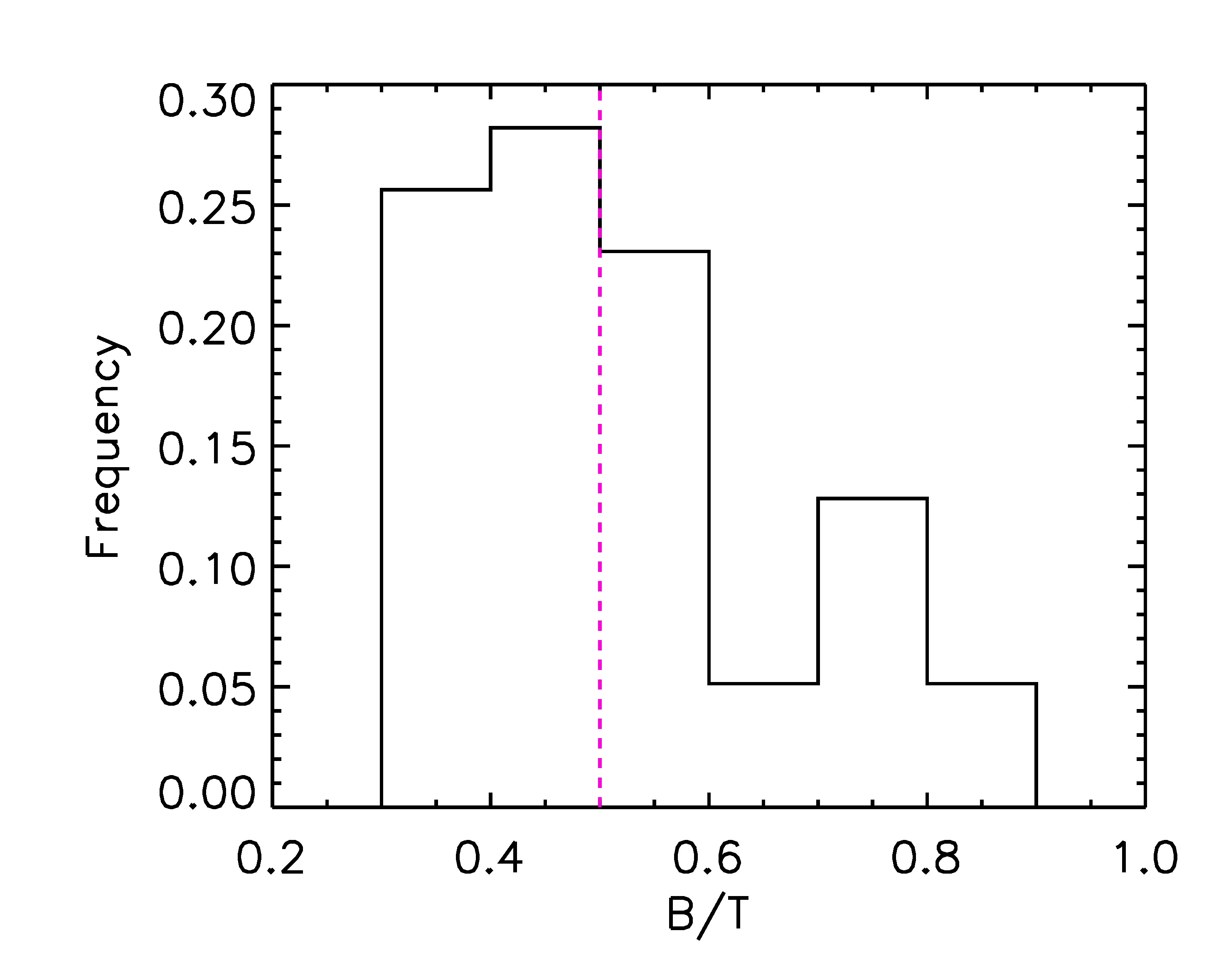
Figure 1: Distribution of the dynamical $B/T$ ratios for the 39 well-resolved simulated galaxies. Only those with $B/T>0.5$ (red dashed line) are classified as SDGs.

After applying the morphological selection, the final sample of SDGs contains 18 objects, with stellar masses in the range $[0.27-6.33]\times 10^{10}\ \ \mathrm{M_{\odot}}$, i.e. all of them are sub-Milky Way mass galaxies. The total stellar mass of the simulated galaxies is obtained by adding the stellar masses of the spheroid and disc components within $R_{\mathrm{opt}}$. We also estimate the stellar half-mass radius, $R_{\mathrm{hm}}$, as the radius that encloses 50% of the total stellar mass. Table 2 summarises the properties of the 18 analysed central spheroid-dominated galaxies. Although our sample is small, we carry out a detailed analysis of the dynamical and astrophysical properties which contribute to understanding the complex history of formation of these galaxies and to set constraints on the subgrid physics. This is of utmost importance, since the interpretation of the observations relies on the comparison with numerical models.

3.2 Spheroid and disc surface mass densities

For the disc and spheroid components, the projected stellar-mass surface density distributions are computed. As we have dynamically separated spheroid and disc components, it is straightforward to fit a Sersic profile (Sersic, 1968) to the projected surface distributions, obtaining the central surface brightness $I_{0}$, the scale radius $R_{\mathrm{b}}$, and the Sersic index $n$:

$$I(R)=I_{0}\exp{\big{(}{-(R/R_{b})^{(1/n)}}\big{)}}$$ (1)

For our analysis the projected stellar-mass surface density is considered a proxy of the luminosity surface brightness (equivalent to adopting a mass-to-light ratio $M/L=1$, which is close to observations for optical-infrared bands). When $n=1$, the Eq. (1) recovers the exponential profile that is fitted to the stellar-mass surface density of the disc components, obtaining in this way the scale length $R_{\mathrm{d}}$ (Table 2).

For the spheroid component, the surface density profiles are fitted within the radial range defined by the gravitational softening and the radius that encloses $90\%$ of the total spheroid mass. In the case of the disc component, the fit is performed within the latter and $R_{\mathrm{opt}}$.

In Appendix A, Fig. 15 shows the synthetic images of the 18 SDGs, the distributions of $\epsilon$, and the projected surface density for the spheroid and disc components, and the corresponding best-fitted profiles. We also include the projected density profiles of those particles supported by rotation but coexisting with the spheroid. As can be seen, these particles determine a variety of surface density profiles: some SDGs have discs which continue exponentially to the central part (e.g. SDG 897), while others get flatter (e.g. SDG 925) or change the profiles to merge with that of the spheroid components (e.g. SDG 790). As mentioned before, with different degrees of importance, all the SDGs have a disc components. In this figure we also include the observability radius. As can be seen in all cases, the disc components are below the observability threshold. This is also seen in the right panels of Fig. 15, where the horizontal dotted lines indicate the stellar surface density of the given galaxy corresponding to the observability radius. Most of the external discs of the simulated galaxies would not be observed in the SDSS galaxy images. In particular, as can be seen from Fig. 15, SDG 288 also has spiral arms. According to the morphological classification of Sandage (1961), this galaxy might not be an ETG. However, according to the dynamical $B/T$ ratio (0.74 in this case), the disc components represents a small fraction of the total stellar mass (i.e. the disc is a tenuous extended rotating system).

As mentioned above, the inner discs that coexist with the spheroids have stellar-mass surface density profiles that behave differently. Some of them follow the exponential profiles of the discs determining a unique exponential profile, while others break off either to follow the spheroid profiles or to set a new flatter trend. We detect that 3 out of the 18 analysed SDGs have discs with stellar-mass surface density profiles following those of the spheroid components. These spheroids have $n\sim 2-3$.

In order to quantify the relative importance of the inner discs with respect to the spheroid components (i.e. defined by the dispersion-dominated stars), we calculate the stellar mass fraction, $F_{\mathrm{rot}}$, of stars with $\epsilon>0.5$ and with binding energies low enough to be classified as part of the spheroid component. This fraction is a measure of the rotating component embedded in the spheroid region. As can be seen from Fig. 2, a clear correlation between $F_{\mathrm{rot}}$ and $B/T$ is found with a Spearman correlation coefficient of $-0.77$ ($p=0.0002$). Figure 2 shows that those systems which overall are more dominated by the spheroid component have a smaller contribution of an inner rotating disc. We note that the dispersion is significant, particularly for those SDGs with $B/T$ $\sim 0.5-0.6$, where $F_{\mathrm{rot}}$ can vary between $\sim 0.2$ to $\sim 0.5$, reflecting very different dynamical assembly histories.

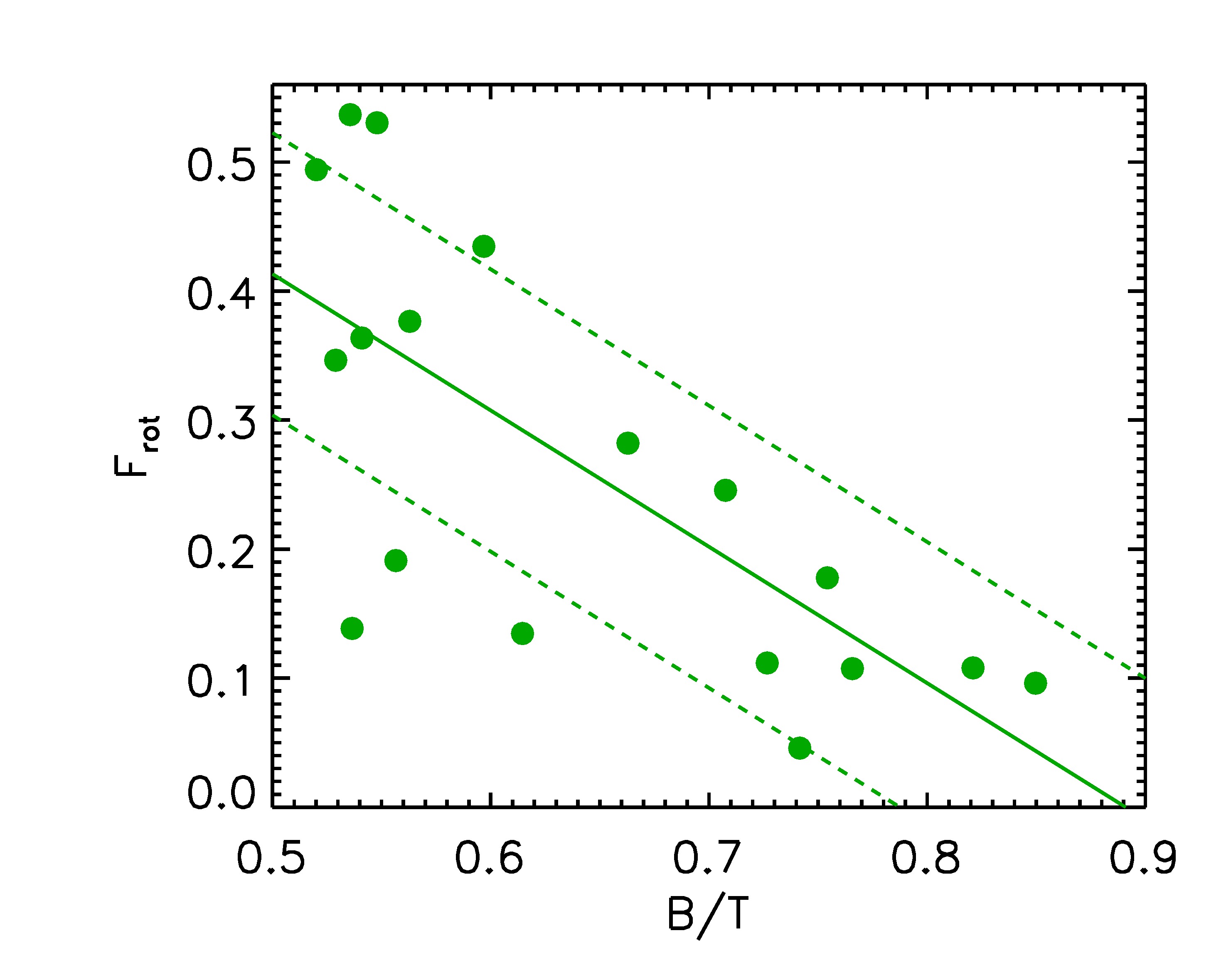
Figure 2: Stellar-mass fractions of the discs that coexist with the spheroidal components as a function of the fraction $B/T$. A linear regression fit is included (green solid line) along with its 1$\sigma$ dispersion (green dashed lines).

The significant variations in the morphologies and the spheroid (bulge)–disc coexistence are the result of the different formation histories. In the following sections, we study these features and to what extent they are able to reproduce observed properties of SDGs.

3.3 Spheroid Sersic index versus $B/T$

As shown in Fig. 3, a correlation is detected between the dynamical $B/T$ ratio and the Sersic index. The Spearman correlation coefficient obtained is $0.63$ ($p=0.01$), implying that the trend is statistically significant, albeit with a large dispersion. A linear regression yields a slope of $5.72\pm 1.89$ and an intercept of $-1.99\pm 1.13$. The errors are calculated by a bootstrap method. The simulated B/T ratios are in a range of values associated with elliptical and lenticular (S0) galaxies. In particular, $\sim 50$% could be classsified as S0 galaxies. Hereafter, we refer to them as spheroidal-dominated systems for the sake of simplicity and because the spheroidal component is always the more massive one. On the other hand, we note that if the stellar mass of the disc coexisting with the spheroid ($F_{\rm rot}$, see Fig. 2) is assigned to the spheroid (as probably done in the photometric bulge/disc decompositions), then the B/T ratios of the simulated galaxies is larger than shown in Figs. 1 and 2.

It has also been claimed that the structural Sersic index, $n$, is able to distinguish between classical bulges and pseudo-bulges, being $n\sim 2$ the value that separates these two types (e.g. Tonini et al., 2016; Fisher & Drory, 2008; Combes, 2009). Not only does this parameter change for the classical and pseudo-bulges, but also many other galaxy properties such as colour, sSFR, rotational support, and kinematics (see Kormendy, 2016, for a recent review). From Fig. 3, we can see that half of our SDGs have $n\leq 2$. These changes and the presence of a disc component inside the spheroids (see above) suggest that the simulated spheroids (bulges) are composite stellar systems formed by the action of different formation channels such as mergers, interactions, or local instabilities (De Lucia et al., 2010; Zavala et al., 2012; Perez et al., 2013, see also Tissera et al. 2017 submitted). The extended discs could grow because our SDGs inhabit low-density environments. In higher density regions, these discs would be prevented from growing or surviving by a higher impact of ram pressure stripping or strangulation.

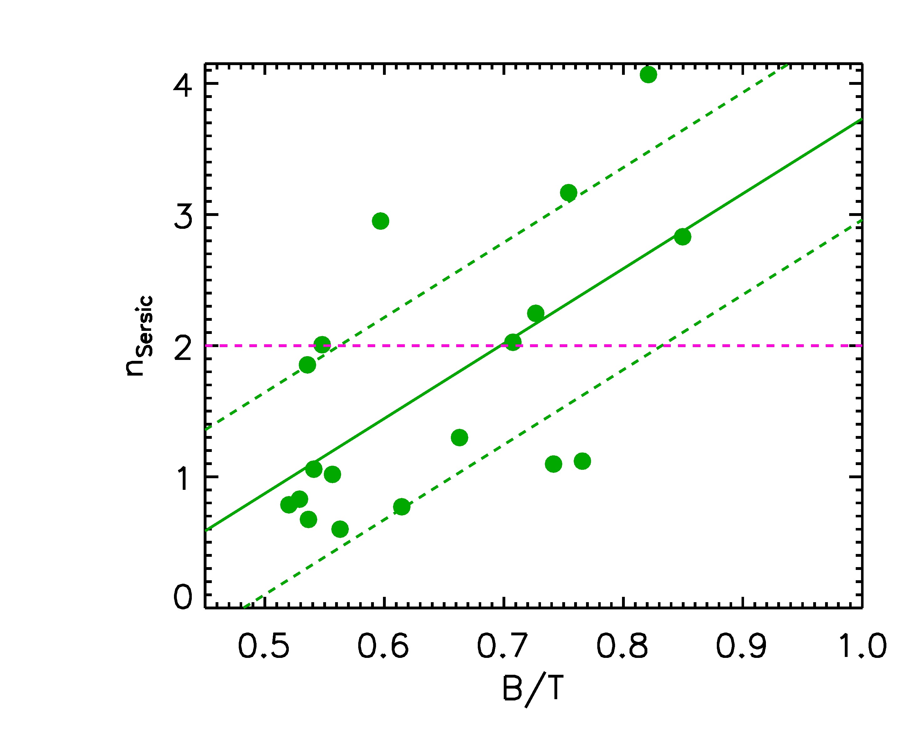
Figure 3: Spheroid Sersic index obtained for the simulated SDGs as a function of their dynamical B/T mass ratios. The green solid and dashed lines represent the best linear regression fit and the 1$\sigma$ dispersion. The magenta dashed line denotes $n=2$, which is often assumed to be the limit between classical and pseudo-bulges.

4 Scaling relations

In this section, we analyse the size-mass relation, the FJR, the FP, and the TFR determined for the simulated SDGs. It is important to analyse these relations since none of them has been used to set the parameters of the subgrid physics modelling, and the degree of agreement (or disagreement) thus provides important clues for improving the models. In all figures in this section, simulated galaxies are distinguished according to the B/T ratio. However, the global relations are calculated over the whole sample in order to have a better statistical estimation.

Since our simulated galaxies are dynamically dominated by the velocity dispersion components, we resort to the samples of observed ETGs from the ATLAS^3D Project (Cappellari et al., 2011, 2013a) and ETGs with $\mathrm{H_{I}}$ disc components identified from the ATLAS^3D survey by den Heijer et al. (2015). The presence of these discs allows rotation velocities to be measured accurately. We compile a clean ATLAS^3D sample by excluding those galaxies that belong to the Virgo cluster since our SDGs are field systems. The clean ATLAS^3D sample is compared with simulated trends when appropiate.

4.1 Size-mass relation

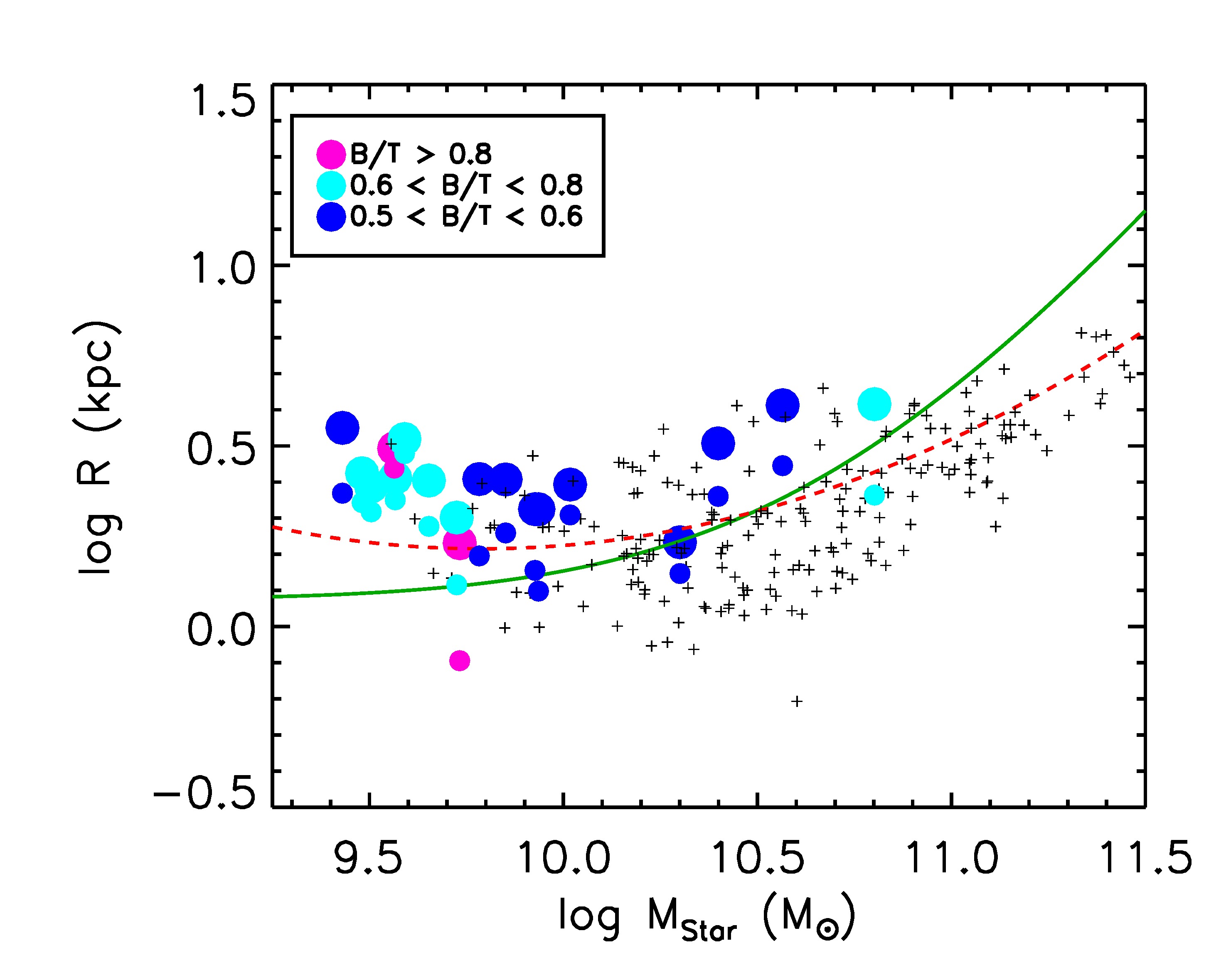
Figure 4: Mass-size relation estimated for the simulated SDGs ($R_{\mathrm{hm}}$, big circles, and $R_{\mathrm{eff}}$, small circles, both coloured according to the dynamical $B/T$ ratios), ETGs from the clean ATLAS^3D sample (black crosses), and the observed relations reported by Mosleh et al. (2013) (green solid line) and Bernardi et al. (2014) (red dashed line) for ETGs.

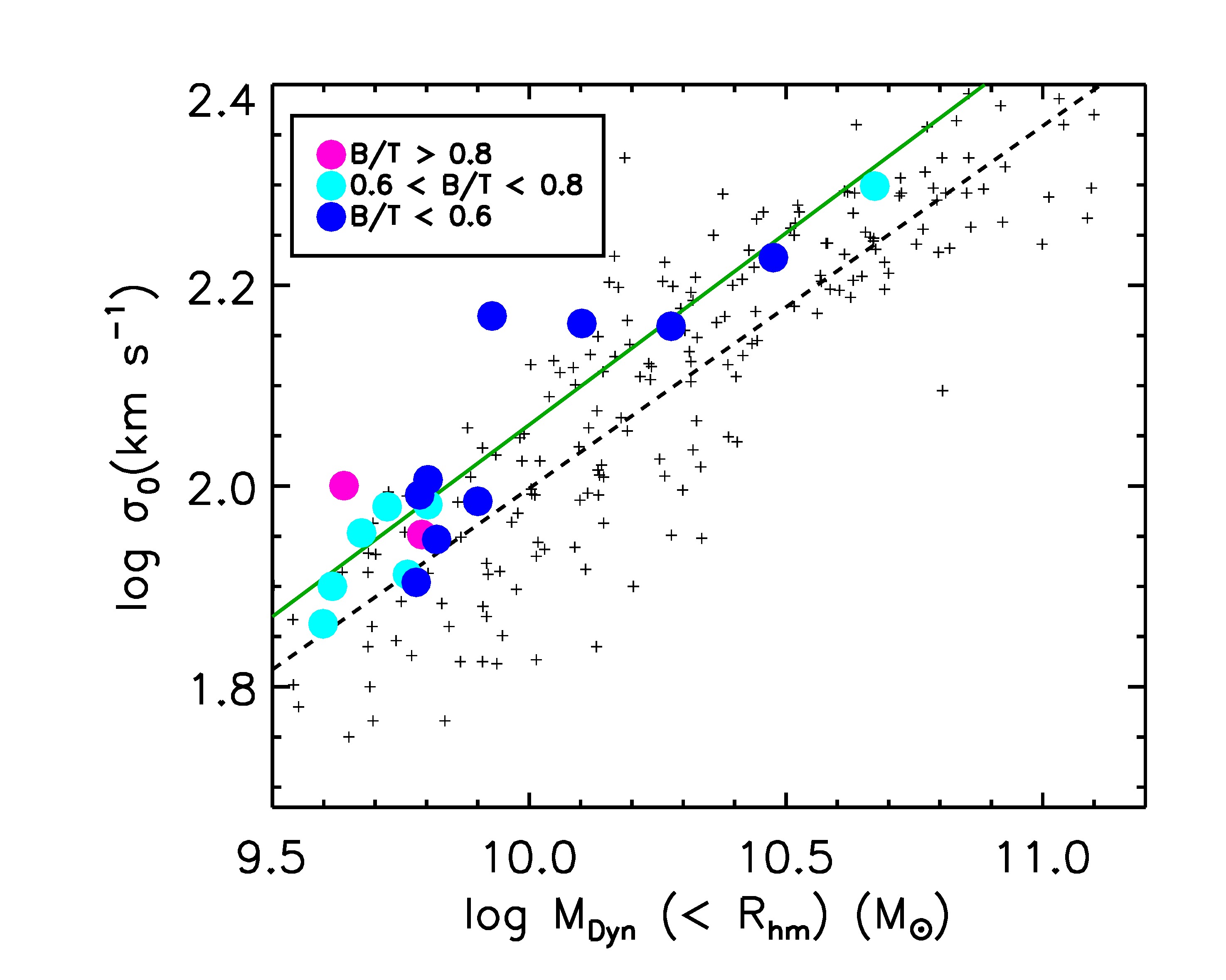
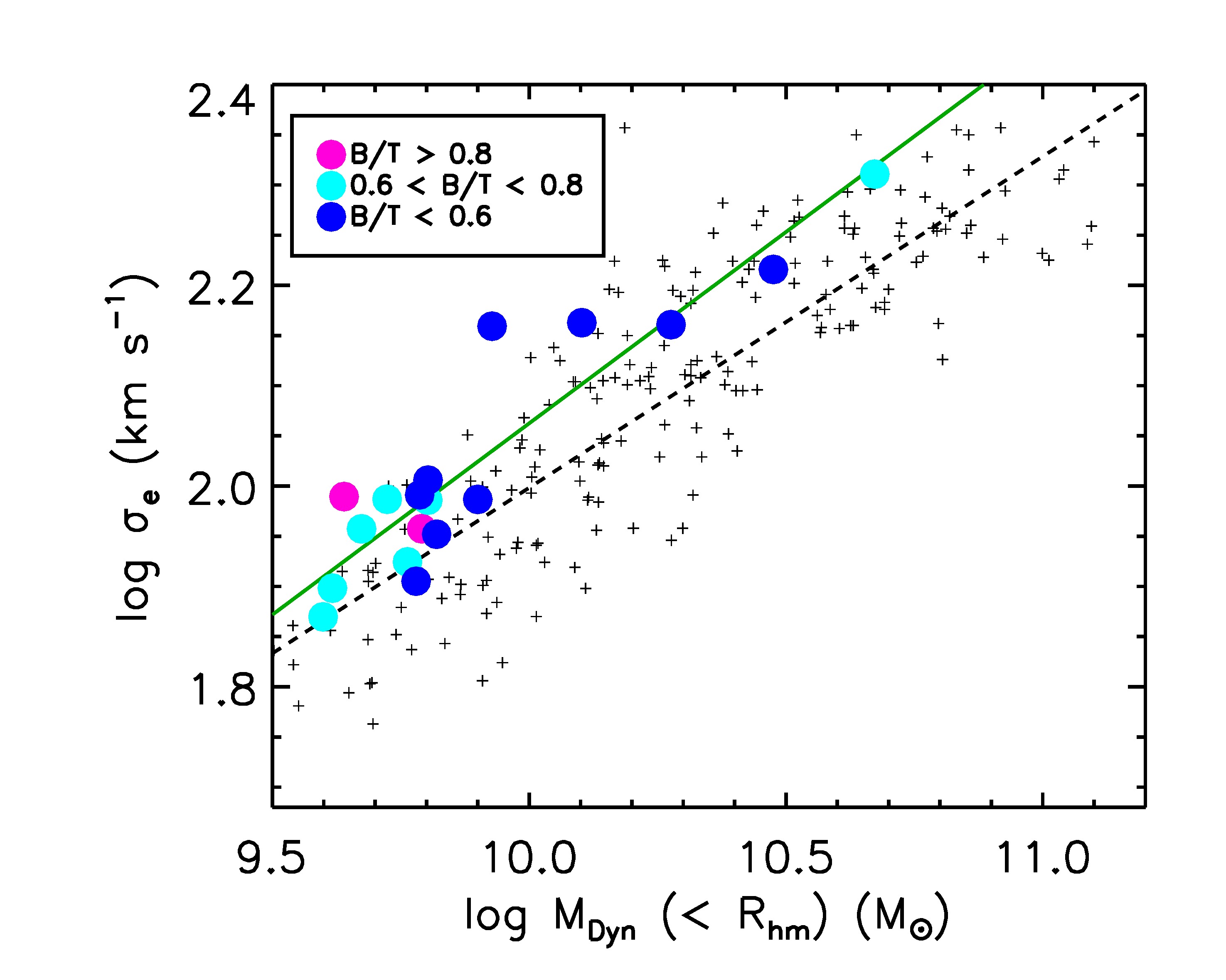
Figure 5: Faber-Jackson relation for the simulated SDGs (filled circles, coloured according to the dynamical $B/T$ ratios) estimated by using $\sigma_{0}$ (left panel) or $\sigma_{e}$ (right panel). For comparison, the corresponding relations obtained from the clean ATLAS^3D sample are included (see Section 4). The linear regression to the simulated data (green solid lines) and observational data (black dashed lines) are depicted for comparison.

One of the fundamental scaling relations is the size-mass relation (e.g. Mosleh et al., 2013; Bernardi et al., 2014). To check that our SDGs satisfy this observed relation, we first use the $R_{\mathrm{hm}}$, which in simulations is straightforward to measure (see above). Observationally, this radius is commonly estimated from an infrared surface brightness profile down to a given aperture (in the infrared the mass-to-light ratio is close to 1) or by fitting a given law to the profile and extrapolating this law to calculate the total galaxy light. Applying a similar procedure, we then define the effective radius $R_{\mathrm{eff}}$. To better compare these data with observations, we use the Sersic profiles fitted to the total surface density obtained by combining the disc and spheroid components within $R_{\mathrm{opt}}$. Then, $R_{\mathrm{eff}}$ is calculated by applying the well-known relation (e.g. Sáiz et al., 2001)

$$\frac{R_{\mathrm{eff}}}{R_{0}}=(2n-0.324)^{n},$$ (2)

which links scale lengths and the Sersic index; $R_{0}$ is the scale length of the Sersic profile fitted as mentioned above.

To compare the simulations with observations, we use the results reported by Mosleh et al. (2013) and Bernardi et al. (2014) for ETGs. Mosleh et al. (2013) have adopted the functional form to relate stellar mass ($M_{\mathrm{Star}}$) and size for spiral galaxies given by Shen et al. (2003)

$$\bar{R}_{\mathrm{eff}}(\mathrm{kpc})\ =\ \gamma\ \bigg{(}\frac{M_{\mathrm{Star}}}{M_{\odot}}\bigg{)}^{\alpha}\ \bigg{(}1+\frac{M_{\mathrm{Star}}}{M_{0}}\bigg{)}^{(\beta-\alpha)},$$ (3)

where $\bar{R}$ is the median of the log-normal distribution of $R_{\mathrm{eff}}$ (in kpc) in stellar mass bins. Mosleh et al. (2013) study a sample selected from the Max-Planck-Institute for Astrophysics (MPA)–Johns Hopkins University (JHU) SDSS (Kauffmann et al., 2003; Salim et al., 2007). The fitted parameters ($\alpha$, $\beta$, $\gamma$, $M_{0}$) vary with morphology, colour, or sSFR. We take those corresponding to ETGs (table 1 in Mosleh et al. (2013)).

Bernardi et al. (2014) also find that the size-mass relation depends on morphology using the SDSS DR7. They calculate $R_{\mathrm{eff}}$ from different fits to the surface brightness profiles finding

$$\mathrm{log}(R_{\mathrm{eff}}{\mathrm{(kpc)}})\ =\ p_{0}\ +\ p_{1}\mathrm{log}(M_{\mathrm{Star}}-0.24)\ +\ p_{2}(\mathrm{log}(M_{\mathrm{Star}}-0.24))^{2}.$$ (4)

From Bernardi et al. (2014) we take the case of a single-Sersic profile fit for ETGs (their table 4). A correction from Chabrier (Chabrier, 2003) IMF to Salpeter (Salpeter, 1955) is applied.

Finally, we also compare the simulated trends with the ETGs from the clean ATLAS^3D sample. The stellar masses are calculated from the luminosities given in table 1 in Cappellari et al. (2013a), using the mass-to-light ratios from table 1 in Cappellari et al. (2013b) for a Salpeter IMF.

In Fig. 4, we show the comparison between the simulated SDGs and the above-described observational estimates. As can be seen the simulated SDGs have $R_{\mathrm{eff}}$ in reasonably good agreement with observations, whereas the $R_{\mathrm{hm}}$ are slightly larger ($\sim 0.2\ \mathrm{dex}$), especially at lower masses. It is possible that these characteristic radii of our simulated SDGs are indeed slightly larger than those of observed ETGs, due to the presence of extended discs in all of the simulated galaxies.

Hence, overall the simulated mass-size relations of the ETGs are in good agreement with observations. We note that Pedrosa & Tissera (2015) reported that the sizes of the DDGs are also in reasonable agreement with observations. These findings suggest that the adopted SN feedback model is able to reproduce the mass-size relations of both types of galaxies without resorting to any fine-tuning.

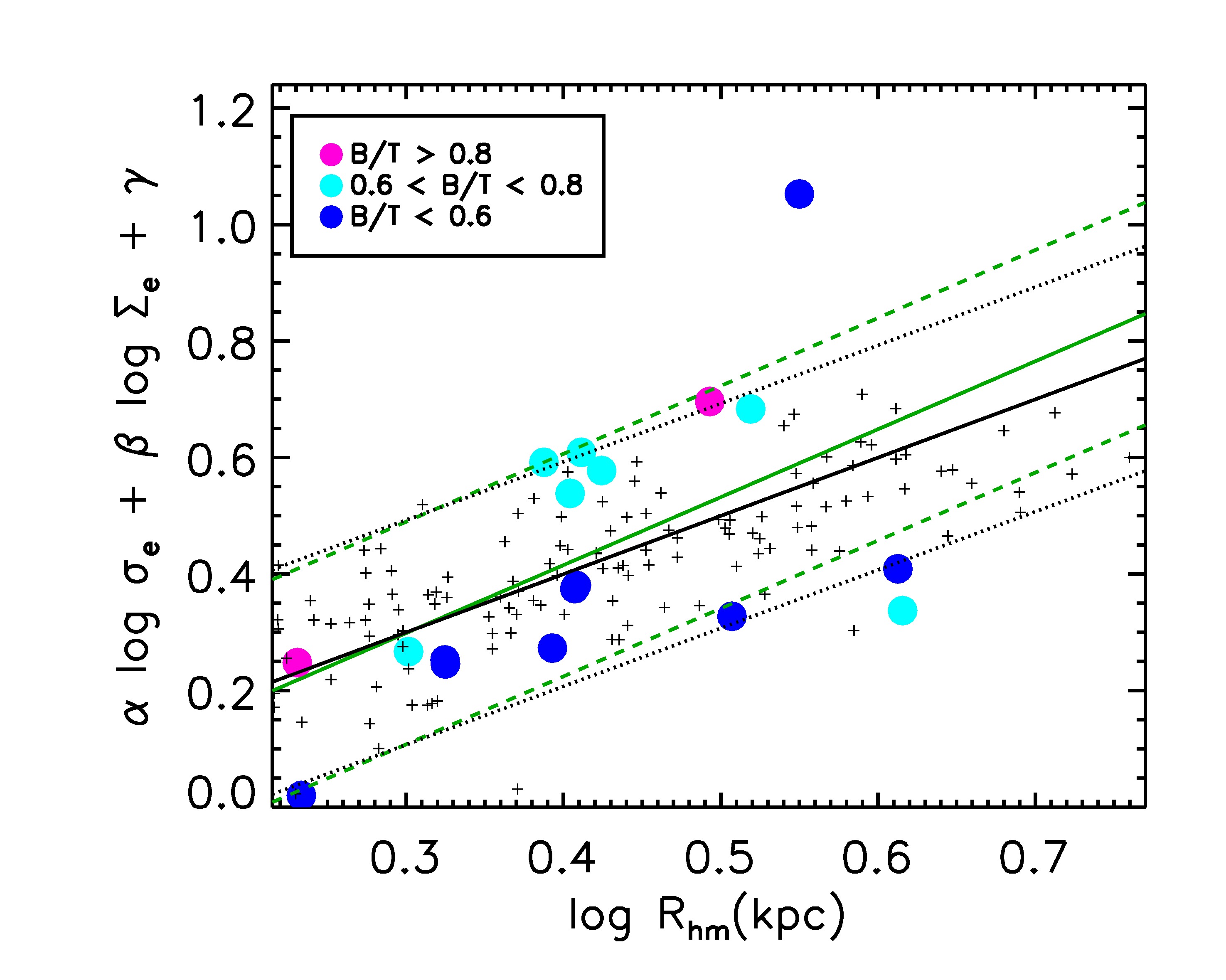
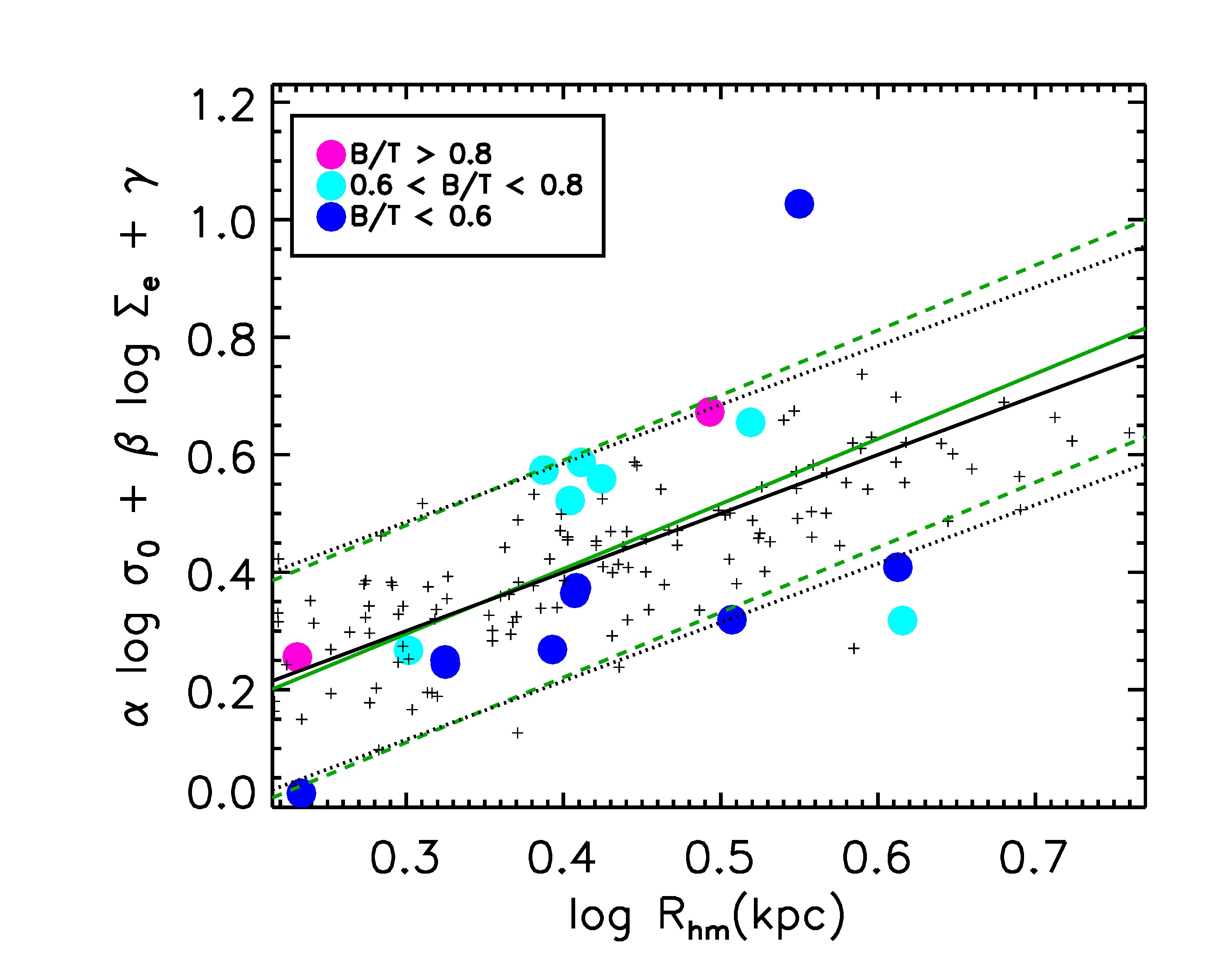
Figure 6: Fundamental plane for the simulated SDGs calculated with the parameters estimated for our clean ATLAS^3D sample. The black line denotes the one-to-one relation and the green line shows the best fit to our simulated SDGs (solid circles, coloured according to the dynamical $B/T$ ratios). The rms is $0.19$ and $0.18$ for the least squares regression (dashed green lines) when considering velocity dispersion within $R_{\mathrm{eff}}$ and central velocity dispersion, respectively, and the corresponding regression for the one-to-one relation (${\it rms}=0.19$ for both cases) is shown by dotted black lines.

4.2 Faber–Jackson relation

The FJR (Faber & Jackson, 1976) relates the luminosity and the central velocity dispersion so that $L\ \propto\ \sigma_{0}^{\gamma}$, where $\gamma$ is a constant. We use the dynamical masses instead of luminosities. For the simulated SDGs, the central velocity dispersion ($\sigma_{0}$) is calculated within $1.5\ h^{-1}$ kpc (corresponding to three gravitational softening radii) and the dynamical masses at $R_{\mathrm{hm}}$. For galaxies in the clean ATLAS^3D sample, the dynamical masses are estimated by following Cappellari et al. (2013a): $M_{\rm JAM}\approx 2\times M_{1/2}$, where $M_{1/2}$ is the total mass within a sphere enclosing half of the galaxy light. To make the conversion to mass, the mass-to-light ratios provided by Cappellari et al. (2013a) are adopted. We also explore whether the same relation holds when the central velocity dispersion is replaced by the velocity dispersion calculated within $R_{\mathrm{eff}}$ ($\sigma_{e}$).

Figure 5 shows both the observational and the simulated FJRs obtained by using $\sigma_{0}$ (left panel) or $\sigma_{e}$ (right panel). The linear regression for the simulated SDGs yields $0.40\pm 0.05$ for both slopes. The errors are calculated via a bootstrap method. Similar linear regression fits to relations defined by the clean ATLAS^3D galaxies yield $0.36\pm 0.01$ and $0.33\pm 0.01$ respectively. Hence, the simulated SDGs follow a FJR in agreement with observations within one standard deviation. No clear dependence is found on the dynamical $B/T$ ratio as can be seen from this figure. We note, however, that our galaxy sample is too small to be able to see a robust trend on this point.

4.3 Fundamental plane

The FP (Dressler et al., 1987; Djorgovski & Davis, 1987; Faber et al., 1987) relates the size ($R_{\mathrm{eff}}$) with the surface density ($\Sigma_{e}$) and velocity dispersion ($\sigma$):

$$R_{\mathrm{eff}}\propto\sigma^{\alpha}\ \Sigma_{e}^{\beta}$$

The surface brightness given by the data available in Table 1 in Cappellari et al. (2013a) is transformed into mass surface densities by adopting $M/L=1$ ($\Sigma_{e}=\frac{L}{2\pi R_{\mathrm{eff}}}$). Similarly to the FJR, the FP is estimated for $\sigma_{e}$ and $\sigma_{0}$.

In Fig. 6 we compare the simulated FP obtained using our clean ATLAS^3D sample. For this sample, using $\sigma_{e}$ for the fit, $\alpha=0.92$ and $\beta=-0.69$ (left panel) for the observed data. When fitting using $\sigma_{0}$, $\alpha=0.87$, and $\beta=-0.66$ (right panel). The black line corresponds to the one-to-one relation ($y=x$). As can be seen, the simulated FP (green lines) is within one standard deviation of the observed relation.

As is well-known, ETGs tend to show a tilt in the FP with respect to the value derived assuming virialisation (Binney & Tremaine, 1987). Its origin is still under debate and there are a variety of possible causes such as a variable or non-homologous IMF (Prugniel & Simien, 1996; Forbes et al., 1998), dependence on dark matter halo features caused by the non-linear assembly of the structure, among others. However, the FP obtained by using dynamical masses is consistent with the predictions from the virial theorem (Cappellari, 2016).

4.4 Tully-Fisher relation

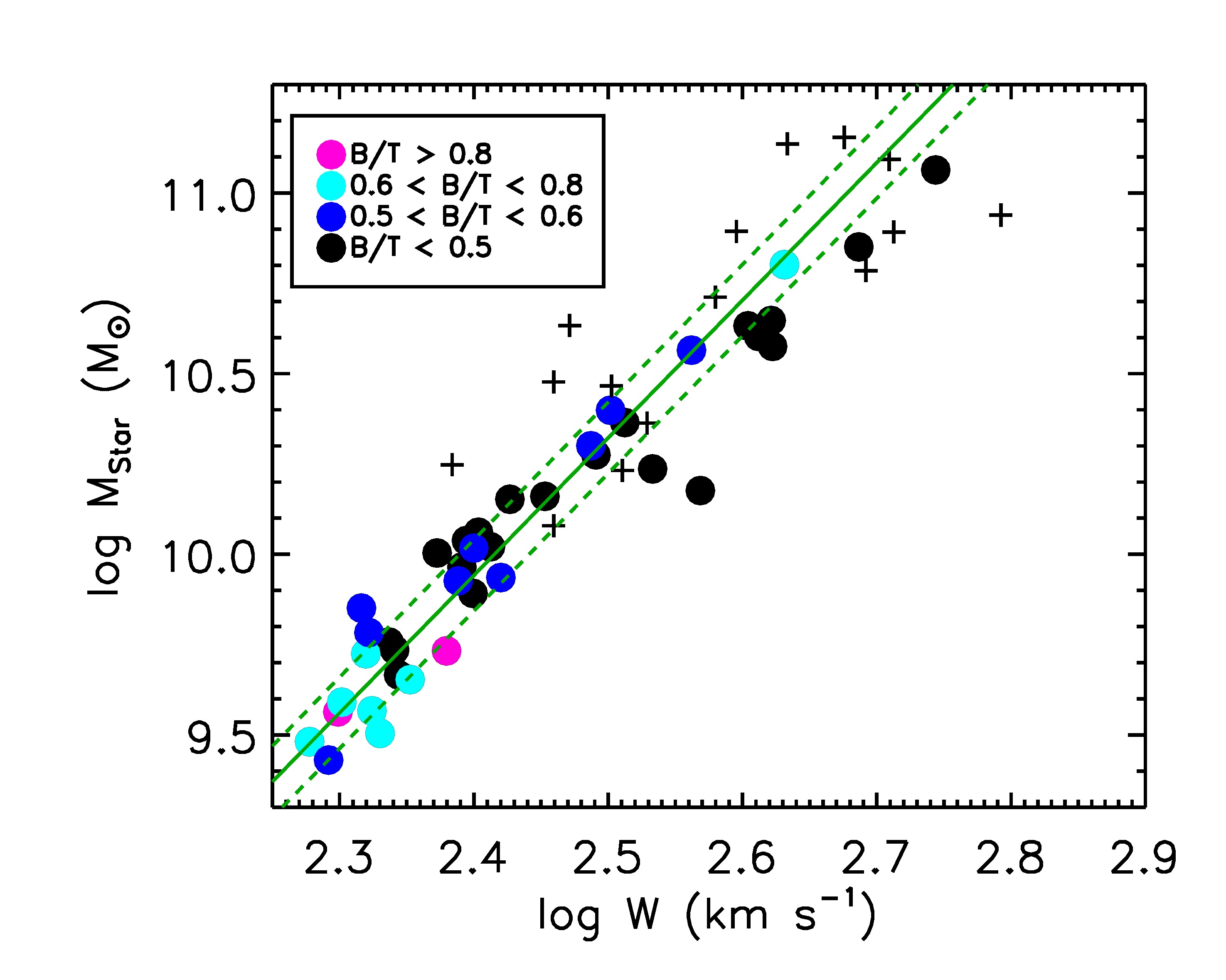
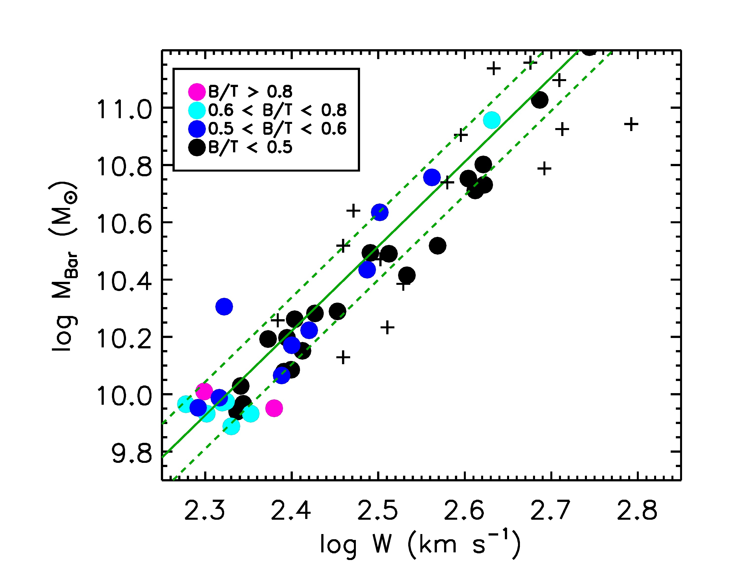
Figure 7: Stellar (left panel) and baryonic (right panel) TFRs for the simulated SDGs (filled circles coloured according to the dynamical $B/T$ ratio) and DDGs (black solid circles), and the observed values reported by den Heijer et al. (2015) for ETGs with extended disc components (black crosses). The linear regression for simulated SDGs (green lines) are shown; the rms dispersions are also shown (dashed lines).

Although ETGs are dominated by a velocity dispersion component, a rotating disc is also frequently detected through cold or ionised gas observations. Emsellem et al. (2011) report most of the ETGs in the ATLAS^3D sample as fast rotators. In particular, den Heijer et al. (2015) study the TFR for 16 ETGs from the ATLAS^3D survey using an extended $\mathrm{H_{I}}$-component which determines a disc component. In this work, the rotation velocity is measured at very large radius (on average, within $R/R_{\mathrm{eff}}=7.3$). We compare this sample with the simulated TFR. For consistency with our previous comparison, a galaxy that belongs to the Virgo cluster has been excluded.

We determine the stellar and baryonic TFRs for our simulated SDGs and fit a relation of the form $\mathrm{log}(M_{i})=a\ (\mathrm{log}(W)-2.6)+b$, where $i$ represents the stellar or the baryonic mass and $W$ is twice the rotational velocity $V$ calculated at twice $R_{\mathrm{opt}}$. The stellar and baryonic masses are determined within $R_{\mathrm{opt}}$. The estimation of stellar masses for the sample of den Heijer et al. (2015, Table 1) is done in the same way as in Section 4.1 by using $r$-band mass-to-light ratios, i.e. their star formation history (SFH) case. The baryonic masses are calculated as the sum of stellar mass and $\mathrm{H_{I}}$ mass multiplied by a factor of $1.4$ to take into account helium and metals (den Heijer et al., 2015).

In Fig. 7 (left panel) we show the stellar TFR. In this case, the linear regression yields $a=3.81\pm 0.20$ and $b=10.70\pm 0.04$ for the simulated SDGs. This is steeper than that reported by den Heijer et al. (2015) ($a=2.40\pm 0.50$ and $10.72\pm 0.06$), but within the scatter and uncertainties involved in the stellar mass determination of the observations and in agreement with the TFR for spiral galaxies. For disc galaxies, it is known that the slope of stellar TFR is steeper than that of the baryonic TFR, and the scatter of the former is smaller than that of the latter (e.g. Avila-Reese et al., 2008). These trends are followed by our simulated SDGs. Our simulated stellar TFR is also in agreement with results from the cosmological EAGLE simulation (Ferrero et al., 2017).

Similarly, Fig. 7 (right panel) shows the baryonic TFR for the simulated SDGs and that reported in den Heijer et al. (2015). The best fitting parameters for the simulated relation are $a=2.95\pm 0.31$ and $b=10.81\pm 0.08$, which are in agreement with the observed values within the estimated errors. In particular, the unconstrained observed TFR (i.e. when they calculate the parameters without fixing any of them), where the baryonic mass is calculated with SFH, yields a slope of $a=2.51\pm 0.42$ and zero-point of $b=10.71\pm 0.05$.

For comparison, in Fig. 7 we include the subsample of simulated DDGs with more than 10,000 baryonic particles (black filled circles). Both the SDG and DDGs follow roughly similar stellar and baryonic TFRs, although disc-dominated galaxies seem to determine a slightly flatter relation in the former case. This might be caused by the action of the SN feedback which is more efficient for lower stellar mass galaxies in the velocity range where most of the SDGs are (De Rossi et al., 2010).

Overall, the main structural and dynamical relations of our simulated SDGs are in reasonably good agreement with those reported for observed ETGs. This is an encouraging result, considering that none of these relations has been fine tuned to be reproduced as mentioned before.

4.5 Dark matter fraction as a function of stellar mass

A key prediction of the $\Lambda$-CDM scenario is that galaxies are embedded in dark matter halos. However, it is not yet clear what the fraction of dark matter within ETGs is. Thanks to integral field spectroscopy studies, like those performed in the ATLAS^3D survey, estimations of $F_{\rm dm}=M_{\rm dm}/M_{\rm dyn}$ are now possible for ETGs (Cappellari et al., 2013b).

In Fig. 8, the $F_{\rm dm}$ measured for our SDGs at $R_{\mathrm{hm}}$ and $R_{\mathrm{eff}}$ are plotted. Since $F_{\rm dm}$ increases with the radius, the values of $F_{\rm dm}$ are higher for $R_{\mathrm{hm}}$ than for $R_{\mathrm{eff}}$ . For both definitions of $F_{\rm dm}$ the smaller the galaxy, the larger the dark matter fraction. This trend is in agreement with the dynamical inference for the ATLAS^3D survey (Cappellari et al., 2013a), as shown in Fig. 8 (for the observed values we have used the stellar masses calculated in Section 4.1). The agreement with the observational inferences is reasonable. However, none of the simulated SDGs has values of $F_{\rm dm}(<R_{\mathrm{eff}})$ smaller than 0.15, while many of the ATLAS^3D ETGs have these values. These are galaxies dominated by baryons and should be very compact in the centre, with high surface densities. The presence of discs in all of our SDGs make them likely less compact.

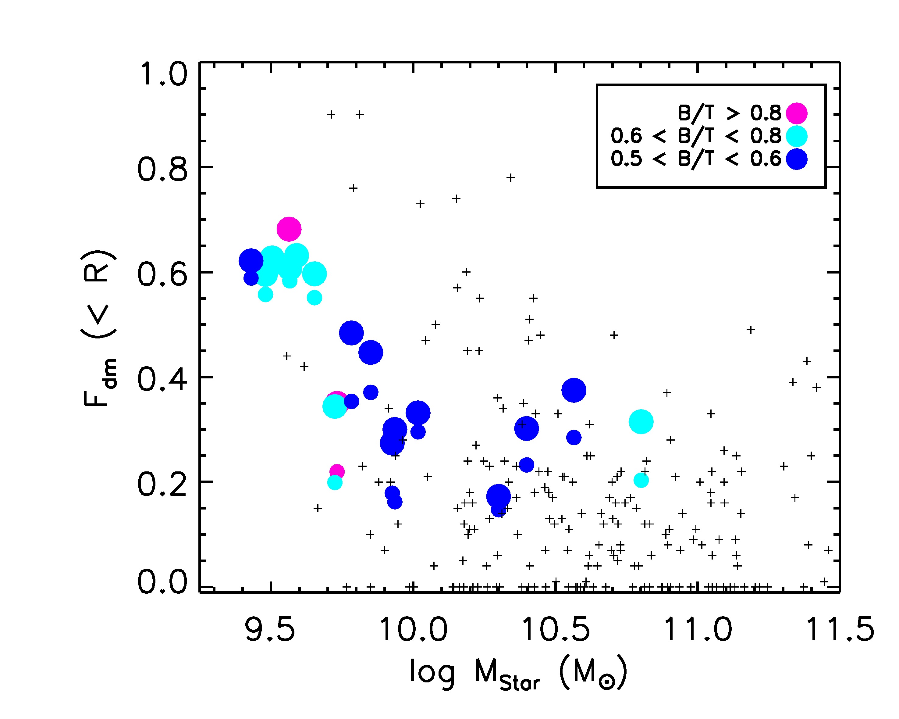
Figure 8: Dark matter fraction, $F_{\rm dm}=M_{\rm dm}/M_{\rm dyn}$, within $R_{\mathrm{hm}}$ (big solid circles) and $R_{\mathrm{eff}}$ (small solid circles), both coloured according to the dynamical $B/T$ ratios as a function of stellar mass for the simulated SDGs. The crosses are dynamical estimates for the ATLAS^3D ETGs (Cappellari et al., 2013a, b).

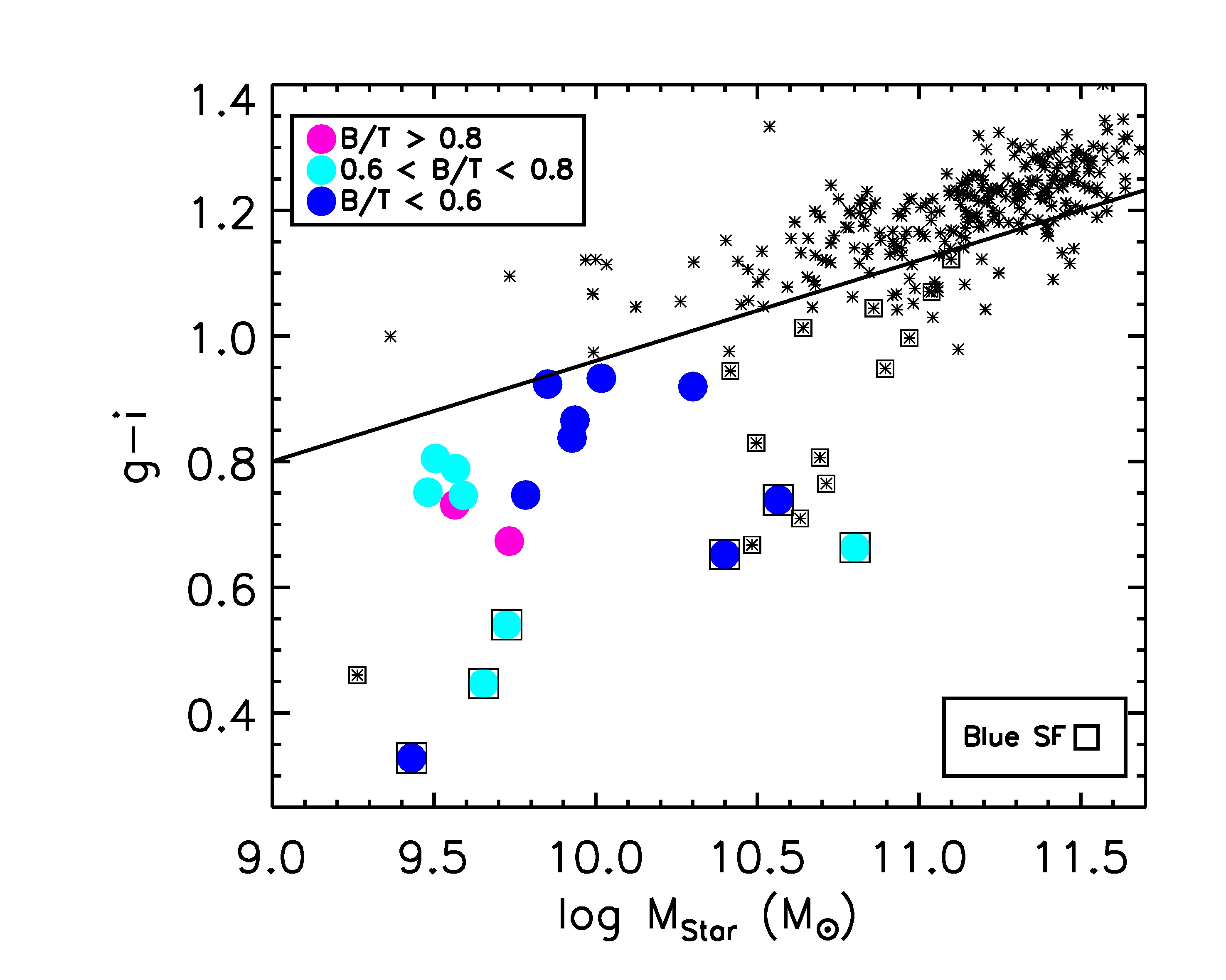
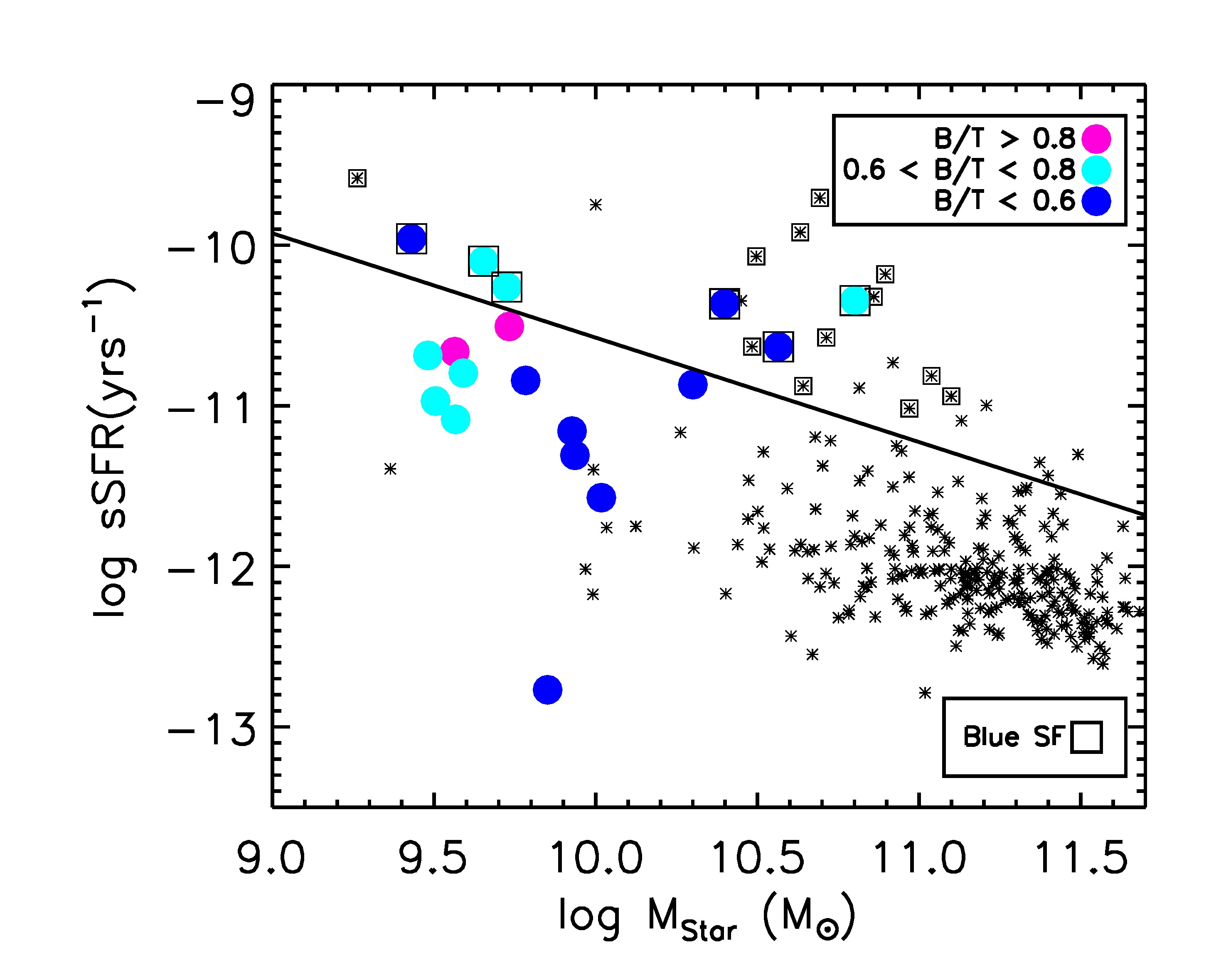
Figure 9: Colours and sSFRs as a function of the $\mathrm{M_{Star}}$ (left and right panels, respectively) for the simulated SDGs (filled circles coloured according to the dynamical $B/T$ ratios). Observational results for isolated ETGs (black asterisks; Hernández-Toledo et al., 2010) are included. In the left panel, blue and red galaxies are separated by the black line reported by Lacerna et al. (2014), while in the right panel the black line depicts the limit between star-forming and passive galaxies (Lacerna et al., 2014). Galaxies that are blue and star-forming at the same time are marked with black open squares.

Table 2: Main properties of simulated SDGs.

ID	$M_{\mathrm{vir}}$	N baryons	$M_{\mathrm{Star}}$	$R_{\mathrm{opt}}$	$R_{\mathrm{hm}}$	$B/T$	$F_{\mathrm{rot}}$	$n_{\mathrm{Sersic}}$	$R_{\mathrm{eff,Sersic}}$	$R_{\mathrm{d}}$	$n$	$R_{\mathrm{eff}}$	sSFR	$g-i$
	$(10^{11}\mathrm{M_{\odot}})$		$(10^{9}\mathrm{M_{\odot}})$	(kpc)	(kpc)				(kpc)	(kpc)		(kpc)	($10^{-11}\mathrm{yr}^{-1}$)
(1)	(2)	(3)	(4)	(5)	(6)	(7)	(8)	(9)	(10)	(11)	(12)	(13)	(14)	(15)
288	20.74	133719	63.34	26.58	4.13	0.74	0.05	1.10	2.26	18.48	1.07	2.31	4.52	0.66
579	10.59	78666	36.73	30.88	4.10	0.54	0.36	1.06	2.20	7.32	1.07	2.79	2.33	0.74
613	7.80	61831	25.05	22.61	3.21	0.53	0.35	0.83	1.63	5.44	0.96	2.29	4.32	0.65
735	4.30	40504	19.97	10.09	1.71	0.56	0.38	0.60	1.06	2.23	0.50	1.40	1.35	0.92
881	2.79	21211	10.41	15.38	2.47	0.52	0.49	0.79	1.47	3.18	0.81	2.04	0.27	0.93
790	3.98	23397	8.62	17.47	2.11	0.60	0.43	2.95	0.96	3.73	3.10	1.25	0.49	0.87
897	2.19	17297	8.45	9.99	2.11	0.54	0.14	0.67	1.19	3.83	1.10	1.43	0.70	0.84
885	2.89	14635	7.10	22.08	2.55	0.55	0.53	2.01	1.41	5.21	1.44	1.82	0.02	0.92
746	2.75	21649	6.07	32.66	2.56	0.54	0.54	1.85	1.03	4.32	2.09	1.57	1.44	0.75
823	3.63	13422	5.40	18.09	1.70	0.85	0.10	2.83	0.79	3.93	2.84	0.80	3.12	0.67
946	2.08	11990	5.31	18.37	2.00	0.66	0.28	1.30	1.12	3.42	1.73	1.30	5.49	0.54
868	2.53	12661	4.50	11.51	2.54	0.61	0.13	0.77	1.49	3.29	1.09	1.89	7.95	0.45
925	2.16	11439	3.89	20.74	3.30	0.71	0.25	2.03	2.54	4.82	1.79	3.01	1.60	0.75
904	2.39	12963	3.69	16.00	2.58	0.73	0.11	2.25	2.43	4.02	1.58	2.24	0.82	0.79
1005	1.78	12609	3.66	20.51	3.11	0.82	0.11	4.07	5.09	5.08	1.71	2.74	2.17	0.73
969	2.25	10405	3.20	14.85	2.44	0.77	0.11	1.12	2.08	3.81	0.86	2.08	1.07	0.81
979	1.71	10713	3.03	23.89	2.66	0.75	0.18	3.17	1.82	5.32	2.59	2.20	2.06	0.75
917	2.76	12325	2.69	19.20	3.55	0.56	0.19	1.02	1.73	4.47	1.13	2.34	10.96	0.33

5 Galaxy colours and specific star formation activity

In this section, we focus on the analysis of the SF activity and the galaxy colours of the simulated SDGs. Integrated magnitudes and colours are computed from the resulting fully integrated spectral energy distribution (SED) of each galaxy, based on its age, mass, and metallicity (for more details see Appendix A). We compare our data with the sample of ETGs (elliptical and lenticular) from the UNAM-KIAS Catalog of Isolated Galaxies (Hernández-Toledo et al., 2010) selected from DR5 SDSS under strict isolation criteria. Lacerna et al. (2016) have studied in detail a subsample of pure elliptical galaxies from the UNAM-KIAS Catalog (see more details therein).

In Fig. 9 (left panel) the $g-i$ colours are plotted against $M_{\mathrm{Star}}$. As can be seen, the simulated SDGs occupy a range of stellar masses shifted to lower masses with respect to the bulk of the observations, but in the mass interval where they overlap the simulated galaxies are clearly bluer than the observed ones. The black line separates blue and red galaxies according to a relation presented in Lacerna et al. (2014),

$$g-i=0.16\ [\mathrm{log}(M_{\mathrm{Star}})-10.56]+1.05,$$ (5)

where $M_{\mathrm{Star}}$ is in units of M_⊙, and the masses were corrected to a Salpeter IMF (Salpeter, 1955). All the simulated SDGs lie on the blue side of the $g-i$ versus $M_{\mathrm{Star}}$ relation, while most of the observed isolated pure ETGs are in the red sequence. In particular, only $20\%$ of these observed galaxies in the same mass range (approximately $[10^{9.4},10^{10.8}]\ \mathrm{M_{\odot}}$) are blue. The blue colours of simulated SDGs are consistent with a more important contribution of young stellar populations.

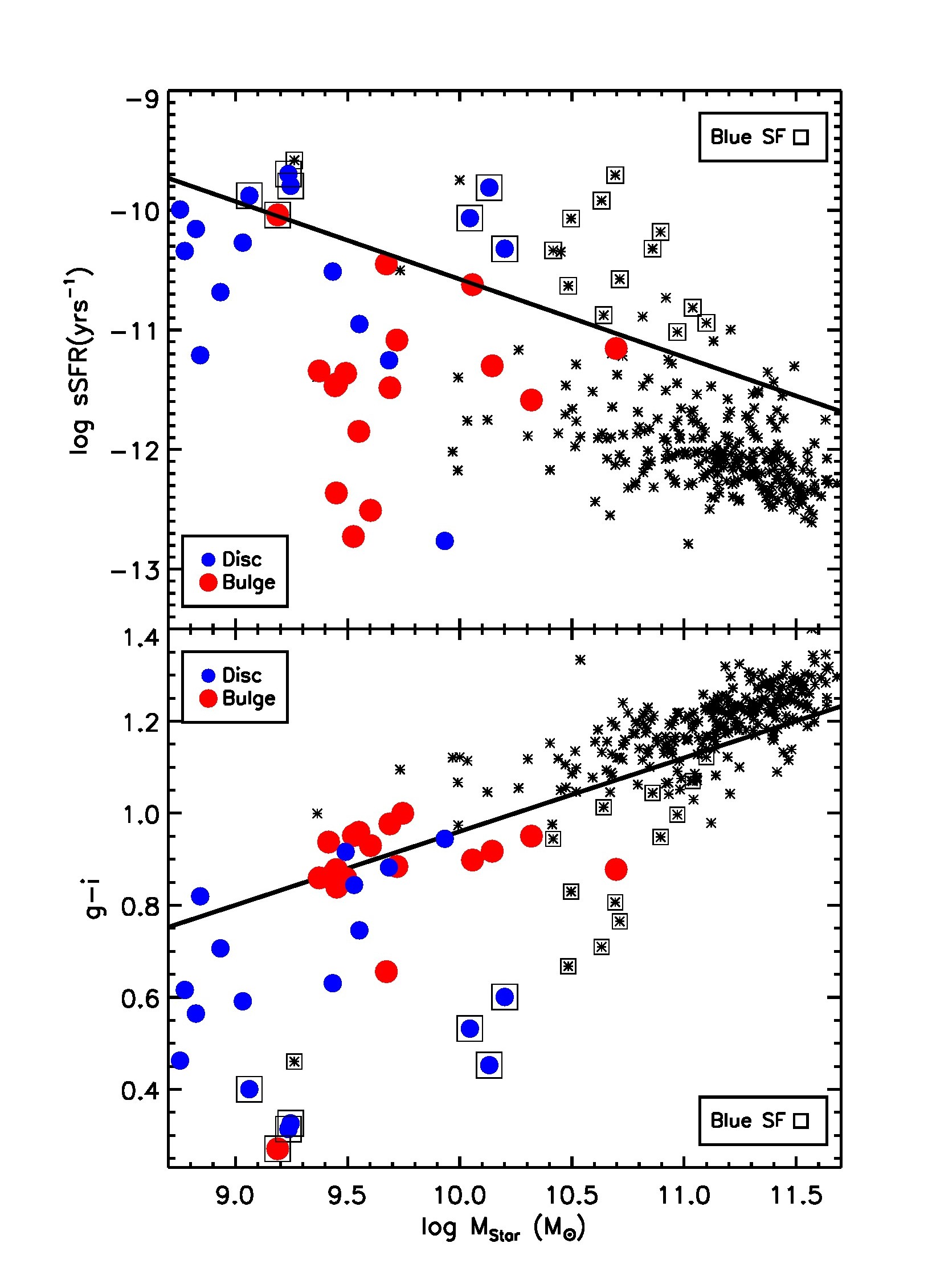
Figure 10: Properties of the spheroid (red circles) and disc (blue circles) components: $g$–$i$ (top panel) and sSFR (bottom panel) as a function of $\mathrm{M_{Star}}$. For comparison, we include the same observations as in Fig. 9 (black asterisks). We depict blue star-forming galactic objects as black open squares, and the limiting lines reported by Lacerna et al. (2014) between red and blue galaxies in the top panel, and between star-forming and non-star-forming galaxies in the bottom panel.

To investigate the SF activity of the simulated galaxies and the relation with the colour distributions, we calculated the SFR by using stars younger than 1 Gyr. This SFR is not an ‘instantaneous’ measure of the activity, but we choose it because it is less affected by numerical noise than measures using lower ages given that most of the SDGs have low values of SFR at $z=0$.

In Fig. 9 (right panel), we plot sSFR (=SFR/$M_{\mathrm{Star}}$), as a function of $M_{\mathrm{Star}}$. The black line separates passive and star-forming galaxies according to Lacerna et al. (2014),

$$\mathrm{log}(\mathrm{sSFR})=-0.65\ [\mathrm{log}(M_{\mathrm{Star}})-10.56]-10.94,$$ (6)

where $M_{\mathrm{Star}}$ is in units of $\mathrm{M_{\odot}}$ and sSFR in units of yr^-1 (corrected for Salpeter IMF). There are 6 out of 18 SDGs ($\sim 33$ %) in the star-forming region, while the rest are below the demarcation line and follow the same trend. With respect to the isolated ETGs from the observations (Hernández-Toledo et al., 2010), our simulated SDGs are about $\sim 0.5-1$ dex more active. The six star-forming SDGs are highlighted with a blue open square in this figure and in the following ones. As can be seen in both panels of Fig. 9, the fraction of simulated blue star-forming SDGs is higher than the observed fraction for isolated ETGs ($33$ % vs. $14$ % in the same mass range).

5.1 Properties of spheroids and discs

Because each simulated SDG has been decomposed dynamically into a spheroid and a disc component, similar estimations of colours and sSFRs as presented above can be performed for each of these components. In particular, we explore whether the colours and sSFR of the spheroids would agree more closely with observations.

In Fig. 10 we show the sSFR and $g$–$i$ colour as a function of the stellar mass for the disc and spheroid components. The differences between the two components are evident. The disc components of the simulated SDGs are nearly all blue according to Lacerna et al. (2014) and with high sSFR (there are only two red discs and both of them are passive), whereas the spheroid components show redder colours and much lower sSFR values, as we expected. We find $\sim 39$ % of the spheroids are red and $\sim 94$ %  are quiescent. In the mass range in common with the observations, $[10^{9.4},10^{10.8}]\ \mathrm{M_{\odot}}$, $\sim 50$ %  of the spheroids are red and all are quiescent (except only one which is just above the limit). Therefore, comparing these fractions with those of observed isolated ETGs in the mentioned mass range, we find that the star formation activity of the spheroids are in rough agreement. However the colours of the simulated spheroids are still bluer than observations ($\sim 80$ %).

Table 3: Fraction of young stars in the spheroid and disc components.

ID	Spheroid			Disc
	¡ 2 Gyr	¡ 3 Gyr	¡ 4Gyr	¡ 2 Gyr	¡ 3 Gyr	¡ 4Gyr
288	0.01	0.03	0.04	0.31	0.50	0.64
579	0.01	0.01	0.01	0.09	0.14	0.16
613	0.01	0.02	0.12	0.19	0.38	0.54
735	0.03	0.05	0.08	$\sim$ 0	$\sim$ 0	0.02
881	$\sim$ 0	$\sim$ 0	$\sim$ 0	0.02	0.03	0.08
790	0.02	0.02	0.06	0.04	0.19	0.35
897	0.01	0.01	0.01	0.02	0.04	0.08
885	$\sim$ 0	$\sim$ 0	$\sim$ 0	0	0	0.01
746	$\sim$ 0	$\sim$ 0	$\sim$ 0	0.07	0.14	0.21
823	0.09	0.16	0.22	0.02	0.04	0.09
946	$\sim$ 0	$\sim$ 0	0.01	0.19	0.20	0.26
868	0.01	0.01	0.07	0.39	0.61	0.69
925	$\sim$ 0	0.02	0.05	0.14	0.32	0.43
904	0.02	0.03	0.05	0.10	0.20	0.23
1005	0.02	0.02	0.03	0.22	0.24	0.24
969	$\sim$ 0	$\sim$ 0	$\sim$ 0	0.09	0.14	0.17
979	0.01	0.02	0.03	0.14	0.18	0.20
917	0.16	0.21	0.28	0.42	0.47	0.51

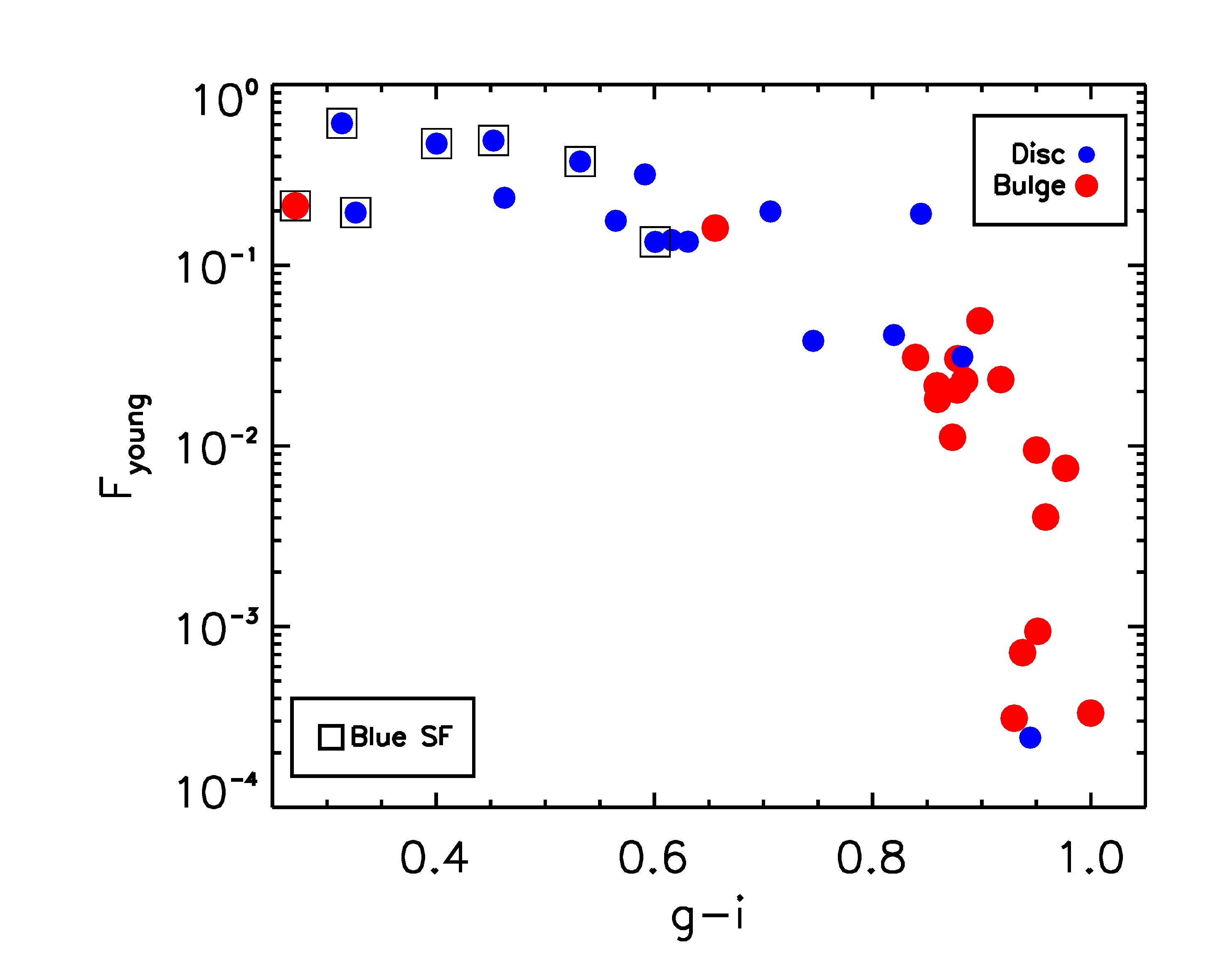
Figure 11: Fraction of stars younger than 3 Gyr as a function of the $g$–$i$ for the spheroid (large red circles) and disc (small blue circles) components. We also depict blue star-forming galaxies with open black squares.

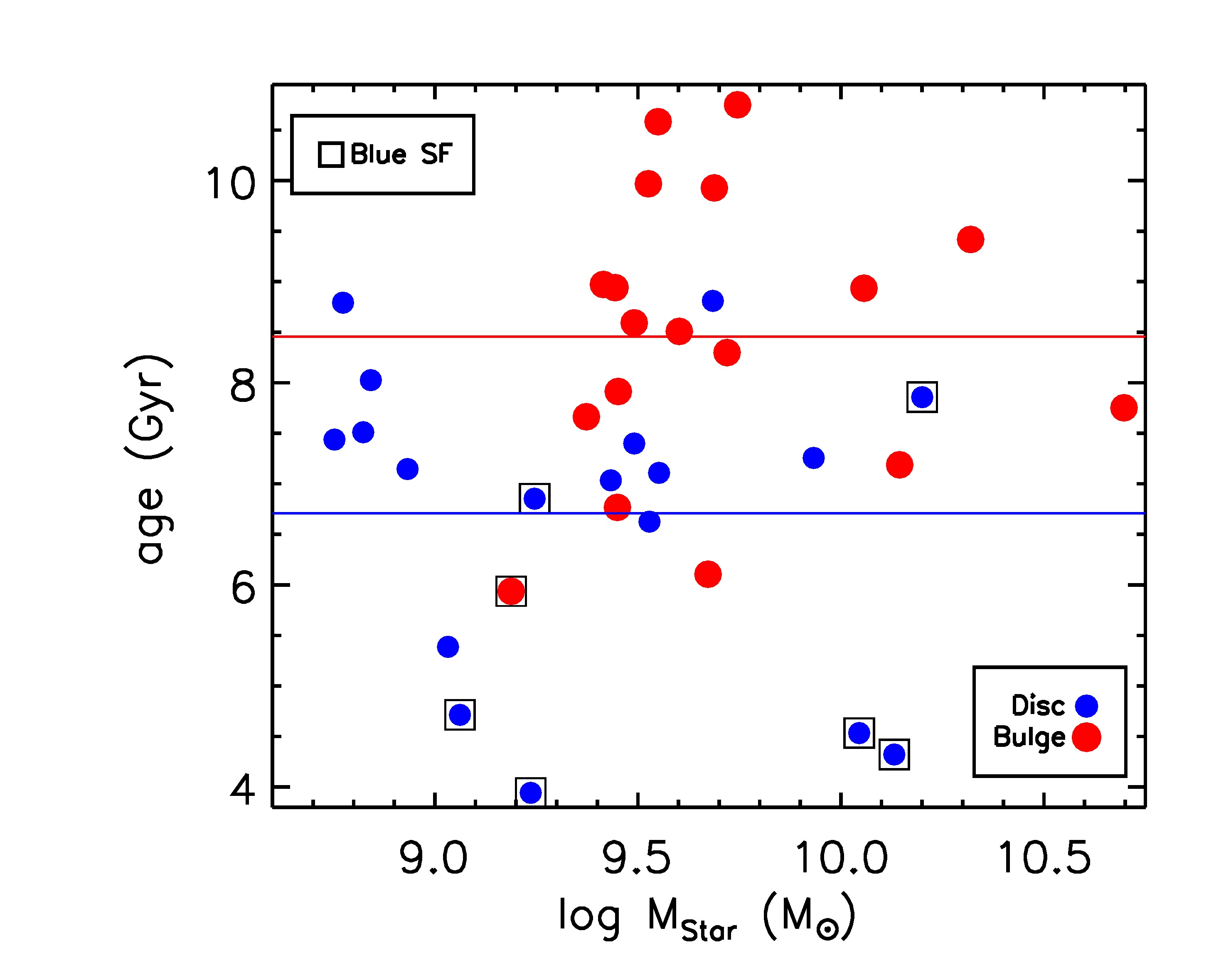
Figure 12: Average mass-weighted ages of the stellar populations in the spheroid (large red circles) and disc (small blue circles) components of the SDGs. The horizontal lines represent the average ages of all spheroids (red) and discs (blue).

As expected, the disc components form stars more actively than the spheroids. This can be quantified by estimating the fraction of young stars. In Fig.11 we show the distribution of the fraction of stars younger than 3 Gyr as a function of $g-i$ for the spheroid and disc components. It is clear that most spheroids have no recent SF, while the discs show the opposite, i.e. that most of them have experienced more recent active episodes, except a single disc which does not have stars younger than 3 Gyr (not shown in Fig. 11). A similar trend is found when a 2 Gyr threshold is adopted instead. In Table 3 the fractions of young stars using different age thresholds are given. The colours of the spheroids are not as red as expected and this is due to the presence of an intermediate-age stellar populations of about 3-4 Gyr old that, although small, it is enough to make colours bluish.

We can also estimate the average ages of the stars in the spheroid and disc components of the simulated SDGs. Figure 12 shows these distributions. As expected, the disc components are younger (horizontal lines correspond to each group average age) than the spheroids: $\sim 6.7$ Gyr compared to $\sim 8.5$ Gyr. There is not clear dependence of the mean ages on the stellar mass in agreement with the results reported by Lacerna et al. (2016).

Our findings show that the simulation produces field SDGs which are globally bluer and more star-forming than observed isolated ETGs, mainly due to the persistence of a disc component in all of them. We note, however, that even for the spheroid components the simulations show a trend where an excess of blue systems is formed, with a significant fraction of intermediate-age stellar populations. Some extra mechanisms for avoiding further disc growth and/or efficiently quenching SF seem to be necessary. For our most massive simulated galaxies, the inclusion of AGN feedback could work in this direction. Simulations of massive galaxies with AGN feedback have shown that the SF rate is reduced whilst this feedback is active (e.g. Khalatyan et al., 2008; Grand et al., 2017). As a result, the galaxies end with a lower fraction of intermediate-age stars that are redder than when AGN feedback is not included. Dubois et al. (2013) have shown that in the absence of AGN feedback, a large number of stars accumulate in the central galaxies to form overly massive, blue, compact, and rotation-dominated galaxies; instead, when AGN feedback is included, these blue massive LTGs turn into red ETGs. However, Newton & Kay (2013) and Park et al. (2017) have explicitly shown that the reduction in SF is significant only for merging galaxies (which is common for massive halos), mainly because the AGN feedback heats the gas and prevents the formation of a new disc, eliminating the possibility of a SF burst that would otherwise happen. For Milky Way-sized galaxies without mergers or with minor mergers, the effect of AGN feedback is minor for the SF history. All analysed galaxies are sub-Milky Way systems, so the effects of AGN feedback is expected to be minor.

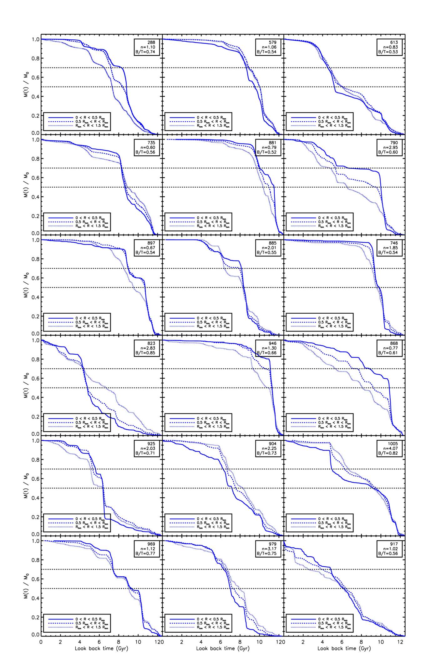
Figure 13: Normalised MGHs estimated in three radial intervals of our 18 SDGs, in order of descending stellar masses (from left to right and from top to bottom). In each panel, the $n_{\mathrm{Sersic}}$ parameter and the dynamical $B/T$ ratio are also included.

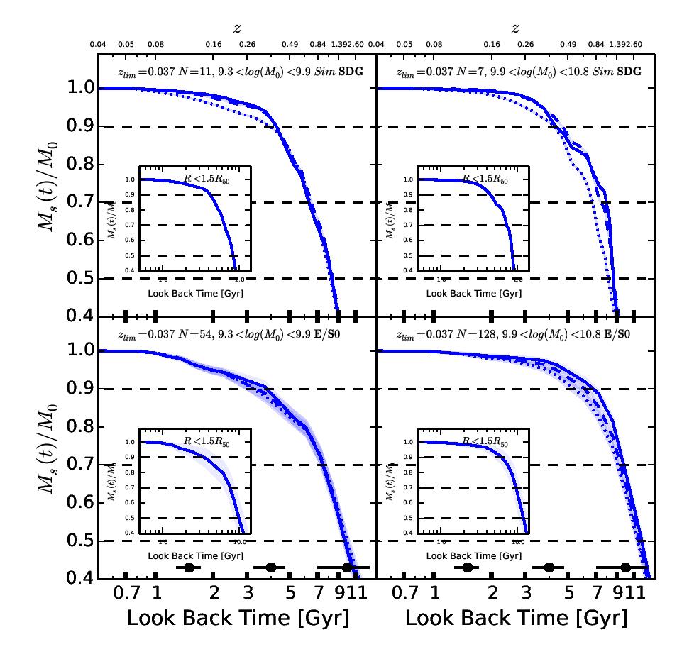
Figure 14: Average global and radial normalised MGH for our simulations (top) and MaNGA ETGs at $z<0.037$ (bottom). We make the division between low (left panels) and high (right panels) stellar mass, adopting $\mathrm{log}(M_{\mathrm{Star}})=9.9$ as a threshold. Radial bins of [0–0.5], [0.5–1.0], and [1.0–1.5] $R_{\mathrm{hm}}$ are represented by solid, dashed, and dotted lines, respectively.

6 Stellar mass growth histories

In this section, we analyse the global and radial ‘archaeological’ mass growth histories (MGHs) of the simulated SDGs. This study provides clues to the galaxy assembly in a cosmological framework and allows a direct comparison with observational findings obtained from integral field spectroscopy. Ibarra-Medel et al. (2016) have analysed galaxies over a wide mass range from the first data release of the Mapping Near Galaxies at APO (MaNGA; Bundy et al., 2015; SDSS Collaboration et al., 2016) survey from SDSS-IV (Blanton et al., 2017). These authors confirm that the global MGHs significantly depend on stellar mass: the more massive the system, the earlier their stars formed on average (downsizing). They have also found that the way galaxies radially grow their stellar masses depends significantly on galaxy morphology, sSFR, or colour. Regarding ETGs, Ibarra-Medel et al. (2016) have found that for a given mass they assemble earlier than late-type galaxies, but also follow a clear downsizing trend. The radial MGHs of ETGs are more homogeneous than those of late-type galaxies (LTGs). On average, the radial MGHs tend to follow a weak inside-out behaviour, but individually there are many cases where the outer regions can be younger than the innermost ones, suggesting either an outside-in assembly at some epochs or processes of global stellar migration from inside to outside. Paths involving inside-out or outside-in scenarios have been reported (e.g. Sánchez-Blázquez et al., 2007). Currently, the formation of spheroidal systems is expected to be a complex process as different mechanisms can contribute, such as gas collapse and infall, mergers, and internal dynamical processes (for recent reviews, see e.g. Brooks & Christensen, 2016; Kormendy, 2016).

Ibarra-Medel et al. (2016) analysed 454 galaxies at $z<0.037$. The global MGHs and those in radial bins were normalised to their corresponding final masses at $z=0.037$ (look-back time of $\sim 0.5$ Gyr); fixing the same final epoch for all galaxies is necessary for calculating the mean MGHs. They explore the dominant direction of mass growth as a function of mass or morphology.

We perform a similar archaeological analysis of our SDGs to that of Ibarra-Medel et al. (2016). The age distribution of the stellar particles at $z=0$ is used to construct the MGHs. In Fig. 13 the normalised MGHs in three radial bins for the analysed galaxies are plotted. The radial bins are defined at [0–0.5], [0.5–1.0], and [1.0–1.5] $R_{\rm hm}$. The panels are in order of decreasing total stellar masses (from left to right and from top to bottom).

As can be seen in Fig. 13, most of systems experience periods of fast growth in the cumulative mass distributions associated with mergers and starbursts. The rates of growth are quite different among the SDGs, with weak dependence on mass. In general, our SDGs show an inside-out formation mode although there is a large variety of behaviours when looked at in detail. Some systems exhibit a combination of modes in their radial MGHs (e.g. SDG 735, SDG 885, SDG 925), while a few galaxies show a clear outside-in mode (e.g. SDG 904).

In Fig. 14 we plot the average global and radial MGHs of the simulated SDGs (upper panels) and the MaNGA ETGs (E/S0; lower panels) in two mass ranges. In this case, the MGHs are normalised and start at a look-back time of 0.5 Gyr (see above). The average radial MGHs of the more massive SDGs attain 70% of their masses at look-back times $\approx 8,7,$ and 6 Gyr for the inner, intermediate, middle and outer radial bins, respectively, while for the less massive SDGs this happens at 6.2, 6.4, and 6.1 Gyr, respectively. The radial MGHs show an average trend of inside-out growth mode, though very moderate. For the massive SDGs, the outer MGHs (dotted line) are shifted to later times with respect to the inner MGHs. For the less massive SDGs, this happens only at late times.

The global average MGHs (insets in Fig. 14) of the simulated SDGs are shifted to later times with respect to those inferred from observations, in particular at the earliest epochs. As discussed in Ibarra-Medel et al. (2016), the fossil record determinations for the oldest ages are very uncertain (see horizontal error bars in the lower panels) and likely bias the stellar population ages to even older values. Both observations and simulations show evidence of mass downsizing, but for the latter the trend is weaker. Regarding the radial MGHs, the simulated galaxies show evidence of a more pronounced inside-out growth mode than observations.

In summary, the simulated SDGs tend to form their stellar populations slightly later and with an inside-out radial growth mode slightly more pronounced than the inferences obtained from the fossil record method applied to MaNGA ETGs. This is in line with the fact that our SDGs are on average bluer and more star-forming than observed isolated ETGs (see previous section). We also note that all the simulated SDGs present a disc component. The SDGs with $\log(M_{\mathrm{Star}})\lesssim 10$ are gas-rich galaxies with a mean gas fraction of 34 % within the optical radius. More massive galaxies show gas fractions around 18 %. These gas fractions are more typical of LTGs (e.g. Calette et al. submitted). The larger gas fractions can account for a more active SF activity. In a previous work, De Rossi et al. (2013) find that the SN feedback adopted in this simulation is able to regulate the SF activity in galaxies with rotational velocity smaller than $\sim 100\ \mathrm{km\ s^{-1}}$ so that these systems reach an equilibrium point where the SN feedback produced by a mild SFR is enough to keep the gas turbulent and warm and at the same time allows the SF to be fed smoothly. Observational constraints on the gas fraction and the SF history of ETGs galaxies in this stellar mass range would be important to further improve the SN feedback models.

7 Conclusions

We have analysed the properties of simulated galaxies dominated by the spheroid components in a $\Lambda$-CDM universe with the aim to investigate to what extent these systems are consistent with the observations. In previous works, the dynamical and chemical properties of disc-dominated galaxies have been studied in great detail, finding very good agreement with observations (Pedrosa & Tissera, 2015; Tissera et al., 2016a, b, 2017). Since the evolutionary paths of spheroid-dominated galaxies are expected to be different, it is of relevance to assess to what extent the same models and simulations reproduce the two kinds of systems.

After identifying the velocity dispersion-dominated spheroid and the rotation-dominated disc by means of a dynamical criterion, we classify our simulated (field) galaxies as SDGs as those with $B/T>0.5$. We notice that all our SDGs actually have an extended disc component, although all of them are found to be below the SDSS observability limit, and that an inner disc component coexists with a spheroid. It is important to keep in mind these particularities when explaining the differences between observed galaxies and our simulations. The main results from our analysis are as follows:

1. The values of the spheroid Sersic index increases on average with the dynamical $B/T$, in agreement with observational results (e.g. Fisher & Drory, 2008).

2. The sizes of the simulated SDGs as a function of $M_{\rm Star}$ are consistent with observational determinations. We measure both $R_{\rm hm}$ directly from the simulation and $R_{\rm eff}$ from the Sersic fits to the whole galaxy. While the former radii are slightly larger ($\sim 0.2$ dex) than the observational estimates, specially at low masses, the latter agree with them.

3. The dynamical relations of our SDGs are in reasonable agreement with observational results for ETGs. The FJR defined as the correlation between $\sigma$ (central or at $R_{\rm hm}$) and the dynamical mass at $R_{\rm hm}$ has a slope of $\sim 0.4$, in good agreement with the ATLAS^3D ETGs (Cappellari et al., 2013a). SDGs also exhibit a tilt in the FP consistent with these observations. The stellar and baryonic TFRs calculated from the disc components are consistent with the corresponding relations determined for a small subsample of ATLAS^3D ETGs, those that present an extended HI disc (den Heijer et al., 2015). Interestingly enough, the TFRs of the SDGs are similar to the TFRs of the DDGs.

4. The $F_{\rm dm}$ measured at $R_{\rm eff}$ increases for smaller SDGs, a trend also seen in the observational inferences from the ATLAS^3D ETGs (Cappellari et al., 2013a, b). The simulated values of $F_{\rm dm}$ and their dependence on mass are consistent with the observational inferences, but none of the simulated SDGs attains values below 0.15.

5. Our SDGs are significantly bluer and with higher values of sSFR than the observed isolated ETGs in the same mass range. This is partially due to the persistence of extended discs in the simulations, which tend to have young stellar populations. Part of the disc coexists with the spheroidal component. Only a few discs (5/18) have fractions of young stars ($<$ 3 Gyr) smaller than 5 %, while this fraction is smaller than 5 %  for most of the spheroids (16/18). The average mass-weighted stellar ages of the spheroids is $\sim 8.5$ Gyr, while for discs the average is $\sim 6.7$ Gyr, though the scatter is quite large. The colours and sSFR values of the spheroid components are then closer to those observed for isolated ETGs .

6. The archaeological radial MGHs of our SDGs are on average dominated by a moderate inside-out growth mode, though some galaxies present periods of outside-in and inside-out modes, and two are dominated by the outside-in growth mode. Compared to the fossil record inferences applied to the observed MaNGA ETGs, the simulated SDGs form on average their stellar populations later and with an inside-out radial growth mode which is slightly more prominent. Larger stellar-mass galaxies are predicted to assemble on average at earlier times than the less massive ones (downsizing), but the differences are smaller than for observations.

We conclude that cosmological simulations in the context of the $\Lambda$-CDM hierarchical scenario are able to produce isolated galaxies dominated by spheroids with structural and dynamical properties in good agreement with observations. This is encouraging since the subgrid parameters have not been fine-tuned to reproduce any of them. However, all our simulated field SDGs have a disc component that extends to much further away than the spheroid and with stellar populations younger than the spheroid. As a result, our SDGs are bluer and with higher sSFR values than the observed isolated ETGs of similar masses. Even by not taking into account the disc components, our SDGs are on average slightly bluer than the observed ETGs. We have shown that the extended discs in our simulations likely would not be detectable in observational surveys like SDSS; however, they might be detected by the LSST survey.

The above-mentioned tension with the observations could be alleviated by introducing mechanisms able to avoid disc growth after major mergers and/or to quench SF efficiently. Our simulations do not include the effect of feedback by AGNs. AGN feedback could prevent the formation of gaseous discs after major mergers, and consequently could eliminate the possibility of post starbursts. However, the presence of luminous AGNs in galaxies of low- and intermediate-masses such as the ones studied here, is not expected to be common. It is more feasible that our results point out the necessity of more efficient feedback driven by both type-II and type-Ia SNe (see also Conroy et al. (2015) for an alternative heating source). It is also important to consider new observational results regarding ETGs where discs and younger stellar populations are being identified (e.g. McIntosh et al., 2014; Schawinski et al., 2014)

There are still many open problems in the study of spheroid-dominated galactic objects. It is therefore important to continue to investigate, and to compare simulations with new observational results. Fortunately, a number of advances have been made in recent years. We expect to shed light on these issues through our research.

Appendix A Synthetic images of spheroid-dominated galaxies

We generated synthetic images of the SDGs using the radiative transfer code SKIRT (Baes et al. 2005). The images are generated using the stellar population synthesis models of Bruzual & Charlot (2003) to assign a SED to each star particle in a given galaxy, based on their age, mass, and metallicity. Then SKIRT calculates the propagations of photons towards a simulated imaging instrument using a Monte Carlo technique. The photons considered are emitted with wavelengths between 0.1 and 100 microns in a logarithmic grid with 100 points. No gas or dust is considered in the computations. The simulated imaging instrument corresponds to a $256\times 256$ pixel camera placed 10 Mpc away from the galaxy and with a spectral sensitivity equal to the SDSS $u,g,r,i$, and $z$ broadband filters. Integrated magnitudes and colours are computed from the resulting fully integrated SED of the galaxy. Similar techniques have been used to compute mock images and colours in the Illustris simulation (e.g. Torrey et al. 2015; Bignone et al. 2017).

The left panels of Fig. 15 show synthetic images of the 18 SDGs. We include synthetic colour-composite images combining SDSS $g$, $r$, and $i$ mock images which show a variety of systems from the morphological point of view. By construction, all galaxies have $B/T>0.5$; hence, even if the disc components are clearly in place, the dispersion-dominated component is more massive. The distributions of $\epsilon$ parameters (middle panels) and the projected surface density for the spheroid and disc components (right panels) are also shown in Fig. 15.

To determine the observability of our galactic discs, we assume that the synthetic galaxies are at $z\sim 0.05$ and process the images to have the same pixel scale and similar PSF as SDSS. The limit radii, where the integrated surface brightness is less than 23 mag arcsec^-2 in the r band, is estimated. This is the surface brightness limit for the main galaxy sample target selection in SDSS using the mean surface brightness within the Petrosian half-light radius (Strauss et al. 2002). The circles in the left panel of Fig. 15 show the limit radii. Therefore, we can appreciate that most of the disc components are below the SDSS observability.

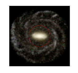
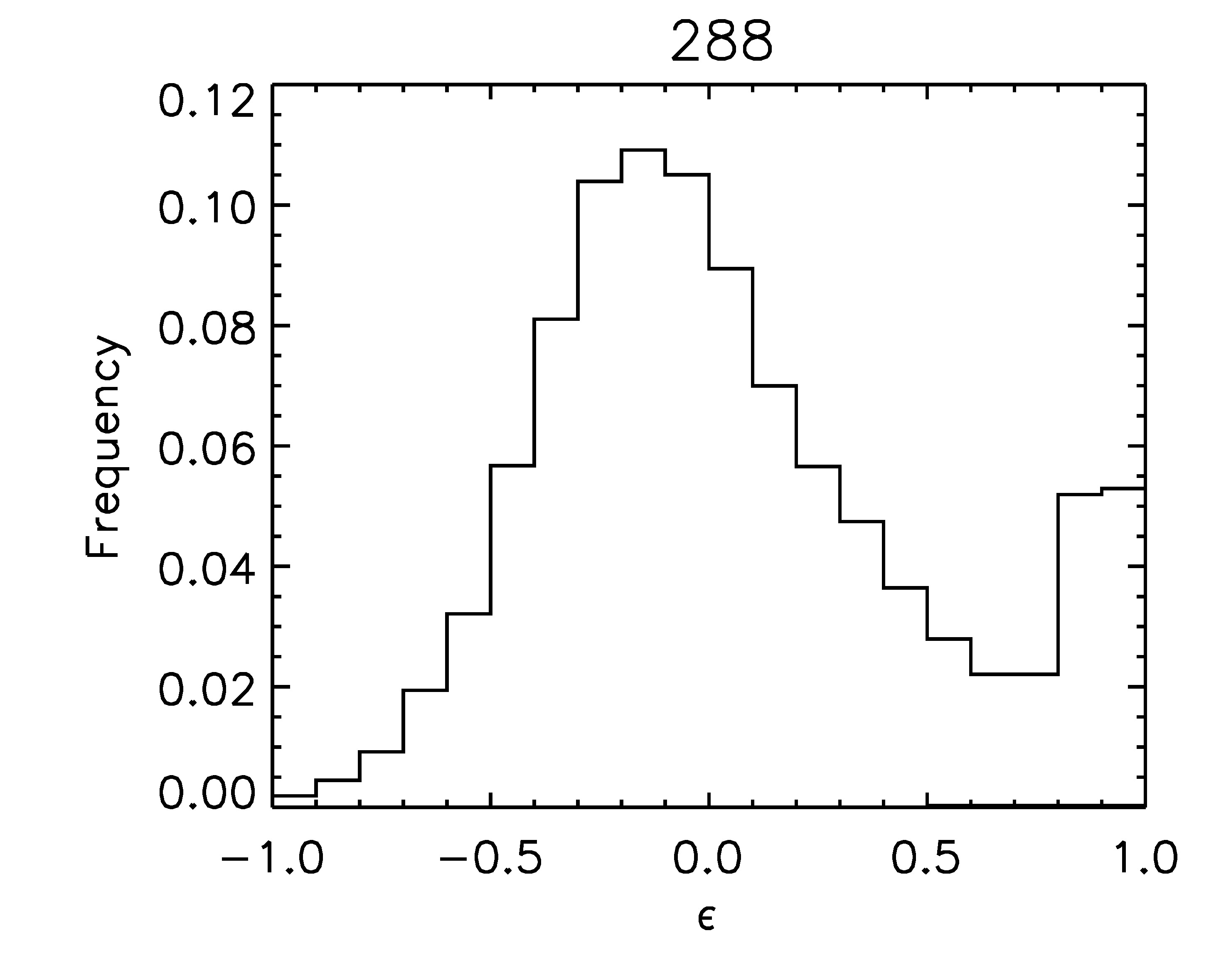
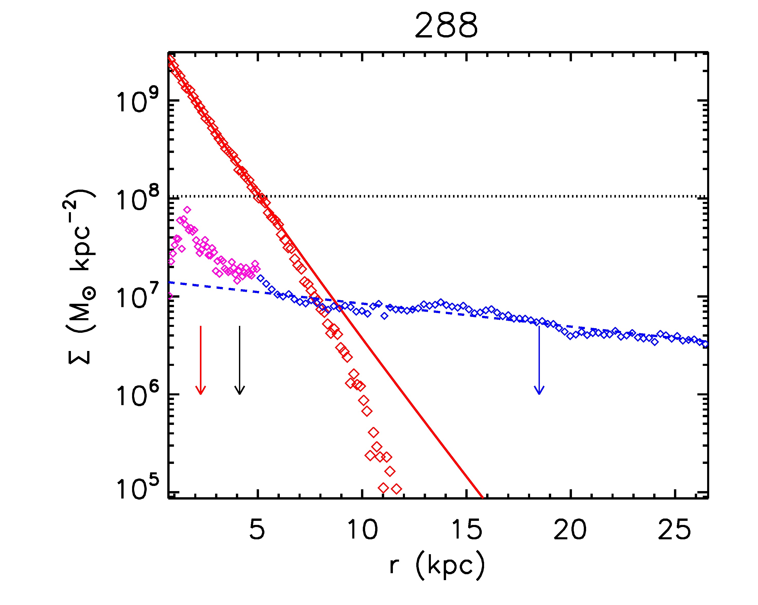
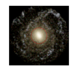
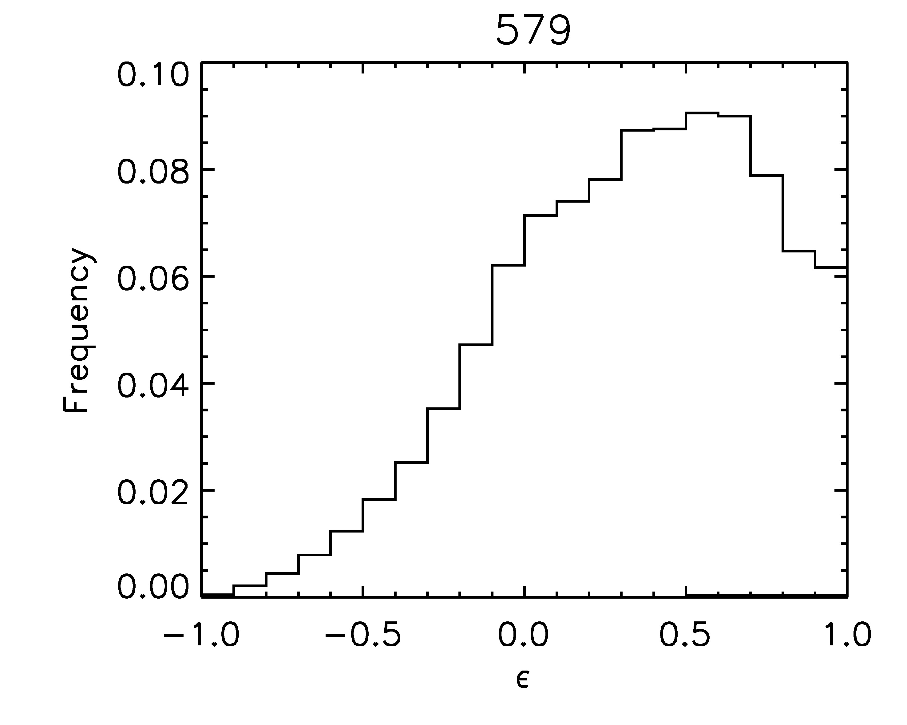
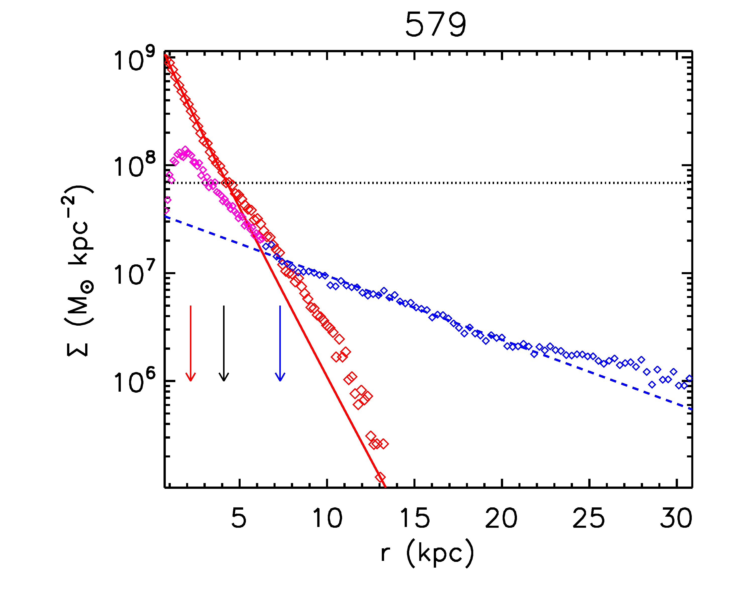
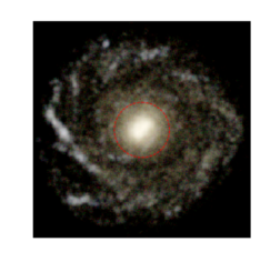
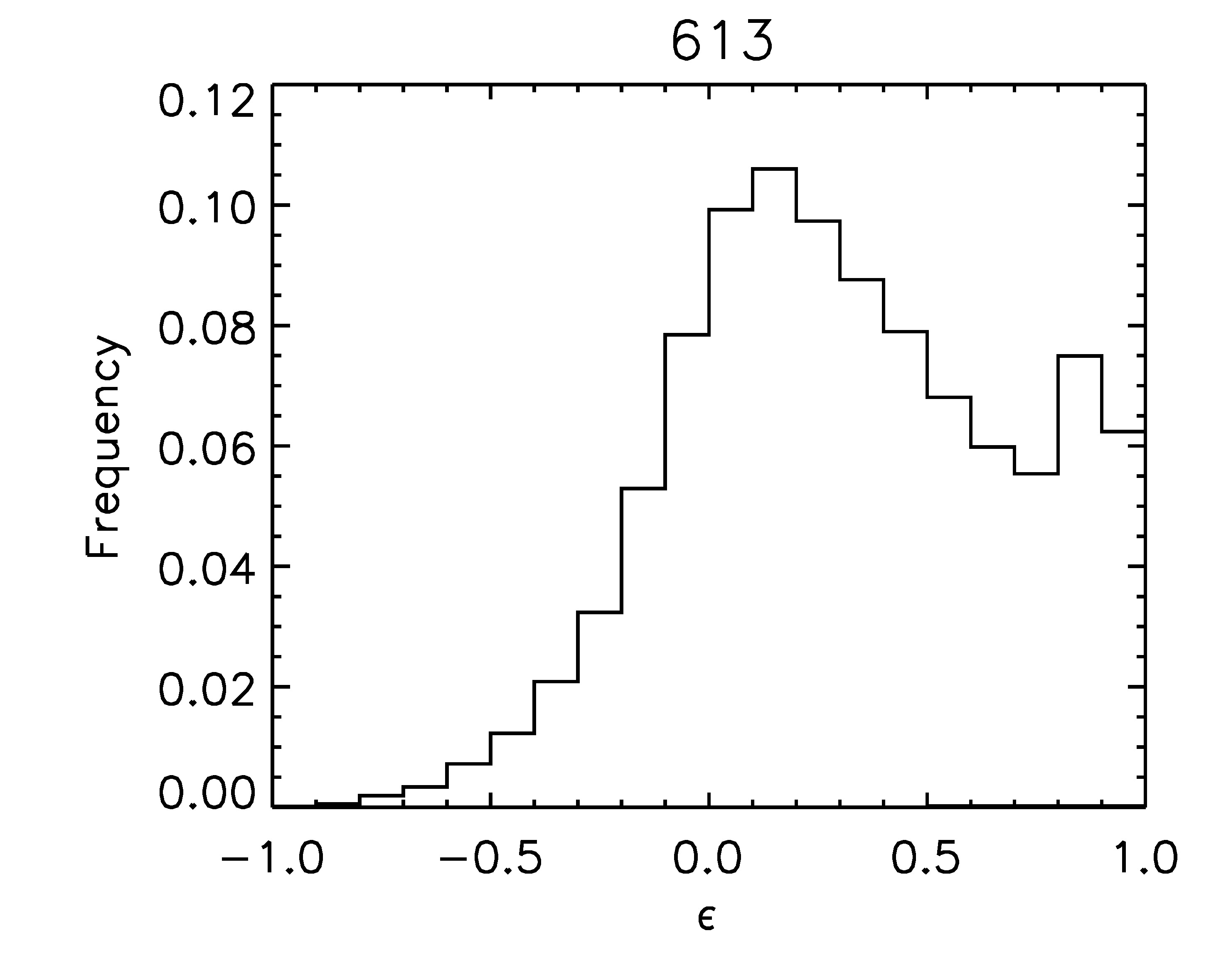
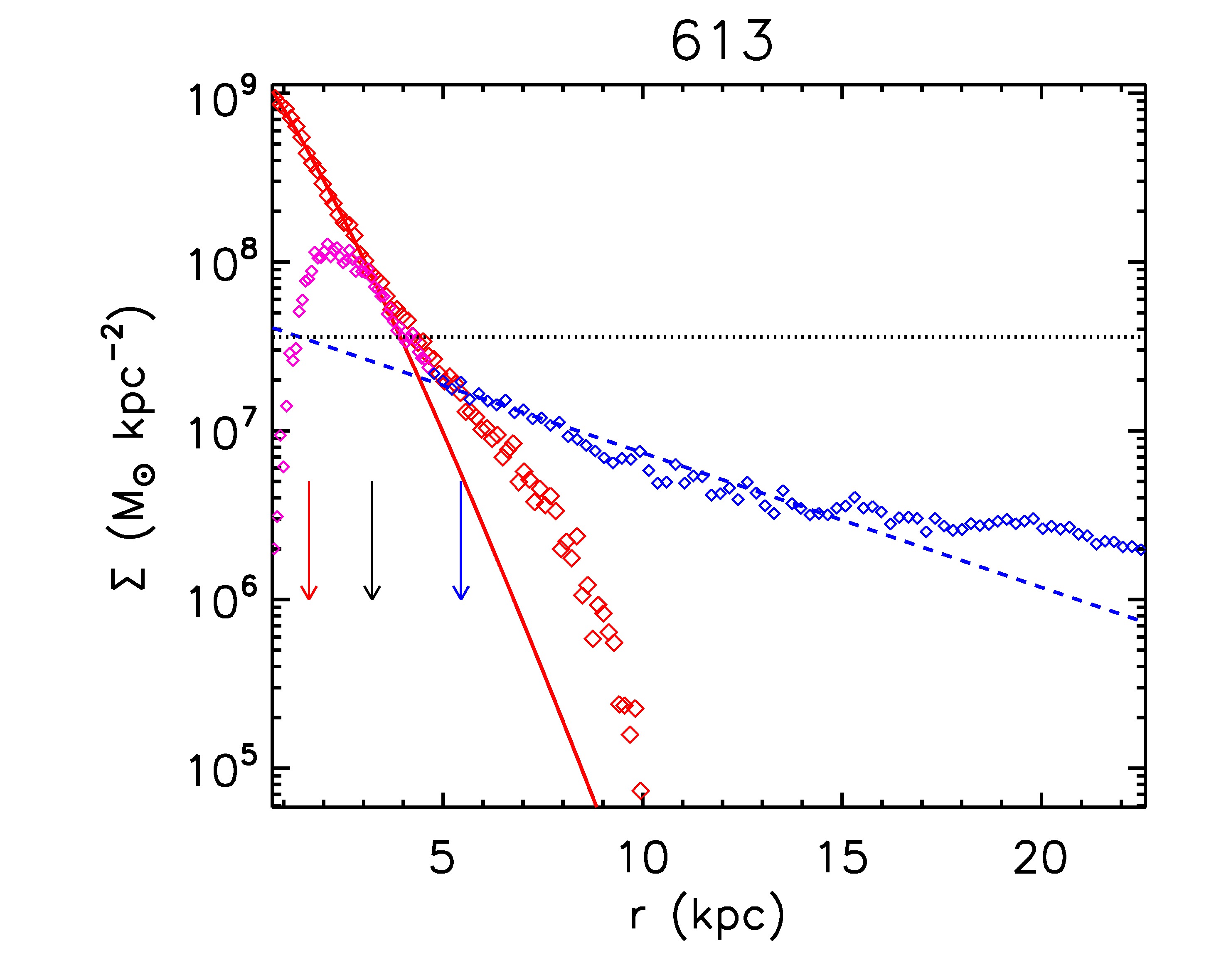
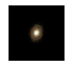
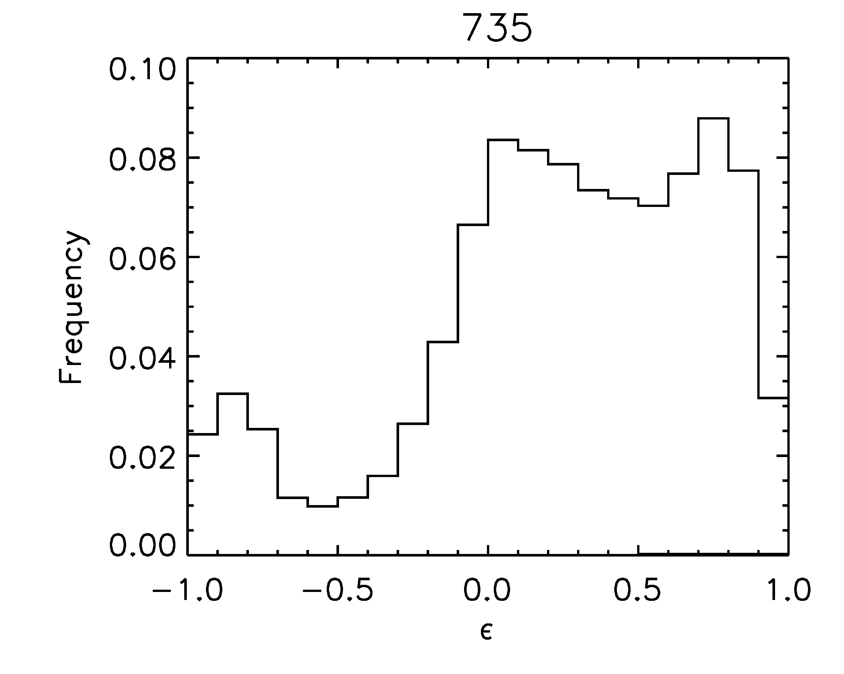
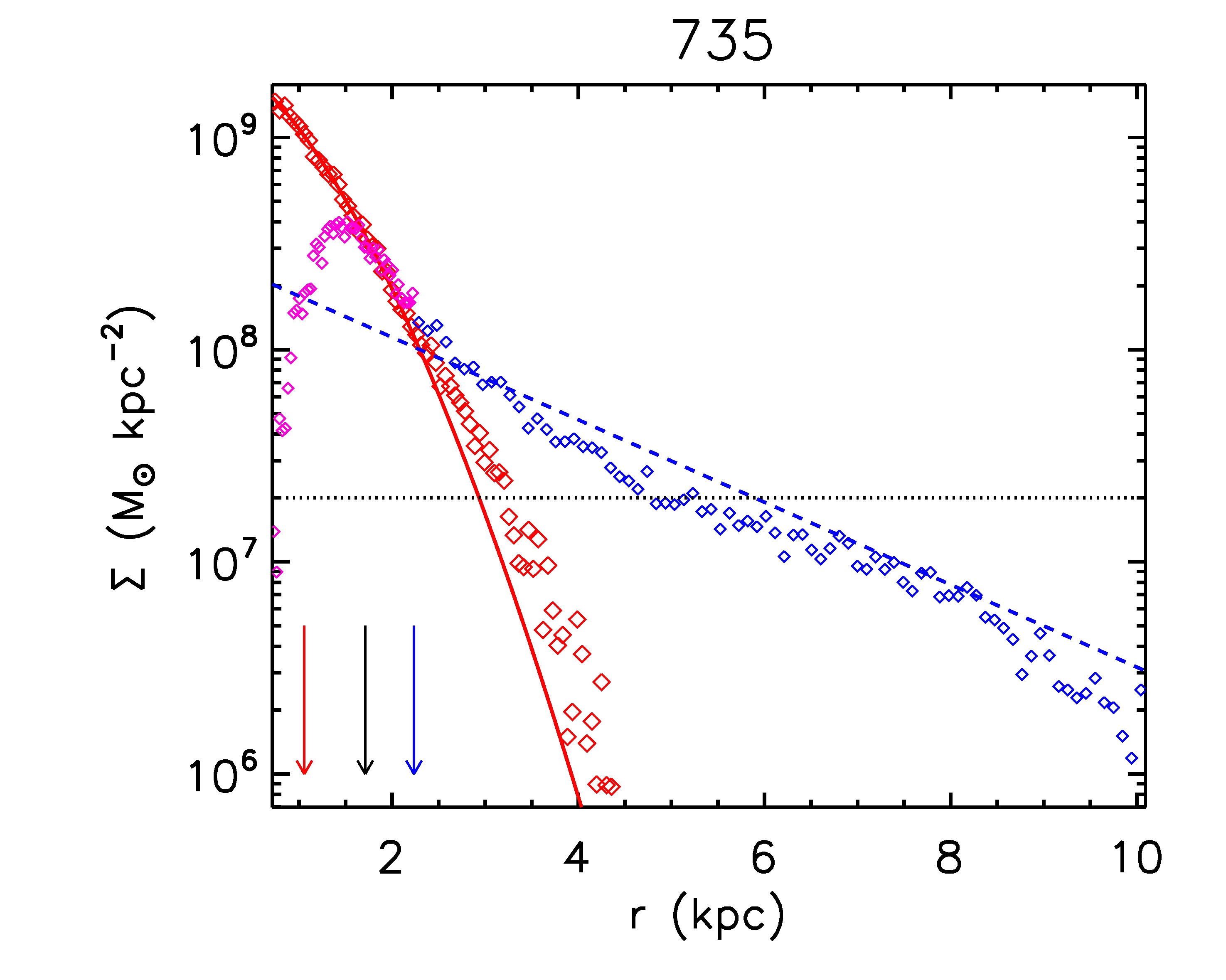
Figure 15: Left panels: Synthetic images of 18 SDGs obtained with the SKIRT code (Baes et al. 2005) with a box side of 30 kpc. The red circles show the limit radii for SDSS observability (see Appendix A for details). Middle panels: Distributions of the $\epsilon$ parameter for star particles within the optical radius. Right panels: Projected stellar-mass surface profiles for the spheroids (red diamonds) and the disc components (blue diamonds). Part of the disc components coexist spatially with the spheroid component (magenta diamonds). The best fit Sersic profile for the spheroid component (red solid lines) and the exponential profiles for the discs (blue dashed lines) are also included. We indicate with a red, black, and blue arrow the $R_{\mathrm{Sersic}}$, $R_{\mathrm{hm}}$, and $R_{d}$ (see Table 1). We also include the total surface brightness at the limit radius where the galaxy could be detected with the SDSS (black dotted line). The relations are shown out to $R_{\mathrm{opt}}$. The rows show galaxies in order of descending stellar mass. The galaxy ID is indicated above each middle and right panel.

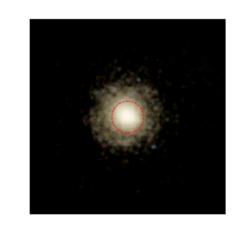
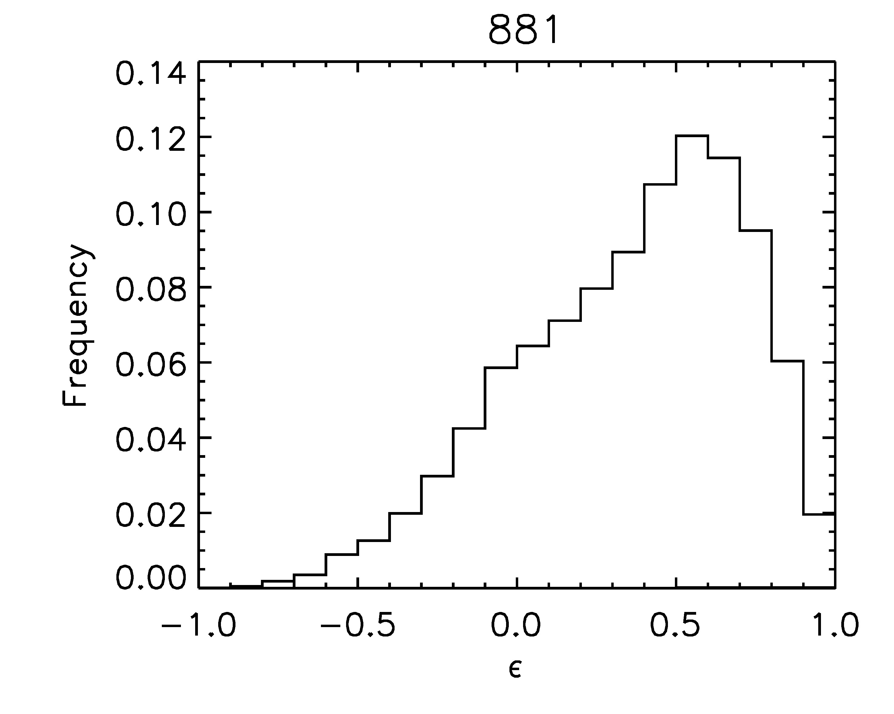
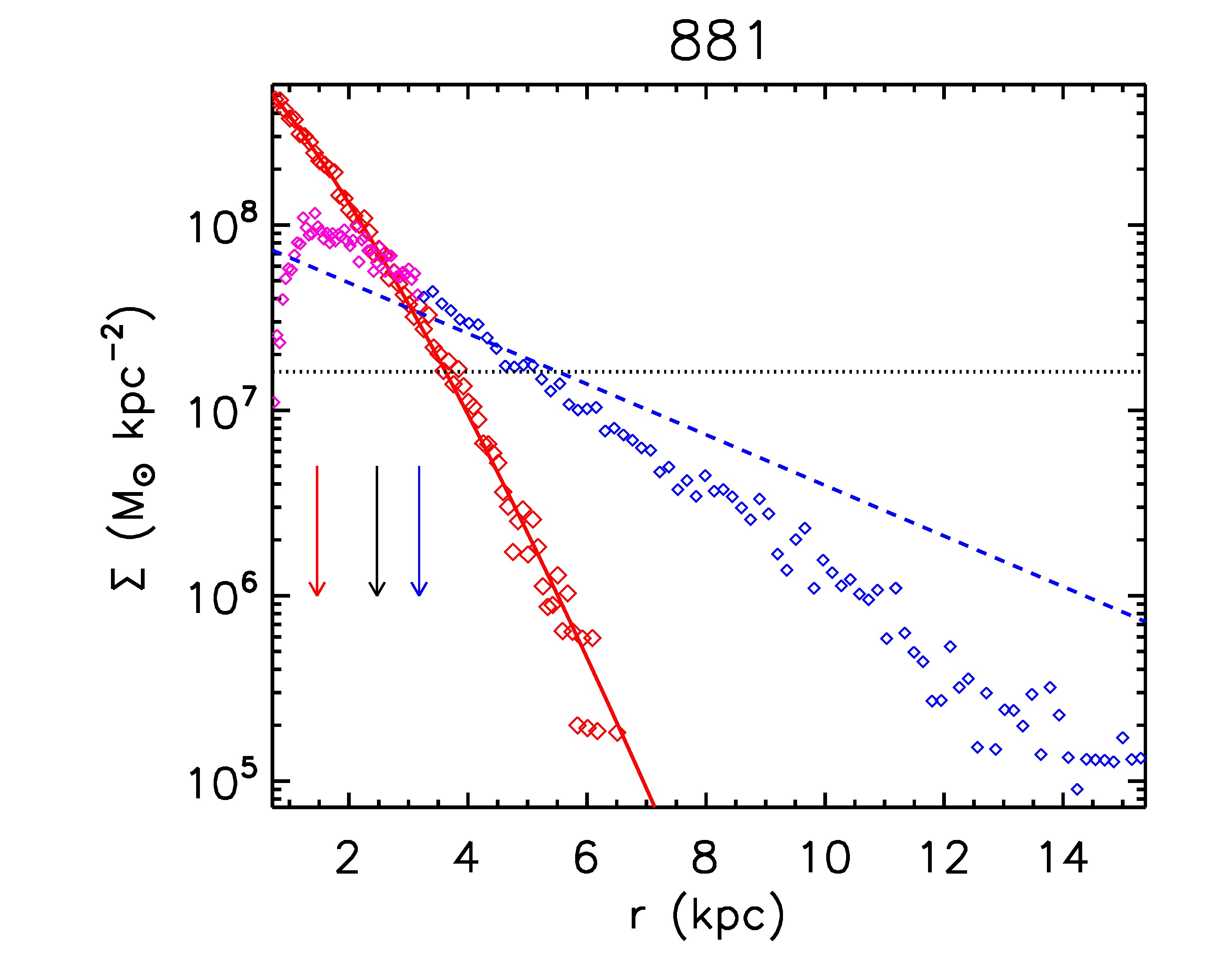
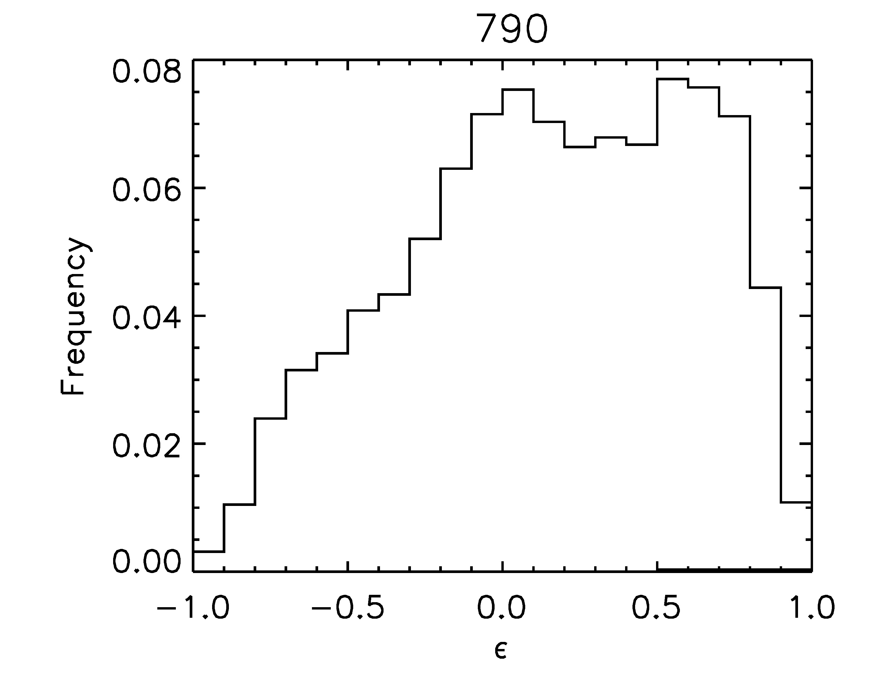
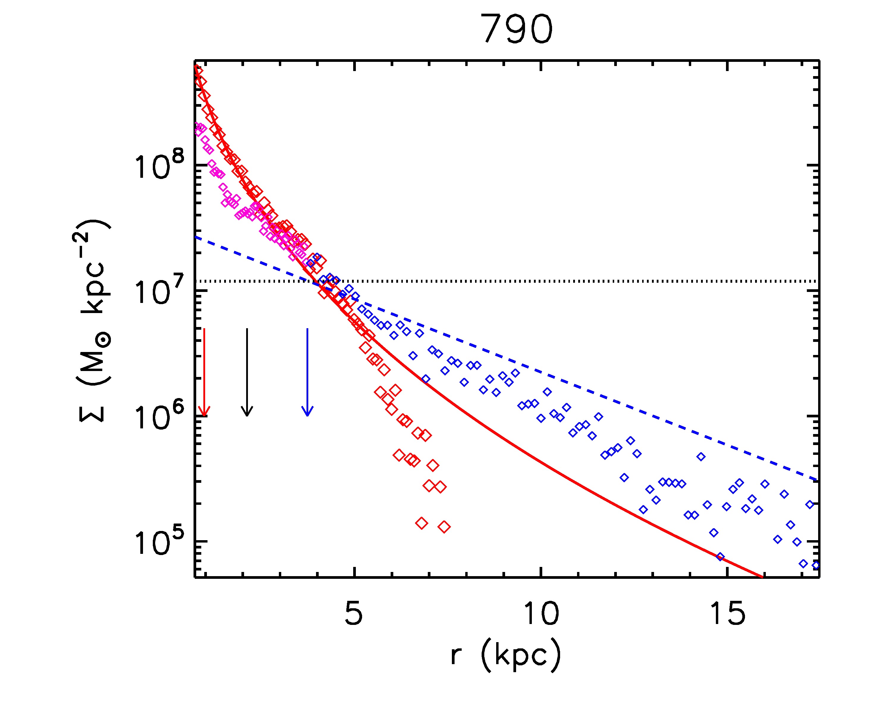
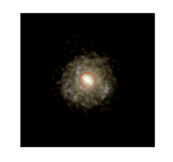
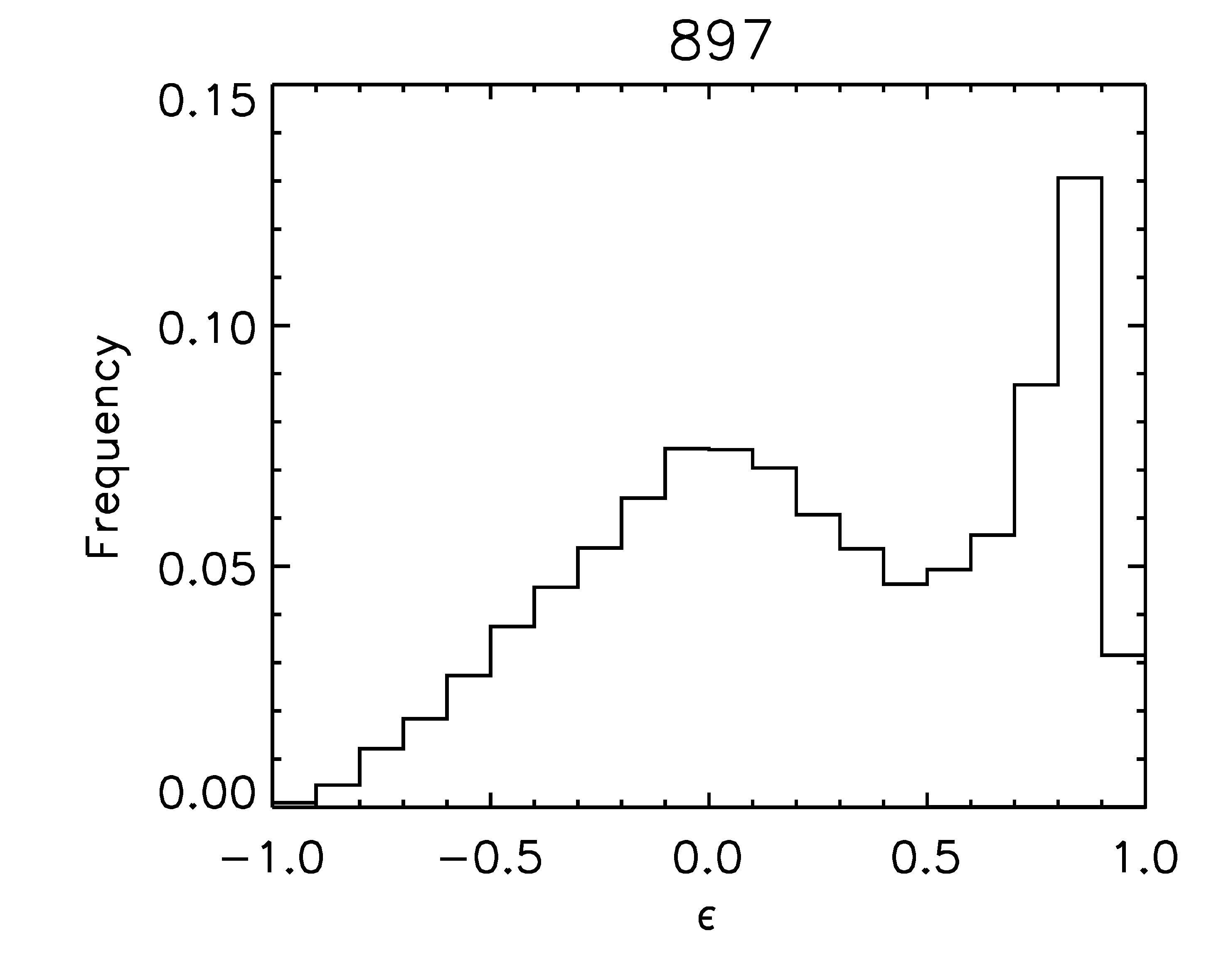
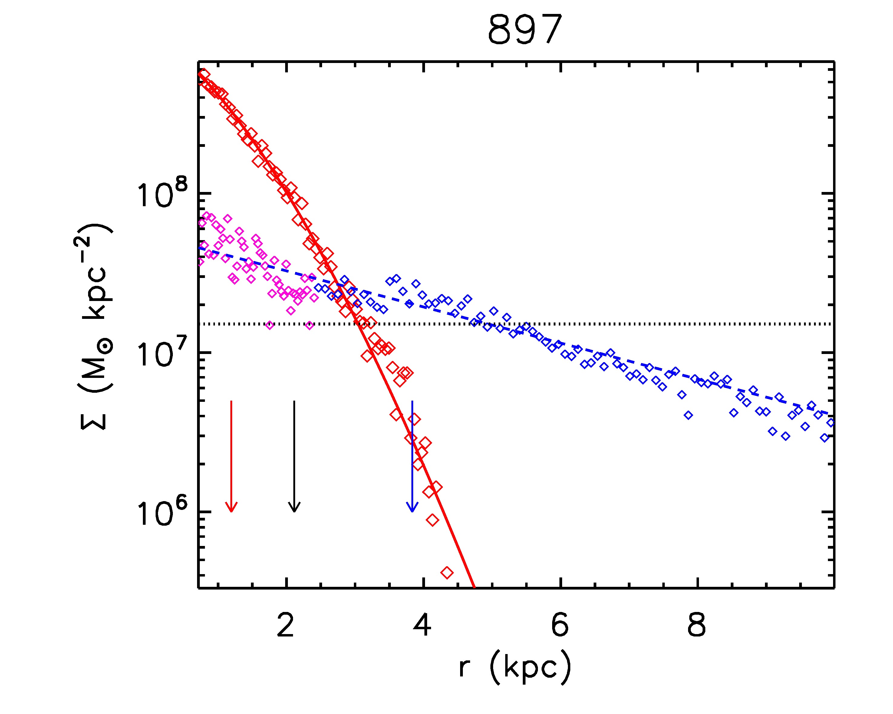
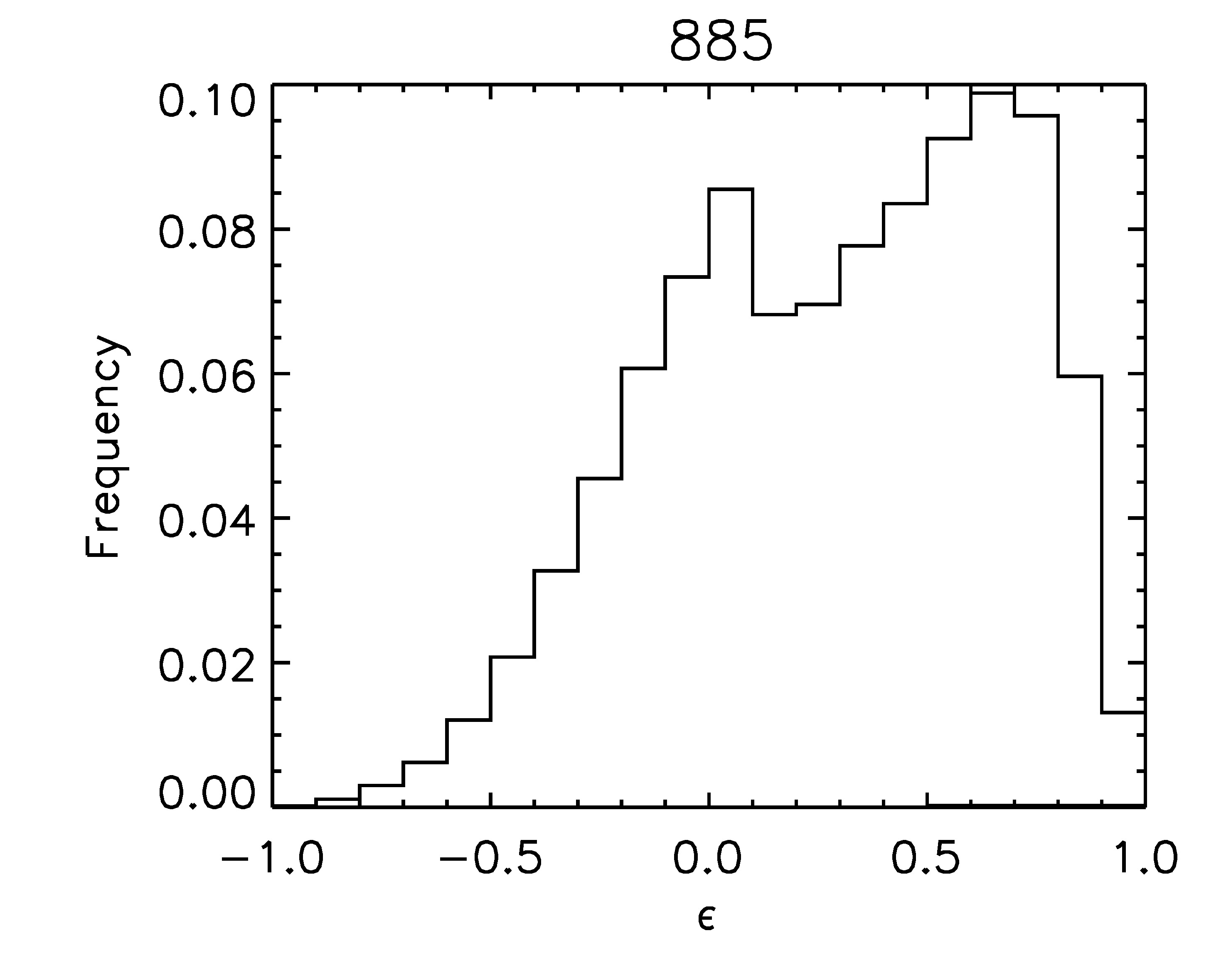
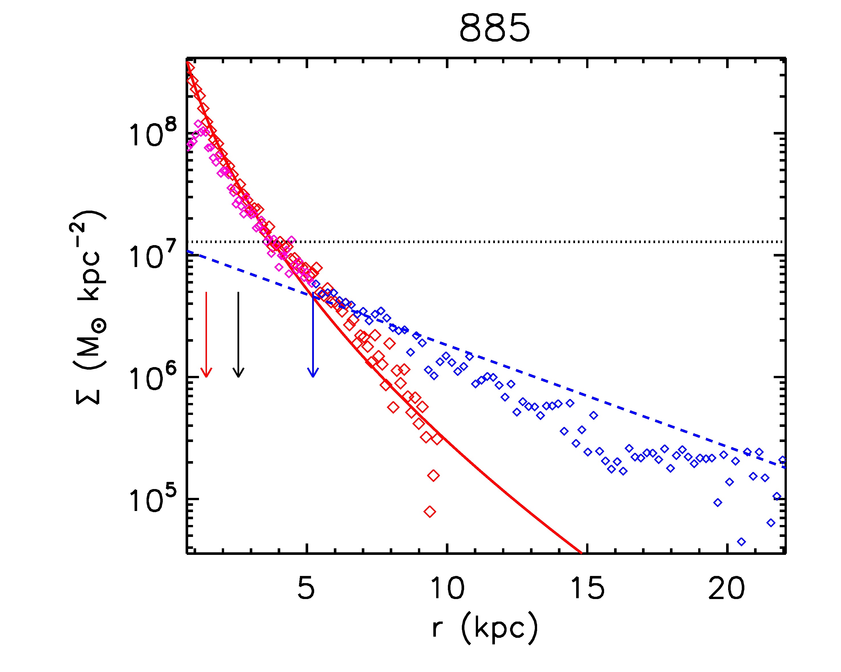
Figure 15: (continued)

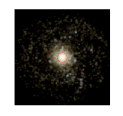
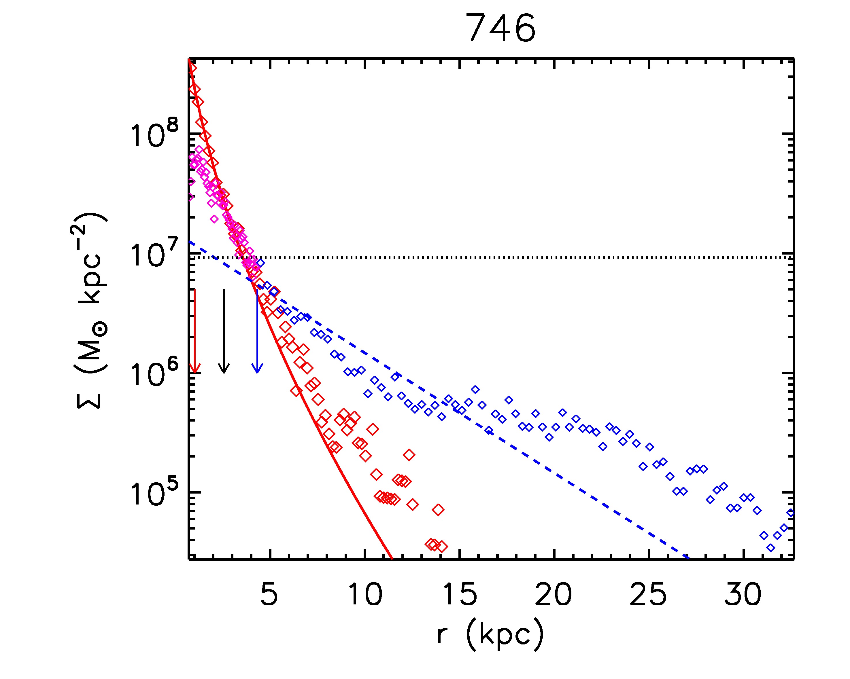
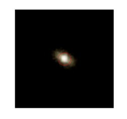
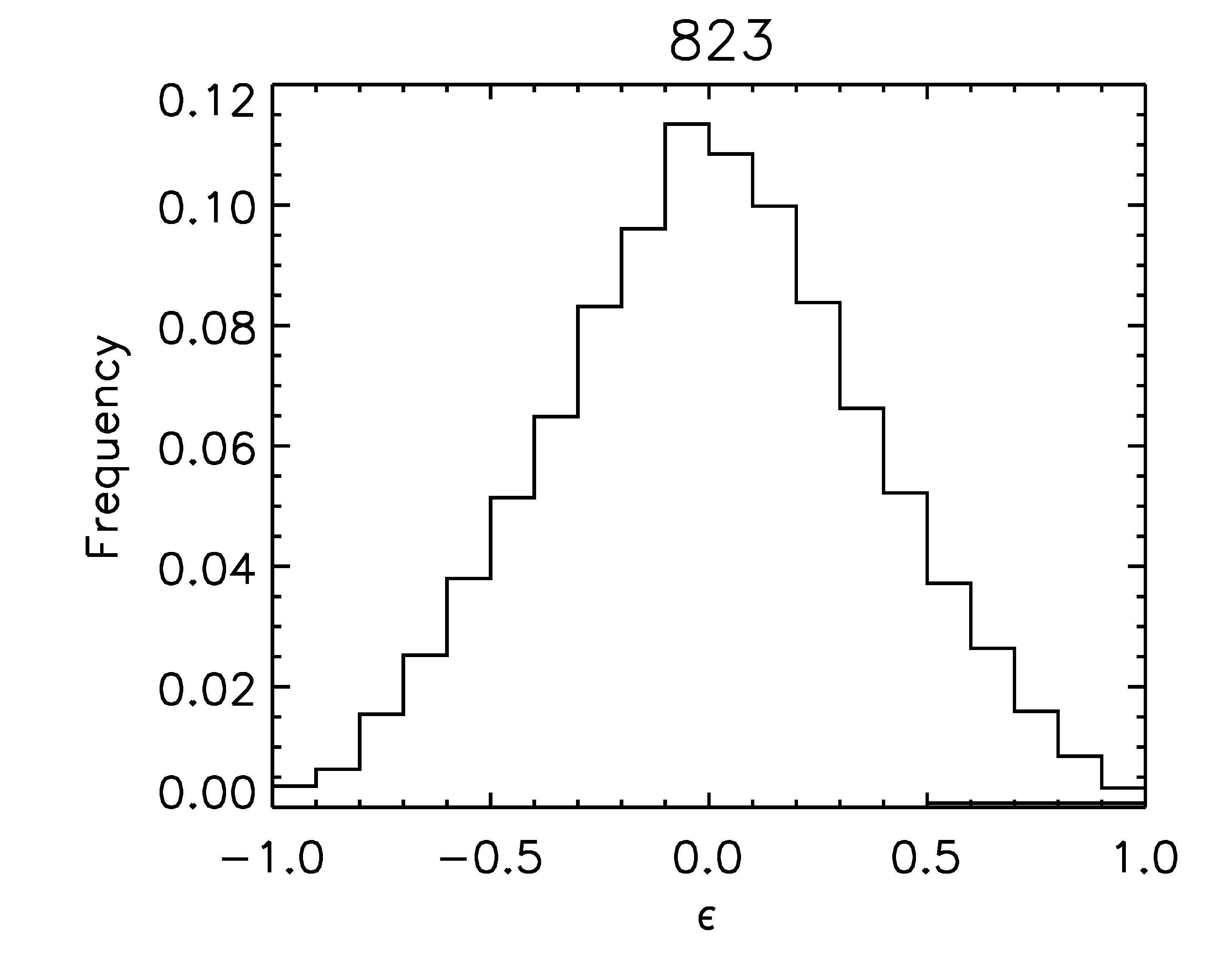
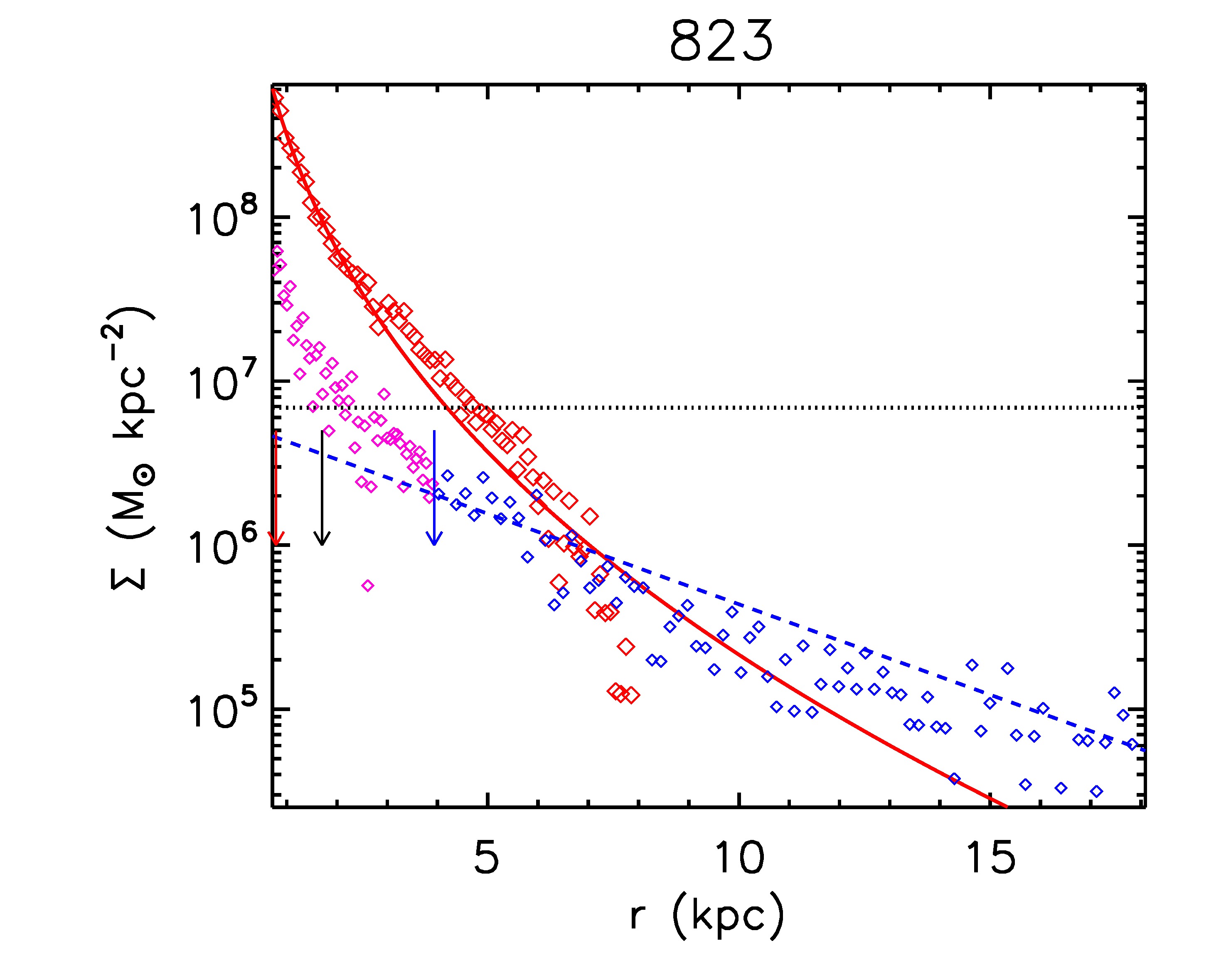
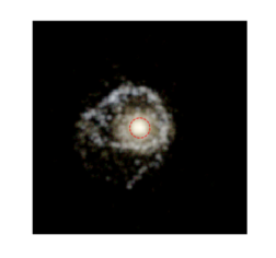
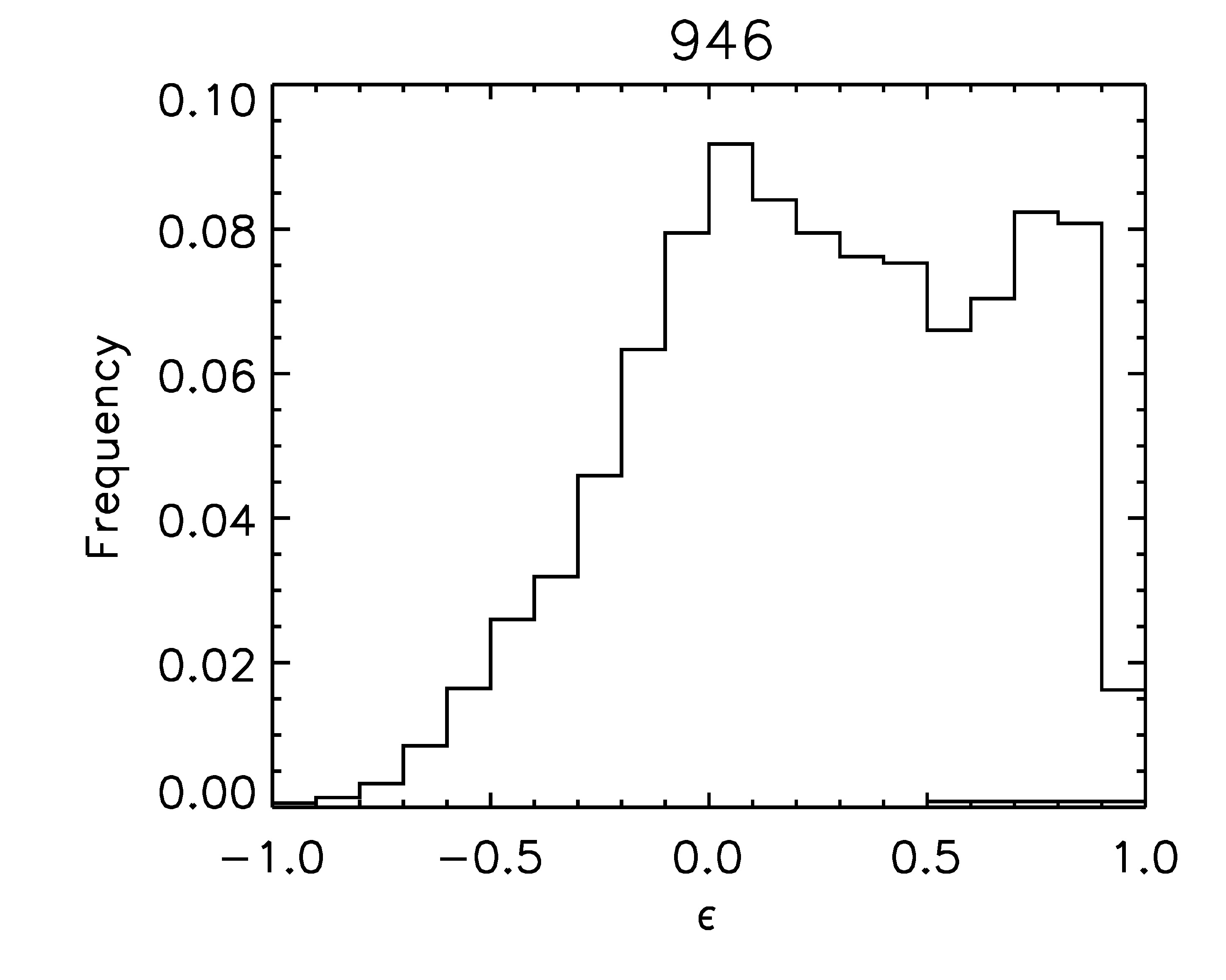
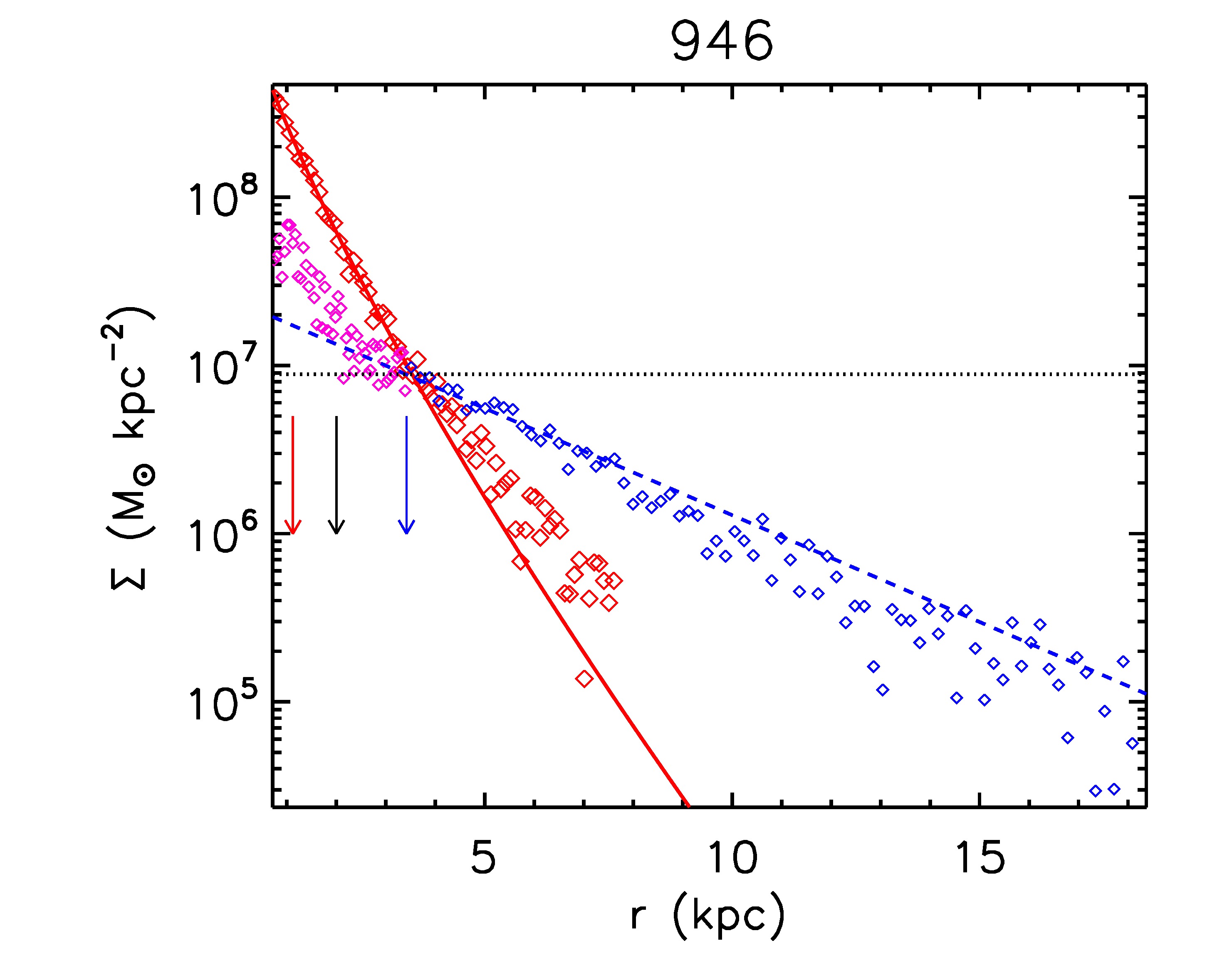
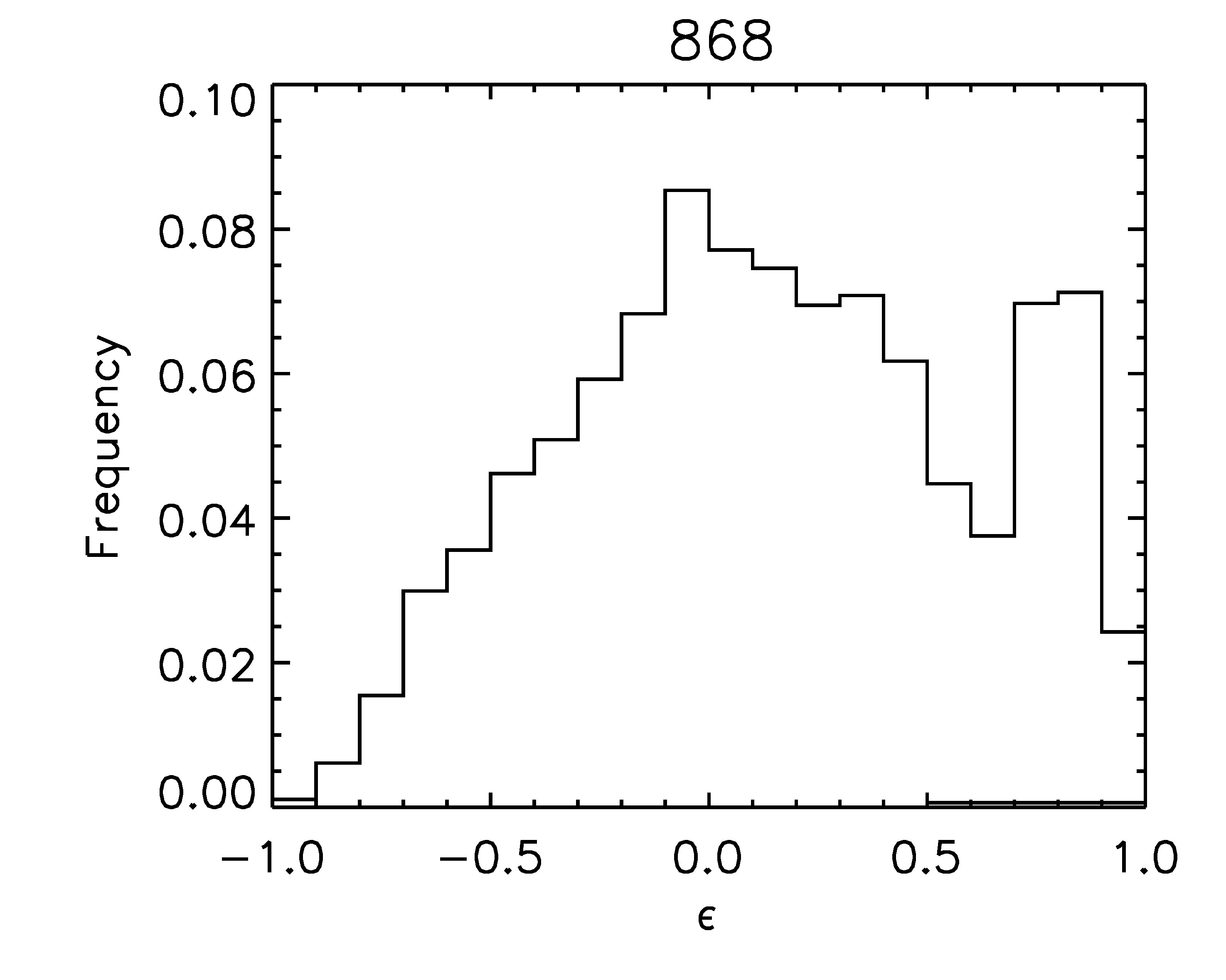
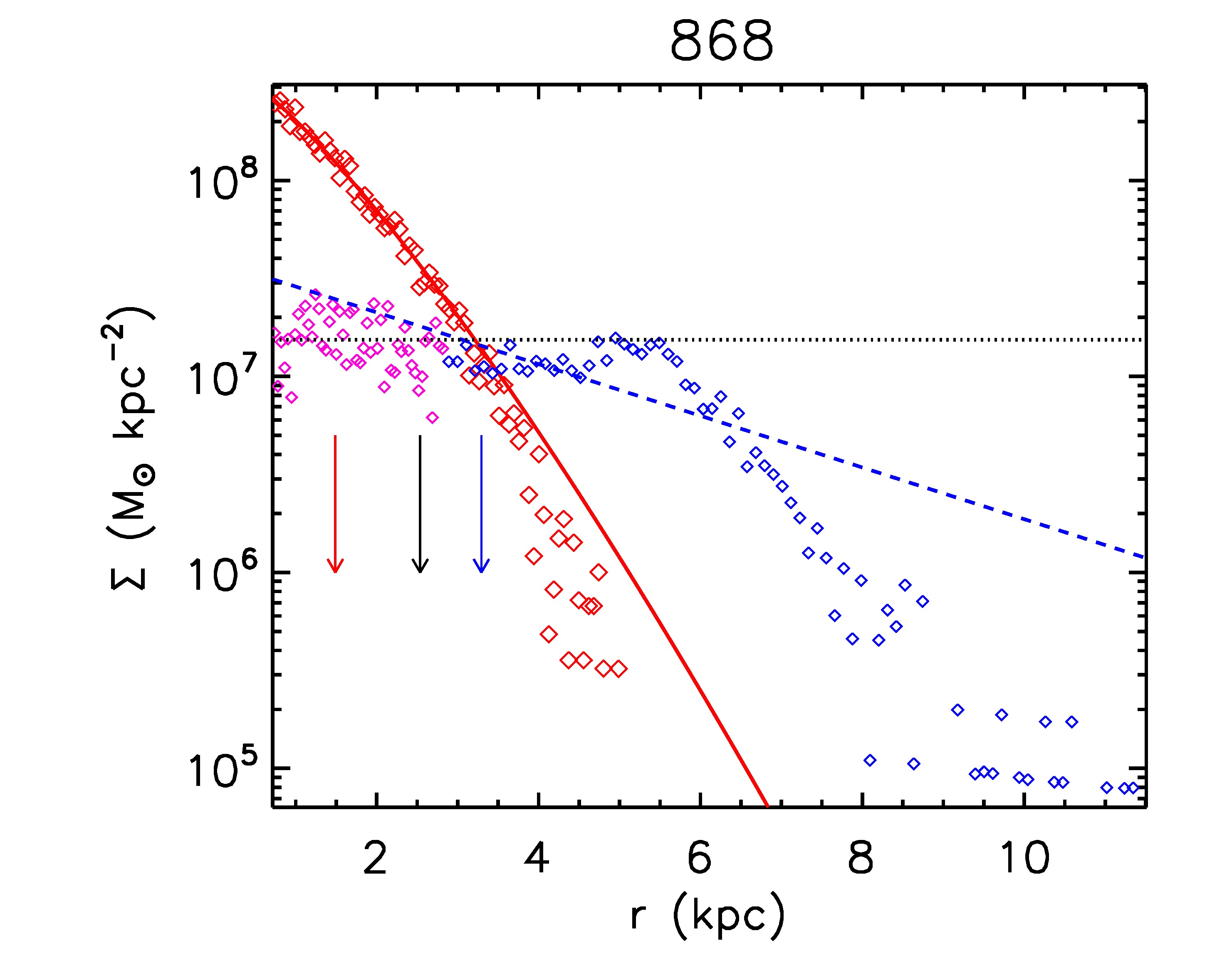
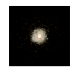
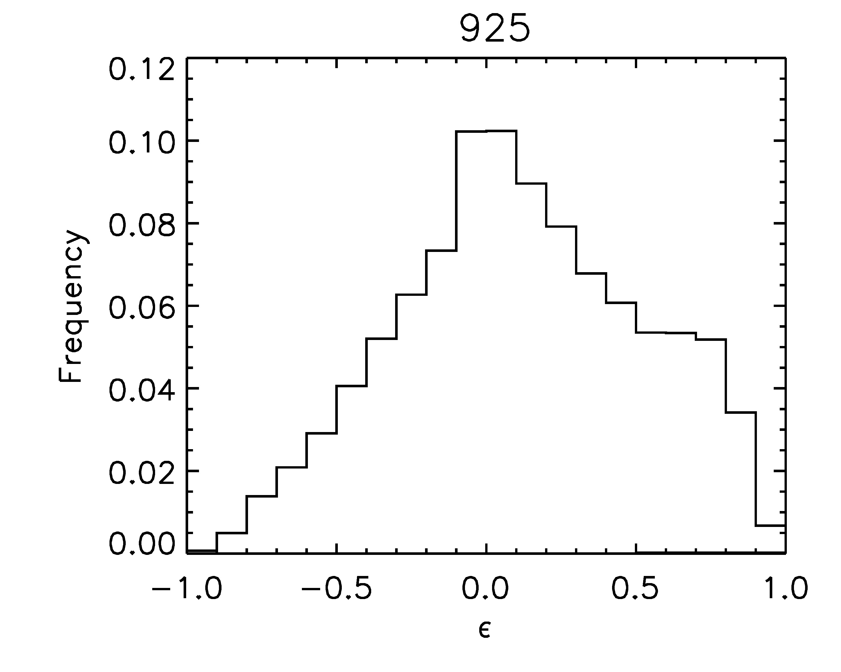
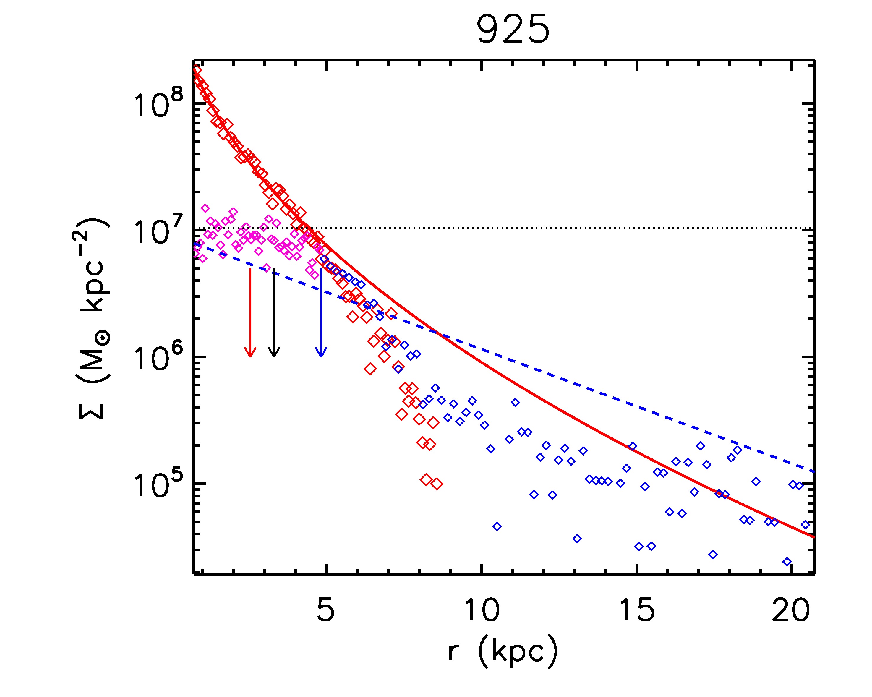
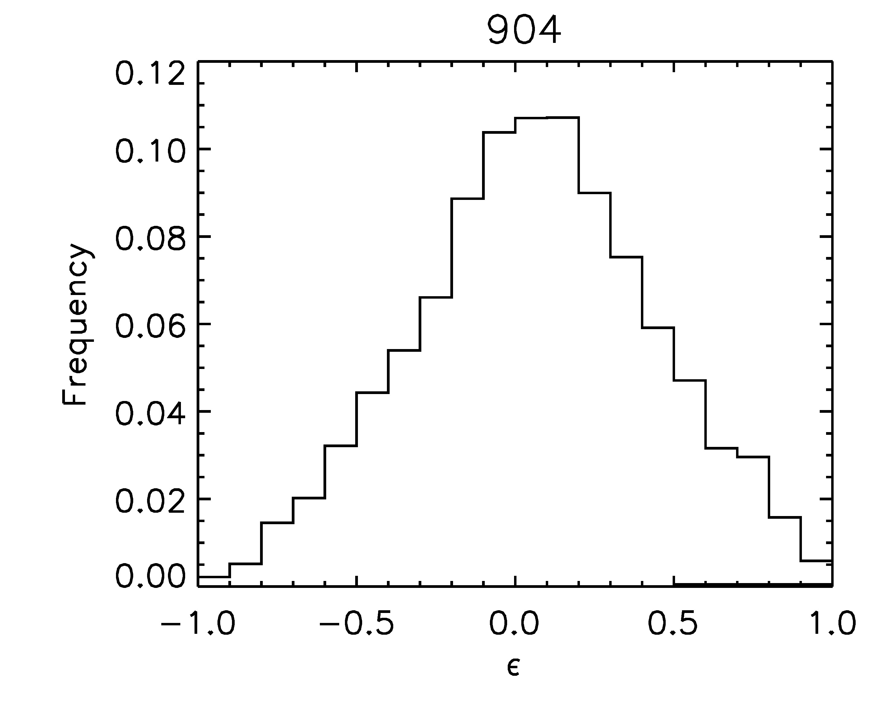
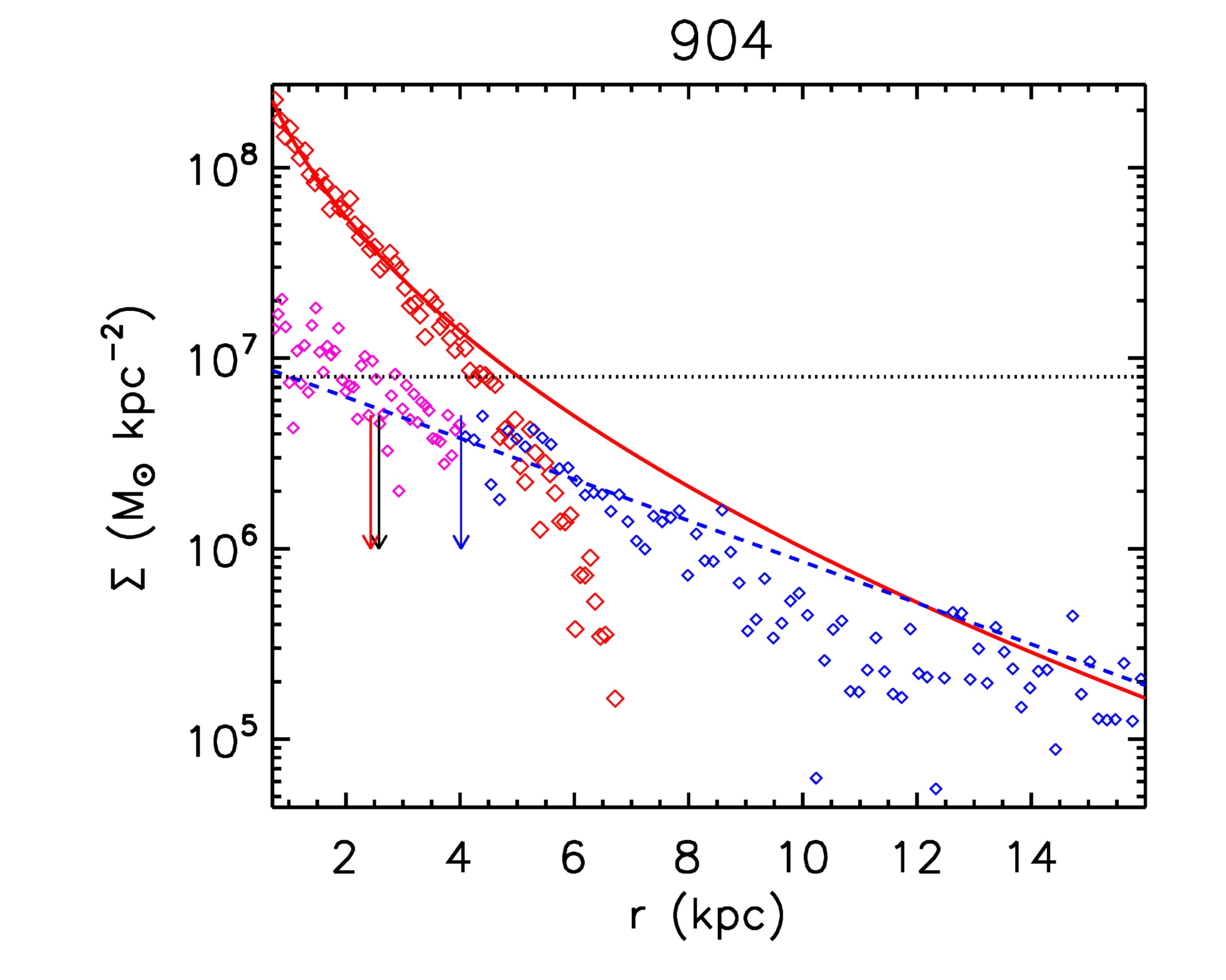
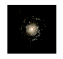
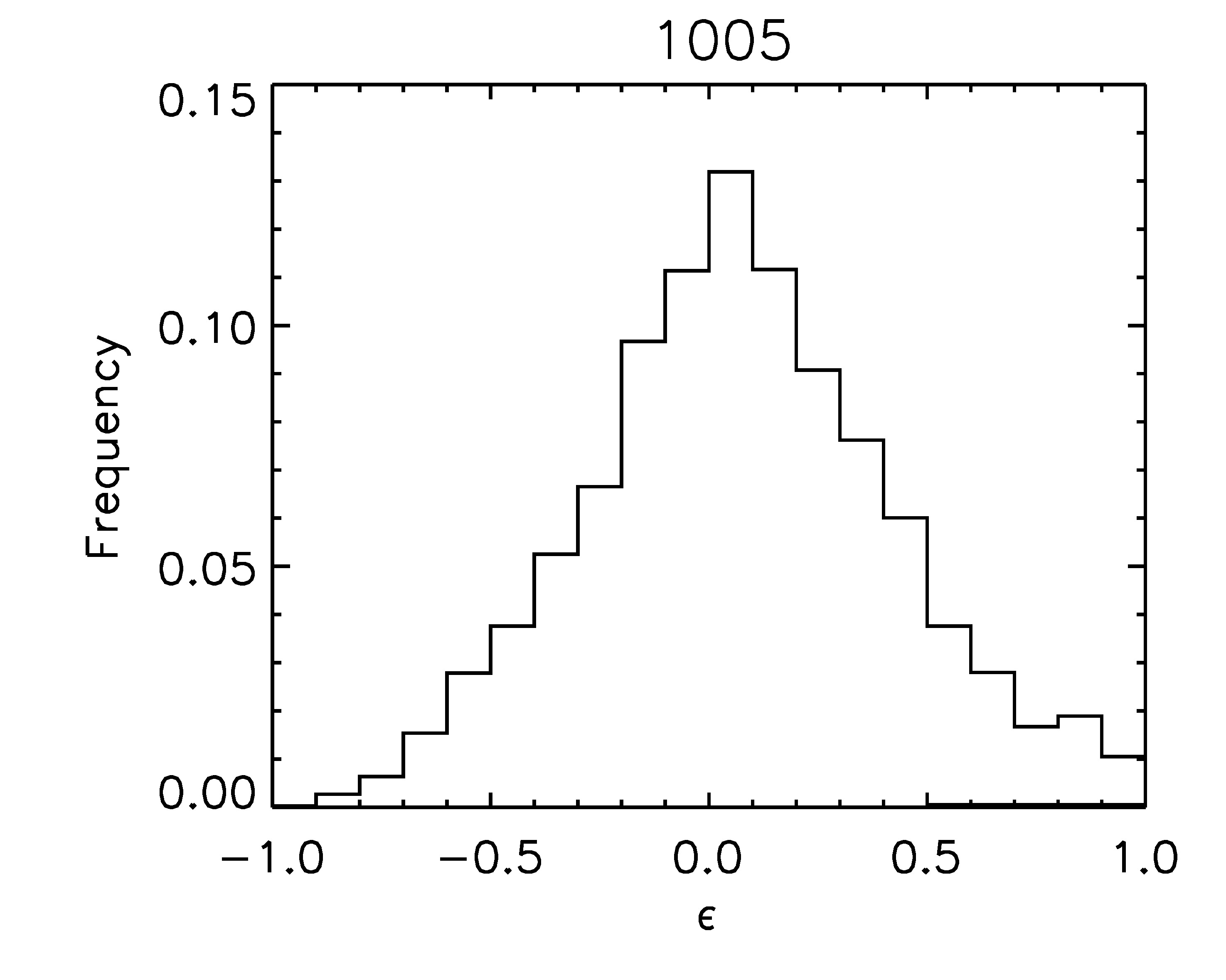
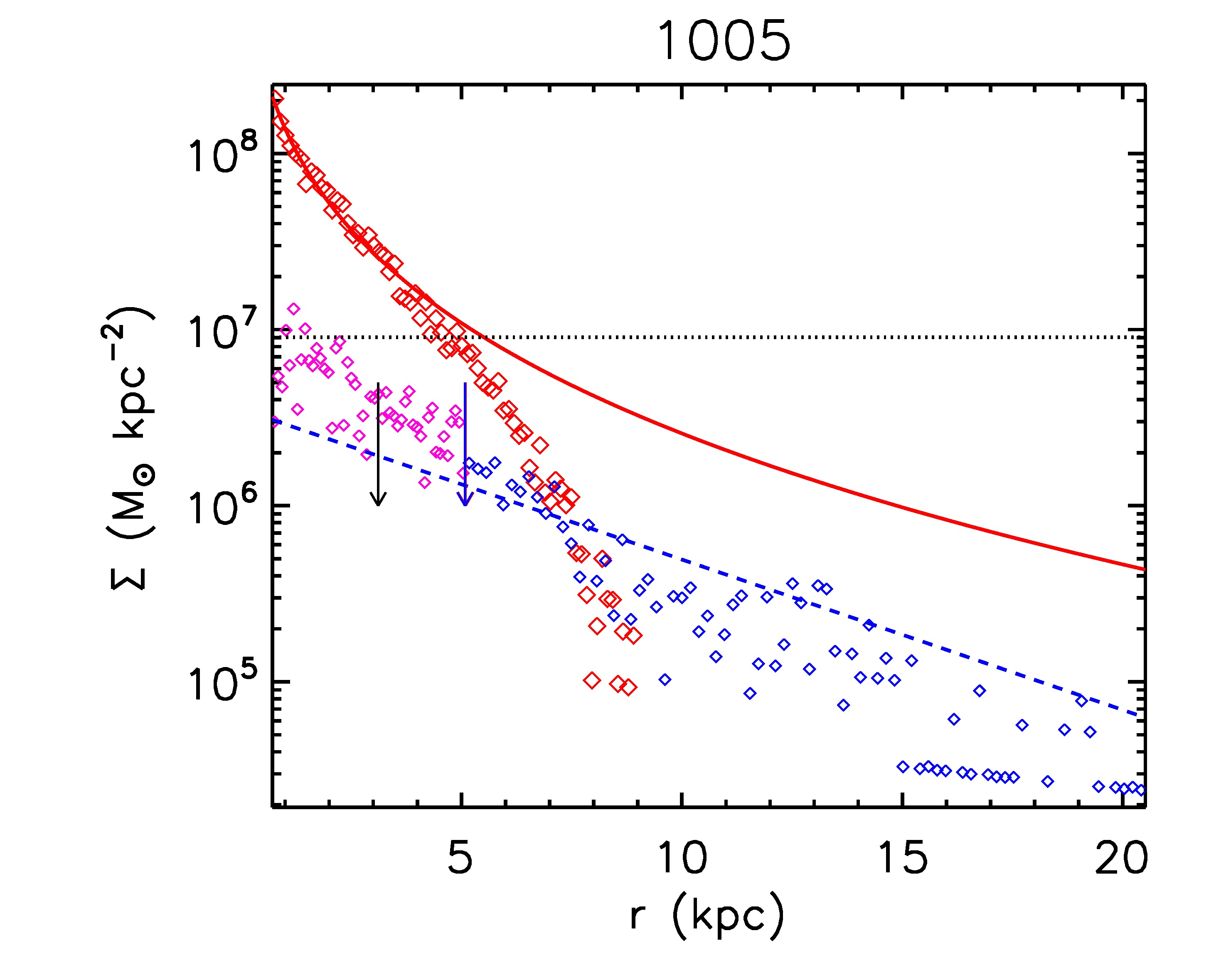
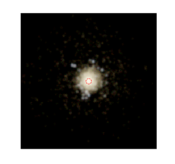
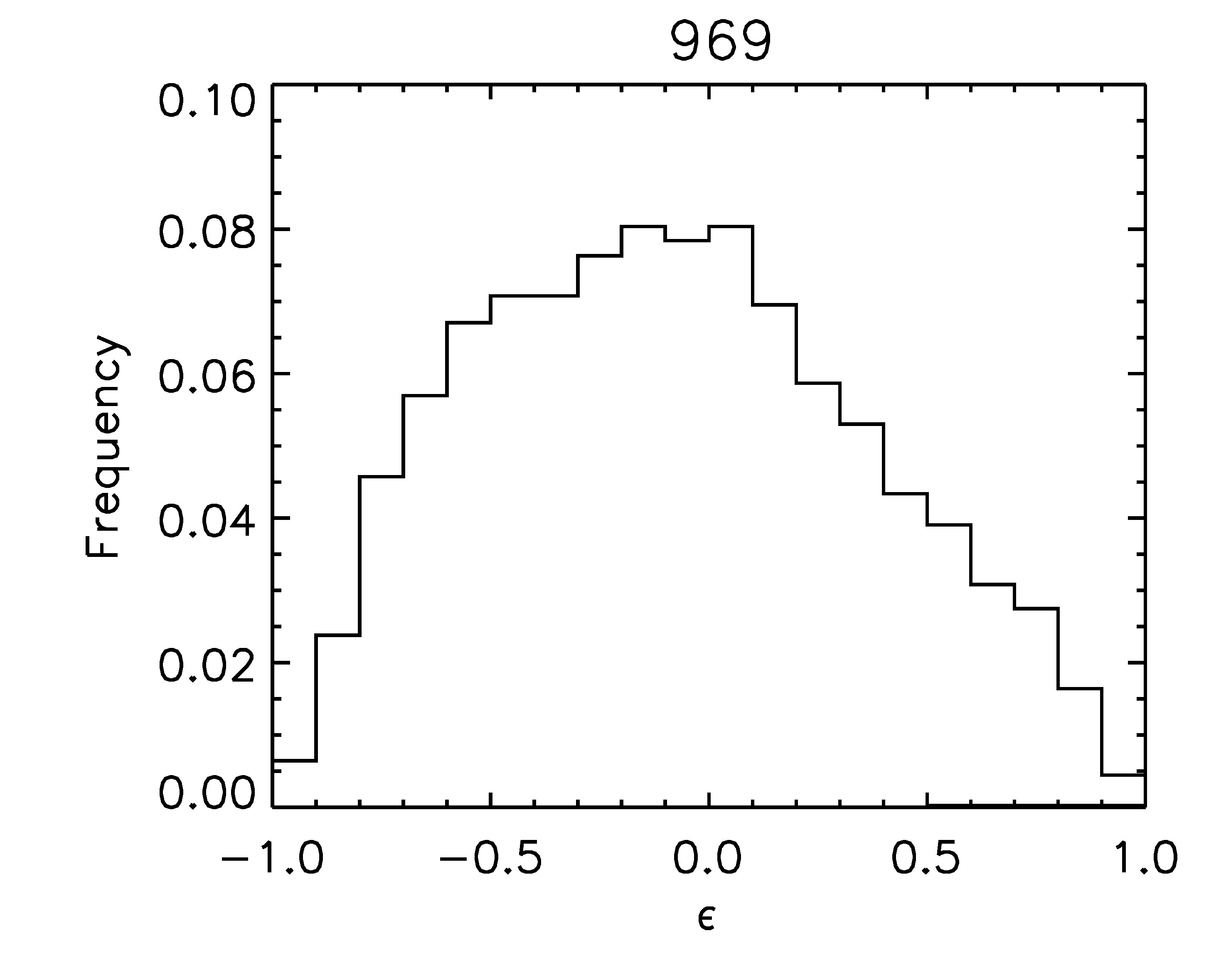
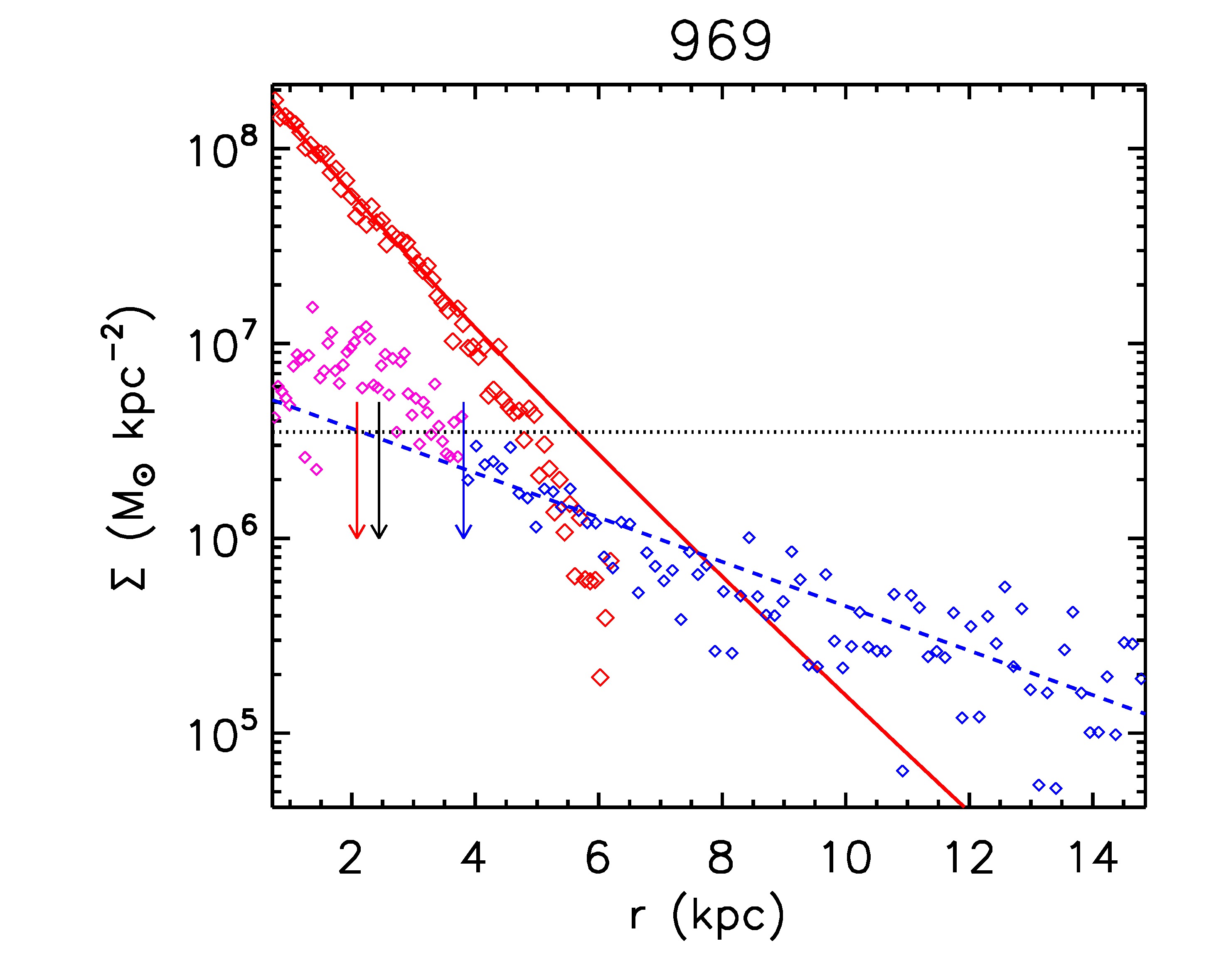
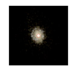
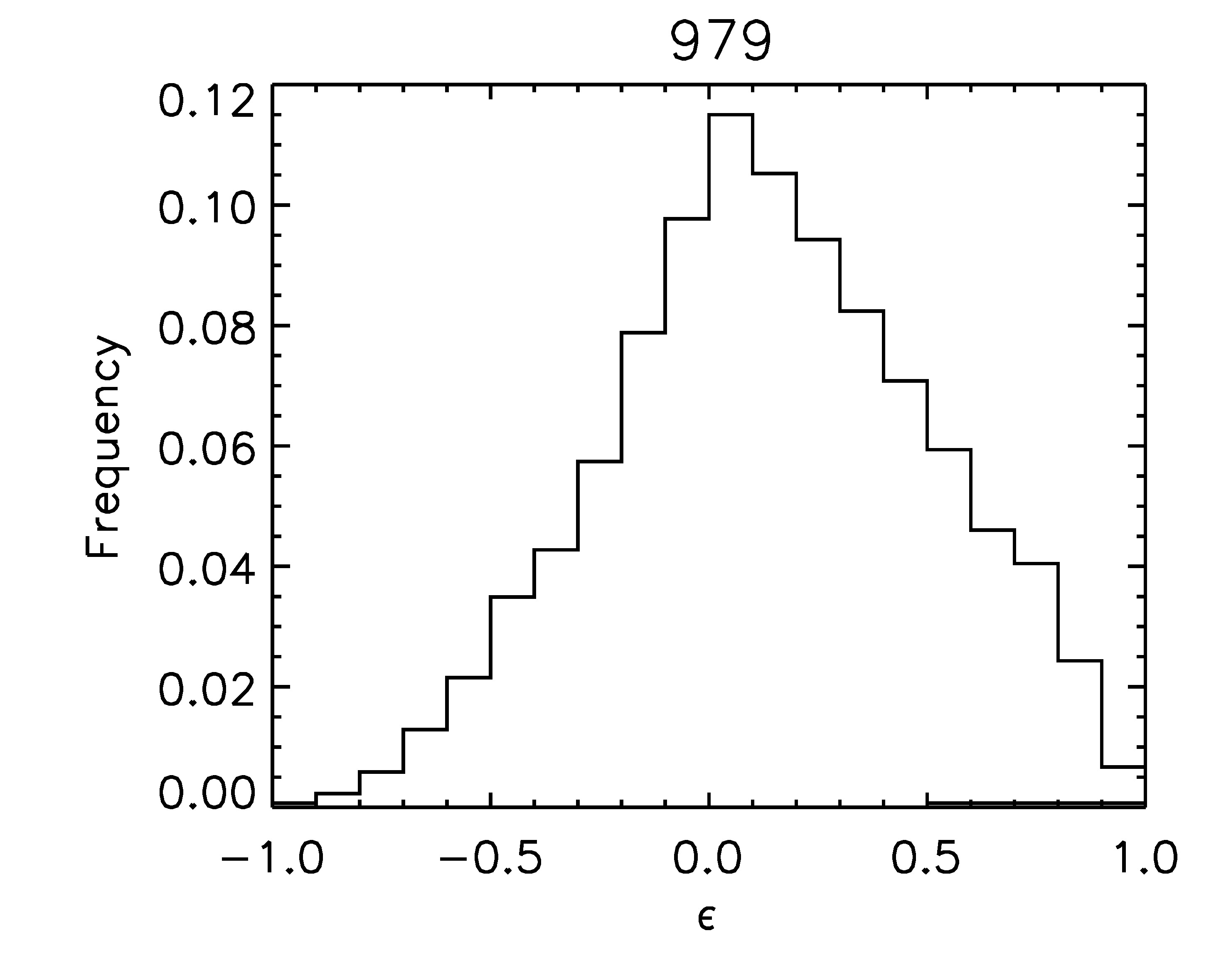
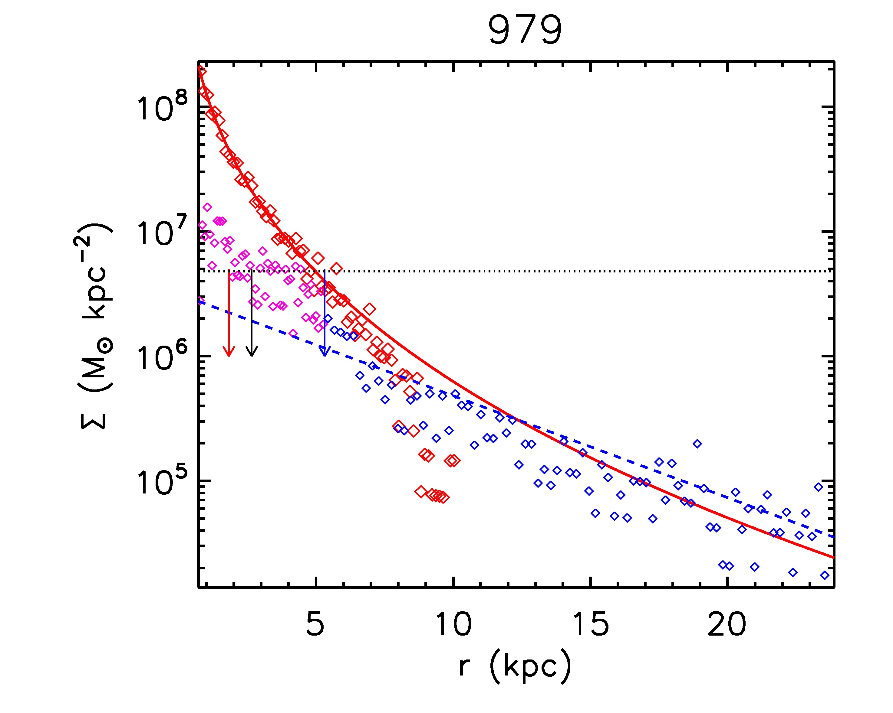
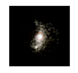
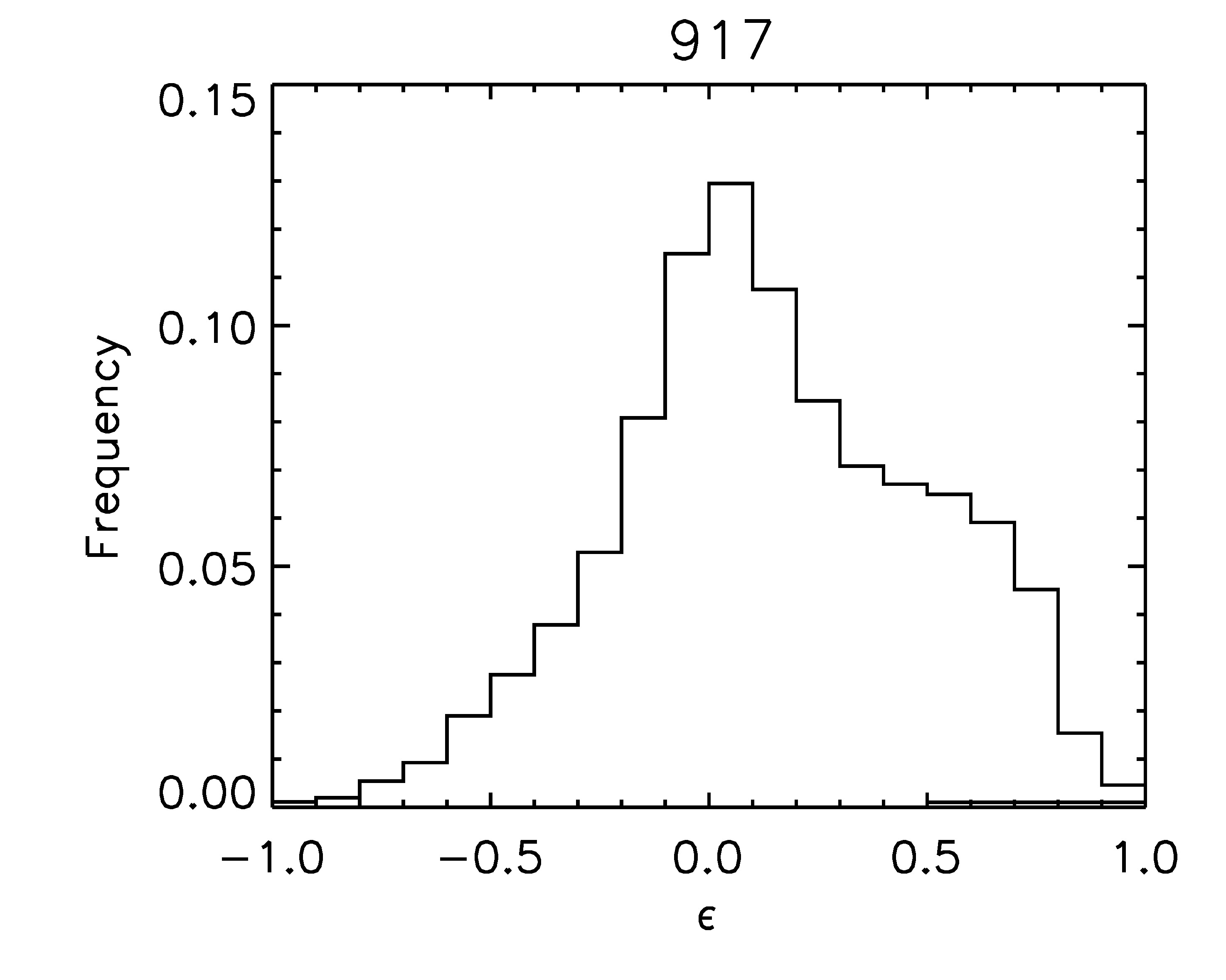
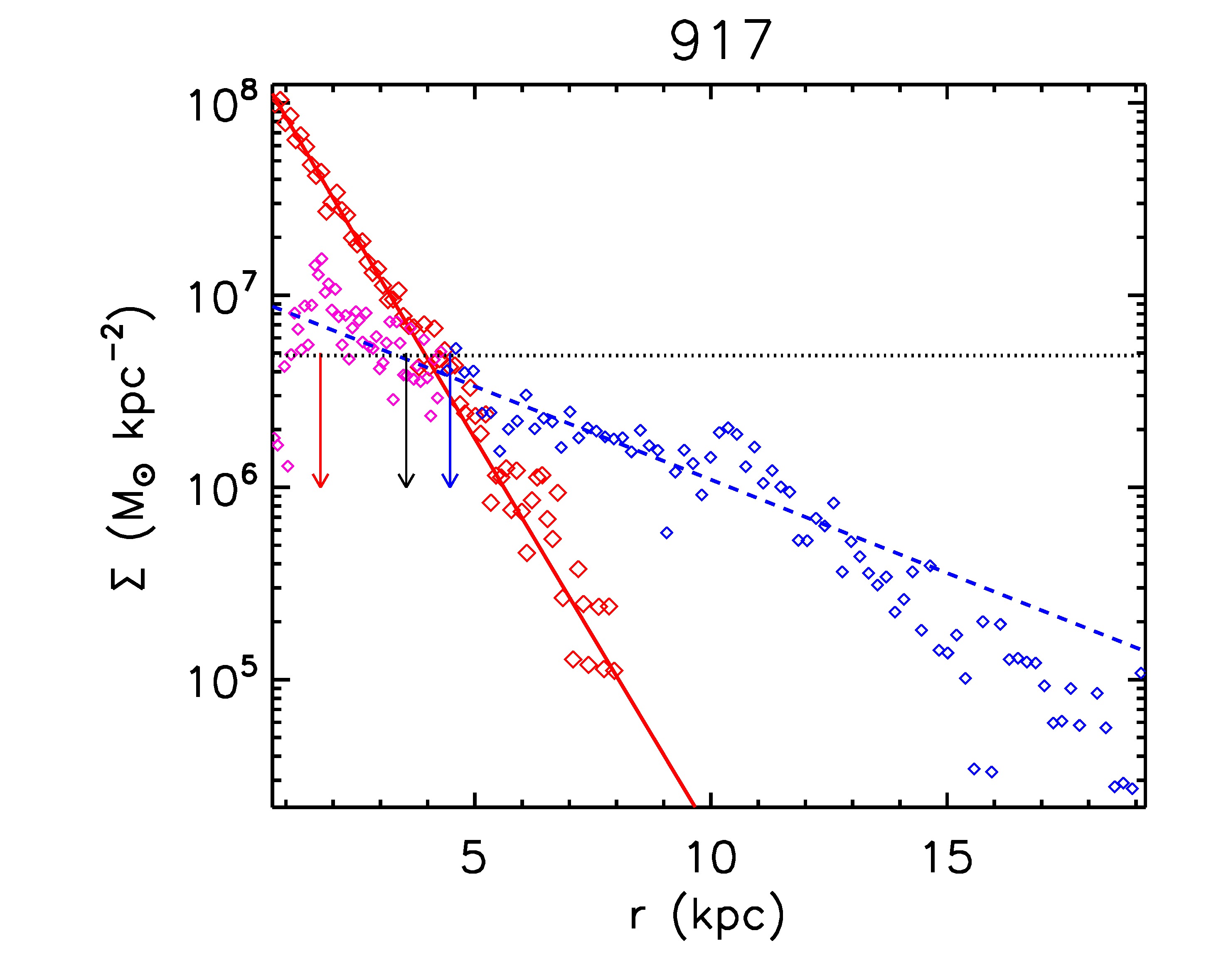
Figure 15: (continued)

Figure 15: (continued)

Figure 15: (continued)