Sparse Tensor Algebra Optimizations with Workspaces

Abstract.

This paper shows how to optimize sparse tensor algebraic expressions by introducing temporary tensors, called workspaces, into the resulting loop nests. We develop a new intermediate language for tensor operations called concrete index notation that extends tensor index notation. Concrete index notation expresses when and where sub-computations occur and what tensor they are stored into. We then describe the workspace optimization in this language, and how to compile it to sparse code by building on prior work in the literature.

We demonstrate the importance of the optimization on several important sparse tensor kernels, including sparse matrix-matrix multiplication (SpMM), sparse tensor addition (SpAdd), and the matricized tensor times Khatri-Rao product (MTTKRP) used to factorize tensors. Our results show improvements over prior work on tensor algebra compilation and brings the performance of these kernels on par with state-of-the-art hand-optimized implementations. For example, SpMM was not supported by prior tensor algebra compilers, the performance of MTTKRP on the nell-2 data set improves by 35%, and MTTKRP can for the first time have sparse results.

1. Introduction

Temporary variables are important for optimizing loops over dense tensors (stored as arrays). Temporary variables are cheaper to access than dense tensors (stored as arrays) because they do not need address calculations, can be kept in registers, and can be used to pre-compute loop-invariant expressions. Temporaries need not, however, be scalar but can also be higher-order tensors called workspaces. Workspaces of lower dimension (e.g., a vector) can be cheaper to access than higher-dimensional tensors (e.g., a matrix) due to simpler address calculations and increased locality. This makes them profitable in loops that repeatedly access a tensor slice, and they can also be used to pre-compute loop-invariant tensor expressions.

Temporary variables provide even greater opportunities to optimize loops that compute operations on sparse tensors. A sparse tensor’s values are mostly zeros and it can therefore be stored in a compressed data structure. Dense tensor temporaries can drastically reduce cost of access when they substitute compressed tensors, as they have asymptotically cheaper random access and insertion. Random access and insertion into compressed tensors are $\theta{}(\log{n})$ and $\theta{}(n)$ operations respectively as they require search and data movement. Furthermore, simultaneous iteration over compressed data structures, common in sparse tensor codes, requires loops that merge nonzeros using many conditionals. By using dense tensor temporary variables, of lower dimensionality to keep memory cost down, we can reduce cost of access, insertion, and replace merge loops with random accesses.

Prior work on sparse tensor compilation describes how to generate code for sparse tensor algebra expressions (Kjolstad et al., 2017). They do not, however, consider temporary tensor workspaces nor do they describe optimizations that use these. Temporary tensor workspaces are an important tool in the optimization of many sparse tensor kernels, such as tensor additions, sparse matrix-matrix multiplication (SPMM) (Gustavson, 1978), and the matricized tensor times Khatri-Rao product (MTTKRP) (Smith et al., 2015). Without support for adding workspaces we leave performance on the table. In fact, the SpMM and MTTKRP kernels are asymptotically slower without workspaces.

This paper presents an intermediate language, called concrete index notation, that precisely describes when and where tensor sub-computations should occur and the temporary variables they are stored in. We then describe a compiler optimization that rewrites concrete index notation to pre-compute sub-expressions in workspace tensors, and a scheduling construct to request the optimization. This optimization improves the performance of sparse tensor code by removing conditionals, hoisting loop-invariant sub-computations, and avoiding insertion into sparse results. Finally, we show how optimized concrete index notation can be compiled to sparse code using the machinery proposed by Kjolstad et al. (2017). Our main contributions are:

Concrete Index Notation:

We introduce a new tensor expression representation that specifies loop order and temporary workspace variables.

Workspace Optimization:

We describe a tensor algebra compiler optimization that removes expensive inserts into sparse results, eliminates merge code, and hoists loop invariant code.

Compilation:

We show how to compile sparse tensor algebra expressions with workspaces, by lowering concrete index notation to the iteration graphs of Kjolstad et al. (2017).

Case Studies:

We show that the workspace optimization recreates several important algorithms with workspaces from the literature and generalizes to important new kernels.

We evaluate these contributions by showing that the performance of the resulting sparse code is competitive with hand-optimized implementations with workspaces in the MKL (Intel, 2012), Eigen (Guennebaud et al., 2010), and SPLATT (Smith et al., 2015) high-performance libraries.

2. Motivating Example

We introduce sparse tensor data structures, sparse kernels, and the need for workspaces with a sparse matrix multiplication kernel. The ideas, however, generalize to higher-order tensor kernels. Matrix multiplication in linear algebra notation is $A=BC$ and in tensor index notation it is

$$A_{ij}=\sum_{k}B_{ik}C_{kj}.$$

A matrix multiplication kernel’s code depends on the storage formats of operands and the result. Many matrix storage formats have been proposed, and can be classified as dense formats that store every matrix component or sparse/compressed formats that store only the components that are nonzero. Figure 1 shows two matrix multiplication kernels using the linear combination of rows algorithm. We study this algorithm, instead of the inner product algorithm, because its sparse variant has better asymptotic complexity (Gustavson, 1978) and because the inputs are all the same format (row major).

Sparse kernels are more complicated than dense kernels because they iterate over sparse data structures. Figure 1 shows a sparse matrix multiplication kernel where the result matrix is stored dense row-major and the operand matrices are stored using the compressed sparse row format (CSR) (Tinney and Walker, 1967).

The CSR format and its column-major CSC sibling are ubiquitous in sparse linear algebra libraries due to their generality and performance (Guennebaud et al., 2010; Intel, 2012; MATLAB, 2014). In the CSR format, each matrix row is compressed (only nonzero components are stored). This requires two index arrays to describe the matrix coordinates and positions of the nonzeros. Figure 1 shows a sparse matrix $B$ and Figure 1 its compressed CSR data structure. It consists of the index arrays B_pos and B_idx and a value array B. The array B_idx contains the column coordinates of nonzero values in corresponding positions in B. The array B_pos stores the position of the first column coordinate of each row in B_idx, as well as a sentinel with the number of nonzeros (nnz) in the matrix. Thus, contiguous values in B_pos store the beginning and end [inclusive-exclusive) of a row in the arrays B_idx and B. For example, the column coordinates of the third row are stored in B_idx at positions $[$B_pos[2], B_pos[3]$)$. Some libraries also stores the entries within each row in order of ascending coordinate value, which results in better performance for some algorithms.

(a) $A_{ij}=\sum_{k}B_{ik}C_{kj}$ (sparse $B$, $C$)

(b) Dense $m\times o$ matrix $B$

(c) Sparse CSR index of $B$

(d) $A_{ij}=\sum_{k}B_{ik}C_{kj}$ (sparse $A$, $B$, $C$)

Figure 1. Subfigures a–c show a sparse matrix multiplication with a dense result, the matrix $B$, and its sparse CSR matrix data structure. Subfigure d shows the sparse multiplication after making the result also sparse. Since the sparse matrix does not support fast random insert, we introduce a dense temporary workspace tensor. The code to zero $A$ is omitted and result indices have been pre-assembled (Section 5 discusses assembly). The code to allocate and initialize the workspace to zero has been ommited.

Because matrix multiplication contains the sub-expression $B_{ik}$, the kernel in Figure 1 iterates over $B$’s sparse matrix data structure with the loops over $i$ (line 1) and $k$ (lines 2–3). The loop over $i$ is dense because the CSR format stores every row, while the loop over $k$ is sparse because each row is compressed. To iterate over the column coordinates of the $i$th row, the $k$ loop iterates over $[$B_pos[i], B_pos[i+1]$)$ in B_idx. We have highlighted $B$’s index arrays in Figure 1.

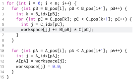
The kernel is further complicated when the result matrix $A$ is sparse, because the assignment to $A$ (line 6) is nested inside the reduction loop $k$. This causes the inner loop $j$ to iterate over and insert into each row of $A$ several times. Sparse data structures, however, do not support fast random inserts (only appends). Inserting into the middle of a CSR matrix costs $\Theta{}(\textrm{nnz})$ because the new value must be inserted into the middle of an array. To get the $\Theta{}(1)$ insertion cost of dense formats, the kernel in Figure 1 introduces a dense workspace. Such workspaces and the accompanying loop transformations are the subject of this paper.

A workspace is a temporary tensor that is typically dense, with fast insertion and random access. Because values can be scattered efficiently into a dense workspace, the loop nest $k,j$ (lines 2–8) in Figure 1 looks similar to the kernel in Figure 1. Instead of assigning values to the result matrix $A$, however, it assigns them to a dense workspace vector. When a row of the result is fully computed in the workspace, it is appended to $A$ in a second loop over $j$ (lines 10–14). This loop iterates over the row in $A$’s sparse index structure, and thus assumes $A$’s CSR index has been pre-assembled. Pre-assembling index structures increases performance when assembly can be moved out of inner loops and is common in material simulations. Section 5 describes the code to assemble result indices by tracking the nonzero coordinates inserted into the workspace.

3. Concrete Index Notation

Specialized compilers for tensor and array operations succeed when they appropriately simplify the space of operations they intend to compile. For this reason, many code generators and computational frameworks for tensor algebra have adopted index notation as the input language to optimize (Kjolstad et al., 2017; Vasilache et al., 2018; Solomonik et al., 2014). Because index notation describes what tensor algebra does but not how it is done, the user does not mix optimization decisions with the algorithmic description. It is therefore easier to separately reason about different implementations, and the algorithmic optimizations described in this work may be applied easily. These advantages come at the cost of restricting the space of operations that can be described.

While index notation is good for describing the desired functionality, it is unsuitable as an intermediate representation within a compiler because it does not encode how the operation should be executed. There are several existing representations one can use to fully describe how an index expression might be computed, such as the code that implements the index expression, sparse extensions of the polyhedral model (Strout et al., 2012; Belaoucha et al., 2010), or iteration graphs (Kjolstad et al., 2017). These representations, however, are so general that it is difficult to determine when it is valid to apply some of the optimizations described in this paper.

We propose a new intermediate language for tensor operations called concrete index notation. Concrete index notation extends index notation with constructs that describe the way that an expression is computed. In the compiler software stack, concrete index notation is an intermediate representation between index notation and the iteration graphs of Kjolstad et al. (2017). A benefit of this design is that we can reason about the legality of optimizations on the concrete index notation without considering sparsity, which is handled by iteration graphs lower in the stack. We generate an expression in concrete index notation as the first step in compiling a tensor expression in index notation provided by the user.

Concrete index notation has three main statement types. The assignment statement assigns an expression result to a tensor element, the forall statement executes a statement over a range inferred from tensor dimensions, and the where statement creates temporaries that store subexpressions.

To give an example, let $A$, $B$, and $C$ be sparse matrices of dimension $I\times J$, $I\times K$, and $K\times J$ where $A$ and $B$ are row-major (CSR) and $C$ is column-major (CSC), and let $t$ be a scalar. Consider the concrete index expression for an inner products matrix multiply, where each element of $A$ is computed with a dot product of a corresponding row of $B$ and column of $C$ (pseudo-code on right):

$\forall_{ijk}\;A_{ij}\mathrel{+}=B_{ik}C_{kj}$

⬇

for $i\in I$

for $j\in J$

for $k\in K$

$A_{ij}\mathrel{+}=B_{ik}*C_{kj}$

The forall statements $\forall_{i}\forall_{j}\forall_{k}$, abbreviated as $\forall_{ijk}$, specify the iteration order of the variables. The resulting loop nest computes in the inner $k$ loop the inner product of the $i$th row of $B$ and the $j$th column of $C$. The statement can be optimized by introducing a scalar temporary $t$ to store the inner products as they are computed. This optimization can improve performance as it is cheaper to accumulate into a scalar due to fewer address calculations. The resulting concrete index notation adds a $\operatorname{\textbf{where}}$ statement that introduces $t$ to hold intermediate computation of each dot product:

$\forall_{ij}\;\left(A_{ij}\operatorname{=}t\right)\operatorname{\textbf{where}}\left(\forall_{k}\;t\mathrel{+}=B_{ik}C_{kj}\right)$

⬇

for $i\in I$

for $j\in J$

$t=0$

for $k\in K$

$t\mathrel{+}=B_{ik}*C_{kj}$

$A_{ij}\operatorname{=}t$

The linear combinations of rows matrix multiply computes rows of $A$ as sums of the rows of $C$ scaled by rows of $B$. When the matrices are sparse, the linear combinations of rows matrix multiply is preferable to inner products matrix multiply for two reasons. First, sparse linear combinations of rows are asymptotically faster because inner products must simultaneously iterate over row/column pairs, which requires iterating over values that are nonzero in only one matrix (Gustavson, 1978). Second, linear combinations of rows work on row-major matrices (CSR), while inner products require the second matrix to be column-major (CSC). It is often more convenient, as a practical matter, to keep matrices ordered the same way. We can express the linear combinations of rows matrix multiply in concrete index notation by moving the $k$ loop above the $j$ loop:

$\forall_{ikj}\;A_{ij}\mathrel{+}=B_{ik}C_{kj}$

⬇

for $i\in I$

for $k\in K$

for $j\in J$

$A_{ij}\mathrel{+}=B_{ik}*C_{kj}$

This algorithm repeatedly computes and adds scaled rows to the matrix $A$. If $A$ is sparse, however, it is very expensive to repeatedly add rows. We therefore add a $\operatorname{\textbf{where}}$ statement that introduces a temporary vector $w$ to hold the partial sums of rows:

$\forall_{i}\;\left(\forall_{j}\;A_{ij}\operatorname{=}w_{j}\right)\operatorname{\textbf{where}}\left(\forall_{kj}\;w_{j}\mathrel{+}=B_{ik}C_{kj}\right)$

⬇

for $i\in I$

$w\operatorname{=}0$

for $k\in K$

for $j\in J$

$w_{j}\mathrel{+}=B_{ik}*C_{kj}$

for $j\in J$

$A_{ij}\operatorname{=}w_{j}$

Note that the temporary $w$ is a vector, while the inner products temporary $t$ was a scalar. The reason is that the we have added the loop $j$ underneath the loop $k$ that we are reducing over. The $j$ loop increases the distance between the production of values on the right-hand-side of the $\operatorname{\textbf{where}}$ and their consumption on the left hand side, and we must therefore increase the dimensionality of the temporary by one to a vector of size equal to the range of $j$.

3.1. Definitions

$$\begin{array}[]{rll}\text{statement}:=&\text{assignment}\\ &\text{forall}\\ &\text{where}\\ &\text{sequence}\\ \text{assignment}:=&\text{access}\,\operatorname{=}\,\text{expr}\\ &\text{access}\,\mathrel{+}=\,\text{expr}\\ &\dots\\ \text{forall}:=&\forall_{\text{index}}\;\;\text{statement}\\ \text{where}:=&\text{statement}\;\operatorname{\textbf{where}}\;\text{statement}\\ \text{sequence}:=&(\text{statement}\operatorname{;\;}\text{statement})*\\ \end{array}$$

$$\begin{array}[]{rll}\text{access}:=&\text{tensor}{}_{\text{indices}}\\ \text{indices}:=&\text{index}{}*\\ \text{expr}:=&\text{literal}\\ &\text{access}\\ &\mathbf{(}\text{expr}{)}\\ &\text{expr}+\text{expr}\\ &\text{expr}\,\text{expr}\hskip 28.45274pt{\color[rgb]{.5,.5,.5}\definecolor[named]{pgfstrokecolor}{rgb}{.5,.5,.5}\pgfsys@color@gray@stroke{.5}\pgfsys@color@gray@fill{.5}//\,multiplication}\\ &\dots\\ \end{array}$$

Figure 2. The grammar of concrete index notation. The construct $\forall_{i\dots k}$ can be used as shorthand for $\forall_{i}\dots\forall_{k}$.

Figure 2 shows the grammar for concrete index notation. Concrete index notation uses index variables to describe the iteration in tensor algebra kernels. Index variables are bound to integer values during execution, and represent tensor coordinates in access expressions. For an order $R$ tensor $A$ and distinct index variables $i_{1},\dots,i_{R}$, the access expression $A_{i_{1}\dots i_{R}}$ represents the single component of $A$ located at coordinate $(i_{1},...,i_{R})$. We sometimes abbreviate an access expression $A_{i_{1}\dots i_{R}}$ as $A_{i\dots}$, and the sequence of index variables is empty when we access a scalar tensor. A scalar expression is defined to be either a literal scalar, an access expression, or the result of applying a binary operator to two scalar expressions, such as $A_{ij}\otimes 2$. Note that binary operators are closed and are pure functions of their inputs.

Scalar expressions represent values, but statements modify the state of programs. We refer to the state of a program in which a statement executes as the environment, consisting of the names of tensors and index variables and the values they hold. To retain some of the intuitive properties of index notation, we restrict statements so that each modifies exactly one tensor.

The first concrete index notation statement we examine is the assignment statement, which modifies the value of a single tensor element. Let $A_{i\dots}$ be an access expression and let $E$ be a scalar expression of variables in the unmodified environment. The assignment statement $A_{i\dots}\operatorname{=}E$ assigns the value represented by $E$ to the element $A_{i\dots}$. Although $E$ cannot contain the tensor $A$, assignment statements may use an optional incrementing form. For some binary operator $\oplus$, executing $(A_{i\dots}\mathrel{\oplus}=E)$ assigns the value $(A_{i\dots}\oplus E)$ to $A_{i\dots}$.

The forall statement repeatedly binds an index variable to an integer value. Let $S$ be a statement modifying the tensor $A$. We require that a particular index variable $i$ in is only used to access modes with matching dimension $D$, so if $i$ appears in $S$, then executing the forall statement $\forall_{i}\;S$ executes $S$ once for each value of $i$ from $D$. Executing $\forall_{i}S$ in the environment $V$ executes $S$ in a copy of $V$ where a new binding $i$ has been added in a local scope, so changes to tensor $A\in V$ are reflected in the original environment but the new binding for $i$ is not. To avoid overwriting tensor values, we add a new constraint. If $\forall_{i}S$ is a statement that modifies a tensor $A$ in an assignment statement $A_{j\dots}\operatorname{=}E$, then $i$ must be one of the index variables $j\dots$ which has not yet been bound by $S$. We introduce multiple forall syntax to simplify writing multiple nested foralls in a row. Thus, $\forall_{i\dots}\;S$ is equivalent to $\forall_{i_{1}}\;\forall_{i_{2}}\;...S$.

The where statement precomputes a tensor subexpression. Let $S$ and $S^{\prime}$ be statements which modify tensors $A$ and $A^{\prime}$ respectively. The where statement $(S\,\operatorname{\textbf{where}}\,S^{\prime})$ then modifies the tensor $A$. We execute the where statement $(S\,\operatorname{\textbf{where}}\,S^{\prime})$ in an environment $V$ in two steps. First, we execute $S^{\prime}$ in a copy of $V$ where $A$ has been removed. Since our statement may only modify $A$, $A^{\prime}$ must not already be a variable in $V$ or this expression would modify multiple tensors (we discuss the special case where $A^{\prime}$ and $A$ are the same tensor in the next paragraph). Next, we execute $S$ in a copy of $V$ where $A^{\prime}$ has been added. Note that this second step does not add $A^{\prime}$ to $V$, but changes to $A$ in this new environment are reflected in $V$.

The sequence statement modifies the same tensor multiple times in sequence. The sequence statement $(S^{\prime};\,S)$ is like a where statement, except the order of $S$ and $S^{\prime}$ is swapped and instead of restricting $A^{\prime}$ to be a variable not in $V$, we say that $A^{\prime}$ must be equal to $A$. Thus, the same tensor is modified multiple times in a sequence. We may simplify multiple nested sequence expressions in a row by omitting parenthesis so that $(S_{0}\operatorname{;\;}S_{1}\operatorname{;\;}S_{2}\operatorname{;\;}\dots)$ is equivalent to $((S_{0}\operatorname{;\;}S_{1})\operatorname{;\;}S_{2})\operatorname{;\;}\dots)$.

Finally, we describe when to initialize tensors. Notice that the only two terminal statements in concrete index notation are the assignment statement and the increment statement. Recall that each statement modifies exactly one tensor. Before executing a concrete index statement that modifies a tensor $A$ with an increment statement $A_{i\dots}\mathrel{\oplus}=E$, if $A$ is not defined in the environment then $A$ is initialized to the identity element for the binary operation $\oplus$.

3.2. Relationship to Index Notation

Index notation is a compact notation for tensor operations that does not specify how they are computed. If $E$ is a scalar expression, the index expression $A_{i\dots}=E$ evaluates $E$ for each value of $i\dots$ in the dimensions of $A$ and sets $A_{i\dots}$ equal to the result. In this work, we disallow the tensor $A$ from appearing in $E$. We introduce a scalar expression for index notation called the reduction expression. The reduction expression $\sum_{i\dots}E$ over the scalar expression $E$ evaluates to the sum of $E$ evaluated over the distinct values $i\dots$.

As an example, the following expression in index notation computes matrix multiplication:

$$A_{ij}=\sum_{k}B_{ik}C_{kj}$$

We can trivially convert an expression $A_{i\dots}=E_{I}$ in index notation to a statement in concrete index notation $S_{C}$ as follows:

Let $S_{C}$ be $A_{i\dots}=E_{I}$

while $S_{C}$ contains reduction nodes do

     Let $R=\sum_{j\dots}E_{I}$ be a reduction node in $S_{C}$.

     Replace $R$ with a fresh variable $t$ in $S_{C}^{\prime}$

     Replace $S_{C}^{\prime}$ with $S_{C}^{\prime}\operatorname{\textbf{where}}(\forall_{j\dots}\;t\mathrel{+}=E_{I})$

end while

Return $\forall_{i\dots}\;S_{C}$

The algorithm is improved if $R$ is always one of the outermost reduction nodes in one of the the leftmost assignment statements $S_{C}^{\prime}$ within $S_{C}$ that contains a reduction expression.

3.3. Reordering

Reordering concrete index notation statements is useful for several reasons. First, sparse tensors are sensitive to the order in which they are accessed. For example, iterating over rows of a CSC matrix is costly. We can reorder forall statements to yield better access patterns. We may also wish to reorder to move loop-invariant where statements out of inner loops. Critically, we may need to reorder statements so that the preconditions for our workspace optimization apply. When we reorder a concrete index statement, we want to know that it will do the same thing as it used to. We can express this semantic equivalence by breaking down the transformation into small pieces.

We start by showing when we can rearrange forall statements. Let $S$, $\forall_{i}\;\forall_{j}\;S$, and $\forall_{j}\;\forall_{i}\;S$ be valid statements in concrete index notation which do not contain sequence statements. If $S$ modifies its tensor with an assignment statement or an increment statement with an associative operator, then $\forall_{i}\;\forall_{j}\;S$ and $\forall_{j}\;\forall_{i}\;S$ are semantically equivalent.

Next, we show when we can move a forall out of the left hand side of a where statement. Let $S_{1}$, $S_{2}$, $(\forall_{j}\;S_{1})\operatorname{\textbf{where}}S_{2}$, and $\forall_{j}\;(S_{1}\operatorname{\textbf{where}}S_{2})$ be concrete index statements which do not contain sequence statements. If $S_{2}$ does not use the index variable $j$, then $(\forall_{j}\;S_{1})\operatorname{\textbf{where}}S_{2}$ and $\forall_{j}\;(S_{1}\operatorname{\textbf{where}}S_{2})$ are semantically equivalent.

We can also move a forall out of both sides of a where statement. Let $S_{1}$, $S_{2}$, $(\forall_{j}\;S_{1})\operatorname{\textbf{where}}(\forall_{j}\;S_{2})$, and $\forall_{j}\;(S_{1}\operatorname{\textbf{where}}S_{2})$ be concrete index statements which do not contain sequence statements. If $S_{2}$ modifies its tensor with an assignment statement, then $(\forall_{j}\;S_{1})\operatorname{\textbf{where}}(\forall_{j}\;S_{2})$ and $\forall_{j}\;(S_{1}\operatorname{\textbf{where}}S_{2})$ are semantically equivalent.

Of course, we must rearrange nested where statements. We start by reordering nests. Let $S_{1}$, $S_{2}$, $S_{3}$, $(S_{1}\operatorname{\textbf{where}}S_{2})\operatorname{\textbf{where}}S_{3}$, and $S_{1}\operatorname{\textbf{where}}(S_{2}\operatorname{\textbf{where}}S_{3})$ be concrete index statements which do not contain sequence statements. If $S_{1}$ does not use the tensor modified by $S_{3}$, then $(S_{1}\operatorname{\textbf{where}}S_{2})\operatorname{\textbf{where}}S_{3}$, and $S_{1}\operatorname{\textbf{where}}(S_{2}\operatorname{\textbf{where}}S_{3})$ are semantically equivalent.

We can also reorder right hand sides of $\operatorname{\textbf{where}}$ statements. Let $S_{1}$, $S_{2}$, $S_{3}$, $(S_{1}\operatorname{\textbf{where}}S_{2})\operatorname{\textbf{where}}S_{3}$, and $(S_{1}\operatorname{\textbf{where}}S_{3})\operatorname{\textbf{where}}S_{2}$ be concrete index statements which do not contain sequence statements. If $S_{2}$ does not use the tensor modified by $S_{3}$ and $S_{3}$ does not use the tensor modified by $S_{2}$, then $(S_{1}\operatorname{\textbf{where}}S_{2})\operatorname{\textbf{where}}S_{3}$, and $(S_{1}\operatorname{\textbf{where}}S_{3})\operatorname{\textbf{where}}S_{2}$ are semantically equivalent.

4. Workspace Optimization

The workspace optimization extracts and pre-computes tensor algebra sub-expressions into a temporary workspace, using the concrete index notation’s $\operatorname{\textbf{where}}$ statement. The workspace optimization can optimize sparse tensor algebra kernels in the following three ways:

Simplify merges:

Code to simultaneously iterate over multiple sparse tensors contains conditionals and loops that may be expensive. By computing sub-expressions in dense workspaces, the code instead iterates over a sparse and dense operands (e.g., Figure 3).

Avoid expensive inserts:

Inserts into the middle of a sparse tensor, such as an increment inside of a loop, are expensive. We can improve performance by computing the results in a workspace that supports fast inserts, such as a dense array or a hash map (e.g., Figure 8).

Hoist loop invariant computations:

Computing a whole expression in the inner loop sometimes results in redundant computations. Pre-computing a sub-expression in a separate loop and storing it in a workspace can hoist parts of a loop out of a parent loop (e.g., Figure 10).

Many important sparse tensor algebra kernels benefit from the workspace optimization, including sparse matrix multiplication, matrix addition, and the matricized tensor times Khatri-Rao product. In this section we describe the optimization and give simple examples, and we will explore its application to sophisticated real-world kernels in Section 6.

To separate mechanism (how to apply it) and policy (whether to apply it), the workspace optimization is programatically asked for using the workspace method. The method applies to an expression on the right-hand-side of an index notation statement, and takes as arguments the index variables to apply the workspace optimization to and a format that specifies whether the workspace should be dense or sparse. Implemented in C++, the API is

⬇

void IndexExpr::workspace(std::vector<IndexVar> variables, Format format);

It can be used to generate the code in Figure 1 as follows:

⬇

1Format CSR({dense, sparse});

2TensorVar A(CSR), B(CSR), C(CSR);

3IndexVar i, k, j;

4

5IndexExpr mul = B(i,k) * C(k,j);

6A(i,j) = sum(k)(mul);

7

8mul.workspace({j}, Format(dense));

Lines 1–3 creates a CSR format, three tensor variables, and three index variables to be used in the computation. Lines 5–6 defines a sparse matrix multiplication with index notation. Finally, line 8 declares that the multiplication should be pre-computed in a workspace, by splitting the j loop into two j loops. The optimization performs the following transformation on the concrete index notation produced from the index notation:

$$\forall_{ikj}\;A_{ij}\mathrel{+}=B_{ik}C_{kj}\implies\forall_{i}\;\left(\forall_{j}\;A_{ij}\operatorname{=}w_{j}\right)\operatorname{\textbf{where}}\left(\forall_{kj}\;w_{j}\mathrel{+}=B_{ik}C_{kj}\right),$$

and result in the code shown on lines 2–9 in Figure 1.

$\forall_{ij}\;a_{i}\mathrel{+}=B_{ij}C_{ij}$

(a) Before optimization the kernel iterates over the sparse intersection of each row of $B$ and $C$, by simultaneously iterating over their index structures to check if both have coordinates at each point.

$\forall_{i}\;\left(\forall_{j}\;a_{i}\mathrel{+}=w_{j}C_{ij}\right)\operatorname{\textbf{where}}\left(\forall_{j}\;w_{j}\operatorname{=}B_{ij}\right)$

(b) The workspace optimization introduces a $\operatorname{\textbf{where}}$ statement that results in two loops. The first copies $B$ to a dense workspace $w$, and the second computes $A$ by iterating over $C$ and randomly accessing $w$.

Figure 3. Kernels that compute the sparse inner product of each pair of rows in the CSR matrices $B$ and $C$ $a_{i}=\sum_{j}B_{ij}C_{ij}$ before and after applying the workspace optimization to the matrix $B$ over $j$. Sparse code generation is addressed in Section 5.

4.1. Definition and Preconditions

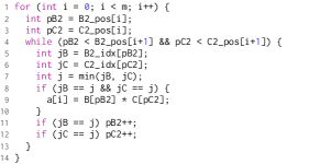
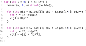
The workspace optimization rewrites concrete index notation to pre-compute a sub-expression. The effect is that an assignment statement is split in two, where one statement produces values for the other through a workspace. Figure 3 shows concrete index notation and kernels that compute the inner product of each pair of rows from two matrices, before and after the workspace optimization is applied to the matrix $B$ over $j$. In this example the optimization causes the while loop over $j$, that simultaneously iterates over the two rows, to be replaced with a for loop that independently iterates over each of the rows. The for loops have fewer conditionals, at the cost of reduced data locality. Note that sparse code generation is handled below the concrete index notation in the compiler stack, as described in Section 5.

Let $(S,E,i\dots)$ be the inputs to the optimization, where $S$ is a statement not containing sequences, $i\dots$ is a set of index variables, and $E$ is an expression contained in an assignment or increment statement $S_{A}$ contained in $S$. If $S_{A}$ is the increment statement, let $\oplus$ be the associated operator. The optimization rewrites the statement $S_{A}$ to precompute $E$ in a workspace. This operation may only be applied if every operator on the right hand side of $S_{A}$ which contains $E$ distributes over $\oplus$.

Let $S_{A}^{\prime}$ be $S_{A}$ where $E$ has been replaced by the access expression $w_{i\dots}$ where $w$ is a fresh tensor variable.

In $S$, replace $S_{A}$ with $S_{A}^{\prime}\operatorname{\textbf{where}}(w_{i\dots}\mathrel{\oplus}=E)$.

Let $S_{w}$ be this where statement.

while $S_{w}$ is contained in a forall statement over an index variable $j$ do

     if $j$ is used in both sides of $S_{w}$ and $j\in i\dots$ then

         Move $\forall_{j}$ into both sides of $S_{w}$.

     else if $j$ is used only in the left side of $S_{w}$ then

         Move $\forall_{j}$ into the left side of $S_{w}$.

     else if $j$ is used only in the right side of $S_{w}$ then

         Move $\forall_{j}$ into the right side of $S_{w}$.

     else

         Stop.

     end if

end while

The arrangement of the forall statements containing $S$ affects the results of the optimization, so we may want to reorder before it is applied. The order (dimensionality) of the resulting workspace is the number of index variables in $i\dots$ and the dimension sizes are equal to the ranges of those index variables in the existing expression.

4.2. Result Reuse

When applying a workspace optimization $(S,E,i\dots)$ it sometimes pays to use the left hand side of the assignment statement $S_{A}$ that contains $E$ as a workspace. Thus the expression $E$ is assigned to $w$ followed by $S_{A}$ rewritten as a incrementing assignment. To support such mutation, we use the sequence statement, which allows us to define a result and compute it in stages. Result reuse is for example useful when applying the workspace optimization to sparse vector addition with a dense result, as the partial results can be efficiently accumulated into the result,

$$\forall_{i}\;a_{i}\operatorname{=}b_{i}+c_{i}\implies\left(\forall_{i}\;a_{i}\operatorname{=}b_{i}\operatorname{;\;}\forall_{i}\;a_{i}\mathrel{+}=c_{i}\right).$$

The workspace optimization can reuse the result as a workspace if two preconditions are satisfied. The first precondition requires that the forall statements on the two sides of the $\operatorname{\textbf{where}}$ statement are the same. That is, that the optimization does not hoist any computations out of a loop. This precondition ensures that the result does not get over-written by its use as a workspace and is, for example, not satisfied by the second workspace optimization to the MTTKRP kernel in Section 6.3. The second precondition is that the expression $E$ is nested inside at most one operator in $S_{E}$, which ensures we can rewrite the top expression to an incrementing assignment.

$\forall_{ij}\;A_{ij}\operatorname{=}B_{ij}+C_{ij}$

(a) Before optimization the kernel iterates over the sparse union of each row of $B$ and $C$, by simultaneously iterating over their index structures to check if either have a coordinate at each point.

$\forall_{i}\;\left(\forall_{j}\;A_{ij}\operatorname{=}w_{j}\right)\operatorname{\textbf{where}}\left(\forall_{j}\;w_{j}\operatorname{=}B_{ij}\operatorname{;\;}\forall_{j}\;w_{j}\mathrel{+}=C_{ij}\right)$

(b) The workspace optimizations introduces a $\operatorname{\textbf{where}}$ statement with a sequence that results in three loops. The first two adds $B$ and $C$ to $w$ and the second stores the results to $A$.

Figure 4. Sparse matrix addition $A_{ij}=B_{ij}+C_{ij}$ with CSR matrices before and after applying the workspace optimization twice over $j$. The first application is to the $B_{ij}+C_{ij}$ expression, while the second application is to $B$ and reuses the workspace $w$ resulting in a sequence statement and the kernel above.

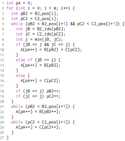
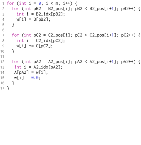
Figure 4 shows a sparse matrix addition with CSR matrices before and after applying the workspace optimization twice, resulting in a kernel with three loops. The first two loops add each of the operands $B$ and $C$ to the workspace, and the third loop copies the non-zeros from the workspace to the result $A$. The first workspace optimization applies to the sub-expression $B_{ij}+C_{ij}$ over $j$ resulting in

$$\forall_{i}\;\left(\forall_{j}\;A_{ij}\operatorname{=}w_{j}\right)\operatorname{\textbf{where}}\left(\forall_{j}\;w_{j}\operatorname{=}B_{ij}+C_{ij}\right).$$

The second transformation applies to the $B_{ij}$ sub-expression on the right-hand side of the $\operatorname{\textbf{where}}$. Without result reuse the result would be

$$\forall_{i}\;\left(\forall_{j}\;A_{ij}\operatorname{=}w_{j}\right)\operatorname{\textbf{where}}\left(\left(\forall_{j}\;w_{j}\operatorname{=}v_{j}+C_{ij}\right)\operatorname{\textbf{where}}\left(\forall_{j}\;v_{j}\operatorname{=}B_{ij}\right)\right),$$

but with result reuse the two operands are added to the same workspace in a sequence statement

$$\forall_{i}\;\left(\forall_{j}\;A_{ij}\operatorname{=}w_{j}\right)\operatorname{\textbf{where}}\left(\forall_{j}\;w_{j}\operatorname{=}B_{ij}\operatorname{;\;}\forall_{j}\;w_{j}\mathrel{+}=C_{ij}\right).$$

4.3. Policy and Choice of Workspace

The workspace optimization increases the performance of many important kernels by removing inserts into sparse results, expensive merge code, and loop invariant code. It does, however, impose costs from constructing, maintaining, and using workspaces. Constructing a workspace requires a malloc followed by a memset to zero its values and it must be reinitialized between uses. Furthermore, a workspace reduces temporal locality due to the increased reuse distance from storing values to the workspace and later reading them back to store to the result.

System designs are more flexible when they separate mechanism (what to do) from policy (how to do it) (Hansen, 1970; Wulf et al., 1974). Performance is a key design criteria in tensor algebra systems, so they should separate the policy decisions of how to optimize code from the mechanisms that carry out the optimization. This paper focuses on optimization mechanisms.

We envision many fruitful policy approaches such as user-specified policy, heuristics, mathematical optimization, machine learning, and autotuning. We leave the design of automated policy systems as future work. To facilitate policy research, however, we have described an API for specifying workspace optimizations. We see this API as part of a scheduling language for index notation. The Halide system (Ragan-Kelley et al., 2012) has shown that a scheduling language is effective at separating optimization mechanism from policy. Scheduling languages leave users in control of performance, while freeing them from low level code transformations. The goal, of course, is a fully automated system where users are freed from performance decisions as well. Such a system, however, also profits from a well-designed scheduling language, because it it lets researchers explore different policy approaches without re-implementing mechanisms.

Furthermore, dense arrays are not the only choice for workspaces; a tensor of any format will do. The format, however, affects the generated code and its performance. The workspace optimization can be used to remove expensive sparse-sparse merge code, and dense workspaces are attractive because they result in cheaper sparse-dense merges. An alternative is another format with random access such as a hash map. These result in slower execution (Patwary et al., 2015), but only use memory proportional to the number of nonzeros.

5. Compilation

Concrete index notation is an effective intermediate representation for describing important optimizations on index notation such as the workspace optimization. In this section we show how concrete index notation on sparse and dense tensors is compiled to code. We build on the work of Kjolstad et al., which details a compiler for sparse tensor expressions represented with an intermediate representation called iteration graphs (2017). We describe a process to convert concrete index notation to iteration graphs that can then be compiled with their system. We also show how their code generation machinery can be extended to assemble workspace indices.

The iteration graph intermediate representation for tensor algebra compilation describes the constraints imposed by sparse tensors on the iteration space of index variables (Kjolstad et al., 2017). Sparse tensors provide an opportunity and a challenge. They store only nonzeros and loops therefore avoid iterating over zeros, but they also enforce a particular iteration order because they encode tensor coordinates hierarchically.

We construct iteration graph from concrete index notation, such as $\forall_{iklj}\;A_{ij}\mathrel{+}=B_{ilk}C_{lj}D_{kj}$ or $\forall_{ij}\;a_{i}\mathrel{+}=B_{ij}c_{j}+d_{i}$. In concrete index notation, index variables range over the dimensions they index and computations occur at each point in the iteration space. Index variables are nodes in iteration graphs and each tensor access, such as $B_{ij}$, becomes a path through the index variables.

(a) $A_{ij}=\sum_{k}B_{ik}C_{kj}$

(b) $A_{ijk}=B_{ijk}+C_{ijk}$

(c) $A_{ij}=\sum_{k}B_{ij}C_{ik}D_{kj}$

(d) $A_{ij}=\sum_{lk}B_{ikl}C_{lj}D_{kj}$

Figure 5. Four iteration graphs: (5) matrix multiplication, (5) tensor addition, (5) sampled dense-dense matrix multiplication (SDDMM), and (5) matricized tensor times Khatri-Rao product (MTTKRP).

Figure 5 shows several iteration graphs, including matrix multiplication, sampled dense-dense matrix multiplication from machine learning (Zhao, 2014), and the matricized tensor times Khatri-Rao product used to factorize tensors (Bader and Kolda, 2007). The concrete index notation for tensor-vector multiplication is, for example,

$$\forall_{ijk}\;A_{ij}\mathrel{+}=B_{ijk}c_{k}.$$

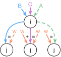
The corresponding iteration graph in Figure 6 has a node for each index variable $i$, $j$, and $k$ and a a path for each of the three tensor accesses $B_{ijk}$ (blue), $c_{k}$ (purple), and $A_{ij}$ (stippled green). We draw stippled paths for results. Figure 6 shows code generated from this iteration graph when $B$ and $c$ are sparse. Each index variable node becomes a loop that iterates over the sparse tensor indices belonging to the incoming edges.

(a) Iteration Graph

(b) Generated code when $A$ is dense while $B$ and $c$ are sparse.

Figure 6. Tensor-vector multiplication $A_{ij}=\sum_{k}B_{ijk}c_{k}$. Each index variable becomes a loop over the sparse tensor indices of its incoming paths. The $k$ loop iterates over the intersection of the last dimension of $B$ and $c$.

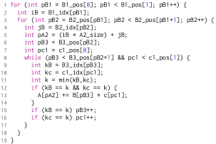
Two or more input paths meet at an index variable when it is used to index into two or more tensors. The iteration space of the tensor dimensions the variable indexes must be merged in the generated code. The index variables are annotated with operators that tell the code generator what kind of merge code to generate. If the tensors are multiplied then the generated code iterates over the intersection of the indexed tensor dimensions (Figure 3). If they are added then it iterates over their union (Figure 4). If more than two tensors are indexed by the same index variable, then code is generated to iterate over a mix of intersections and unions of tensor dimensions.

Iteration graphs are a hierarchy of index variable nodes, together with tensor paths that describe tensor accesses. Constructing an iteration graph from concrete index notation is a two-step process:

Construct Index Variable Hierarchy:

To construct the index variable hierarchy, traverse the concrete index notation. If the forall statement of an index variable $j$ is nested inside the forall statement of index variable $i$, then we also place $j$ under $i$ in the iteration graph. Furthermore, the index variables of two forall statements on different sides of a $\operatorname{\textbf{where}}$ statement become siblings.

Add Tensor Paths:

To add the paths, visit each tensor access expression. For each access expression, add a path between the index variables used to access the tensor. The order of the path is determined from the order the dimensions are stored. If, for example, the access expression is $B_{ij}$ then add the path $(i,j)$ if the matrix is row major (e.g., CSR) and the path $(j,i)$ if the matrix is column major (e.g., CSC).

Kjolstad et al. described an algorithm to generate code from iteration graphs, including a mechanism called merge lattices to generate code to co-iterate over tensor dimensions (2017). Understanding our workspace optimization does not require understanding the details of the code generation algorithm or merge lattices. We should note, however, that the performance of code that merges sparse tensors may suffer from many conditionals. Code to co-iterate over a combination of a single sparse and one or more dense tensors, on the other hand, does not require conditionals. One of the benefits of introducing a workspace is to improve performance by turning sparse-sparse iteration into sparse-dense iteration.

Figure 7. Sparse matrix multiply assembly kernel (the compute kernel is in Figure 1). The coordinates of row $i$ are inserted into wlist on line 11 and copied to A on line 28. The array w guards against redundant inserts.

In code listings that compute sparse results, we have so far shown only kernels that compute results without assembling sparse index structures (Figures 1, 4, and 10). This let us focus on the loop structures without the added complexity of workspace assembly. Moreover, it is common in numerical code to separate the kernel that assembles index structures (often called symbolic computation) from the kernel that computes values (numeric computation) (Gustavson, 1978; Heath et al., 1991). The code generation algorithm for iteration graphs can emit either, or a kernel that simultaneously assembles the result index structures and computes its values.

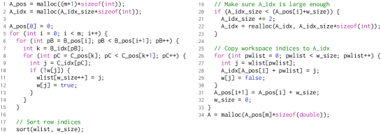
When generating assembly kernels from iteration graphs, a workspace consists of two arrays that together track its nonzero index structure. The first array wlist is a list of coordinates that have been inserted into the workspace, and the second array (w) is a boolean array that guards against redundant inserts into the coordinate list.

Figure 7 shows assembly code for sparse matrix multiplication generated from the iteration graph in Figure 8. It is generated from the same iteration graph as the compute kernel in Figure 1, so the loop structure is the same except for the loop to copy the workspace to A on line 26. In compute kernels, the index structure of A must be pre-assembled, so the code generation algorithm emits a loop to iterate over A. In an assembly kernel, however, it emits code to iterate over the index structure of the workspace. Furthermore, the assembly kernel inserts into the workspace index (wlist), on lines 10–13, instead of computing a result, and sorts the index list on line 18 so that the new row of A is ordered. Note that the sort is optional and only needed if the result must be ordered. Finally, the assembly kernel allocates memory on lines 1–2, 20–23 (by repeated doubling), and 34.

6. Case Studies

In this section we study three important linear and tensor algebra expressions that can be optimized with the workspace optimization. The resulting kernels are competitive with hand-optimized kernels from the literature (Gustavson, 1978; Smith et al., 2015; Guennebaud et al., 2010). The optimization, however, generalizes to an uncountable number of kernels that have not been implemented before. We will show one example, MTTKRP with sparse matrices, in Section 6.3.

6.1. Matrix Multiplication

$\forall_{ikj}\;A_{ij}\mathrel{+}=B_{ik}C_{kj}$

(a) Iteration graph before workspace optimization

$\forall_{i}\;(\forall_{j}\;A_{ij}\operatorname{=}w_{j})\,\operatorname{\textbf{where}}\;(\forall_{kj}\;w_{j}\mathrel{+}=B_{ik}C_{kj})$

(b) Iteration graph after workspace optimization

Figure 8. Matrix multiplication $A_{ij}=\sum_{k}B_{ik}C_{kj}$ using the linear combination of rows algorithm with all matrices in the CSR format. Pre-computing row-computations in a workspace recreates Gustavson’s algorithm (1978) shown showed Figure 1.

The preferred algorithm for multiplying two sparse matrices is to compute the linear combinations of rows or columns (Guennebaud et al., 2010; Davis, 2006; MATLAB, 2014; Bezanson et al., 2012). This algorithm was introduced by Gustavson (1978), who showed that it is asymptotically superior to computing inner products when the matrices are sparse. Furthermore, both operands and the result are the same format. A sparse inner product algorithm inconveniently needs the first operand to be row major (CSR) and the second column major (CSC).

Figure 8 shows the concrete index notation and iteration graph for a linear combination of rows algorithm, where the matrices are stored in the CSR format. The iteration graph shows an issue at index variable $j$. Because the assignment to $A$ at $j$ is dominated by the summation index variable $k$ in the iteration graph, the generated code must repeatedly add new values into $A$. This is expensive when $A$ is sparse due to costly inserts into its sparse data structure.

In Figure 8, the concrete index notation has been optimized to pre-compute the $B_{ik}C_{kj}$ sub-expression in a workspace. In the resulting iteration graph this results in $j$ being split into two new index variables. The first accumulates values into a dense workspace $w$, while $j_{A}$ copies the nonzero values from the workspace to $A$. Because the workspace is dense, the merge with $C$ at $j_{C}$ is trivial: the kernel iterates over $C$ and scatters values into $w$. Furthermore, the second index variable $j_{A}$ is not dominated by the summation variable $k$ and values are therefore appended to $A$.

The code listing in Figure 1 showed the code generated from a matrix multiplication iteration graph where the assignment operator has been split. Each index variable results in a loop, loops generated from index variables connected by an arrow are nested, and loops generated from index variables that share a direct predecessor are sequenced. The last $j$ loop copies values from the workspace to $A$, so it can either iterate over the nonzeros of the workspace or the index structure of $A$. The loop on lines 10–14 in the code listing iterates over the index structure of $A$, meaning it must be pre-assembled before this code is executed. The alternative is to emit code that tracks the nonzeros inserted into the workspace, but this is more expensive. It is sometimes more efficient to separate the code that assembles $A$’s index structure from the code that computes its values (Gustavson, 1978). We discussed code generation for pure assembly and fused assembly-and-compute kernels in Section 5. These kernels cannot assume the results have been pre-assembled and must maintain and iterate over a workspace index.

6.2. Matrix Addition

Sparse matrix addition demonstrates the workspace optimization for addition operators. Sparse additions result in code to iterate over the union of the nonzeros of the operands, as a multi-way merge with three loops  (Knuth, 1973). Figure 9 shows the concrete index notation and iteration graph for a sparse matrix addition. When the matrices are stored in the CSR format, which is sparse in the second dimension, the compiler must emit code to merge $B$ and $C$ at the $j$ index variable. Such merge code contains many if statements that are expensive on modern processors. Merge code also grows exponentially with the number of additions, so if many matrices are added it is necessary to either split the input expression or, better, to use the workspace optimization at the inner index variable so that the outer loop can still be shared.

$\forall_{ij}\;A_{ij}=B_{ij}+C_{ij}$

(a) Iteration graph workspace optimizations

$\forall_{i}\;(\forall_{j}\;A_{ij}\operatorname{=}w_{j})\,\operatorname{\textbf{where}}\;(\forall_{j}\;w_{j}\operatorname{=}B_{ij}\operatorname{;\;}\forall_{j}\;w_{j}\mathrel{+}=C_{ij})$

(b) Iteration graph after workspace optimizations

Figure 9. Sparse matrix addition $A_{ij}=B_{ij}+C_{ij}$. Splitting the addition and assignment operators removes expensive merge code at the cost of reduced temporal locality. The code before and after the split are shown in in Figure 4.

Applying the workspace optimization twice to both $B$ and $C$ at $j$ introduces a dense row workspace that rows of $B$ and $C$ are in turn are added into, and that is then copied over to $A$. The resulting code was shown in Figure 4 and has decreased temporal locality due to the workspace reuse distance, but avoids expensive merges. Whether this results in an overall performance gain depends on the machine, the number of operands that are merged, and the nonzero structure of the operands. We show results in Figure 14.

6.3. Matricized Tensor Times Khatri-Rao Product

(a) Before workspace optimization

$\forall_{ik}\;\left(\forall_{j}\;A_{ij}\mathrel{+}=w_{j}D_{kj}\right)\operatorname{\textbf{where}}\left(\forall_{lj}\;w_{j}\mathrel{+}=B_{ikl}C_{lj}\right)$

(b) After optimization to pre-compute $B_{ikl}C_{lj}$ in workspace $w$ at $j$. The code diff shows the effect of the transformation.

$\forall_{i}\;\left(\forall_{j}\;A_{ij}\operatorname{=}v_{j}\right)\operatorname{\textbf{where}}\left(\forall_{k}\;\left(\forall_{j}\;v_{j}\mathrel{+}=w_{j}D_{kj}\right)\operatorname{\textbf{where}}\left(\forall_{lj}\;w_{j}\mathrel{+}=B_{ikl}C_{lj}\right)\right)$

(c) After further optimization to pre-compute $w_{j}D_{kj}$ in workspace $v$ at $j$. The code diff shows the effect of the transformation.

Figure 10. The matricized tensor times Khatri-Rao product (MTTKRP) $A_{ij}=\sum_{kl}B_{ikl}C_{lj}D_{kj}$. Workspacing $B_{ikl}C_{lj}$ at $j$ hoists the expression out of the $l$ loop and therefore removes redundant loop-invariant work. If the matrix $A$ is sparse, then also workspacing $w_{j}D_{kj}$ at $j$ introduces a random access workspace that removes the need to insert into $A$.

The matricized tensor times Khatri-Rao product (MTTKRP) is the critical kernel in the alternating least squares algorithm to compute the canonical polyadic decomposition of tensors (Hitchcock, 1927). The canonical polyadic decomposition generalizes the singular value decomposition to higher-order tensors, and has applications in data analytics (Cichocki, 2014), machine learning (Phan and Cichocki, 2010), neuroscience (Möcks, 1988), image classification and compression (Shashua and Levin, 2001), and other fields (Kolda and Bader, 2009).

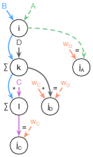
The MTTKRP can be expressed with tensor index notation as $A_{ij}=\sum_{kl}B_{ikl}C_{lj}D_{kj}$. That is, we multiply a three-dimensional tensor by two matrices in the $l$ and $k$ dimensions. These simultaneous multiplications require four nested loops. Figure 10 shows the iteration graph before optimization, where the matrices are stored row-major. The iteration graph results in four nested loops. The three outermost loops iterate over the sparse data structure of $B$, while the innermost loop iterates over the range of the $j$ index variable.

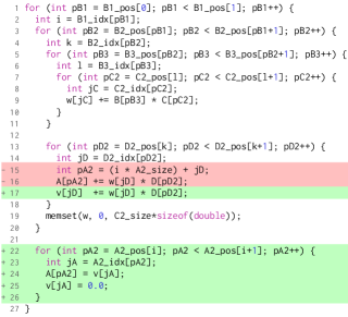
After applying the workspace optimization to the expression $B_{ikl}C_{lj}$ at $j$ we get the iteration graph in Figure 10. The index variable $j$ has been split in two. The second $j$ is no longer dominated by $l$ and is therefore evaluated higher up in the resulting loop nest. Furthermore, if the matrices $C$ and $D$ are sparse in the second dimension, then the workspace optimization also removes the need to merge their sparse data structures. The code listing in Figure 10 shows a code diff of the effect of the optimization on the code when the matrices are dense. The code specific to the iteration graph before optimizing is colored red, and the code specific to the iteration graph after optimizing is colored green. Shared code is not colored. The workspace optimization results in code where the loop over $j$, that multiplies $B$ with $D$, has been lifted out of the $l$ loop, resulting in fewer total multiplication. The drawback is that the workspace reduces temporal locality, as the reuse distance between writing values to it and reading them back can be large. Our evaluation in Figure 12 shows that this optimization can result in significant gains on large data sets.

The MTTKRP kernel does two simultaneous matrix multiplications. Like the sparse matrix multiplication kernel in Section 6.1, it scatters values into the middle of the result matrix $A$. The reason is that the $j$ index variables are dominated by reduction variables. If the matrix $A$ is sparse then inserts are expensive and the code profits from applying the workspace optimization again to pre-compute $w_{j}D_{kj}$ in a workspace, as shown in Figure 10. The effect is that values are scattered into a dense workspace with random access and copied to the result after a full row of the result has been computed. Figure 10 shows a code diff of the effect of making the result matrix $A$ sparse and pre-computing $w_{j}D_{kj}$ in a workspace $v$. Both the code from before optimization (red) and the code after (green) assumes the operand matrices $C$ and $D$ are sparse, as opposed to Figure 10 where $C$ and $D$ were dense. As in the sparse matrix multiplication code, the code after the workspace optimization scatters into a dense workspace $v$ and, when a full row has been computed, appends the workspace nonzeros to the result.

7. Evaluation

In this section, we evaluate the effectiveness of the workspace optimization by comparing the performance of sparse kernels with workspaces against hand-written state-of-the-art sparse libraries for linear and tensor algebra.

Table 1. Test matrices from the SuiteSparse Matrix Collection (Davis and Hu, 2011) and test tensors from the FROSTT Tensor Collection (Smith et al., 2017b).

Tensor	Domain	NNZ	Density
bcsstk17	Structural	428,650	4E-3
pdb1HYS	Protein data base	4,344,765	3E-3
rma10	3D CFD	2,329,092	1E-3
cant	FEM/Cantilever	4,007,383	1E-3
consph	FEM/Spheres	6,010,480	9E-4
cop20k	FEM/Accelerator	2,624,331	2E-4
shipsec1	FEM	3,568,176	2E-4
scircuit	Circuit	958,936	3E-5
mac-econ	Economics	1,273,389	9E-5
pwtk	Wind tunnel	11,524,432	2E-4
webbase-1M	Web connectivity	3,105,536	3E-6
Facebook	Social Media	737,934	1E-7
NELL-2	Machine learning	76,879,419	2E-5
NELL-1	Machine learning	143,599,552	9E-13

7.1. Methodology

All experiments are run on a dual-socket 2.5 GHz Intel Xeon E5-2680v3 machine with 12 cores/24 threads and 30 MB of L3 cache per socket, running Ubuntu 14.04.5 LTS. The machine contains 128 GB of memory and runs Linux kernel version 3.13.0 and GCC 5.4.0. For all experiments, we ensure the machine is otherwise idle and report average cold cache performance, without counting the first run, which often incurs dynamic loading costs and other first-run overheads. The experiments are single-threaded unless otherwise noted.

We evaluate our approach by comparing performance on linear algebra kernels with Eigen (Guennebaud et al., 2010) and Intel MKL (Intel, 2012) 2018.0, and tensor algebra kernels against the high-performance SPLATT library for sparse tensor factorizations (Smith et al., 2015). We obtained real-world matrices and tensors for the experiments in Sections 7.2 and 7.3 from the SuiteSparse Matrix Collection (Davis and Hu, 2011) and the FROSTT Tensor Collection (Smith et al., 2017b) respectively. Details of the matrices and tensors used in the experiments are shown in Table 1. We constructed the synthetic sparse inputs using the random matrix generator in taco, which places nonzeros randomly to reach a target sparsity. All sparse matrices are stored in the compressed sparse row (CSR) format.

7.2. Sparse Matrix-Matrix Multiplication

Fast sparse matrix multiplication (SpMM) algorithms use workspaces to store intermediate values (Gustavson, 1978). We compare our generated workspace algorithm to the SpMM implementations in MKL and Eigen. We compute SpMM with two operands: a real-world matrix from Table 1 and a synthetic matrix generated with a specific target sparsity, with uniform random placement of nonzeros. Eigen implements a sorted algorithm, which sorts the column entries within each row so they are ordered, while MKL’s mkl_sparse_spmm implements an unsorted algorithm—the column entries may appear in any order. Because these two algorithms have very different costs, we compare to a workspace variant of each. In addition, we evaluate two variants of workspace algorithm: one that separates assembly and computation, and one that fuses the two operations. The approach described by Kjolstad et al. can in theory handle sparse matrix multiplication by inserting into sparse results. The current implementation, however, does not support this, so we do not compare against it.

Figure 11. Sparse matrix multiplication results for the matrices in Table 1. We show relative runtime for both sorted (top) and unsorted column entries (bottom); Eigen’s algorithm sorts them while MKL’s mkl_sparse_spmm function leaves them unsorted.

Table 2. Breakdown of time, in milliseconds (with 4 significant digits), to multiply the test matrices in Table 1 with a random operand of density 4E-4. Running time is given separately for the workspace assemble and compute kernels, as well as the variant that assembles and computes in one kernel (fused). Times are compared to the total time spent by Eigen and MKL. For MKL, we use mkl_sparse_spmm, which does not sort rows of the output matrix.

	bcsstk17	bcsstk17	rma10	cant	consph	cop20k	shipsec1	scircuit	mac-econ	pwtk	webbase-1M
Sorted (ms)
assembly	47.04	1867	1223	2937	6021	3445	12700	1691	2642	29930	37670
compute	6.703	373.1	276.1	655.8	1397	937.5	3322	525.5	846.0	8229	11000
assembly+compute	53.74	2241	1499	3593	7418	4383	16020	2217	3489	38160	48670
fused	51.18	2099	1397	3328	6841	3920	14800	2025	3207	35350	43720
Eigen	121.7	6068	4378	10620	21820	14020	49840	8342	12840	208700	361900
Unsorted (ms)
assembly	5.469	209.6	153	355.4	723.1	461.9	1579	241.1	388.1	4123	6046
compute	7.074	396.3	277.7	651.1	1402	960.1	3349	527.1	846.3	8295	9953
assembly+compute	12.54	605.9	430.7	1006	2125	1422	4929	768.1	1234	12420	16000
fused	12.1	464.3	325.7	752.5	1610	1081	3859	578.9	951	9454	11320
MKL	8.371	522.7	375.9	882.1	1943	1357	4847	770.7	1264	12380	19090

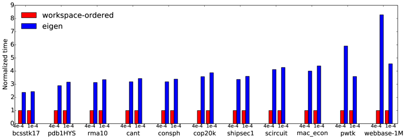
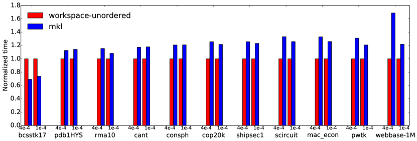
Figure 11 shows running times for sparse matrix multiplication for each matrix in Table 1 multiplied by a synthetic matrix of nonzero densities 1E-4 and 4E-4, using our fused workspace implementation. On average, Eigen is slower than our approach, which generates a variant of Gustavson’s matrix multiplication algorithm, by 4$\times$ and 3.6$\times$ respectively for the two sparsity levels. For the unsorted algorithm, we compare against Intel MKL, and find that our performance is 28% faster and 16% on average. The generated workspace algorithm is faster (by up to 68%) than MKL’s hand-optimized SpMM implementation in all but one case, which is 31% slower.

Table 2 breaks down the running times for the different codes for multiplying with a matrix of density 4E-4. Due to sorting, assembly times for the sorted algorithm are quite large; however, the compute time is occasionally faster than the unsorted compute time, due to improved locality when accumulating workspace entries into the result matrix. The fused algorithm is also faster when not using sorting, because otherwise the sort dominates the time (we use the standard C qsort).

7.3. Matricized Tensor Times Khatri-Rao Product

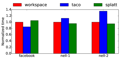
Matricized tensor times Khatri-Rao product (MTTKRP) is used to compute generalizations of SVD factorization for tensors in data analytics. The three-dimensional version takes as input a sparse 3-tensor and two matrices, and outputs a matrix. Figure 12 shows the results for our workspace algorithm on three input tensors, compared to taco and the hand-coded SPLATT library. We show only compute times, as the assembly times are negligible because the outputs are dense. We compare parallel single-socket implementations, using numactl to restrict execution to a single socket.

For the NELL-1 and NELL-2 tensors, the workspace algorithm outperforms the merge-based algorithm in taco and is within 5% of the hand-coded performance of SPLATT. On the smaller Facebook dataset, the merge algorithm is faster than both our implementation and SPLATT’s. That is, different inputs perform better with different algorithms, which demonstrates the advantage of being able to generate both versions of the algorithm.

7.4. Matricized Tensor Times Khatri-Rao Product with Sparse Matrices

It is useful to support MTTKRP where both the tensor and matrix operands are sparse (Smith et al., 2017a). If the result is also sparse, then the MTTKRP can be much faster since it only needs to iterate over nonzeros. The code is tricky to write, however, and cannot be generated by the current version of taco, although the prior merge-based theory supports it. In this section, we use a workspace implementation of sparse MTTKRP enabled by the workspace optimization. As far as we are aware, ours is the first implementation of an MTTKRP algorithm where all operands are sparse and the output is a sparse matrix. Because we have not implemented a parallel version of MTTKRP with sparse outputs, we perform this comparison with single-threaded implementations of both MTTKRP versions.

Figure 12. Matricized tensor times Khatri-Rao product (MTTKRP) running times, normalized to the workspace algorithm running time. MTTKRP is run in parallel using numactl to restrict execution to a single socket. Only compute times are shown; assembly times are negligible because the outputs are dense.

Figure 13. MTTKRP compute time as we vary the density of the matrix operands, for the three test tensors. We compare MTTKRP computed with a workspace when the matrix operands are passed in as dense matrices with a dense output against an implementation that takes sparse matrices as inputs and outputs a sparse matrix. In all cases, the tensor is passed in using a sparse format. This comparison uses single-threaded performance, as we have not implemented a parallel MTTKRP with sparse output.

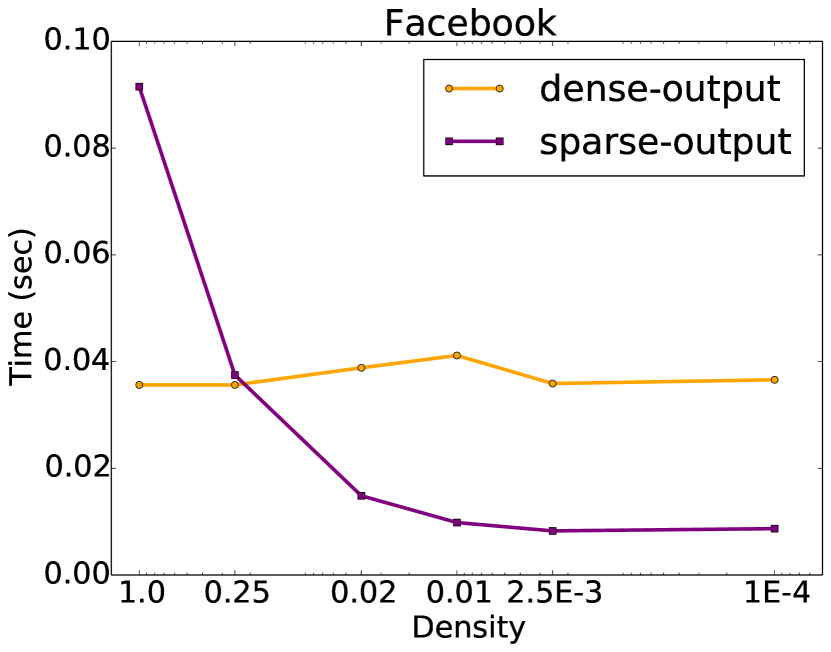
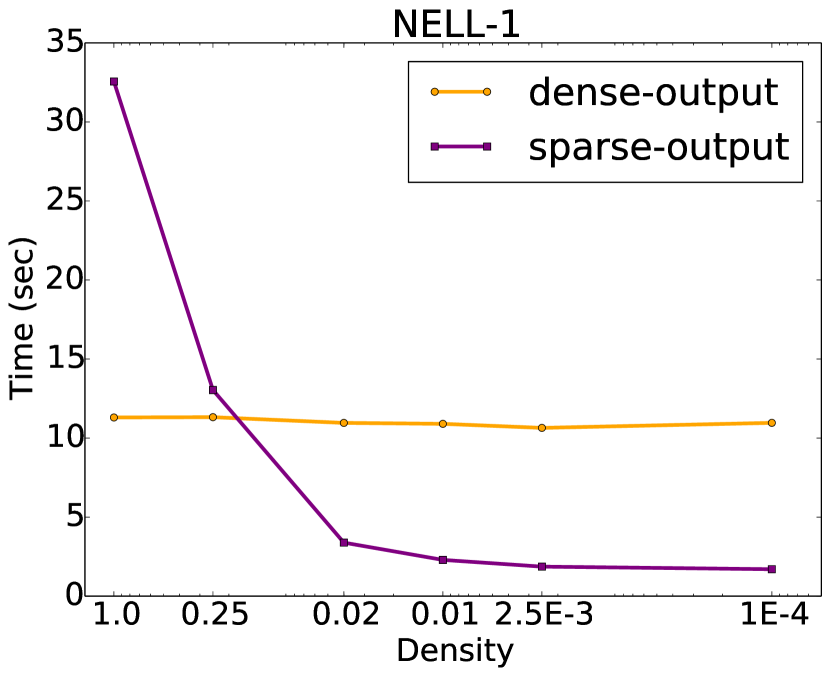
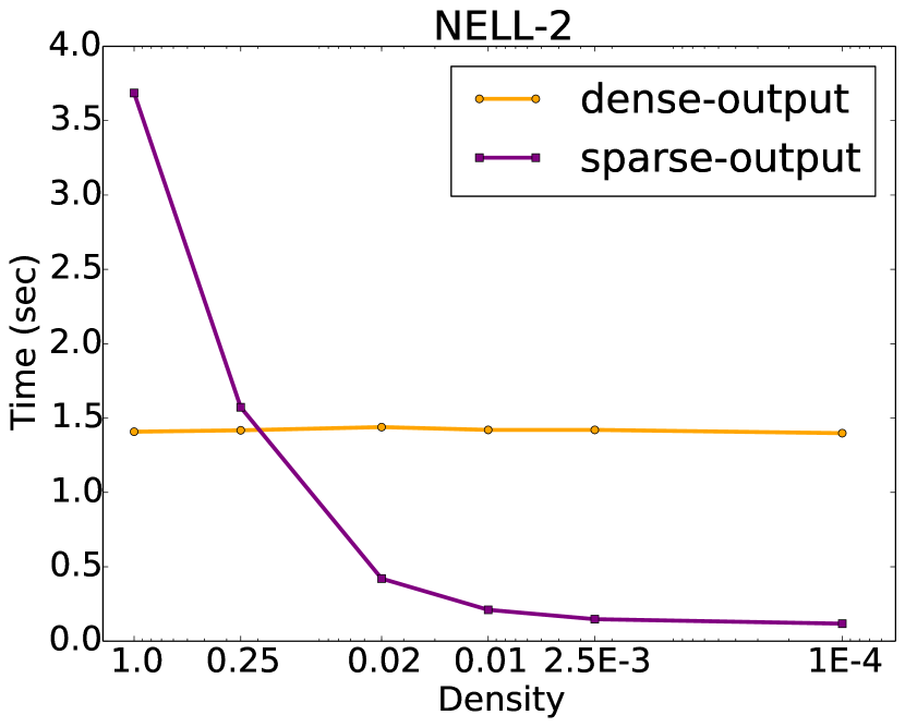
Which version is faster depends on the density of the sparse operands. Figure 13 shows experiments that compares the compute times for MTTKRP with sparse matrices against MTTKRP with dense matrices, as we vary the density of the randomly generated input matrices. Note that the dense matrix version should have the same performance regardless of sparsity and any variation is likely due to system noise. For each of the tensors, the crossover point is at about 25% nonzero values, showing that such a sparse algorithm can be faster even with only a modest amount of sparsity in the inputs. At the extreme, matrix operands with density 1E-4 can obtain speedups of 4.5–11$\times$ for our three test tensors.

Code	Assembly	Compute
taco binop	247	211
taco	190	182
workspace	190	93.3
Eigen		436
MKL		1141

Figure 14. Left: Scaling plot showing the time to assemble and compute $n$ matrix additions with Eigen, MKL, taco binary operations, a single multi-operand taco function, and workspaces. The matrices are described in Table 14. Right: Breakdown of sparse matrix addition time in ms for adding 7 matrices, for all codes The operands are randomly-generated sparse matrices of density 2.56E-02, 1.68E-03, 2.89E-04, 2.50E-03, 2.92E-03, 2.96E-02, 1.06E-02, respectively.

7.5. Sparse Matrix Addition

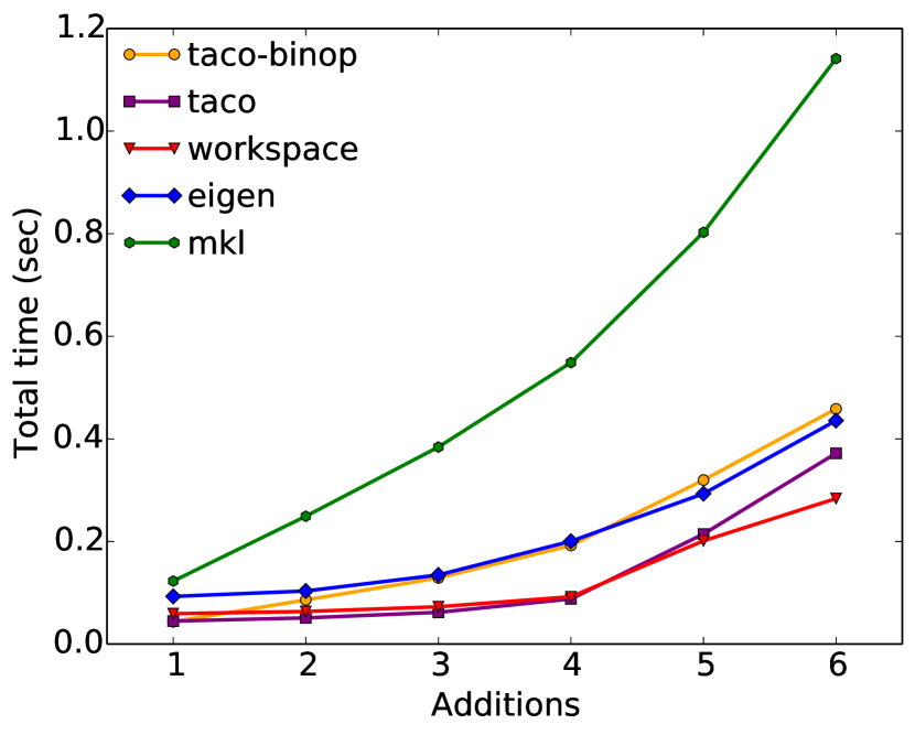
To demonstrate the utility of workspaces for sparse matrix addition (SpAdd), we show that the algorithm scales as we increase the number of operands. In Figure 14, we compare the workspace algorithm to taco using binary operations (as a library would be implemented), taco generating a single function for the additions, Intel MKL (using its inspector-executor SpAdd implementation), and Eigen. We pre-generate $k$ matrices with the target sparsities chosen uniformly randomly from the range [1E-4, 0.01] and always add in the same order and with the same matrices for each library.

The results of this experiment show two things. First, that the libraries are hampered by the restriction that they perform addition two operands at a time, having to construct and compute multiple temporaries, resulting in less performance than is possible using code generation. Even given this approach, taco is faster than Intel MKL by 2.8$\times$ on average, while Eigen and taco show competitive performance.

Secondly, the experiment shows the value of being able to produce both merge-based and workspace-based implementations of SpAdd. At up to four additions, the two versions are competitive, with the merge-based code being slightly faster. However, with increasing numbers of additions, the workspace code begins to outperform the taco implementation, showing an increasing gap as more operands are added. Table 14 breaks down the performance of adding 7 operands, separating out assembly time for the taco-based and workspace implementations. For this experiment, we reuse the matrix assembly code produced by taco to assemble the output, but compute using a workspace. Most of the time is spent in assembly, which is unsurprising, given that assembly requires memory allocations, while the computation performs only point-wise work without the kinds of reductions found in MTTKRP and SpMM.

8. Related Work

Related work is divided into work on tensor algebra compilation, work on manual workspace optimizations of matrix and tensor kernels, and work on general loop optimization.

There has been much work on optimizing dense matrix and tensor computations (Iverson, 1962; Wolfe, 1982; McKinley et al., 1996; Auer et al., 2006). Researchers have also worked on compilation and code generation of sparse matrix computations, starting with the work of Bik and Wijshoff (Bik and Wijshoff, 1993), the Bernoulli system (Kotlyar et al., 1997), and SIPR (Pugh and Shpeisman, 1999). Recently, Kjolstad et al. (2017) proposed a tensor algebra compilation theory that compiles tensor index notation on dense and sparse tensors. These sparse compilation approaches, however, did not generate sparse code with tensor workspaces to improve performance.

One use of the workspace optimization in loop nests, in addition to removing multi-way merge code and scatters into sparse results, is to split apart computation that may take place at different loop levels. This results in operations being hoisted to a higher loop nest. Loop invariant code motion has a long history in compilers, going back to the first FORTRAN compiler in 1957 (Backus, 1978). Recently, researchers have found new opportunities for removing redundancy in loops by taking advantage of high-level algebraic knowledge (Ding and Shen, 2017). Our workspace optimization applies to sparse tensor algebra and can remove loop reduncancies from sparse code with indirect-access loop bounds and many conditional branches.

The polyhedral model was originally designed to optimize dense loop nests with affine loop bounds and affine accesses into dense arrays. Sparse code, however, involves nested indirect array accesses. Recent work has to extend the polyhedral model to these situations (Strout et al., 2012; Belaoucha et al., 2010; Venkat et al., 2015; Venkat et al., 2016), using a combination of compile-time and runtime techniques, but the space of loop nests on nested indirect array accesses is complicated, and it difficult for compilers to determine when linear-algebraic optimizations are applicable to the operations that the code represents. Our workspace optimization applies to sparse tensor algebra at the concrete index notation level, before sparse code is generated, which makes it possible to perform aggressive optimizations and convenient to reason about legality.

The first use of dense workspaces for sparse matrix computations is Gustavson’s sparse matrix multiplication implementation, that we recreate with the workspace optimization in Figure 8 to produce the code in and Figure 1 (Gustavson, 1978). A workspace used for accumulating temporary values is referred to as an expanded real accumulator in (Pissanetzky, 1984) and as an abstract sparse accumulator data structure in (Gilbert et al., 1992). Dense workspaces and blocking are used to produce fast parallel code by Patwary et al. (Patwary et al., 2015). They also tried a hash map workspace, but report that it did not have good performance for their use. Furthermore, Buluç et al. use blocking and workspaces to develop sparse matrix-vector multiplication algorithms for the CSB data structure that are equally fast for $Ax$ and $A^{T}x$ (Buluç et al., 2009). Finally, Smith et al. uses a workspace to hoist loop-invariant code in their implementation of MTTKRP in the SPLATT library (Smith et al., 2015). We re-create this optimization with the workspace optimization in Figure 10 and show the resulting source code in Figure 10.

9. Conclusion

This paper presented the concrete index notation optimization language for describing how tensor index notation should execute and a workspace optimization that introduces workspaces to remove insertion into sparse results, conditionals, and to hoist loop-invariant computations. The optimization enables a new class of sparse tensor computations with sparse results and improves performance of other tensor computations to match state-of-the-art hand-optimized implementations. We believe the importance of workspaces will increase in the future as combining new tensor formats will require workspaces as glue. Furthermore, we believe the concrete index notation language can grow into a language for general tensor optimization, including loop tiling, strip-mining, and splitting. Combined with a scheduling language to command these concrete index notation transformations, the resulting system separates algorithm from schedule. This lets end users specify the computation they want, in tensor index notation, while the specification for how it should execute can be specified by performance experts, autotuning systems, machine learning, or heuristics.

References

- (1)
- Auer et al. (2006) Alexander A. Auer, Gerald Baumgartner, David E. Bernholdt, Alina Bibireata, Venkatesh Choppella, Daniel Cociorva, Xiaoyang Gao, Robert Harrison, Sriram Krishnamoorthy, Sandhya Krishnan, Chi-Chung Lam, Qingda Lu, Marcel Nooijen, Russell Pitzer, J. Ramanujam, P. Sadayappan, and Alexander Sibiryakov. 2006. Automatic code generation for many-body electronic structure methods: the tensor contraction engine. Molecular Physics 104, 2 (2006), 211–228.
- Backus (1978) John Backus. 1978. The history of FORTRAN I, II, and III. In History of programming languages I. ACM, 25–74.
- Bader and Kolda (2007) Brett W Bader and Tamara G Kolda. 2007. Efficient MATLAB computations with sparse and factored tensors. SIAM Journal on Scientific Computing 30, 1 (2007), 205–231.
- Belaoucha et al. (2010) Marouane Belaoucha, Denis Barthou, Adrien Eliche, and Sid-Ahmed-Ali Touati. 2010. FADAlib: an open source C++ library for fuzzy array dataflow analysis. Procedia Computer Science 1, 1 (May 2010), 2075–2084. https://doi.org/10.1016/j.procs.2010.04.232
- Bezanson et al. (2012) Jeff Bezanson, Stefan Karpinski, Viral B. Shah, and Alan Edelman. 2012. Julia: A Fast Dynamic Language for Technical Computing. (2012).
- Bik and Wijshoff (1993) Aart JC Bik and Harry AG Wijshoff. 1993. Compilation techniques for sparse matrix computations. In Proceedings of the 7th international conference on Supercomputing. ACM, 416–424.
- Buluç et al. (2009) Aydin Buluç, Jeremy T Fineman, Matteo Frigo, John R Gilbert, and Charles E Leiserson. 2009. Parallel sparse matrix-vector and matrix-transpose-vector multiplication using compressed sparse blocks. In Proceedings of the twenty-first annual symposium on Parallelism in algorithms and architectures. ACM, 233–244.
- Cichocki (2014) Andrzej Cichocki. 2014. Era of big data processing: A new approach via tensor networks and tensor decompositions. arXiv preprint arXiv:1403.2048 (2014).
- Davis (2006) Timothy A Davis. 2006. Direct methods for sparse linear systems. Vol. 2. Siam.
- Davis and Hu (2011) Timothy A. Davis and Yifan Hu. 2011. The University of Florida Sparse Matrix Collection. ACM Trans. Math. Softw. 38, 1, Article 1 (Dec. 2011).
- Ding and Shen (2017) Yufei Ding and Xipeng Shen. 2017. GLORE: Generalized Loop Redundancy Elimination Upon LER-notation. Proc. ACM Program. Lang. 1, OOPSLA, Article 74 (Oct. 2017), 28 pages. https://doi.org/10.1145/3133898
- Gilbert et al. (1992) John R Gilbert, Cleve Moler, and Robert Schreiber. 1992. Sparse matrices in MATLAB: Design and implementation. SIAM J. Matrix Anal. Appl. 13, 1 (1992), 333–356.
- Guennebaud et al. (2010) Gaël Guennebaud, Benoît Jacob, et al. 2010. Eigen v3. http://eigen.tuxfamily.org. (2010).
- Gustavson (1978) Fred G. Gustavson. 1978. Two Fast Algorithms for Sparse Matrices: Multiplication and Permuted Transposition. ACM Trans. Math. Softw. 4, 3 (1978).
- Hansen (1970) Per Brinch Hansen. 1970. The Nucleus of a Multiprogramming System. Commun. ACM 13, 4 (April 1970), 238–241. https://doi.org/10.1145/362258.362278
- Heath et al. (1991) Michael T Heath, Esmond Ng, and Barry W Peyton. 1991. Parallel algorithms for sparse linear systems. SIAM review 33, 3 (1991), 420–460.
- Hitchcock (1927) Frank L Hitchcock. 1927. The expression of a tensor or a polyadic as a sum of products. Studies in Applied Mathematics 6, 1-4 (1927), 164–189.
- Intel (2012) Intel. 2012. Intel math kernel library reference manual. Technical Report. 630813-051US, 2012. http://software.intel.com/sites/products/documentation/hpc/mkl/mklman/mklman.pdf.
- Iverson (1962) Kenneth E. Iverson. 1962. A Programming Language. Wiley.
- Kjolstad et al. (2017) Fredrik Kjolstad, Shoaib Kamil, Stephen Chou, David Lugato, and Saman Amarasinghe. 2017. The Tensor Algebra Compiler. Proc. ACM Program. Lang. 1, OOPSLA, Article 77 (Oct. 2017), 29 pages. https://doi.org/10.1145/3133901
- Knuth (1973) Donald Ervin Knuth. 1973. The art of computer programming: sorting and searching. Vol. 3. Pearson Education.
- Kolda and Bader (2009) Tamara G Kolda and Brett W Bader. 2009. Tensor decompositions and applications. SIAM review 51, 3 (2009), 455–500.
- Kotlyar et al. (1997) Vladimir Kotlyar, Keshav Pingali, and Paul Stodghill. 1997. A relational approach to the compilation of sparse matrix programs. In Euro-Par’97 Parallel Processing. Springer, 318–327.
- MATLAB (2014) MATLAB. 2014. version 8.3.0 (R2014a). The MathWorks Inc., Natick, Massachusetts.
- McKinley et al. (1996) Kathryn S McKinley, Steve Carr, and Chau-Wen Tseng. 1996. Improving data locality with loop transformations. ACM Transactions on Programming Languages and Systems (TOPLAS) 18, 4 (1996), 424–453.
- Möcks (1988) Joachim Möcks. 1988. Topographic components model for event-related potentials and some biophysical considerations. IEEE transactions on biomedical engineering 35, 6 (1988), 482–484.
- Patwary et al. (2015) Md. Mostofa Ali Patwary, Nadathur Rajagopalan Satish, Narayanan Sundaram, Jongsoo Park, Michael J Anderson, Satya Gautam Vadlamudi, Dipankar Das, Sergey G Pudov, Vadim O Pirogov, and Pradeep Dubey. 2015. Parallel efficient sparse matrix-matrix multiplication on multicore platforms. In International Conference on High Performance Computing. Springer, 48–57.
- Phan and Cichocki (2010) Anh Huy Phan and Andrzej Cichocki. 2010. Tensor decompositions for feature extraction and classification of high dimensional datasets. Nonlinear theory and its applications, IEICE 1, 1 (2010), 37–68.
- Pissanetzky (1984) Sergio Pissanetzky. 1984. Sparse Matrix Technology-electronic edition. Academic Press.
- Pugh and Shpeisman (1999) William Pugh and Tatiana Shpeisman. 1999. SIPR: A new framework for generating efficient code for sparse matrix computations. In Languages and Compilers for Parallel Computing. Springer, 213–229.
- Ragan-Kelley et al. (2012) Jonathan Ragan-Kelley, Andrew Adams, Sylvain Paris, Marc Levoy, Saman Amarasinghe, and Frédo Durand. 2012. Decoupling algorithms from schedules for easy optimization of image processing pipelines. (2012).
- Shashua and Levin (2001) Amnon Shashua and Anat Levin. 2001. Linear image coding for regression and classification using the tensor-rank principle. In Computer Vision and Pattern Recognition, 2001. CVPR 2001. Proceedings of the 2001 IEEE Computer Society Conference on, Vol. 1. IEEE, I–I.
- Smith et al. (2017a) Shaden Smith, Alec Beri, and George Karypis. 2017a. Constrained Tensor Factorization with Accelerated AO-ADMM. In Parallel Processing (ICPP), 2017 46th International Conference on. IEEE, 111–120.
- Smith et al. (2017b) Shaden Smith, Jee W. Choi, Jiajia Li, Richard Vuduc, Jongsoo Park, Xing Liu, and George Karypis. 2017b. FROSTT: The Formidable Repository of Open Sparse Tensors and Tools. (2017). http://frostt.io/
- Smith et al. (2015) Shaden Smith, Niranjay Ravindran, Nicholas Sidiropoulos, and George Karypis. 2015. SPLATT: Efficient and Parallel Sparse Tensor-Matrix Multiplication. In 2015 IEEE International Parallel and Distributed Processing Symposium (IPDPS). 61–70.
- Solomonik et al. (2014) Edgar Solomonik, Devin Matthews, Jeff R. Hammond, John F. Stanton, and James Demmel. 2014. A massively parallel tensor contraction framework for coupled-cluster computations. J. Parallel and Distrib. Comput. 74, 12 (Dec. 2014), 3176–3190. https://doi.org/10.1016/j.jpdc.2014.06.002
- Strout et al. (2012) Michelle Mills Strout, Geri Georg, and Catherine Olschanowsky. 2012. Set and Relation Manipulation for the Sparse Polyhedral Framework. In Languages and Compilers for Parallel Computing (Lecture Notes in Computer Science). Springer, Berlin, Heidelberg, 61–75. https://doi.org/10.1007/978-3-642-37658-0_5
- Tinney and Walker (1967) William F Tinney and John W Walker. 1967. Direct solutions of sparse network equations by optimally ordered triangular factorization. Proc. IEEE 55, 11 (1967), 1801–1809.
- Vasilache et al. (2018) Nicolas Vasilache, Oleksandr Zinenko, Theodoros Theodoridis, Priya Goyal, Zachary DeVito, William S. Moses, Sven Verdoolaege, Andrew Adams, and Albert Cohen. 2018. Tensor Comprehensions: Framework-Agnostic High-Performance Machine Learning Abstractions. (Feb. 2018). https://arxiv.org/abs/1802.04730
- Venkat et al. (2015) Anand Venkat, Mary Hall, and Michelle Strout. 2015. Loop and Data Transformations for Sparse Matrix Code. In Proceedings of the 36th ACM SIGPLAN Conference on Programming Language Design and Implementation (PLDI 2015). 521–532.
- Venkat et al. (2016) Anand Venkat, Mahdi Soltan Mohammadi, Jongsoo Park, Hongbo Rong, Rajkishore Barik, Michelle Mills Strout, and Mary Hall. 2016. Automating wavefront parallelization for sparse matrix computations. In Proceedings of the International Conference for High Performance Computing, Networking, Storage and Analysis. IEEE Press, 41.
- Wolfe (1982) Michael Joseph Wolfe. 1982. Optimizing Supercompilers for Supercomputers. Ph.D. Dissertation. University of Illinois at Urbana-Champaign, Champaign, IL, USA. AAI8303027.
- Wulf et al. (1974) W. Wulf, E. Cohen, W. Corwin, A. Jones, R. Levin, C. Pierson, and F. Pollack. 1974. HYDRA: The Kernel of a Multiprocessor Operating System. Commun. ACM 17, 6 (June 1974), 337–345. https://doi.org/10.1145/355616.364017
- Zhao (2014) Huasha Zhao. 2014. High Performance Machine Learning through Codesign and Rooflining. Ph.D. Dissertation. EECS Department, University of California, Berkeley.