Large scale distribution of mass versus light from Baryon Acoustic Oscillations:
Measurement in the final SDSS-III BOSS Data Release 12

Abstract

Baryon Acoustic Oscillations (BAOs) in the early Universe are predicted to leave an as yet undetected signature on the relative clustering of total mass versus luminous matter. This signature, a modulation of the relative large-scale clustering of baryons and dark matter, offers a new angle to compare the large scale distribution of light versus mass. A detection of this effect would provide an important confirmation of the standard cosmological paradigm and constrain alternatives to dark matter as well as non-standard fluctuations such as Compensated Isocurvature Perturbations (CIPs). The first attempt to measure this effect in the SDSS-III BOSS Data Release 10 CMASS sample remained inconclusive but allowed to develop a method, which we detail here and use to conduct the second observational search. When using the same model as in our previous study and including CIPs in the model, the DR12 data are consistent with a null-detection, a result in tension with the strong evidence previously measured with the DR10 data. This tension remains when we use a more realistic model taking into account our knowledge of the survey flux limit, as the data then privilege a zero effect. In the absence of CIPs, we obtain a null detection consistent with both the absence of the effect and the amplitude predicted in previous theoretical studies. This shows the necessity of more accurate data in order to prove or disprove the theoretical predictions.

1 Introduction

The imprint left by Baryon Acoustic Oscillations (BAOs), propagating in the baryon-radiation fluid before the time of recombination, is a powerful cosmological tool. The signature they left in the large scale distribution of mass was first detected in the 2dF Galaxy Redshift Survey (2dFGRS) (Percival et al., 2001; Eisenstein et al., 2005; Cole et al., 2005) and was more recently measured in WiggleZ (Blake et al., 2011) and the SDSS Data Release 12 (Anderson et al., 2014).

Another important signature of BAOs is the imprint they left on the clustering of light relative to mass. Indeed, the acoustic waves which propagated in the baryon-radiation fluid before the time of recombination were only felt by the baryonic matter and not followed by Dark Matter (DM). After recombination, in the absence of any radiation pressure, gravitational instability took over the distribution of baryons and the strong discrepancy between the location of the baryonic shell and the cold-dark-matter started fading away. However, the resulting scale-dependency of the ratio of baryonic matter to total matter contrasts, $\delta_{\rm b}/\delta_{\rm tot}$, should still be observable at present time. Detecting this scale-dependency would offer a new angle to compare the large scale distribution of light versus mass, an effort which dates back to the 1980s (Lahav, 1987; Erdoǧdu et al., 2006; Desjacques et al., 2016; Schmidt, 2016; Smith et al., 2017). Soumagnac et al. (2016) conducted a first search for this effect in the data from the Baryon Oscillation Spectroscopic Survey (BOSS) data release DR10.

Specifically, the scale-dependency of $\delta_{\rm b}/\delta_{\rm tot}$, imprinted by BAOs, is important for three reasons:

1. The detection of the effect would provide a direct measurement of a difference in the large-scale clustering of mass and light and a confirmation of the standard cosmological paradigm. It would help rule out alternative theories of gravity, specifically non-DM models such as MOND (Milgrom, 1994). The main evidence against such theories today is the data from the bullet cluster (Clowe et al., 2006). The measurement of the scale-dependency of $\delta_{\rm b}/\delta_{\rm tot}$ from BAOs, would provide evidence comparable to the bullet cluster, with the additional advantage that this effect happens on linear scales.

2. The amplitude of the effect would allow a calibration of the dependence of the characteristic mass-to-light ratio of galaxies on the baryon mass fraction of their large scale environment.

3. Soumagnac et al. (2016) showed that such a detection would also allow constraints to be placed on the amplitude of Compensated Isocurvature Perturbations (CIPs).

The measurement of the scale-dependency of $\delta_{\rm b}/\delta_{\rm tot}$ requires one to compare observable tracers of $\delta_{\rm tot}$ and $\delta_{\rm b}$. In this paper, we detail the approach by Soumagnac et al. (2016), an extension of the proposal by Barkana & Loeb (2011) (denoted BL11 in the rest of this paper) to use the number density $\delta_{\rm n}$ of galaxies as a tracer of the total matter density fluctuation $\delta_{\rm tot}$ and the absolute luminosity density of galaxies as a tracer of the baryonic density fluctuation $\delta_{\rm tot}$. In section 2, we remind and detail the main aspects of the model developed by BL11 and extended in Soumagnac et al. (2016). In section 3, we present our measurement of $\xi_{\rm L}$ and $\xi_{\rm n}$ from the SDSS-III BOSS Data Release 12 CMASS sample. Section 4.1 is dedicated to our model-fitting strategy. We then conclude on the significance of our detection with a model selection calculation, in section 4.2. We give concluding remarks in section 5.

2 The model

2.1 A model for $\delta_{\rm b}/\delta_{\rm tot}$

The number density fluctuations $\delta_{\rm n}$ are driven by the underlying total matter density fluctuation $\delta_{\rm tot}$, with a bias $b_{\rm n}$, which should be approximately constant on large scales.

$$\delta_{\rm n}=b_{\rm n}\cdot\delta_{\rm tot}$$ (1)

On the other hand, an area with a higher baryonic mass fraction $\delta_{\rm b}/\delta_{\rm tot}$ than average is expected to produce more stars per unit total mass, hence more luminous matter, and to result in galaxies with lower mass-to-light ratio. As a result, the luminosity-weighted density fluctuation, $\delta_{\rm L}$, provides a tracer of $\delta_{\rm b}$, the baryonic contribution to $\delta_{\rm tot}$.

Therefore scale-dependency of $\delta_{\rm b}/\delta_{\rm tot}$ induced by BAOs, should translate into a scale-dependency of $\delta_{\rm L}/\delta_{\rm tot}$. This being said, the mean luminosity of a given galaxy population relates to the baryonic content of the surrounding in a non-trivial way. The link between them is a combination of

1. the way in which the luminosity of a galaxy depends on the baryon fraction of the host halo,

2. the way in which the baryonic content of the host halo reflects the underlying baryonic contribution to the total matter density.

The luminosity density $\rho_{\rm L}$, for a given population of galaxies, is given by

$$\rho_{L}=n_{\rm gal}\left<L\right>$$ (2)

where $\left<L\right>$ is the mean absolute luminosity of the population of galaxies.

$\left<L\right>$ may also depend on $\delta_{\rm tot}$, through the merger history of the population of galaxies. We model this dependency with a different bias $b_{\rm n}+b_{\rm L;t}$:

$$\delta_{\rm L}=(b_{\rm n}+b_{\rm L;t})\cdot\delta_{\rm tot}$$ (3)

This would be right if $\left<L\right>$ only depended on the large scale matter density. However, $\left<L\right>$ also depends on the baryon fraction in the host halo, $f_{\rm b}$. Following BL11, we assume that $\left<L\right>\propto(f_{\rm b})^{b_{\rm L;f}}$, where $b_{\rm L;f}\approx 1.4$ is the bias factor of the luminosity density with respect to the halo baryon fraction. Hence equation 3 becomes

$$\delta_{\rm L}=(b_{\rm n}+b_{\rm L;t})\cdot\delta_{\rm tot}+b_{\rm L;f}\delta_{\rm f}$$ (4)

The link between the baryonic content of the halo $\delta_{\rm f}$ and the baryonic content of the surrounding $\delta_{\rm b}$ is complex because of the non-linearity of halo collapse. It is derived in BL11 as,

$$\delta_{\rm f}=\frac{A_{\rm r}}{\delta_{\rm c}}[r(k)-r_{\rm lss}]\delta_{\rm tot}\;,$$ (5)

where

• $r(k)$ is the fractional baryon deviation $r(k)=\delta_{\rm b}/\delta_{\rm tot}-1$, shown in figure 1 as a function of the scale k, and at various redshifts. $r(k)$ approaches a constant $r_{\rm lss}$ which depends on the redshift, on scales below the BAOs.

• $\delta_{\rm c}$ is the critical total matter density $\delta_{\rm tot}$ of the halo at which the critical density of collapse is independent of mass and is equal to $1.69$ in the Eistein-De Siter limit, valid over a wide range of redshifts, (Naoz & Barkana, 2007).

• $A_{\rm r}$ is a corrective amplification factor coming from the use of the linear $r(k)$ in the non-linear halo collapse problem, and is expected to be $A_{\rm r}\approx 3$, from simulations computed in BL11.

Hence, the final equation for $\delta_{\rm L}$ is

$$\delta_{\rm L}=(b_{\rm n}+b_{\rm L;t})\cdot\delta_{\rm tot}+b_{\rm L,\Delta}(r(k)-r_{\rm lss})\cdot\delta_{\rm tot}\;,$$ (6)

where $b_{\rm L,\Delta}$ is a bias factor measuring the overall dependence of galaxy luminosity and the underlying difference between the baryon and total density fluctuations and is predicted in BL11 to be around $b_{\rm L,\Delta}\approx 2.5$.

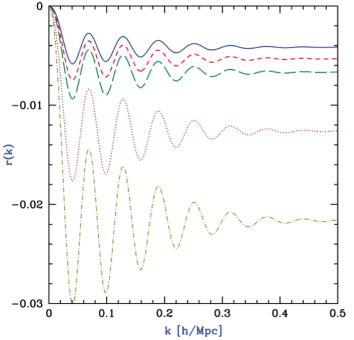
Figure 1: The fractional baryon derivation $r(k)=(\delta_{\rm b}/\delta_{\rm tot})-1$, as a function of the scale $k$, at various redshifts ($z=0$,$0.5$,$1$,$3$ and $6$ from top to bottom). Credit: BL11.

In BL11, the authors show that, in the case of a flux limited survey, both equations 1 and 6 must be slightly rethought. In such surveys, observed samples are limited by flux, or equivalently by luminosity if, for simplicity, we consider samples at a single redshift. The number of observable galaxies per unit of volume is given by

$$F(L)=\int_{L^{\prime}=L}^{\infty}\phi(L^{\prime})dL^{\prime}\;,$$ (7)

where $\phi$ is the luminosity function. The observed luminosity density of these galaxies becomes

$$\rho_{obs}=\left<L\right>F(L),$$ (8)

where the mean luminosity of the sample $\left<L\right>$ is now defined as

$$\left<L\right>=\frac{1}{F(L)}\int_{L^{\prime}=L}^{\infty}L^{\prime}\phi(L^{\prime})dL^{\prime}\;.$$ (9)

One can then show that equations 1 and 6 rewrite

$$\delta_{\rm n}=(b_{\rm n}+C_{\rm min}b_{\rm L;t})\delta_{\rm tot}+C_{\rm min}b_{\rm L,\Delta}[r(k)-r_{\rm lss}]\delta_{\rm tot}\;,$$ (10)

and

$$\delta_{\rm L}=\left(b_{\rm n}+(1+D_{\rm min})b_{\rm L;t}\right)\delta_{\rm tot}+b_{\rm L,\Delta}(1+D_{\rm min})[r(k)-r_{\rm lss}]\delta_{\rm tot}\;,$$ (11)

where $C_{\rm min}=\frac{L_{\rm min}\phi(L_{\rm min})}{F(L_{\rm min})}$ and $D_{\rm min}=\frac{L_{\rm min}}{\left<L\right>}C_{\rm min}$ with $\left<L\right>$ evaluated for $L=L_{\rm min}$.

The limit of a non flux-limitted survey corresponds to $C_{\rm min}=D_{\rm min}=0$. As noted in Barkana & Loeb (2011), in the opposite limit where $L_{min}>L_{*}$ (L_* is the characteristic galaxy luminosity where the power-law form of the luminosity function cuts off), we can approximately set $\phi(L)\propto e^{-L/L_{*}}$ and then

$$C_{\rm min}=\frac{L_{\rm min}}{L_{*}}\;\;\;\;,\;\;\;\;D_{\rm min}=\frac{C_{\rm min}L_{\rm min}}{L_{\rm min}+L_{*}}\,.$$ (12)

2.2 Compensated Isocurvature Perturbations

The measurement of the relation between dark matter and baryons, is related to the search for Compensated Isocurvature Perturbations (CIPs) (Grin et al., 2014). Measurements of primordial density perturbations are consistent with adiabatic initial conditions, for which the ratios of neutrino, photon, baryon and DM number densities are initially spatially constant. On the one hand, the simplest inflationary models predict adiabatic fluctuations (Guth & Pi, 1982; Linde, 1982). On the other, hand, more complex inflationary scenarii (Brandenberger, 1994; Linde, 1984; Axenides et al., 1983) predict fluctuations on the relative number densities of different species, known as Isocurvature Perturbations (IPs). CMB temperature anisotropies limit the contribution of both baryons and DM to the total isocurvature perturbation amplitude. CIPs are perturbations in the baryons density $\delta_{\rm b}$ which are compensated for by corresponding fluctuations in the DM $\delta_{DM}$, so that the total density is unchanged.

Such fluctuations are hard to detect, since the effects of gravity measurable by galaxy surveys (including galaxy numbers), only depend on the total density. Galaxy clusters gas fractions observations (Holder et al., 2010) have lead to a weak constraints of the CIP’s. $21$cm absorption observations are expected to allow a slightly better constraint of such perturbations (Gordon & Pritchard, 2009). Under the standard assumption of a scale-invariant power spectrum for this field, equations 11 and 10 are modified to

$$\delta_{\rm n}=(b_{\rm n}+C_{\rm min}b_{\rm L;t})\delta_{\rm tot}+C_{\rm min}b_{\rm L,\Delta}[(r(k)-r_{\rm lss})\delta_{\rm tot}+\delta_{CIP}]\;,$$ (13)

$$\delta_{\rm L}=(b_{\rm n}+(1+D_{\rm min})b_{\rm L;t})\delta_{\rm tot}+(1+D_{\rm min})b_{\rm L,\Delta}[(r(k)-r_{\rm lss})\delta_{\rm tot}+\delta_{CIP}]\;,$$ (14)

where $\delta_{CIP}$ is a separate field that is uncorrelated with $\delta_{\rm tot}$. With the method presented in this paper, we hope to improve the $10^{-2}$ current constraint on the amplitude of a scale invariant CIPs power spectrum (Grin et al., 2014).

2.3 Model in terms of correlation function

Equations 13 and 14 provide a model for the tracers of the quantities of interest $\delta_{\rm b}$ and $\delta_{\rm tot}$. However, the observable quantities in galaxy surveys are the two point statistics of such tracers, namely the power spectrum or the two-point correlation functions (2PCF). We reformulate the observational proposal of BL11 in terms of the 2PCF, defined as

$$\xi({\bf x},{\bf y})\equiv\int\frac{d^{3}{\bf k}}{(2\pi)^{3/2}}\frac{d^{3}{\bf k^{\prime}}}{(2\pi)^{3/2}}\langle\delta({\bf k})\delta({\bf k^{\prime}})\rangle e^{i{\bf k}\cdot{\bf x}}e^{i{\bf k}\cdot{\bf y}}=\frac{1}{2\pi^{2}}\int k^{2}P(k)j_{0}(ks)dk\;,$$ (15)

where $P(k)$ is the power spectrum defined by $\left<\delta(k)\delta(k^{\prime})\right>\equiv P(k)\delta^{D}(k-k^{\prime})$. In real space, and assuming $|r(k)-r_{\rm lss}|<<1$, equation 10 and equation 11 translate into the following,

$$\xi_{\rm n}=B_{\rm n,t}^{2}\cdot\xi_{\rm tot}+2B_{\rm n,t}B_{\rm n,\Delta}\cdot\xi_{\rm add}+B_{\rm n,\Delta}^{2}B_{\rm CIP}\cdot\hat{\xi}_{\rm CIP}\;,$$ (16)

and

$$\xi_{\rm L}=B_{\rm L,t}^{2}\cdot\xi_{\rm tot}+2B_{\rm L,t}B_{\rm L,\Delta}\cdot\xi_{\rm add}+B_{\rm L,\Delta}^{2}B_{\rm CIP}\cdot\hat{\xi}_{\rm CIP}\;.$$ (17)

with

$$B_{\rm n,t}=b_{\rm n}+C_{\rm min}b_{\rm L;t}$$ (18)

$$B_{\rm n,\Delta}=C_{\rm min}b_{\rm L,\Delta}$$ (19)

$$B_{\rm L,t}=b_{\rm n}+(1+D_{\rm min})b_{\rm L;t}$$ (20)

$$B_{\rm L,\Delta}=(1+D_{\rm min})b_{\rm L,\Delta}=\frac{1+D_{\rm min}}{C_{\rm min}}B_{\rm n,\Delta}$$ (21)

A key issue in the modeling of these correlation functions is to understand how they evolve with time. In section 2.4, we adopt a simplistic approach and model $\xi_{\rm tot}$ and $\xi_{\rm add}$ with a linear perturbation theory. We then correct for the non-linearity of the clustering of galaxies in section 2.5.

2.4 Linear-regime matter correlation

In order to model the $\xi_{\rm tot}$ and $\xi_{\rm add}$ components of equations 16 and 17, we first compute a linear power spectrum $P(k)$ and a linear fractional baryon deviation $r(k)$ using CAMB (Lewis et al., 2000). We assume the same fiducial $\Lambda$CDM+GR, flat cosmological model with $\Omega_{m}=0.274$, $h=0.7$, $\Omega_{b}h^{2}=0.0224$, $n_{s}=0.95$ and $\sigma_{8}=0.8$, matching that used by the BOSS collaboration in Anderson et al. (2014). P(k) and r(k) are computed for the median redshifts of the sample we use, namely the CMASS sample of the BOSS DR12 release (Ahn et al. 2012, 2014; Alam et al. 2015; see section 3).

To model $\xi_{CIP}$, we make the standard assumption that the power spectrum of the CIP field is of the form $P_{CIP}(k)=A_{CIP}k^{-3}$ (Grin et al., 2014). Since the corresponding correlation function

$$\xi_{CIP}(s)=\frac{1}{2\pi^{2}}\int k^{2}P_{CIP}(k)\cdot j_{0}(ks)dk=\frac{A_{CIP}}{2\pi^{2}}\int\frac{j_{0}(ks)}{k}dk$$

diverges, we compute the integration from $k=10^{-4}h/Mpc$, which is also the minimum value of the CAMB linear power spectrum we use to model $\xi_{\rm tot}$.

2.5 Corrections to the linear correlation functions

The matter correlation $\xi_{\rm tot}$ predicted by linear perturbation theory does not exactly describe the clustering of galaxies. Nonlinear gravitational collapse and redshift distortions modify galaxy clustering relative to that of the linear-regime matter correlations, changing the shape of the correlation function. In particular, according to linear perturbation theory, the acoustic signature increases in amplitude but the characteristic scale imprinted in the early universe remains unaltered, whereas non linear growth of structure leads to a shift of the acoustic peak. In Soumagnac et al. (2016), the authors accounted for two systematic effects due to nonlinear clustering: damping of the BAO peak and mode coupling.

2.5.1 Damping

Simulations have shown that nonlinear structure formation and, to a lesser extent, redshift distortions erase the higher harmonics of the acoustic oscillations. This degrades the measurement of the acoustic scale. This effect is accounted for by “damping” the linear theoretical BAO on small scales. The damping term is often approximated by a Gaussian smoothing (Percival et al., 2010). The corrected correlation function is given by

$$\xi_{\rm tot}(s)=\xi(s)\otimes e^{-(k_{*}\cdot s)^{2}}=\frac{1}{2\pi^{2}}\int k^{2}P(k)e^{-(k_{*}\cdot k)^{2}}j_{0}(ks)dk\;.$$ (22)

The damping is also applied to $\xi_{\rm add}$ and $\xi_{CIP}$.

2.5.2 Mode coupling

Mode coupling generates additional oscillations that are out of phase with those in the linear spectrum, leading to shifts in the scales of oscillation nodes defined with respect to a smooth spectrum. When Fourier transformed, these out-of-phase oscillations induce percent-level shifts in the acoustic peak of the two-point correlation function. The corresponding correction to the damped linear correlation function is given in Crocce & Scoccimarro (2008), as:

$$\xi_{\rm tot}(s)=\xi(s)\otimes e^{-(k_{*}\cdot s)^{2}}+A_{\rm MC}\xi^{\prime}(s)\xi^{(1)}(s)\;,$$ (23)

where $\xi(s)$ denotes the linear correlation function of equation 15 and

$$\xi^{(1)}(s)=\int\frac{d^{3}k}{k}P(k)j_{1}(ks)\;,$$ (24)

where $j_{1}$ is the first order Bessel function.

2.5.3 Systematics

The systematic effects of BOSS data are investigated in Ross et al. (2012a) and essentially cause a constant shift in $\xi$. A simple way to account for systematics that would affect differently $\xi_{\rm L}$ and $\xi_{\rm n}$ is to add a constant to the model in equation 17. Thus, equation 17 becomes

$$\xi_{\rm L}=B_{\rm L,t}^{2}\cdot\xi_{\rm tot}+2B_{\rm L,t}B_{\rm L,\Delta}\cdot\xi_{\rm add}+B_{\rm L,\Delta}^{2}B_{\rm CIP}\cdot\hat{\xi}_{\rm CIP}\\ +B_{\rm sys,L}\;.$$

2.5.4 Full model equations

Our final model equations, also given in the supplemental material of Soumagnac et al. (2016) are:

$$\xi_{\rm n}=B_{\rm n,t}^{2}\cdot\xi_{\rm tot}+2B_{\rm n,t}B_{\rm n,\Delta}\cdot\xi_{\rm add}+B_{\rm n,\Delta}^{2}B_{\rm CIP}\cdot\hat{\xi}_{\rm CIP}$$ (25)

$$+B_{\rm sys,n}\;,$$

and

$$\xi_{\rm L}=B_{\rm L,t}^{2}\cdot\xi_{\rm tot}+2B_{\rm L,t}B_{\rm L,\Delta}\cdot\xi_{\rm add}+B_{\rm L,\Delta}^{2}B_{\rm CIP}\cdot\hat{\xi}_{\rm CIP}$$ (26)

$$+B_{\rm sys,L}\;.$$

where

$$\xi_{\rm tot}(s)=\xi(s)\otimes e^{-(k_{*}\cdot s)^{2}}+A_{\rm MC}\xi^{\prime}(s)\xi^{(1)}(s)\;,$$

$$\xi_{\rm add}(s)=\frac{1}{2\pi^{2}}\left(\int k^{2}[r(k)-r_{\rm lss}]P(k)j_{0}(ks)dk\right)\otimes e^{-(k_{*}\cdot s)^{2}}\;,$$

$$\xi_{\rm CIP}(s)\equiv B_{\rm CIP}\cdot\hat{\xi}_{\rm CIP}(s)=\frac{B_{\rm CIP}}{2\pi^{2}}\left(\int\frac{j_{0}(ks)}{k}dk\right)\otimes e^{-(k_{*}\cdot s)^{2}}\;,$$

where $\otimes$ denotes convolution, $\xi(s)$ is the linear correlation function (eq. 3 of the main text), and

$$\xi^{(1)}(s)=\int\frac{d^{3}k}{k}P(k)j_{1}(ks)\;.$$

Thus, our full set of parameters is $\theta=\{B_{\rm n,t},B_{\rm L,t},B_{\rm n,\Delta},B_{\rm L,\Delta},B_{\rm CIP},B_{\rm sys,n},B_{\rm sys,L},A_{\rm MC},k_{*}\}$.

In order to compute the oscillatory integral $\xi_{\rm tot}$, $\xi_{\rm add}$ and $\xi_{CIP}$, we wrote a Python wrapper for the fftlog code from Hamilton (2000).

2.6 Previous results

In this section we summarize the results of the measurement by Soumagnac et al. (2016), which used the DR10 data and are brought for comparision throughout the paper.

When allowing CIPS in the model, i.e., $B_{\rm CIP}\neq 0$, the authors obtained evidence at $3.2\sigma$ of the relative clustering signature. The $1\sigma$ range of $1.1<B_{\rm L,\Delta}<2.8$ was consistent with the prediction of BL11 of $B_{\rm L,\Delta}\approx 2.6$ (predicted along with two assumptions: (1) $B_{\rm n,\Delta}\approx 0$ - an assumption that may be wrong here, as explained in section 2.7 - and (2) $B_{\rm n,t}$ and $B_{\rm L,t}$ approximately equal). In addition, the best-fit value of $B_{\rm CIP}$ is $2.3\times 10^{-3}$, with a $2\sigma$ upper limit of $B_{\rm CIP}=6.4\times 10^{-2}$, which is within an order of magnitude of the best existing limits noted previously. A full tabulation of the DR10 best-fit parameters is given in the Supplemental Material of Soumagnac et al. (2016).

However, the DR10 results were not robust enough for making strong claims. When modeling the data without allowing for CIPs (i.e., setting $B_{\rm CIP}=0$), the evidence for a detection of non-zero $B_{\rm L,\Delta}$ goes away. The authors obtained a null detection consistent with both the absence of the effect and the BL11 prediction.

2.7 Luminosity function and constraint on $B_{\rm L,\Delta}$

Within the model by BL11, the parameters and in particular the ratio $B_{\rm L,\Delta}/B_{\rm n,\Delta}$ depend on the flux limit of the survey. Here, we use equation 21 and our knowledge of the BOSS sample to derive an additional constraint on the parameters of the model. The BOSS DR12 CMASS sample data are in the regime of rare, bright galaxies, well into the exponential tail of the luminosity function. Specifically, the flux limit in the $i$ band is $17.5<i<19.9$, which translates into $L_{\rm min}\approx 8.4$ $10^{10}L_{\rm\odot}$. With $L_{*}\approx 2$ $10^{10}L_{\rm\odot}$ (Sparke & Gallagher, 2006), we are well in the limit where $L_{\rm min}\gg L_{*}$ and we can substitute equation 12 into equation 21, which gives

$$B_{\rm L,\Delta}/B_{\rm n,\Delta}\approx 1.0\;,$$ (27)

We checked that our results are not very sensitive to the exact value of $L_{*}$. In all the following, we fit the data with two models: (1) a model with unconstrained parameters $B_{\rm L,\Delta}$ and $B_{\rm n,\Delta}$, as in Soumagnac et al. (2016) and (2) a more realistic model, reflecting our knowledge of the sample flux limit, where $B_{\rm L,\Delta}=B_{\rm n,\Delta}$ as in equation 27.

3 Measurement

3.1 The BOSS DR12 sample

In this analysis, we use the public data from the Sloan Digital Sky Survey’s (SDSS-III) Baryon Oscillation Spectroscopic Survey (BOSS), data release 12 (DR1, Alam et al. 2015). The SDSS (York et al. 2000), divided into SDSS I, II (Abazajian et al. 2009), and III (Eisenstein et al. 2011), used a drift-scanning mosaic CCD camera (Gunn et al. 1998) to image over one third of the sky (14,555 square degrees) in five photometric bands [$u,g,r,i,z$] (Fukugita et al. 1996; Doi et al. 2010) to a limiting magnitude of $r\approx$ 22.5 using the dedicated 2.5-m Sloan Telescope located at Apache Point Observatory in New Mexico.

BOSS is primarily a spectroscopic survey, which is designed to obtain spectra and redshifts for $\sim$1.35 million galaxies over an extragalactic footprint covering $\sim$10,000 square degrees. These galaxies are selected from the SDSS DR8 imaging. Together with these galaxies, 160 000 quasars and approximately 100 000 ancillary targets are being observed. The method by which the spectra are obtained (Smee et al. 2013) ensures a homogeneous data set with a high redshift completeness of more than 97$\%$ over the full survey footprint. Redshifts are extracted from the spectra using the methods described in Bolton et al. (2012). A summary of the survey design appears in Eisenstein et al. (2011), and a full description is provided in Dawson et al. (2013).

Two classes of galaxies were selected by BOSS to be targeted for spectroscopy using SDSS DR8 imaging. The “LOWZ” algorithm is designed to select red galaxies at $z<0.45$ from the SDSS DR8 imaging data. While the “CMASS” sample is designed to be approximately stellar-mass-limited above z = 0.45.

In our previous work we considered only the CMASS sample from DR10, in this work we use DR12 data which is $\sim 50\%$ larger in angular sky coverage. We leave the analysis using the LOWZ sample for future developments of this work. The details of the catalogue are provided in table 1.

	CMASS
redshift range	$0.43<z<0.7$
effective redshift	0.57
effective area	9376 deg2
effective volume	4.70 Gpc3
number of galaxies	800,853

Table 1: Summary of the data samples used. The effective volume is calculated using our fiducial model and the amplitude of the matter power spectrum at the BAO scale $P_{0}=10,000~{}h^{-3}$Mpc³.

3.2 Estimator & Computation

Several practical problems inhibit our ability to accurately measure the 2PCF of the galaxy distribution, as defined in equation 15. The discreet sampling by individual galaxies of the smooth density field leads to shot noise on small scales. Other difficulties arise from the irregular shape of galaxy surveys in angular sky coverage, due to dust extinction, bright stars, tracking of the telescope, etc. We must use statistical estimators which can deal with such problems (see Percival (2007), for a review of correlation function practicalities and Kerscher et al. 2000, for a review of correlation estimators). In this work, the two-point correlation functions $\xi_{n}$ and $\xi_{L}$, are computed using the optimal Landy-Salay estimator (Landy & Szalay, 1993) which requires the creation of a catalog of random positions.

$$\xi(r)=\frac{DD-2DR+RR}{RR},$$ (28)

where DD, DR and RR represent the number of normalised pairs of points at a particular separation, $r$, between the data (D) and a random catalogue (R).

In practice, this computation involves counting of the number of weighted pairs separated by $r$ and normalised by the total number of possible weighted pairs in the galaxy sample, the random sample and the cross counts between galaxy-random points. In our analysis. These counts are computed using an efficient tree-based, parallel, search algorithm called KSTAT. The code is based upon the structure known as “kd-trees” which is a way of organizing a set of data in k-dimensional space in such a way that once built, any query requesting a list of points in a neighbourhood can be answered quickly without going through every single point.

3.3 Measurement of $\xi_{n}(r)$ and $\xi_{L}(r)$

For both the number density correlation function $\xi_{n}$ and the luminosity-weighted correlation function $\xi_{L}$, we use the published DR12 data and random catalogs, including both the radial FKP weights and the angular systematic weights.

The FKP weights (Feldman et al., 1994) are applied to all galaxy and random points according to we assign to each data point a radial weight of $w_{FKP}=1/[1+n(z)P_{0}]$, where n(z) is the radial number density of galaxies and $P_{0}$(=10,000) is the amplitude of the power spectrum near the BAO scale.

Each galaxy is assigned a weight according to,

$$w_{i}=w_{FKP,i}.w_{sys,i}(w_{rf,i}+w_{fb,i}-1),$$ (29)

where $w_{sys}$ accounts for the correlations between galaxies and stellar density, while $w_{rf}$ and $w_{fb}$ upweights galaxies according to the missed redshifts of neighbouring targeted galaxies due to redshift failure and fibre collision. More details on these weights can be found in Ross et al. (2012b); Reid et al. (2016). The computation of the luminosity-weighted correlation function $\xi_{L}$ requires several steps which are detailed in the next sections.

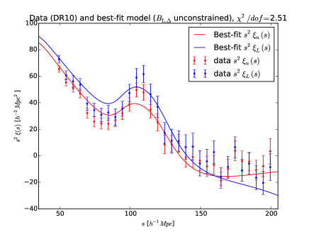
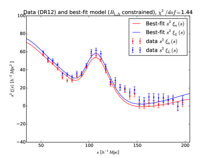
Figure 2: Our measurement of the correlation functions $\xi_{\rm n}$ and $\xi_{\rm L}$ (1) with an unconstrained $B_{\rm L,\Delta}$, using the CMASS-DR10 sample (top left) and the CMASS-DR12 sample (top right) and (2) with $B_{\rm L,\Delta}=B_{\rm n,\Delta}$ using the CMASS-DR12 sample (lower panel). A quantitative comparison of all three cases is given in section 4.1.2 and section 4.1.3.

3.3.1 Absolute magnitude and absolute luminosity

We calculate the two-point correlation function of the absolute luminosity density fluctuations, $\xi_{L}$, using the same estimator and algorithms for $\xi_{n}$, and weighting each object with its absolute luminosity. The absolute luminosity is calculated using the $i$ and $g$ bands photometric data, from the CMASS DR12 catalogs. We first compute the absolute magnitudes, using a combination of the “cmodel” magnitude parameter, referred to as $m_{cm}$, and the extinction parameter, $e$:

$$M_{\rm abs}=m_{cm}-e-(5log_{10}(D_{L})+25)-K_{Corr}\;,$$ (30)

where the luminosity distance $D_{L}$ (in Mpc) is linked to the comoving distance $D_{M}$ via $D_{L}=(1+z)\cdot D_{M}$. The $m_{cm}$ magnitude is a parameter in the DR12 catalogs derived from the composite flux $F_{composite}=f\cdot F_{dev}+(1-f)\cdot F_{exp}$ which is the best fitting linear combination of the exponential fit and the de Vaucouleurs fit in each band.

The parameter $e$ encapsulates the extinction correction, i.e. the account for the absorption and scattering of electromagnetic radiation by dust and gas between the observed galaxies and us. It has been computed following Schlegel et al. (1998).

The magnitude is also k-corrected, $K_{Corr}$, to convert the partial flux collected in the given band into the equivalent rest frame band. $K_{Corr}$ is obtained from the fitting formulae of Chilingarian et al. (2010).

The absolute luminosities are then computed using

$$L_{\rm abs}=10^{-(M_{\rm abs}-M_{\rm sun})/2.5}\;,$$ (31)

where $M_{\rm sun}=4.83$ is the absolute magnitude of the sun.

3.3.2 Correlation functions

Since the published DR12 random catalog does not include the photometric data necessary to compute $\xi_{\rm L}$, we create one by merging the right ascension and declination information from the available random catalog, with the redshift from the data catalog and the absolute luminosity computed from the data catalog, as explained above.

Our measurements of $\xi_{\rm L}$ and $\xi_{\rm n}$ are shown in figure 2, together with the previous DR10 measurement by Soumagnac et al. (2016) and our best-fit model, as detailed in the next sections.

3.4 Covariance matrix

The fitting procedure that we describe in section 4.1 requires that we estimate the covariance matrix for our measurement. Since the uncertainties of the measurements of $\xi_{\rm n}(r)$ and $\xi_{\rm L}(r)$ at a given point are correlated, we compute the full covariance matrix for the joint measurement of $\xi_{\rm n}(r)$ and $\xi_{\rm L}(r)$, as in Soumagnac et al. (2016). We use a Jackknife (JK) resampling technique, as in Scranton et al. (2002). We split the SDSS area into $N_{JK}$ approximately equal area regions (within 10% error). We then calculate each correlation function removing one area at a time, and generate our full covariance matrix as

$$C_{ij}=\frac{N-1}{N}\sum^{N_{JK}}_{k=1}\Delta^{k}_{i}\Delta^{k}_{j},$$ (32)

where the sum is over $N_{jk}$ JK samples and,

$$\Delta^{k}_{i}={[\xi^{k}(i)-\bar{\xi}(i)]},$$ (33)

where $\xi^{k}(i)$ is the 2PCF of the i-th bin in the k-th JK sample. We compute the joint covariance matrix for $\xi_{\rm n}$ and for $\xi_{\rm L}$, using 4096 Jackknife samples. This technique differs from the method adopted by the BOSS collaboration, where 600 mock catalogs were produced and used to estimate the covariance matrix for the fit. The mocks are described in Manera et al. (2013) and the full procedure they adopted to compute the covariance matrix is described in Percival et al. (2014). The reason we adopt a different approach is that we need to calculate the full covariance matrix for the joint measurement of $\xi_{\rm n}$ and $\xi_{\rm L}$. The mock produced by BOSS do not include any photometric information which would allow us to calculate the luminosity-weighted correlation function. In Soumagnac et al. (2016), the authors used the covariance matrix computed by BOSS as a way to check the consistency of this approach.

The full covariance matrix is shown in figure 3. It is far from being diagonal, or even block-diagonal, which shows the importance of fitting $\xi_{\rm n}$ and $\xi_{\rm L}$ jointly.

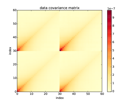
Figure 3: Our measurement of the joint covariance matrix using the CMASS-DR12 sample. It is not diagonal: the uncertainties on $\xi_{\rm n}$ and $\xi_{\rm L}$ are correlated, which underlines the importance of performing a joint fit of $\xi_{\rm n}$ and $\xi_{\rm L}$.

4 Results

We explored the two different cases presented in section 2.6 and section  2.7, namely a model with an unconstrained parameter $B_{\rm{L,\Delta}}$ and a model with a more realistic constraint $B_{\rm{L,\Delta}}=B_{\rm{n,\Delta}}$. We applied to both cases the methodology developed in Soumagnac et al. (2016) - which we present here in further details - to determine whether we detect a scale-dependent bias of the luminosity correlation function in the DR12 data, i.e. a non zero value of $B_{\rm L,\Delta}$.

4.1 Model Fitting

4.1.1 Formalism and computation

We adopt the terminology of Hogg et al. (2010), defining a generative model (a parametrized quantitative description of a statistical procedure that could reasonably have generated the data) and an objective scalar to be optimized. We assume that the only reason that our data point deviate from the model described by equations 25 and 26 is an offset in the $\xi$ direction, drawn from a gaussian distribution of zero mean and known variances $\sigma_{\xi}$. We wish to get the set of parameters $\theta=\{B_{\rm n,t},B_{\rm L,t},B_{\rm n,\Delta},B_{\rm CIP},B_{\rm sys,n},B_{\rm sys,L},A_{\rm MC},k_{*}\}$ which maximizes the probability of our model $\mathcal{M}$ given the data $\mathcal{D}$, i.e. the posterior probability distribution $Pr(\theta|\{\mathcal{D},\mathcal{M}\})$. Bayes’ theorem relates it to the likelihood $\mathcal{L}\equiv Pr(\mathcal{D}|\theta,\mathcal{M})$, via the prior $\pi\equiv Pr(\mathcal{D}|\mathcal{M},\theta)$:

$$Pr(\theta|\{\mathcal{D},\mathcal{M}\})=\frac{Pr(\mathcal{D}|\{\theta,\mathcal{M}\})\cdot Pr(\theta|\mathcal{M})}{Pr(\mathcal{D}|\mathcal{M})}=\frac{\mathcal{L}\cdot\pi}{E}\;,$$ (34)

where the evidence $E=Pr(\mathcal{D}|\mathcal{M})$ is the probability of getting the data $\mathcal{D}$, given the model $\mathcal{M}$ and can be seen as the likelihood averaged over all the possible parameters within a model.

Within the framework of a model-fitting approach, the evidence is seen as a marginalization constant and is ignored, since it does not affect the result of the optimization of the objective scalar. This is no longer true when adopting a model selection approach to our problem, as will be discussed in section 4.2. The likelihood of our generative model is :

$$\mathcal{L}\propto\exp\left[-\frac{1}{2}R^{T}\cdot C^{-1}\cdot R\right]$$ (35)

where ${\bf R}={\bf Y}-{\bf AX}$, and $C^{-1}$ is the inverse covariance matrix of the data ${\bf Y}$. We apply the following uniform (not “informative”) priors for the nine parameters of our model (the same as in Soumagnac et al. 2016):

• $B_{\rm n,t}\in[0,5]$

• $B_{\rm L,t}\in[0,5]$

• $B_{\rm n,\Delta}\in[-10,10]$

• $B_{\rm sys,L}\in[-0.01,0.01]$

• $B_{\rm sys,n}\in[-0.0015,0.0015]$

• $k_{*}\in[0,10]$

• $A_{\rm MC}\in[0,6]$

• $B_{\rm CIP}\in[-0.3,0.3]$

• $B_{\rm L,\Delta}\in[-10,10]$ (only in the case described in section 4.1.2)

We believe this is a conservative choice of priors. The priors on $B_{\rm L,\Delta}$ and $B_{\rm CIP}$ are intentionally taken to be broad. The priors on $B_{\rm sys,L}$ and $B_{\rm sys,n}$ are based on a study (Ross et al., 2012a) of the potential systematic effects in the BOSS data; this limit effectively allows a systematic contribution that is up to 3 times as large as the systematic contribution to $\xi_{\rm n}$ found in BOSS. The priors on $B_{\rm n,t}$, $k_{*}$ and $A_{\rm MC}$ are taken to be consistent with previous works on the BOSS data (Crocce & Scoccimarro, 2008; Anderson et al., 2012, 2014).

In the case of a not informative prior, the optimisation of the likelihood function corresponds to the maximum of the posterior distribution, i.e. the maximum a posteriori value. The problem then becomes to estimate the uncertainties on the maximum a posteriori value of each parameter, i.e. obtain the distribution of parameters that is consistent with our data, and to be able to marginalise over it to get the distribution of each parameter. This is made possible by Monte Carlo Markov Chain (MCMC) sampling. We used the multimodal nested sampling algorithm, MultiNest (Feroz & Hobson, 2008) to sample from the posterior probability distribution, and quote the uncertainties based on the $16^{th}$, $50^{th}$, and $84^{th}$ percentiles of the samples in the marginalised distributions, corresponding to $1\sigma$ in the case of a gaussian.

We consider two cases, corresponding to the presence or absence of CIPs. In Figures 2 and 4, we show the data and best fits for the correlation functions $r^{2}\xi_{\rm n}$ and $r^{2}\xi_{\rm L}$, and for a key quantity, their difference $r^{2}(\xi_{\rm L}-\xi_{\rm n})$.

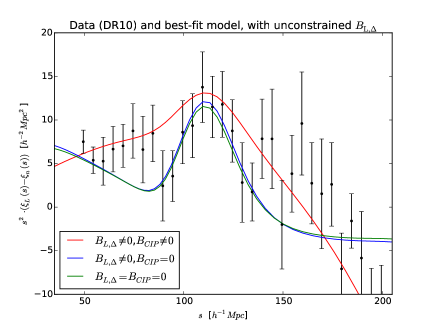
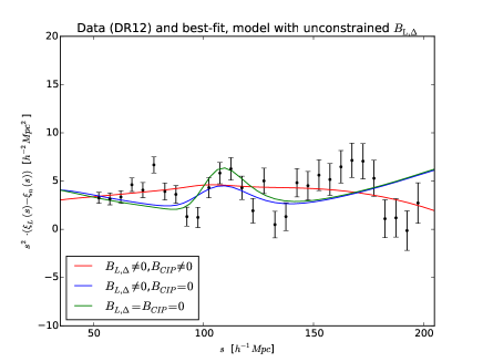
Figure 4: Our measurement of the difference $\xi_{\rm L}-\xi_{\rm n}$ (times $s^{2}$). The red line corresponds to our full model, the blue line corresponds to a model with $B_{\rm CIP}=0$, and the green line corresponds to a model with $B_{\rm CIP}=B_{\rm L,\Delta}=0$. The top panels show the data and best fit in the unconstrained case, using the CMASS-DR10 sample as in Soumagnac et al. 2016 (left) and the CMASS-DR12 sample (right). The lower panel shows the more realistic case where $B_{\rm L,\Delta}=B_{\rm n,\Delta}$, using the CMASS-DR12 sample. A quantitative comparison of all three cases is given in section 4.1.2 and section 4.1.3.

4.1.2 Unconstrained $B_{\rm{L,\Delta}}$

In figure 5 and figure 6, we show the two dimensional projections of the posterior probability distributions obtained by fitting the model from Soumagnac et al. (2016) (i.e. with unconstrained $B_{\rm{L,\Delta}}$) to the DR12 CMASS data. More specifically, Figure 5 corresponds to the case $B_{\rm CIP}\neq 0$ and figure 6 to the case $B_{\rm CIP}=0$. The value corresponding to the $16^{th}$, $50^{th}$, and $84^{th}$ percentiles of the samples in the marginalised distributions, i.e. the median value and the $1\sigma$ values (in the case of a gaussian) values are shown in table 2. The best fits to the data are shown and can be compared to the DR10 result in the top left panel of figure 4.

When CIPs are included in the model, i.e. when $B_{\rm CIP}\neq 0$, the $1\sigma$ range of $-0.91<B_{\rm L,\Delta}<0.74$ is consistent with zero, and in tension with the prediction of BL11 of $B_{\rm L,\Delta}\approx 2.6$ predicted along with the expectations of $B_{\rm n,\Delta}\approx 0$ (this assumption is likely not verified here, as discussed in section  2.7, but this does not affect our result since we did not assume it), and $B_{\rm n,t}$ and $B_{\rm L,t}$ approximately equal. This is an important difference from the result of Soumagnac et al. (2016), where the authors obtained evidence at $3.2\sigma$ of $B_{\rm L,\Delta}>0.4$ (and evidence that $|B_{\rm L,\Delta}|>0.4$ at $3.7\sigma$) when allowing CIPs, which was an indication of the effect we search for. In addition, our best-fit value of $B_{\rm CIP}$ is $2.7\times 10^{-3}$, with a $1\sigma$ upper limit of $B_{\rm CIP}=3.6\times 10^{-2}$, similar to the $3.7\times 10^{-2}$ upper limit provided by the DR10 data in Soumagnac et al. (2016) and within an order of magnitude of the best existing limits noted previously.

In the absence of CIPs, i.e. when $B_{\rm CIP}$ is set to zero, $B_{\rm L,\Delta}$ is less constrained. In this case, the $1\sigma$ range $-5.8<B_{\rm L,\Delta}<4.6$ is consistent with both zero and the BL11 prediction and similar to the $[-2.8,7.6]$ range computed with the DR10 data.

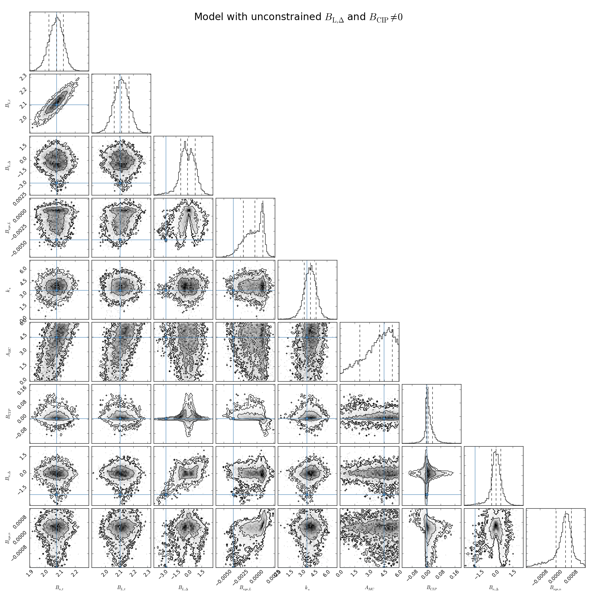
Figure 5: Joint fit of $\xi_{\rm n}$ and $\xi_{\rm L}$, unconstrained $B_{\rm L,\Delta}$ and $B_{\rm CIP}\neq 0$: all the one and two dimensional projections of the posterior probability distributions of the parameters,{$B_{\rm n,t}$,$B_{\rm L,t}$,$B_{\rm n,\Delta}$,$B_{\rm L,\Delta}$,$B_{\rm CIP}$,$B_{\rm sys,n}$,$B_{\rm sys,L}$,$A_{\rm MC}$,$k_{*}$}, in the case where $B_{\rm L,\Delta}$ is unconstrained, using the CMASS-DR12 sample. This quickly demonstrates all of the covariances between parameters.The contours correspond to the $1\sigma$, $2\sigma$ and $3\sigma$ percentiles. The blue line corresponds to the maximum likelihood value of each parameter, which is also the maximum a posteriori value (m.a.p.). The dashed lines show the $1\sigma$ percentile of the marginalized distributions.

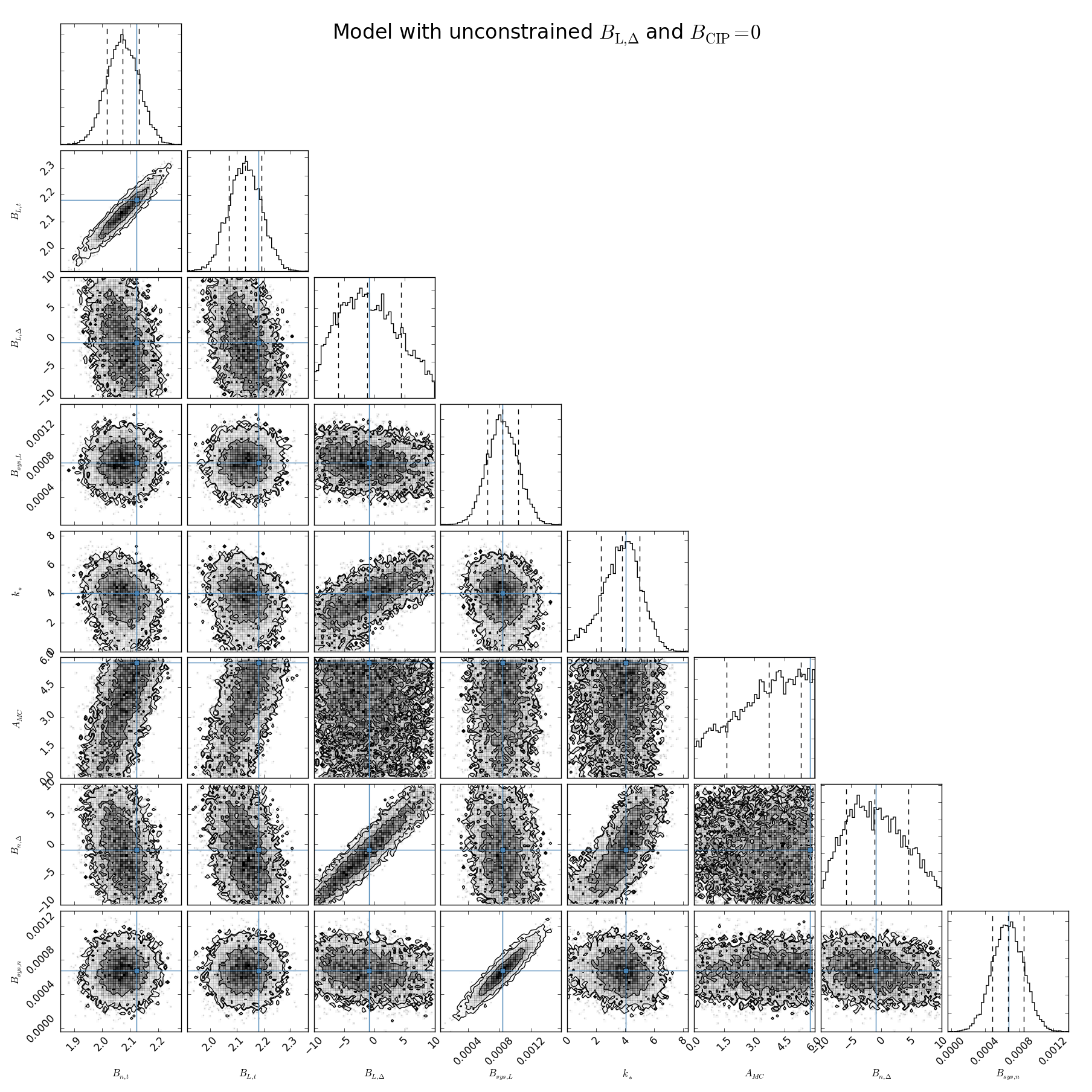
Figure 6: Joint fit of $\xi_{\rm n}$ and $\xi_{\rm L}$, unconstrained $B_{\rm L,\Delta}$ and $B_{\rm CIP}=0$: all the one and two dimensional projections of the posterior probability distributions of the parameters,{$B_{\rm n,t}$,$B_{\rm L,t}$,$B_{\rm n,\Delta}$,$B_{\rm L,\Delta}$,$B_{\rm CIP}$,$B_{\rm sys,n}$,$B_{\rm sys,L}$,$A_{\rm MC}$,$k_{*}$}, in the case where $B_{\rm L,\Delta}$ is unconstrained, using the CMASS-DR12 sample. This quickly demonstrates all of the covariances between parameters.The contours correspond to the $1\sigma$, $2\sigma$ and $3\sigma$ percentiles. The blue line corresponds to the maximum likelihood value of each parameter, which is also the maximum a posteriori value (m.a.p.). The dashed lines show the $1\sigma$ percentile of the marginalized distributions.

4.1.3 More realistic model with $B_{\rm{L,\Delta}}=B_{\rm{n,\Delta}}$

In figure 7 and figure 8, we show the two dimensional projections of the posterior probability distributions obtained by fitting a model where $B_{\rm L,\Delta}=B_{\rm n,\Delta}$ to the DR12 CMASS data. Figure 7 corresponds to the case $B_{\rm CIP}\neq 0$ and figure 8 to the case $B_{\rm CIP}=0$. A full tabulation of our best-fit parameters is shown in table 3. The best fits to the data are shown in figure 2 and figure 4 and can be compared to the DR10 result.

When CIPs are included in the model, i.e. when $B_{\rm CIP}\neq 0$, the $1\sigma$ range $-0.183<B_{\rm n,\Delta}<0.168$ is consistent with zero, and is in tension with the prediction in BL11 of $B_{\rm L,\Delta}\approx 2.6$, predicted along with the expectations of $B_{\rm n,\Delta}\approx 0$, (this latter assumption is likely not verified here, as discussed in section 2.7) and $B_{\rm n,t}$ and $B_{\rm L,t}$ approximately equal (which is indeed included in our model through the constraint $B_{\rm L,\Delta}=B_{\rm n,\Delta}$). $B_{\rm CIP}$, in this case, is less constrained, with a $1\sigma$ range $-0.105<B_{\rm CIP}<0.183$.

In the absence of CIPs, i.e. when $B_{\rm CIP}$ is set to zero, $B_{\rm n,\Delta}$ is less constrained and the $1\sigma$ range $-6.0<B_{\rm n,\Delta}<4.0$ is consistent with both zero and the BL11 prediction for $B_{\rm L,\Delta}$.

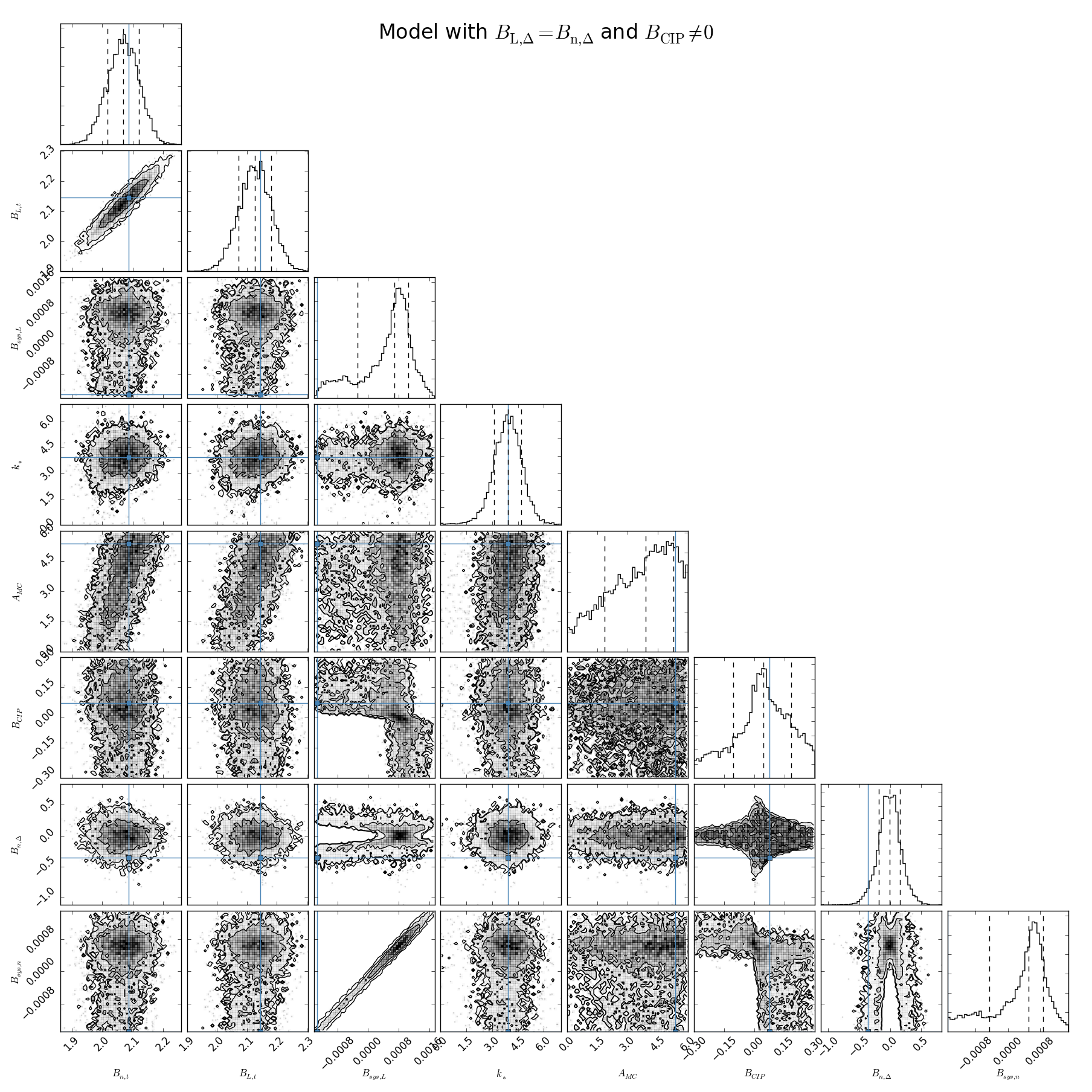
Figure 7: Joint fit of $\xi_{\rm n}$ and $\xi_{\rm L}$, with the constrain $B_{\rm L,\Delta}=B_{\rm n,Delta}$ and $B_{\rm CIP}\neq 0$: all the one and two dimensional projections of the posterior probability distributions of the parameters,{$B_{\rm n,t}$,$B_{\rm L,t}$,$B_{\rm n,\Delta}$,$B_{\rm CIP}$,$B_{\rm sys,n}$,$B_{\rm sys,L}$,$A_{\rm MC}$,$k_{*}$}, in the case where $B_{\rm L,\Delta}=B_{\rm n,\Delta}$ is unconstrained, using the CMASS-DR12 sample. This quickly demonstrates all of the covariances between parameters.The contours correspond to the $1\sigma$, $2\sigma$ and $3\sigma$ percentiles. The blue line corresponds to the maximum likelihood value of each parameter, which is also the maximum a posteriori value (m.a.p.). The dashed lines show the $1\sigma$ percentile of the marginalized distributions.

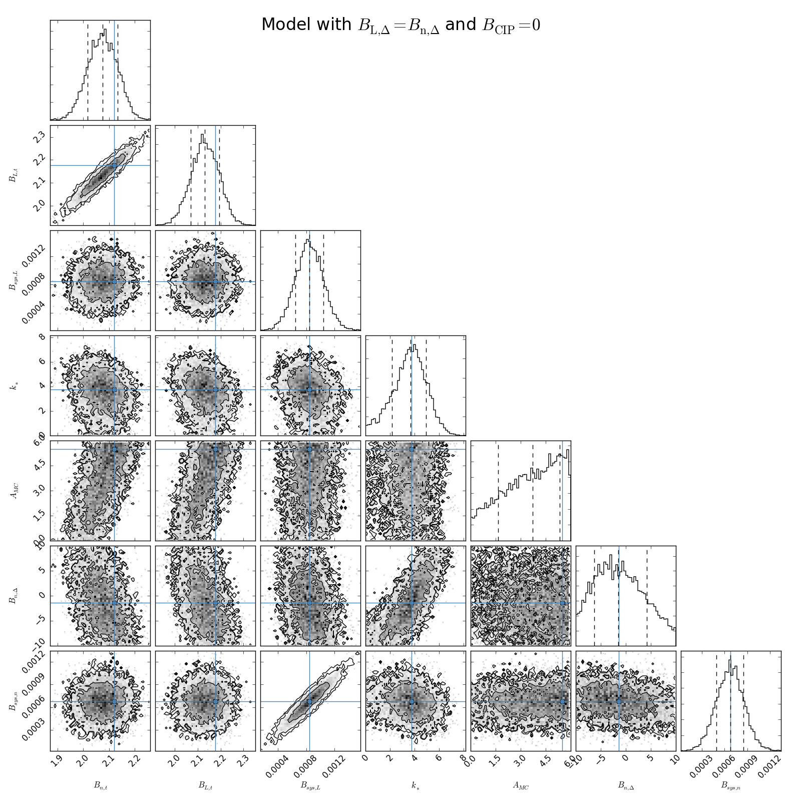
Figure 8: Joint fit of $\xi_{\rm n}$ and $\xi_{\rm L}$, with the constrain $B_{\rm L,\Delta}=B_{\rm n,Delta}$ and $B_{\rm CIP}=0$: all the one and two dimensional projections of the posterior probability distributions of the parameters,{$B_{\rm n,t}$,$B_{\rm L,t}$,$B_{\rm n,\Delta}$,$B_{\rm CIP}$,$B_{\rm sys,n}$,$B_{\rm sys,L}$,$A_{\rm MC}$,$k_{*}$}, in the case where $B_{\rm L,\Delta}=B_{\rm n,\Delta}$ is unconstrained, using the CMASS-DR12 sample. This quickly demonstrates all of the covariances between parameters.The contours correspond to the $1\sigma$, $2\sigma$ and $3\sigma$ percentiles. The blue line corresponds to the maximum likelihood value of each parameter, which is also the maximum a posteriori value (m.a.p.). The dashed lines show the $1\sigma$ percentile of the marginalized distributions.

	$B_{\rm CIP}\neq 0$			$B_{\rm CIP}=0$
Parameter	med.	max.	$68.2\%$-range	med.	max.	$68.2\%$-range
$B_{\rm n,t}$	$2.08$	$2.08$	$[2.03,2.12]$	$2.08$	$2.12$	$[2.02,2.13]$
$B_{\rm L,t}$	$2.12$	$2.10$	$[2.06,2.17]$	$2.13$	$2.18$	$[2.07,2.19]$
$B_{\rm L,\Delta}$	$-0.15$	$-2.66$	$[-0.91,0.74]$	$-1.00$	$-0.83$	$[-5.79,4.58]$
$B_{\rm sys,L}\times 10^{3}$	$-0.24$	$-3.57$	$[-2.02,0.91]$	$0.85$	$0.84$	$[0.65,1.05]$
$k_{*}$	$3.98$	$3.56$	$[3.26,4.71]$	$3.84$	$4.03$	$[2.34,5.01]$
$A_{\rm MC}$	$4.08$	$4.48$	$[2.04,5.34]$	$3.78$	$5.75$	$[1.68,5.34]$
$B_{\rm CIP}\times 10^{2}$	$1.26$	$0.27$	$[-0.06,3.57]$	$-$	$-$	$-$
$B_{\rm n,\Delta}$	$0.0484$	$-1.87$	$[-0.37,0.47]$	$-1.00$	$-0.89$	$[-5.79,4.59]$
$B_{\rm sys,n}\times 10^{4}$	$5.10$	$-15.0$	$[0.31,8.10]$	$6.80$	$6.72$	$[4.97,8.50]$

Table 2: Results of the model fitting, when using the CMASS sample and a model with unconstrained $B_{\rm L,\Delta}$ (i.e. the same model as in Soumagnac et al. 2016), for two configurations of the models: {$B_{\rm CIP}\neq 0,B_{\rm L,\Delta}\neq 0$} and {$B_{\rm CIP}=0,B_{\rm L,\Delta}\neq 0$}. The table shows the maximum likelihood value, the median, and $68.2\%$ confidence range for each parameter, computed using the marginalised posterior distributions obtained with the Multinest code.

	$B_{\rm CIP}\neq 0$			$B_{\rm CIP}=0$
Parameter	med.	max.	$68.2\%$-range	med.	max.	$68.2\%$-range
$B_{\rm n,t}$	$2.07$	$2.09$	$[2.02,2.12]$	$2.08$	$2.12$	$[2.02,2.14]$
$B_{\rm L,t}$	$2.13$	$2.15$	$[2.07,2.18]$	$2.13$	$2.18$	$2.07,2.19]$
$B_{\rm sys,L}\times 10^{3}$	$0.698$	$-1.33$	$[-0.251,1.05]$	$0.845$	$0.846$	$[0.661,1.04]$
$k_{*}$	$3.93$	$3.91$	$[3.16,4.7]$	$3.67$	$3.76$	$[2.2,4.97]$
$A_{\rm MC}$	$3.9$	$5.36$	$[1.86,5.28]$	$3.72$	$5.47$	$[1.68,5.34]$
$B_{\rm CIP}$	$0.048$	$0.0743$	$[-0.105,0.183]$	$-$	$-$	$-$
$B_{\rm n,\Delta}$	$-0.00765$	$-0.358$	$[-0.183,0.168]$	$-1.40$	$-1.42$	$[-6.2,4.2]$
$B_{\rm sys,n}\times 10^{4}$	$5.39$	$-15$	$[-4.48,8.97]$	$6.83$	$6.77$	$[4.97,8.56]$

Table 3: Results of the model fitting, when using the CMASS sample and a model with $B_{\rm L,\Delta}=B_{\rm n,\Delta}$, for two configurations of the models: {$B_{\rm CIP}\neq 0,B_{\rm L,\Delta}\neq 0$} and {$B_{\rm CIP}=0,B_{\rm L,\Delta}\neq 0$}. The table shows the maximum likelihood value, the median, and $68.2\%$ confidence range for each parameter, computed using the marginalised posterior distributions obtained with the Multinest code.

4.2 Model selection

To determine whether we detect a scale-dependent bias of the luminosity correlation function requires answering the following question: do the data support the inclusion of a non-zero parameter $B_{\rm L,\Delta}$? Rather than a question of parameter estimation (i.e. the determination of the most probable values for the extra parameters within the context of a single model), this is a question of model comparison between two models $\mathcal{M}$, with or without $B_{\rm L,\Delta}$. The parameter space $\Theta=\{B_{\rm n,t},B_{\rm L,t},B_{\rm n,\Delta},B_{\rm CIP},B_{\rm sys,n},B_{\rm sys,L},A_{\rm MC},k_{*}\}\equiv\{\phi,\psi\}$ is partitioned into the common parameters, $\phi=\{B_{\rm n,t},B_{\rm L,t},B_{\rm CIP},B_{\rm sys,n},B_{\rm sys,L},A_{\rm MC},k_{*}\}$, and the extra parameter $\psi=\{B_{\rm n,\Delta}\}$, describing the scale-dependent bias. The two models are nested, as defined in Verde et al. (2013).

Within a Bayesian framework Verde et al. (2013), the key quantity for comparing them is the Evidence (or model-averaged likelihood), $E=\int Pr(\theta|\mathcal{M})Pr(\mathcal{D}|\theta,\mathcal{M})d\theta$.

Our aim is to confront our degree of belief in the two different models $\mathcal{M}_{B_{\rm L,\Delta}\neq 0}$ and $\mathcal{M}_{B_{\rm L,\Delta}=0}$ in the light of the data, i.e. to compare $Pr(\mathcal{M}_{B_{\rm L,\Delta}\neq 0}|\mathcal{D})$ and $Pr(\mathcal{M}_{B_{\rm L,\Delta}=0}|\mathcal{D})$. Developing each term with Bayes’ theorem $Pr(\mathcal{M}|\mathcal{D})=Pr(\mathcal{D}|\mathcal{M})\cdot Pr(\mathcal{M})/Pr(\mathcal{D})$, we can write

$$\frac{Pr(\mathcal{M}_{B_{\rm L,\Delta}\neq 0}|\mathcal{D})}{Pr(\mathcal{M}_{B_{\rm L,\Delta}=0}|\mathcal{D})}=\frac{Pr(\mathcal{D}|\mathcal{M}_{B_{\rm L,\Delta}\neq 0})\cdot Pr(\mathcal{M}_{B_{\rm L,\Delta}\neq 0})}{Pr(\mathcal{D})}\cdot\frac{Pr(\mathcal{D})}{Pr(\mathcal{D}|\mathcal{M}_{B_{\rm L,\Delta}=0})\cdot Pr(\mathcal{M}_{B_{\rm L,\Delta}=0})}\;.$$ (36)

Since we do not have any prior preference toward one of the models, $\frac{Pr(\mathcal{M}_{B_{\rm L,\Delta}\neq 0})}{Pr(\mathcal{M}_{B_{\rm L,\Delta}=0})}$ is typically set to $1$ and the above ratio simplifies to

$$\frac{Pr(\mathcal{M}_{B_{\rm L,\Delta}\neq 0}|\mathcal{D})}{Pr(\mathcal{M}_{B_{\rm L,\Delta}=0}|\mathcal{D})}=\frac{E_{B_{\rm L,\Delta}\neq 0}}{E_{B_{\rm L,\Delta}=0}}\;.$$ (37)

The ratio of the evidences can be calculated using the multimodal nested sampling algorithm, MultiNest (Feroz & Hobson, 2008) and are all shown in table 4 for the CMASS sample.We use the slightly modified Jeffreys’ scale (Jeffrey, 1961; Kass & Raftery, 1995; Verde et al., 2013) shown in the appendix in table 5, which classifies Evidence ratios from ”not worth a bare mention” to “highly significant”, to interpret these values.

In the unconstrained case, i.e. within the model used by Soumagnac et al. (2016), the results are as follows. (1) When including CIPs in the model, the evidence ratio $\ln(E_{B_{\rm L,\Delta}\neq 0}/E_{B_{\rm L,\Delta}=0})=-1.04\pm 0.21$ corresponds to no evidence toward a non-zero $B_{\rm L,\Delta}$ over a zero effect. (2) In the absence of CIPs (i.e., when setting $B_{\rm CIP}=0$), the data strongly privilege $B_{\rm L,\Delta}\neq 0$, i.e. the presence of the effect we search for. This result is the opposite of the DR10 result presented in Soumagnac et al. (2016), where a strong evidence toward a non-zero $B_{\rm L,\Delta}\neq 0$ was measured when $B_{\rm CIP}\neq 0$ and disappeared in the absence of CIPs.

In the constrained case, i.e. when adding the more realistic constraint $B_{\rm L,\Delta}=B_{\rm n,\Delta}$ to the model by Soumagnac et al. (2016), the calculation of the evidence ratio leads to different conclusions. (1) In the presence of CIPs, the data privilege a zero $B_{\rm L,\Delta}$. The evidence ration $\ln(E_{B_{\rm L,\Delta}\neq 0}/E_{B_{\rm L,\Delta}=0})=-2.56\pm 0.20$ corresponds - according to the Jeffrey’s table 5 shown in the appendix- to “substantial” evidence for $B_{\rm L,\Delta}=0$. (2) In the absence of CIPs, the evidence for $B_{\rm L,\Delta}=0$ goes away: like in the DR10 analysis, the data do not privilege the effect we search for over the $B_{\rm L,\Delta}=0$ case.

	Unconstrained case	Constrained case
		($B_{\rm L,\Delta}=B_{\rm n,\Delta}$)
$B_{\rm CIP}\neq 0$	$-57.88\pm 0.11$	$-57.08\pm 0.10$
$B_{\rm L,\Delta}\neq 0$
$B_{\rm CIP}\neq 0$	$-56.84\pm 0.10$	$-54.52\pm 0.10$
$B_{\rm L,\Delta}=0$
$B_{\rm CIP}=0$	$-56.18\pm 0.10$	$-54.83\pm 0.10$
$B_{\rm L,\Delta}\neq 0$
$B_{\rm CIP}=0$	$-65.95\pm 0.11$	$-54.75\pm 0.10$
$B_{\rm L,\Delta}=0$

Table 4: Logarithm of the Bayesian evidence calculated with the multimodal nested sampling algorithm, MultiNest (Feroz & Hobson, 2008), using the CMASS sample.

5 Conclusion

We have compared the large scale distribution of mass and light, through measurement of the number-weighted and luminosity-weighted correlation functions $\xi_{\rm n}$ and $\xi_{\rm L}$, in the CMASS sample of DR12, the latest and last public data release from the SDSS-III Baryon Oscillation Spectroscopic Survey (BOSS). We have detailed the method for the detection, with a data set containing 3-D positions and photometry, of the modulation of the large scales ratio of baryonic matter to total matter ($\delta_{b}/\delta_{\rm tot}$), from BAOs. Within the framework of a model presented in Barkana & Loeb (2011) (BL11), which we have reformulated and specified, this modulation is characterised by a parameter, $B_{\rm L,\Delta}$, which we have measured in the BOSS CMASS DR12 data.

When compensated isocurvature perturbations (CIPs) are included in the model, the DR12 result is in tension with the strong evidence toward the effect we search for, which was observed in DR10. Indeed, the DR12 data is consistent either with a null detection - when using the same model as in Soumagnac et al. 2016 - or slightly privilege a model with no effect - when adding to the model an additional constraint that reflects our knowledge of the survey flux limit. If we do not include CIPs in the models and use our knowledge of the survey flux limit, we obtain a null detection of the effect, consistent with both $B_{\rm L,\Delta}=0$, and the theoretical $B_{\rm L,\Delta}$ predicted in previous theoretical studies.

As noted in Soumagnac et al. (2016), disentangling the various effects at stake is difficult. On the one hand, the model of equations 25 and 26 shows that any ability to set a limit on CIPs depends on a definitive detection of non-zero $B_{\rm L,\Delta}$ (and/or $B_{\rm n,\Delta}$). Conversely, the presence of a significant CIP term in the fit affects the range of $B_{\rm L,\Delta}$ and $B_{\rm n,\Delta}$ values. Trying to measure two novel effects (one of them expected but with an uncertain amplitude, the other highly speculative) when they are entangled is tricky. Another difficulty comes from the fact that $\hat{\xi}_{\rm CIP}$ has a smooth shape (in contrast with BAO-scale features in $\xi_{\rm tot}$ and $\xi_{\rm add}$), and such a slowly-varying term may more easily be emulated by systematic effects; we note that standard BAO measurements (e.g., (Percival et al., 2014)) typically add several such “nuisance” terms, which are necessary to get good fits to the data, do not significantly affect the BAO peak/trough positions, but are not theoretically well-understood.

We believe that both the DR10 and DR12 results demonstrate that current data are on the threshold of detecting the BAO-induced modulation and setting strong limits on CIPs. In particular, future observational efforts, such as the Dark Energy Spectroscopic Instrument (DESI) (Levi et al., 2013), will provide more accurate data. The large number of galaxies will reduce the statistical error on the correlation function measurement and increase the redshift coverage. The better quality imaging will reduce the error on the luminosity measurement and subsequently on $\xi_{\rm L}$. More robust theoretical modeling as well as new data sets may allow to definitively verify or rule out the predicted effect.

6 Acknowledgments

M.T.S. acknowledges support by a grant from IMOS/ISA, the Ilan Ramon fellowship from the Israel Ministry of Science and Technology and the Benoziyo center for Astrophysics at the Weizmann Institute of Science.

CGS acknowledges support from the National Research Foundation of Korea (NRF-2017R1D1A1B03034900).

Funding for SDSS-III has been provided by the Alfred P. Sloan Foundation, the Participating Institutions, the National Science Foundation, and the U.S. Department of Energy Office of Science. The SDSS-III web site is http://www.sdss3.org/. SDSS-III is managed by the Astrophysical Research Consortium for the Participating Institutions of the SDSS-III Collaboration including the University of Arizona, the Brazilian Participation Group, Brookhaven National Laboratory, Carnegie Mellon University, University of Florida, the French Participation Group, the German Participation Group, Harvard University, the Instituto de Astrofisica de Canarias, the Michigan State/Notre Dame/JINA Participation Group, Johns Hopkins University, Lawrence Berkeley National Laboratory, Max Planck Institute for Astrophysics, Max Planck Institute for Extraterrestrial Physics, New Mexico State University, New York University, Ohio State University, Pennsylvania State University, University of Portsmouth, Princeton University, the Spanish Participation Group, University of Tokyo, University of Utah, Vanderbilt University, University of Virginia, University of Washington, and Yale University.

Appendix A Interpretation of the Evidence ratio $ln(E_{B_{\rm L,\Delta}\neq 0}/E_{B_{\rm L,\Delta}=0})$

In table 5, we show the slightly modified Jeffreys’ scale (Jeffrey, 1961; Kass & Raftery, 1995; Verde et al., 2013) which we use to interpret the evidence shown is table 4.

$ln(E_{B_{\rm L,\Delta}\neq 0}/E_{B_{\rm L,\Delta}=0})$	interpretation	betting odds
$<1$	not worth a bare mention	$<3:1$
$1-2.5$	substancial	$~{}3:1$
$2.5-5$	strong	$>12:1$
$>5$	highly significant	$>150:1$

Table 5: The slightly modified Jeffrey’s scale we use to interpret the Evidence ratio $ln(E_{B_{\rm L,\Delta}\neq 0}/E_{B_{\rm L,\Delta}=0})$.

References

- Ahn et al. (2014) Ahn C. P. et al., 2014, Astrophys. J. Supp., 211, 17, arXiv:1307.7735
- Ahn et al. (2012) Ahn C. P. et al., 2012, Astrophys. J.l, 203, 21, arXiv:1207.7137
- Alam et al. (2015) Alam S. et al., 2015, Astrophys. J.l, 219, 12, arXiv:1501.00963
- Anderson et al. (2014) Anderson L. et al., 2014, Mon. Not. Roy. Astron. Soc., 441, 24, arXiv:1312.4877
- Anderson et al. (2012) Anderson L. et al., 2012, Mon. Not. Roy. Astron. Soc., 427, 3435, arXiv:1203.6594
- Axenides et al. (1983) Axenides M., Brandenberger R., Turner M., 1983, Physics Letters B, 126, 178
- Barkana & Loeb (2011) Barkana R., Loeb A., 2011, Mon. Not. Roy. Astron. Soc., 415, 3113, arXiv:1009.1393
- Blake et al. (2011) Blake C. et al., 2011, Mon. Not. Roy. Astron. Soc., 418, 1707, arXiv:1108.2635
- Brandenberger (1994) Brandenberger R. H., 1994, International Journal of Modern Physics A, 9, 2117, arXiv:astro-ph/9310041
- Chilingarian et al. (2010) Chilingarian I. V., Melchior A.-L., Zolotukhin I. Y., 2010, Mon. Not. Roy. Astron. Soc., 405, 1409, arXiv:1002.2360
- Clowe et al. (2006) Clowe D., Bradač M., Gonzalez A. H., Markevitch M., Randall S. W., Jones C., Zaritsky D., 2006, Astrophys. J.l, 648, L109, arXiv:astro-ph/0608407
- Cole et al. (2005) Cole S. et al., 2005, Mon. Not. Roy. Astron. Soc., 362, 505, arXiv:astro-ph/0501174
- Crocce & Scoccimarro (2008) Crocce M., Scoccimarro R., 2008, Phys. Rev. D., 77, 023533, arXiv:0704.2783
- Desjacques et al. (2016) Desjacques V., Jeong D., Schmidt F., 2016, ArXiv e-prints, arXiv:1611.09787
- Eisenstein et al. (2005) Eisenstein D. J. et al., 2005, Astrophys. J., 633, 560, arXiv:astro-ph/0501171
- Erdoǧdu et al. (2006) Erdoǧdu P. et al., 2006, Mon. Not. Roy. Astron. Soc., 368, 1515, arXiv:astro-ph/0507166
- Feldman et al. (1994) Feldman H. A., Kaiser N., Peacock J. A., 1994, Astrophys. J.l, 426, 23, arXiv:astro-ph/9304022
- Feroz & Hobson (2008) Feroz F., Hobson M. P., 2008, Mon. Not. Roy. Astron. Soc., 384, 449, arXiv:0704.3704
- Gordon & Pritchard (2009) Gordon C., Pritchard J. R., 2009, Phys. Rev. D., 80, 063535, arXiv:0907.5400
- Grin et al. (2014) Grin D., Hanson D., Holder G. P., Doré O., Kamionkowski M., 2014, Phys. Rev. D., 89, 023006, arXiv:1306.4319
- Guth & Pi (1982) Guth A. H., Pi S.-Y., 1982, Physical Review Letters, 49, 1110
- Hamilton (2000) Hamilton A. J. S., 2000, Mon. Not. Roy. Astron. Soc., 312, 257, arXiv:astro-ph/9905191
- Hogg et al. (2010) Hogg D. W., Bovy J., Lang D., 2010, ArXiv e-prints, arXiv:1008.4686
- Holder et al. (2010) Holder G. P., Nollett K. M., van Engelen A., 2010, Astrophys. J., 716, 907, arXiv:0907.3919
- Jeffrey (1961) Jeffrey H., 1961, in The theory of probability. Oxford University Press.
- Kass & Raftery (1995) Kass R., Raftery A. E., 1995, JASA 90, 430, 773
- Kerscher et al. (2000) Kerscher M., Szapudi I., Szalay A. S., 2000, Astrophys. J.l, 535, L13, arXiv:astro-ph/9912088
- Lahav (1987) Lahav O., 1987, Mon. Not. Roy. Astron. Soc., 225, 213
- Landy & Szalay (1993) Landy S. D., Szalay A. S., 1993, Astrophys. J., 412, 64
- Levi et al. (2013) Levi M. et al., 2013, ArXiv e-prints, arXiv:1308.0847
- Lewis et al. (2000) Lewis A., Challinor A., Lasenby A., 2000, Astrophys. J., 538, 473, arXiv:astro-ph/9911177
- Linde (1982) Linde A. D., 1982, Physics Letters B, 116, 335
- Linde (1984) Linde A. D., 1984, Soviet Journal of Experimental and Theoretical Physics Letters, 40, 1333
- Manera et al. (2013) Manera M. et al., 2013, Mon. Not. Roy. Astron. Soc., 428, 1036, arXiv:1203.6609
- Milgrom (1994) Milgrom M., 1994, Annals of Physics, 229, 384, arXiv:astro-ph/9303012
- Naoz & Barkana (2007) Naoz S., Barkana R., 2007, Mon. Not. Roy. Astron. Soc., 377, 667, arXiv:astro-ph/0612004
- Percival (2007) Percival W., 2007, in Papantonopoulos L., ed., Lecture Notes in Physics, Berlin Springer Verlag Vol. 720, The Invisible Universe: Dark Matter and Dark Energy. p. 157
- Percival et al. (2001) Percival W. J. et al., 2001, Mon. Not. Roy. Astron. Soc., 327, 1297, arXiv:astro-ph/0105252
- Percival et al. (2010) Percival W. J. et al., 2010, Mon. Not. Roy. Astron. Soc., 401, 2148, arXiv:0907.1660
- Percival et al. (2014) Percival W. J. et al., 2014, Mon. Not. Roy. Astron. Soc., 439, 2531, arXiv:1312.4841
- Reid et al. (2016) Reid B. et al., 2016, Mon. Not. Roy. Astron. Soc., 455, 1553, arXiv:1509.06529
- Ross et al. (2012a) Ross A. J. et al., 2012a, Mon. Not. Roy. Astron. Soc., 424, 564, arXiv:1203.6499
- Ross et al. (2012b) Ross A. J. et al., 2012b, Mon. Not. Roy. Astron. Soc., 424, 564, arXiv:1203.6499
- Schlegel et al. (1998) Schlegel D. J., Finkbeiner D. P., Davis M., 1998, Astrophys. J., 500, 525, arXiv:astro-ph/9710327
- Schmidt (2016) Schmidt F., 2016, Phys. Rev. D., 94, 063508, arXiv:1602.09059
- Scranton et al. (2002) Scranton R. et al., 2002, Astrophys. J., 579, 48, arXiv:astro-ph/0107416
- Smith et al. (2017) Smith T. L., Muñoz J. B., Smith R., Yee K., Grin D., 2017, Phys. Rev. D., 96, 083508, arXiv:1704.03461
- Soumagnac et al. (2016) Soumagnac M. T., Barkana R., Sabiu C. G., Loeb A., Ross A. J., Abdalla F. B., Balan S. T., Lahav O., 2016, Physical Review Letters, 116, 201302
- Sparke & Gallagher (2006) Sparke L. S., Gallagher III J. S., 2006, Galaxies in the Universe - 2nd Edition
- Verde et al. (2013) Verde L., Feeney S. M., Mortlock D. J., Peiris H. V., 2013, Journal of Cosmology and Astroparticle Physics, 9, 13, arXiv:1307.2904