Regression Monte Carlo for Microgrid Management

Abstract

We study an islanded microgrid system designed to supply a small village with the power produced by photovoltaic panels, wind turbines and a diesel generator. A battery storage system device is used to shift power from times of high renewable production to times of high demand. We build on the mathematical model introduced in heymann17 and optimize the diesel consumption under a “no-blackout” constraint. We introduce a methodology to solve microgrid management problem using different variants of Regression Monte Carlo algorithms and use numerical simulations to infer results about the optimal design of the grid.

1 Introduction

A Microgrid is a network of loads and energy generating units that often include renewable sources like photovoltaic (PV) panels and wind turbines alongside more traditional forms of thermal electricity production. These microgrids can be part of the main grid or isolated. Communities in rural areas of the world have long now enjoyed the installation of isolated microgrid systems that provide a reliable and often environment-friendly source of electricity to meet their power needs.

The elementary purpose of a microgrid is to provide a continuous electricity supply from the variable power produced by renewable generators while minimizing the installation and running costs. In this kind of systems, the uncertainty of both, the load and the renewable production is high and its negative effect on the system stability can be mitigated by including a battery energy storage system in the microgrid. Energy storage devices ensure power quality, including frequency and voltage regulation (see hayashi2017) and provide backup power in case of any contingency. A dispatchable unit in the form of diesel generator is also used as a backup solution and to provide baseload power.

In this paper, we consider a traditional microgrid serving a small group of customers in islanded mode, meaning that the network is not connected to the main national grid. The system consists of an intermittent renewable generator unit, a conventional dispatchable generator, and a battery storage system. Both the load and the intermittent renewable production are stochastic, and we use a stochastic differential equation (SDE) to model directly the residual demand, that is, the difference between the load and the renewable production. We then set up a stochastic optimization problem, whose goal is to minimize the cost of using the diesel generator plus the cost of curtailing renewable energy in case of excess production, subject to the constraint of ensuring reliable energy supply. A regression Monte Carlo method from the mathematical finance literature is used to solve this stochastic optimization problem numerically. Three variants of the regression alrogithm, called grid discretization, Regress now and Regress later are proposed and compared in this paper. The numerical examples illustrate the performance of the optimal policies, provide insights on the optimal sizing of the battery, and compare the policies obtained by stochastic optimization to the industry standard, which uses deterministic policies.

The optimization problem arising from the search for a cost-effective control strategy has been extensively studied. Three recent survey papers olivares2014trends; Reddy2017; Liang2014 summarize different methods used for optimal usage, expansion and voltage control for the microgrids. Heymann et. al.heymann16; heymann17 transform the optimization problem associated with the microgrid management into an optimal control framework and solve it using the corresponding Hamilton Jacobi Bellman equation. Besides proposing an optimal strategy, the authors also compare the solution of the deterministic and stochastic representation of the problem. However, similarly to most PDE methods, this approach suffers from the curse of dimensionality and as a result, it is difficult to scale. The main contribution of this paper is to solve the microgrid control problem using Regression Monte Carlo algorithms. In contrast to existing approaches, the method used in this paper is more easily scalable and works well in moderately large dimensions bouchard2012monte.

Identifying the optimal mix, the size and the placement of different components in the microgrid is an important challenge to its large scale use. The papers Mashayekh2017a; Mashayekh2017b use mixed-integer linear programming to address the design problem and test their model on a real data set from a microgrid in Alaska. In a similar work, Olatomiwa2015 studied the economically optimal mix of PV, wind, batteries and diesel for rural areas in Nigeria. In haessig2015energy, optimal battery storage sizing is deduced from the autocorrelation structure of renewable production forecast errors. In this paper, we propose an alternative approach for the optimal sizing of the battery energy storage system, assuming stochastic load dynamics and fixed lifetime of the battery. Our in-depth analysis of the system behavior leads to practical guidelines for the design and control of islanded microgrids.

Finally, several authors ding2012stochastic; ding2015rolling; collet2017optimal used stochastic control techniques to determine optimal operation strategies for wind production – storage systems with access to energy markets. In contract to these papers, in the present study, energy prices appear only as constant penalty factors in the cost functional, and the main focus is on the stable operation of the microgrid without blackouts.

The rest of the paper is organized as follows: In section 2 we describe the microgrid model and introduce the different components of the system, in section 3 we translate the problem of managing the microgrid in a stochastic optimization problem and present the dynamic programming equation that we intend to solve numerically. Section 4 introduces the numerical algorithms used to solve the control problem, we give a general framework for solving the dynamic programming equation and we then provide three algorithms for the approximation of conditional expectations. In section 5 we illustrate the results of the numerical experiments, identify the best algorithm among those we studied and then employ it to analyze the system behavior. We conclude with section LABEL:deterministic_comparison where the estimated policy for the stochastic problem is compared, in an appropriate manner, with a deterministically trained one; the aim is to provide evidence that industry-widespread deterministic approaches underperform stochastic methods.

2 Model description

In this section, we will discuss the topology of the microgrid, its operation, components and their respective dynamics. Although we discuss a simplified microgrid model, more complicated typologies can be studied using straightforward generalizations of the methods presented in this paper.

Consider a microgrid serving a small, isolated village; most of the power to the village is supplied by generating units whose output has zero marginal cost, is intermittent and uncontrolled. Additional power is supplied by a controlled generator whose operations come alongside a cost for the microgrid owner (either the community itself or a power utility). Often the intermittent units include PV panels and wind turbines, while the controlled unit is often a diesel generator. In order to fully exploit the free power generated by the renewable units at times when production exceeds the demand, microgrids are equipped with energy storage devices. These can be represented by a battery energy storage system.

The introduction of the battery in the system not only allows for inter-temporal transfer of energy from times when demand is low, to times when it is higher, but also introduces an element of strategic behavior that can be employed by the system controller, to minimize the operational costs. Without an energy storage, diesel had to be run at all times demand exceeded production. When a battery is installed, intensity and timing of output from the diesel generator can be adjusted to move the level of charge of the battery towards the most cost effective levels.

In figure 1 we propose a schematic description of the system which might help the reader to familiarize themselves with the microgrid, whose components are described more in depth in the following subsections.

Remark 1.

Note that for convenience, in the following, we will work in discrete time only. This setting is not restrictive as in reality measurements of the systems are repeated at a given, finite, frequency. We also consider a finite optimization horizon represented by the number of periods over which we want to optimize the system operations indicated by $T$

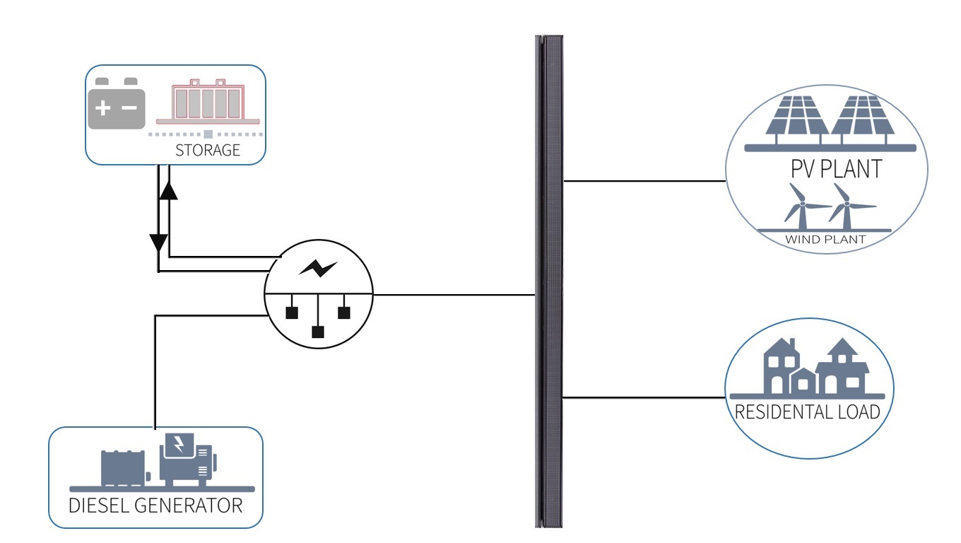
Figure 1: The figure above shows an example of microgrid topology that contains all the elements in our model. The network is arranged as follows: photovoltaic panels and wind turbines provide renewable generation, a diesel generator provides dispatchable power for the village and a battery storage system is used to inject or withdraw energy.

2.1 Residual Demand

Consider two stochastic processes $L_{t}$ and $R_{t}$, the former represents the demand/load and the latter the production through the renewable generators. Notice that both processes are uncontrolled and they represent, respectively, the unconditional withdrawal or injection of power in the system (constant during time step). For the purpose of managing the microgrid, the controller is interested only in the net effect of the two processes denoted by the process $X_{t}$:

$$X_{t}=L_{t}-R_{t}\;;\quad t\in\{0,\,1,\,\dots,\,T\}.$$ (1)

Remark 2.

The state variable $X_{t}$ represents the residual demand of power at each time $t$, such that for $X_{t}>0$, we should provide power through the battery or diesel generator and for $X_{t}<0$ we can store the extra power in the battery.

For simplicity, we model the residual demand as an AR(1) process, the discrete equivalent of an Ornstein–Uhlenbeck process. In practical applications we expect $X_{t}$ to be an $\mathbb{R}$-valued mean reverting process with many different sources of noise and time dependent random parameters; our formulation avoids the cumbersome notation using constants in place of stochastic processes still providing scope for generalization. The process $X_{t}$ is driven by the following difference equation, starting from an initial point $X_{0}=x_{0}$:

$$X_{t+1}=X_{t}+b(\Lambda_{t}-X_{t})\Delta t+\sigma\sqrt{\Delta t}\;\xi_{t}\;;\quad t\in\{0,1,\dots,T\}$$ (2)

where $\xi_{t}\sim\mathcal{N}(0,1)$, $\Delta t$ is the amount of time before new information is acquired, $b$ is the mean reversion speed, $\sigma$ the volatility of the process and $\Lambda_{t}$ is the time dependent mean reversion level.

Remark 3.

In real applications the function $\Lambda_{t}$ should represent the best forecast available for future residual demand at the time of the estimation of the policy.

2.2 Diesel generator

The Diesel generator represents the controlled dispatchable unit. The state of the generator is represented by $m_{t}=\{0,1\}$. If $m_{t}=0$ then the diesel generator is OFF, while it is ON when $m_{t}=1$. When the engine is ON, it produces a power output denoted by $d_{t}\in[d_{min},d_{max}]$ at time $t$, for $d_{min}>0$.

Notice that, in addition, when the engine is turned ON, an extra amount of fuel is burned in order for the generator to warm up and reach working regime. We model the cost of burning extra fuel with a switching cost $\mathcal{K}$ that is paid every time the switch changes from $0$ to $1$. The fuel consumption of the diesel generator is modeled by an increasing function $\rho(d_{t})$ which maps the power $d_{t}$ produced during one time step into the quantity of diesel necessary for such output. Denoting by $P_{t}$ the price of fuel at time $t$, the cost of producing $d_{t}$ KW of power at one time step is $P_{t}\rho(d_{t})$; for simplicity we take a constant price of the fuel $P_{t}=p$. Two examples of efficiency functions $\rho$ are described in figure 2.

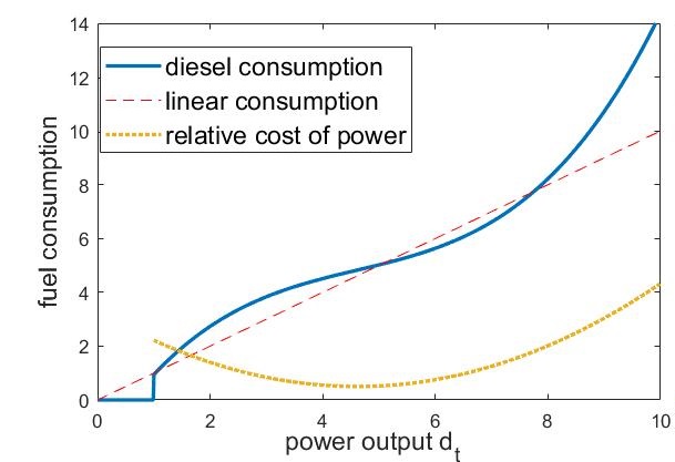
(a) $\rho(d)=\frac{(d-6)^{3}+6^{3}+d}{10}$

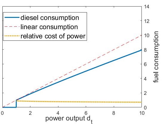
(b) $\rho(d)=d^{0.9}$

Figure 2: The panels above show two examples of efficiency function (litres/KW), on the left $\rho(d)=\frac{(d-6)^{3}+6^{3}+d}{10}$, typical of a generator designed to operate at medium regime, on the right $\rho(d)=d^{0.9}$, typical of a generator designed to operate a full capacity.

2.3 Dynamics of the Battery

The storage device is directly connected to the microgrid and therefore its output is equal to the imbalance between demand $X_{t}$ and diesel generator output $d_{t}$, when this is allowed by the physical constraint. The battery therefore is discharged in case of insufficiency of the diesel output and charged when the diesel generator and renewables provide a surplus of power.

Let us denote the power output of the battery by $B^{d}_{t}$ and its power rating by $B^{\max}$ and $B^{\min}$, where $B^{\max}$ and $B^{\min}$ represent respectively the maximum and minimum output. Thus:

$$B^{d}_{t}=\frac{I_{t}^{d}-I_{\max}}{\Delta t}\vee\big{(}B^{\min}\vee(X_{t}-d_{t})\wedge B^{\max}\big{)}\wedge\frac{I_{t}^{d}}{\Delta t}$$ (3)

The case where $B^{d}_{t}<0$, represents that the battery is charging while the case where $B^{d}_{t}>0$, represents that the battery is supplying power.

Notice then that an energy storage has a limited amount of capacity after which it can not be charged further, as well as an “empty” level below which no more power can be provided from the battery. We denote the state of charge by the controlled process $I^{d}_{t}$ which is described by the following equation:

$$I^{d}_{t+1}=I^{d}_{t}-B^{d}_{t}\Delta t,\quad t\in\{0,1,\dots,T-1\},\quad I^{d}_{0}=w_{0}$$ (4)

here $I^{d}_{t}\in[0,I_{max}]$ and $B^{d}_{t}\in[B^{\min},B^{\max}]$, for $B^{\min}<0$ and $B^{\max}>0$. For simplicity we assume that the battery is $100\%$ efficient. Notice that we used superscript $d$ on $B^{d}$ and $I^{d}$ to highlight the dependence of these processes on the controlled diesel output $d_{t}$.

Intuition tells us that the bigger the battery, the less diesel will be needed to run the operations of the microgrid. This is true because a bigger battery would allow to store for later use a bigger proportion of the excess power produced by the renewables. Batteries however are very expensive, and the cost per KWh of capacity scales almost linearly for the kind of devices we consider in this paper (parallel connection of smaller batteries), hence it is important to find the optimal size of battery for the needs of each specific microgrid.

2.4 Management of the Microgrid

The purpose of the microgrid is to provide a cheap and reliable source of power supply to at least match the demand. Therefore, we search for a control policy for the diesel generator which minimizes the operating cost and produces enough electricity to match the residual demand. In order to assess how well we are doing in supplying electricity, we introduce the controlled imbalance process $S_{t}$ defined as follows:

$$S_{t}=X_{t}-B^{d}_{t}-d_{t}\quad t\in[0,T]$$ (5)

Ideally, the owner of the Microgrid would like to have $S_{t}=0\quad\forall\;t$. This situation represents the perfect balance of demand and generation. When $S_{t}>0$ we observe a blackout, residual demand is greater than the production meaning that some loads are automatically disconnected from the system. The situation $S_{t}<0$ is defined as a curtailment of renewable resources and takes place when we have a surplus of electricity.

We treat the two scenarios, blackout and curtailment asymmetrically. To ensure no-blackout $S_{t}\leq 0$ and regular supply of power, we impose a constraint on the set of admissible controls:

$$\begin{split}&S_{t}\leq 0\\ \text{i.e. }&d_{t}\geq X_{t}-B^{d}_{t}.\end{split}$$ (6)

However, for $S_{t}<0$ i.e. surplus of electricity, we penalize the microgrid using a proportional cost denoted by $C$. Large penalty would lead to low level of curtailment and can be thought of as a parameter in the subsequent optimization problem.

A rigorous mathematical description of the microgrid management problem follows in section 3.

3 Stochastic optimization problem

We state now the stochastic control problem for the diesel generator operating in a microgrid system as described in section 2. In practice we seek a control that minimizes the cost of diesel usage $p\rho(d)$, the switching cost $\mathcal{K}$ and the curtailment cost $C|S_{t}|\mathds{1}_{\{S_{t}<0\}}$, under the no black-out constraint $S_{t}\leq 0$.

Note that, given the type of control we have on the diesel generator, we can frame the optimization problem as a special case of stochastic control problems known as optimal switching problems.

Let us denote by $\mathcal{F}_{t}$ the filtration generated by the residual demand process $(X_{s})_{s=0}^{t}$, the state of charge process $(I_{s}^{d})_{s=0}^{t}$ and the current regime $m_{t}$, which represents all the information available on the system up to time $t$. In practice, given the markovianity of the problem, we have that $\mathcal{F}_{t}$ is reduced to the $\sigma$-field generated by the triple $(X_{t},I_{t}^{d},m_{t})$.

Let us define the pathwise value $\mathcal{J}$, given by

$$\mathcal{J}(t,\textbf{X}_{t},\textbf{I}_{t},m_{t};d_{t})=\sum_{s=t}^{T-1}\mathds{1}_{\{m_{s+1}-m_{s}=1\}}\mathcal{K}+p\rho(d_{s})+C|S_{s}|\mathds{1}_{\{S_{s}<0\}}+g(I^{d}_{T}).$$ (7)

where $(\textbf{X}_{t},\textbf{I}_{t},m_{t};d_{t})=(X_{s},I^{d}_{s},m_{s};d_{s})_{s=t}^{T}$. As a consequence, we define the value function as:

$$V(t,x,w,m)=\min_{d_{t}=(d_{u})_{u=t}^{T}}\left\{\mathbb{E}\left[\mathcal{J}(t,\textbf{X}_{t},\textbf{I}^{d}_{t},m_{t};d_{t})\Big{|}X_{t}=x,I^{d}_{t}=w,m_{t}=m\right]\right\}$$ (8)

subject to $$d_{t}\geq X_{t}-B^{d}_{t}\quad\;\forall t$$ (9a)

$$d_{t}\in[d_{min},d_{max}]\cup\{0\}.$$ (9b)

$$B^{d}_{t}=\frac{I_{t}^{d}-I_{\max}}{\Delta t}\vee\big{(}B^{\min}\vee(X_{t}-d_{t})\wedge B^{\max}\big{)}\wedge\frac{I_{t}^{d}}{\Delta t}$$ (9c)

where (9a) represents the black-out constraints translated for the power produced by the diesel generator, (9b) represents the minimum and maximum power output of the generator and (9c) models the physical constraints of the battery: maximum input/output power and maximum capacity.

From equation (8), we can write the associated dynamic programming formulation which helps understand the structure of the problem composed of two optimal control problems: an optimal switching problem between being in the regime ON or OFF, and another absolutely continuous control problem assuming the regime is ON. The equation reads as follows:

$$V(t,x,w,m)=\underset{d\in\mathcal{U}_{t}}{\min}\Big{(}\mathds{1}_{\{m_{t+1}-m_{t}=1\}}\mathcal{K}+p\rho(d)+C|S_{t}|\mathds{1}_{\{S_{t}<0\}}+\mathcal{C}(t,x,w,m;d)\Big{)},$$ (10)

where

$$\mathcal{C}(t,x,w,m;d)=\mathbb{E}[V(t+1,X_{t+1},I_{t+1},m_{t+1})|X_{t}=x,I_{t}=w,d_{t}=d,m_{t}=m],$$

is the conditional expectation of the future costs and $\mathcal{U}_{t}$ is the collection of admissible controls $d$ at each time step $t$, i.e.

$$\mathcal{U}_{t}:=\{d_{t}:\text{equations \eqref{cond_st} - \eqref{cond_bat} are satisfied and $d_{t}$ adapted to }\mathcal{F}_{t}\}.$$ (11)

In order to ensure that the set of admissible controls is nonempty we introduce the following assumption:

Assumption 1.

The diesel generator is powerful enough to supply demand at all times, i.e there is always a control $d$ that satisfies the blackout constraint.

Remark 4.

We enforce assumption 1 by redefining the residual demand process with a truncated version of (1), such that $\tilde{X}_{t}=\min(X_{t},X_{\max})$ is the residual demand. In practice this is reasonable because the maximum power that could be required from the microgrid is known apriori and the diesel generator is generally sized to the maximum capacity installed on the system. For the sake of notational simplicity, we will drop the $\sim$ on the variable $\tilde{X}_{t}$ from the following sections.

Note that (10) provides a direct technique to solve problem (8), iterating backward in time from a known terminal condition and solving a static, one period, optimization problem at each time step. The only difficulty in this procedure lies in the estimation of conditional expectations of future value function, which can not be computed exactly. In the next section 4 we will focus on the numerical solution of (8).

4 Numerical Resolution

In this section we describe the algorithm which we want to employ in the solution of the energy management problem for the Microgrid system described in section 3. The main mathematical difficulty comes from the approximation of conditional expectations in (10), which we will tackle using a family of methods called Regression Monte Carlo.

The algorithm we propose fully exploits the dynamic programming formulation (10): we start generating a set of simulations (scenarios) of the process $X$, which we will refer to as training points, then we optimize our policy so that it performs well, on average (weighted on the probability of each scenario), on the different scenarios.

In practice, we initialize the value function at last time step in the backward procedure to be equal to the terminal condition $g$. We then iterate backward in time and at each time step over each training point we choose the control that minimizes the sum of one step cost function and the estimated conditional expectation of the future costs $\tilde{\mathcal{C}}(t,x,w,m;d)$. Note that, as expected, the conditional expectation is a function of time, the state of the system $(x,w)$ and the state of the diesel generator, represented by the ON/OFF switch $m$ and the control $d$.

As the iteration reaches the initial time point we collect a set of optimal actions for each time step and many different scenarios; in addition, since the problem is Markovian, we can summarize such strategies in the form of control maps: best action at each time $t$ given a pair of state variables $(X_{t},I_{t})$ and state of the diesel generator $m_{t}$. We propose three different techniques to compute $\tilde{\mathcal{C}}$ in section 4.1.

A fair assessment of the quality of the control policies approximated by the algorithm just introduced is obtained by running a number of forward Monte Carlo simulations of the residual demand, controlling the system using such policies and then taking the average performance.

We give a general description of the pseudo code in algorithm 1.

Remark 5.

Notice that it is typical of Regression Monte Carlo algorithms to provide the optimal policy only implicitly, in the form of minimizer of an explicit parameterized function. The outputs of the algorithm are therefore the parameters (regression coefficients) of such function.

Algorithm 1 Regression Monte Carlo algorithm for Microgrid management

input: number of basis $K$, number of training points $M$, discretisation of the inventory $D$, time-steps $N$.

1:optimization:

2:if Inventory discretisation then

3:     Generate a customary grid $\{w_{0},\ldots,w_{D}\}$ points over the domain of $I_{t}$.

4:     Simulate $\{X_{t}^{j}\}_{j,t=1}^{M^{\prime},N}$ according to its dynamics where $M^{\prime}=M/(D+1)$;

5:     Define $\{X_{t}^{j},I_{t}^{j}\}_{j=1}^{M}$ as cross product of $\{X_{t}^{j}\}_{j=1}^{M^{\prime}}$ and $\{w_{j}\}_{j=0}^{D}$ for $\forall t$

6:if Regression 2D then

7:     if Regress Later then

8:         Generate $\{X_{t}^{j},I_{t}^{j}\}_{j,t=1}^{M,N}$ accordingly to a distribution $\mu$;      

9:     if Regress Now then

10:         Generate $\{X_{t}^{j}\}_{j,t=1}^{M,N}$ according to its dynamics and $\{I_{t}^{j}\}_{j,t=1}^{M,N}$ according to a distribution $\mu$;      

11:Initialize the value function $V(N,X_{N}^{j},I_{N}^{j},1)=V(N,X_{N}^{j},I_{N}^{j},0)=g(I_{N}^{j}),\quad\forall j=1,\,\dots,\,M$;

12:for $t=N$ to $1$ do

13:     Compute the approximated continuation value $\tilde{\mathcal{C}}$ using Algorithms 3 or 2

14:     for $j=1$ to $M$ do

15:         for $m=0$ to $1$ do

16:              $F=\tilde{\mathcal{C}}(X_{t}^{j},I_{t}^{j};0,0)$

17:              

$$V(t,X_{t}^{j},I_{t}^{j},m)=\begin{cases}\Big{(}\min\limits_{d\in\mathcal{U}_{t}\setminus\{0\}}\Big{\{}p\rho(d)+C|S_{t}|\mathds{1}_{\{S_{t}<0\}}+\tilde{\mathcal{C}}(X_{t}^{j},I_{t}^{j};1,d)\Big{\}}+\mathcal{K}\mathds{1}_{\{m=0\}}\Big{)}\wedge F&\quad\text{if }0\in\mathcal{U}_{t}\\ \min\limits_{d\in\mathcal{U}_{t}}\Big{\{}p\rho(d)+C|S_{t}|\mathds{1}_{\{S_{t}<0\}}+\tilde{\mathcal{C}}(X_{t}^{j},I_{t}^{j};1,d)\Big{\}}+\mathcal{K}\mathds{1}_{\{m=0\}}&\quad\text{otherwise}\end{cases}$$

              

18:simulation:

19:initialize processes

20:for $t=1$ to $N-1$ do

21:     for $j=1$ to $M$ do

22:         $F_{1}=\tilde{\mathcal{C}}(X_{t}^{j},I_{t}^{j};0,0)$

23:         $F_{2}=\min\limits_{d\in\mathcal{U}_{t}\setminus\{0\}}\Big{\{}p\rho(d)+C|S_{t}|\mathds{1}_{\{S_{t}<0\}}+\tilde{\mathcal{C}}(X_{t}^{j},I_{t}^{j};1,d)\Big{\}}+\mathcal{K}\mathds{1}_{\{m_{t}^{j}=0\}}$

24:         $m_{t+1}^{j}=\mathds{1}_{\{(0\notin\mathcal{U}_{t})\text{ or }(0\in\mathcal{U}_{t}\text{ and }F_{2}<F_{1})\}}$

25:         if $m_{t+1}^{j}=1$ then

26:              $d_{t}=\mathop{\rm argmin}\limits_{d\in\mathcal{U}_{t}}\Big{\{}p\rho(d)+C|S_{t}|\mathds{1}_{\{S_{t}<0\}}+\tilde{\mathcal{C}}(X_{t}^{j},I_{t}^{j};1,d)\Big{\}}$          

27:         compute $X_{t+1}^{j}$ and $I_{t+1}^{j}=I_{t}^{j}-B^{d}_{t}\Delta t$

28:         $J_{t+1}^{j}=J_{t}^{j}+p\rho(d_{t})+C|S_{t}|\mathds{1}_{\{S_{t}<0\}}+\mathcal{K}\mathds{1}_{\{m_{t+1}-m_{t}=1\}}$      

29:$V(0,x,w,m)=\frac{1}{M}\sum_{j=1}^{M}(J_{N}^{j}+g(I_{N}^{j}))$

output: control policy $\{d_{t}\}$, value function $V$.

4.1 Regression for continuation value

In this section we present the numerical techniques we use to estimate conditional expectations $\mathcal{C}(t,x,w,m;d)$ in algorithm 1. These techniques belong to the realm of Regression Monte Carlo methods, and in particular these specifications allow to deal with degenerate controlled processes (the inventory). We focus on two main variants: a two dimensional approximation of the conditional expectation and a discretisation technique which considers a collection of one dimensional approximations.

In particular, we test three algorithms: Grid Discretisation, Regress Now and Regress Later. Grid Discretization is characterized by a one dimensional projection in the residual demand dimension repeated at different inventory points. Regress Now/Later, on the other hand, use a two dimensional regression in residual demand and inventory. Moreover, while Grid Discretization and Regress Now require projection of the value function at $t+1$ on $\mathcal{F}_{t}$ measurable basis functions, Regress Later requires an $\mathcal{F}_{t+1}$ projection. For details on these techniques see balata17 for regress later,boogert08; warin for GD and ludkovski10 for 2D regress now. Note that in the three algorithms we repeat the regression approximation for both values of $m$. An open source platform has also been developed to numerically solve wide variety of stochastic optimization problems in StOpt.

Let us denote by $\{X_{t}^{j}\}_{j=1}^{M}$ the collection of training points at time $t$, similar notation is used for the inventory $\{I_{t}^{j}\}_{j=1}^{M}$.

4.1.1 Grid Discretisation

Grid discretisation is characterized by a one dimensional approximation of the conditional expectation repeated at different levels of inventory. Let $\Upsilon_{I}=\{w_{0}=0,\dots,w_{D}=I_{max}\}$ be a discretisation of the state space of the inventory and $\{X_{t}^{j}\}_{j=1,t=1}^{M,N}$ be generated from a forward simulation of the dynamics of $X$. We define the approximation of the continuation value on the grid $\Upsilon_{I}$ by regressing the set of value functions $\{V(t+1,X_{t+1}^{j},w_{i})\}_{j=1}^{M}$ over the basis functions $\{\phi_{k}(x)\}_{k=1}^{K}$ for each $\{w_{i}\}_{i=0}^{D}$, obtaining:

$$\hat{\mathcal{C}}(t,x,w_{i};m)=\sum_{k=1}^{K}\alpha_{k,i,m}^{t}\phi_{k}(x)\,,\quad i=0,\,1,\,\dots,\,D,$$

where we compute a collection of regression coefficients through least square minimization

$$\bm{\alpha}^{t}_{i,m}=\mathop{\rm argmin}\limits_{a\in\mathbb{R}^{K}}\Big{\{}\frac{1}{M}\sum_{j=1}^{M}\big{(}V(t+1,X_{t+1}^{j},w_{i},m)-\sum_{k=1}^{K}a_{k}\phi(X_{t}^{j})\big{)}^{2}\Big{\}},$$

where we define $\mathbb{R}^{K}\ni\bm{\alpha}^{t}_{i,m}=(\alpha^{t}_{1,i,m},\,\dots,\,\alpha^{t}_{K,i,m})$.

Note that the least square projection is a sample estimation of the $L^{2}$ projection induced by the conditional expectation, for this reason we can approximate the function $\mathcal{C}(t,\cdot)$ using a least square projection of the value function at time $t+1$. However, as we have not included the inventory in the basis functions, we need to interpolate between values of $\hat{\mathcal{C}}(t,x,w_{i};m)$ in order to obtain an estimation of the value function for $I_{t}\in(w_{i},w_{i+1})$. Let us define by $\tilde{\mathcal{C}}(t,x,w;m,d)$ the linear interpolation

$$\tilde{\mathcal{C}}(t,x,w;m,d)=\omega(t,w,d)\hat{\mathcal{C}}(t,x,w_{i},m)+\big{(}1-\omega(t,w,d)\big{)}\hat{\mathcal{C}}(t,x,w_{i+1},m)\,,\quad w-B_{t}^{d}\Delta t\in[w_{i},w_{i+1}),$$

where $\omega(t,w,d)=\frac{w_{i+1}-w+B_{t}^{d}\Delta t}{w_{i+1}-w_{i}}$ and $i=0,\,\dots,\,D$.
Details of the algorithms are given in the pseudocode 2.

Algorithm 2 Regression technique for continuation value: Grid Discretisation

input: $\{V(t+1,X_{t+1}^{j},I_{t+1}^{j},m)\}_{j=1}^{M}$, $\{\phi_{k}\}_{k=1}^{K}$.

1:for $i=0$ to $D$ do

2:     $\bm{\alpha}^{t}_{m}=\mathop{\rm argmin}\limits_{a}\Big{\{}\sum\limits_{j=1}^{M}\Big{(}V(t+1,X_{t+1}^{j},w_{i},m)-\sum\limits_{k=1}^{K}a_{k}\phi_{k}(X^{j}_{t})\Big{)}^{2}\Big{\}}$;

3:     Define $\hat{\mathcal{C}}(t,x,w_{i},m)=\sum_{k=1}^{K}\alpha^{t}_{k,i,m}\phi_{k}(x)$, $m=0,1$;

4:Define $\tilde{\mathcal{C}}(t,x,w;m,d)=\frac{w_{i+1}-w+B_{t}^{d}\Delta t}{w_{i+1}-w_{i}}\hat{\mathcal{C}}(t,x,w_{i};m,d)+\frac{w-B_{t}^{d}-w_{i}}{w_{i+1}-w_{i}}\hat{\mathcal{C}}(t,x,w_{i+1};m,d)$, $w\in[w_{i},w_{i+1})$, $m=0,1$.

output: $\tilde{\mathcal{C}}$, $\{\alpha^{t}_{k,i,m}\}_{k=1,i=1,m=0}^{K,D,1}$.

4.1.2 2D Regression

Contrary to the grid discretisation approach, the 2D regression methods approximate the conditional expectation of the value function as a surface, function of both residual demand $X$ and inventory $I$, without the need for interpolation. In the problem we consider, the control only acts on a degenerate (deterministic) process and we can therefore test two specifications of the method: “Regress Now”, where we project over $\{\phi_{k}(X_{t},I_{t+1})\}_{k=1}^{K}$ and “Regress Later”, where we project over $\{\phi_{k}(X_{t+1},I_{t+1})\}_{k=1}^{K}$. The terminology Regress Now or Regress Later is attributed to the time step of the exogenous variable $X_{t}$ used in the projection.

In Regress Now, we generate training points $\{X_{t}^{j}\}_{j=1,t=1}^{M,N}$ from a forward simulation of the dynamics of $X$ and $\{I_{t}^{j}\}_{j=1,t=1}^{M,N}$ from a distribution $\mu_{N}$ on $[0,I_{max}]$. In Regress Later, on the other hand, we generate both processes $\{X_{t}^{j},I_{t}^{j}\}_{j=1,t=1}^{M,N}$ from an appropriate distribution $\mu_{L}$, for details see balata17. In the following we will generalize the discussion of the two approaches by using the subscript $r$ with realization $t$ to indicate Regress Now algorithm and $t+1$ to indicate Regress Later. As training measures we choose $\mu_{N}$ to be the Lebesgue measure on $[0,I_{\max}]$ and $\mu_{L}$ to be Lesbegue measure on $[0,I_{\max}]\times[-X_{\max},X_{\max}]$.

The regression coefficients in the 2D regression Monte Carlo method are computed by least-square projection as:

$$\bm{\alpha}^{t}_{m}=\mathop{\rm argmin}\limits_{a\in\mathbb{R}^{K}}\Big{\{}\frac{1}{M}\sum_{j=1}^{M}\big{(}V(t+1,X_{t+1}^{j},I_{t+1}^{j},m)-\sum_{k=1}^{K}a_{k}\phi(X_{r}^{j},I_{t+1}^{j})\big{)}^{2}\Big{\}},$$

where we define $\mathbb{R}^{K}\ni\bm{\alpha}^{t}_{m}=(\alpha^{t}_{1,m},\,\dots,\,\alpha^{t}_{K,m})$.

Let us recall, denoting by $\bm{\phi}$ the vector $\big{(}\phi_{1}(\cdot),\,\dots,\,\phi_{K}(\cdot)\big{)}$, that the coefficients $\bm{\alpha}^{t}_{m}$ can be computed explicitly by

$$\bm{\alpha}^{t}_{m}=\Big{(}\mathbb{E}_{\mu}\big{[}\bm{\phi}\bm{\phi}^{T}\big{]}\Big{)}^{-1}\mathbb{E}_{\mu}\Big{[}V(t+1,X_{t+1},I_{t+1},m)\bm{\phi}\Big{]}^{T}\approx\Big{(}\sum_{j=1}^{M}\bm{\phi}\bm{\phi}^{T}\Big{)}^{-1}\sum_{j=1}^{M}V(t+1,X_{t+1}^{j},I_{t+1}^{j},m)\bm{\phi}^{T}$$

and therefore, even though the regression coefficients are random (sample average approximation of expectations with respect to the measure $\mu$) they are independent of $\mathcal{F}_{t}$. Given the previous remark we can estimate the conditional expectation of future value through:

$$\tilde{\mathcal{C}}(t,x,w;m,d)=\mathbb{E}\Big{[}\sum_{k=1}^{K}\alpha_{k,m}^{t}\phi_{k}(X_{r},I_{t+1})\Big{|}\mathcal{F}_{t}\Big{]}=\sum_{k=1}^{K}\alpha_{k,m}^{t}\mathbb{E}\Big{[}\phi_{k}(X_{r},I_{t+1})\Big{|}X_{t}=x,\,I_{t}=w,\,d_{t}=d\Big{]}.$$

The explicit value of $\mathbb{E}\Big{[}\phi_{k}(X_{r},I_{t+1})\Big{|}X_{t}=x,\,I_{t}=w,\,d_{t}=d\Big{]}$ now depends on $r$, i.e. whether we are using “Regress Now” or “Regress Later” to deal with the uncontrolled residual demand. In the first case we simply obtain, from the measurability of $X_{t}$,

$$\mathbb{E}\Big{[}\phi_{k}(X_{t},I_{t+1})\Big{|}\mathcal{F}_{t}\Big{]}=\phi_{k}(x,w-B^{d}_{t}\Delta t)=:\tilde{\phi}_{k}(x,w,d).$$

In the second case we need to compute the expectation with respect to the randomness contained in the transition function from $X_{t}$ to $X_{t+1}$ and we simply write

$$\mathbb{E}\Big{[}\phi_{k}(X_{t+1},I_{t+1})\Big{|}\mathcal{F}_{t}\Big{]}=\mathbb{E}_{\xi}\Big{[}\phi_{k}(x+b(\Lambda_{t}-x)\Delta t+\sigma\sqrt{\Delta t}\xi,w-B^{d}_{t}\Delta t)\Big{]}=:\hat{\phi}_{k}(x,w,d).$$

Remark 6.

For polynomial basis functions, i.e. $\phi_{k}(X_{t+1},I_{t+1}):=X^{p}_{t+1}I^{q}_{t+1}$, the conditional expectation $\hat{\phi}_{k}(x,w,d)$ can be written in closed form as:

$$\begin{split}\hat{\phi}_{k}(x,w,d)&=\mathbb{E}\big{[}X^{p}_{t+1},I^{q}_{t+1}\big{|}X_{t}=x,I_{t}=w,d_{t}=d\big{]}\\ &=I_{t+1}^{q}\sigma^{p}dt^{\frac{p}{2}}\sum_{k=0}^{p}\mathbb{I}_{\{(p-k)\text{ is odd}\}}{p\choose k}\Big{(}x\frac{1-\lambda dt}{\sigma\sqrt{dt}}\Big{)}^{k}\prod_{j=1}^{\frac{p-k}{2}}(2j-1)\end{split}$$

Using the notation just introduced we can summarize the differences between the two techniques in the following table:

	$\phi_{k}$	$\mathbb{E}[\phi_{k}|X_{t},I_{t},d_{t}]$	$\mathcal{C}(t,x,w,m;d)$
RN	$(X_{t},I_{t+1})$	$\phi_{k}(X_{t},I_{t}-B^{d}_{t}\Delta t)$	$\sum_{k=1}^{K}\alpha_{k,m}^{t}\tilde{\phi}_{k}(x,w,d)$
RL	$(X_{t+1},I_{t+1})$	$\mathbb{E}[\phi_{k}(X_{t}+b(\Lambda_{t}-X_{t})\Delta t+\sigma\sqrt{\Delta t}\xi,I_{t}-B^{d}_{t}\Delta t)]$	$\sum_{k=1}^{K}\alpha_{k,m}^{t}\hat{\phi}_{k}(x,w,d)$

Details of the algorithms are given in the pseudocode 3 .

Algorithm 3 Regression technique for continuation value: 2D Regression

input: $\{V(t+1,X_{t+1}^{j},I_{t+1}^{j},m)\}_{j=1}^{M}$, $\{\phi_{k}\}_{k=1}^{K}$.

1:if Regress Later then

2:     $r=t+1$

3:else if Regress Now then

4:     $r=t$

5:$\bm{\alpha}^{t}_{m}=\mathop{\rm argmin}\limits_{a}\Big{\{}\sum\limits_{j=1}^{M}\Big{(}V(t+1,X_{r}^{j},I_{t+1}^{j},m)-\sum\limits_{k=1}^{K}a_{k}\phi_{k}(X^{j}_{r},I^{j}_{t+1})\Big{)}^{2}\Big{\}}$, $m=0,1$;

6:Define $\tilde{\mathcal{C}}(t,x,w;m,d)=\sum_{k=1}^{K}\alpha^{t}_{k,m}\mathbb{E}[\phi_{k}(X_{r},I_{t+1})|x,w,d]$

output: $\tilde{\mathcal{C}}$, $\{\alpha^{t}_{k,m}\}_{k=1,m=0}^{K,1}$.

5 Numerical Experiments

In this section we use the algorithms introduced in section 4 to solve a simple instance of the microgrid management problem. We fix some base parameters and test the three algorithms; the one performing best is then used to study the sensitivity of the control policy and of the operational costs on changes in system parameters, hoping to gain some insight on the optimal design of the microgrid.

We now list the base parameters chosen for the numerical experiments; notice that the "s" column indicates whether a sensitivity analysis is run for such parameter. For the meaning of the parameters refer to section 2.

parameter	value	s
$T$	$100h$
$\Delta t$	$0.25h$
$b$	$0.5$	*
$\sigma$	$2$	*
$\Lambda_{t}$	$0,\,\forall t$

parameter	value	s
$I_{max}$	$10$ KWh	*
$\rho(d)$	$\frac{(d-d^{*})^{3}+(d^{*})^{3}+d}{10}\frac{litre}{\text{KW}}$
$d^{*}$	$6$ KW
$p$	$1$ €
$g(i)$	$0,\,\forall i$

parameter	value	s
$d_{min}$	$1$KW
$d_{max}$	$10$KW
$K$	$5$ €	*
$C$	$0$ €	*

According to the parameters table above, and recalling remark 4 the residual demand has the following dynamics:

$$X_{t+1}=\big{(}X_{t}(1-0.5\Delta t)+\sigma\sqrt{\Delta t}\xi_{t}\big{)}\wedge 10,\quad t\in\{0,1,\dots,T-1\},$$ (12)

where $\xi_{t}\sim\mathcal{N}(0,1)$.

We decided to use such simple dynamics for illustrative purposes in order to make the sensitivity of the optimal control policy to the remaining parameters more straight forward to understand.

Consider now that for the parameters listed above, the problem is time homogeneous. We have also observed empirically that the estimated continuation values tend to forget the terminal condition rather quickly. We show in Figure 3 that the regression coefficients for all algorithms converge to a stationary value time steps, suggesting that optimization ran for longer time horizons would not bring any noticeable effect to control policy. Since all three methods use polynomial basis of degree two for the projection, it also allows for easy comparison of the dynamics of the coefficients across methods. For example, at inventory level $I=0$ the dynamics of the coefficient for $x$ achieves same stationary level for both Grid Discretization and Regress Now. Although an exact comparison is not possible between Regress Now and Regress Later, we continue to observe similar sign and dynamics for each of the coefficients. However, getting away with almost no noise in the dynamics of the estimated coefficients of Regress Later compared to Regress Now is essentially magical.

As a result, we define a stationary policy $d(x,w,m)$ to be used in a longer time horizon than the one employed for its estimation which performance are comparable to the time dependent policy $d(t,x,w,m)$.

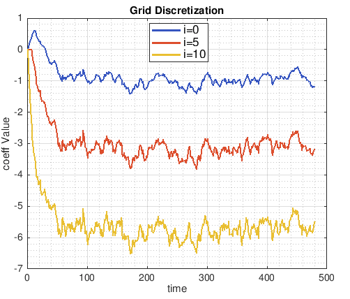
(a)

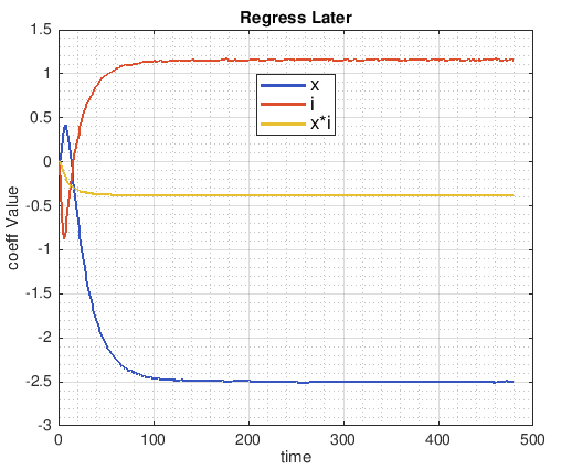
(b)

(c)

Figure 3: In the three panels above we display the estimated regression coefficients corresponding to the basis $\{x,i,x\,i\}$ in the case of 2D regression, and $\{x\}$ at three different inventory levels for GD for $m_{t}=1$. Although we used basis function up to polynomial degree 2, we present few coefficients for clarity of presentation. Notice that the time axis is inverted to show the number of time steps computed backward. Remarkable smooth coefficients are computed by the Regress Later algorithm.

We finally tested the value of both stationary and time dependent policy and found that the performance of the stationary policy is comparable to that of the time dependent policy.

5.1 Analysis of the controllers

In this section we compare the control policies estimated by the three algorithms and we try to assess whether one of the approaches is preferable.

5.1.1 Control maps

We compare now the stationary control policies produced by the different algorithms; recall that these policies are feedback to the state, i.e. can be written as function $d_{m}(x,w)$. Figure 4 displays an example of the feedback control policy in the form of control map, a graphical representation of the value of the optimal control for each pair $(x,w)$.

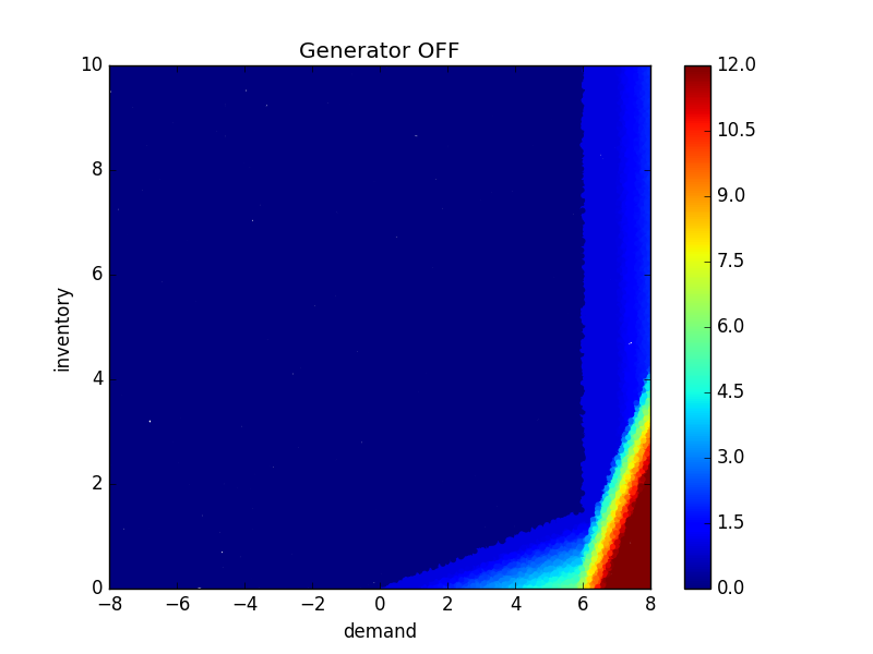
(a)

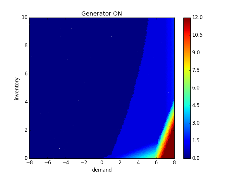
(b)

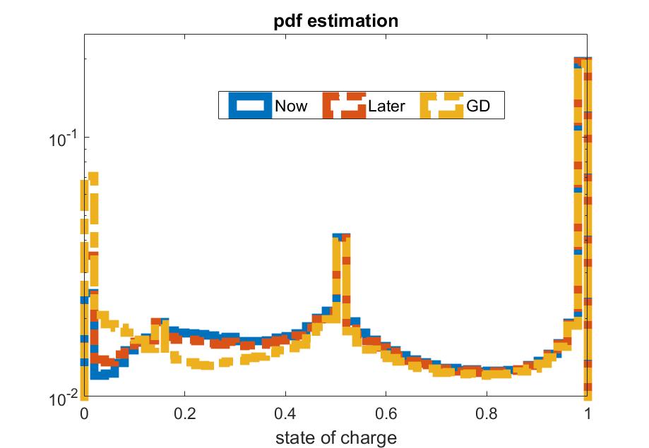
(c)

Figure 4: In the figure above we show, in the two left-most panels, an example of control map produced by the Regress Later algorithm. Notice the difference depending on the state of the generator. In the right-most panel we display the estimated probability density function of the state of charge of the battery associated with the use of the three policies. It can be observed that Regress Later and Grid discretization induce very similar distributions.

We observed that the three policies agree with the intuition that the diesel generator should produce more power when residual demand is high and inventory is low. We can also notice that the switching cost influences the policy, forcing the diesel to keep running for longer in order to charge the battery sufficiently and avoid turning ON and OFF the generator too often. Just by observation of the control maps little difference can be found among the algorithms, we display in Figure 4 the effect of the control policy on a the state of charge of the battery. It can be observed from the estimated unconditional probability density of the process $I$ that the policies induced by Regress Now and Regress Later are very similar. Both seem to induce a peculiar mass of probability around $I_{n}=2.5$, differentiating the behavior of the inventory compared to Grid Discretization. The distribution of the state of charge, obtained by plotting the histogram of all simulations over all time steps, shows that Regress Now and Regress Later does not fully exploit the whole inventory but rather they are more conservative, saving energy to avoid to turn ON the diesel generator in the future. In the next section we will investigate the value associated to this control maps.

5.1.2 Performance of the policies

In order to assess the performance of each policy in an unbiased manner, we select a collection of simulated paths of the residual demand process $X$, and record the costs associated with managing the microgrid as indicated by each control map.

We first study how the quality of each policy improves when we increase the computational budget given to each algorithm to compute the stationary policy. In Figure 5, we show the estimated value of the policy when the initial state of the system is $(x,i,m)=(0,5,0)$ for polynomial basis functions of increasing degree, for 2D regression. In case of GD we increase the number of discretisation points for the inventory. In particular we make the computational time increase by providing the problem with more training points and more parameters to use in the definition of $\mathcal{C}$ as increasing the number of basis functions. In the case of 2D regression, surprisingly, we noticed that the performance of the estimated control improves only when polynomials of even degree are added, and the effect is more prominent for Regress Later.

We notice from the comparison that Grid Discretisation converges quickly, resulting in the best algorithm in terms of trade off between running time and precision. Among the 2D regressions, we observe similar bias for Regress Now and Regress Later (not displayed in order to maintain clear presentation, but available on request), however latter has lower standard error. This is not surprising because Regress Later has only one element of approximation error due to finite basis functions while Regress Now has error attributed to two sources, first, due to finite basis function and second, pathwise estimation of the conditional expectation.

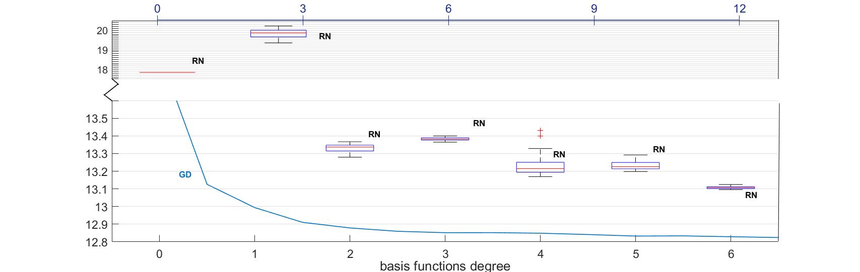
Figure 5: The figure in display shows the reduction in operating cost when higher degree polynomials are added to the basis functions, in the case of RN regression, or more inventory points in Grid Discretisation. Notice the peculiar behavior of even/odd degree of basis functions in the RN regressions. Similar analysis was performed for Regress Later and the results are available on request.

5.2 System behavior

In the previous section we selected Grid Discretisation to be the best performing algorithm by our criteria. In the following we shall always employ Grid Discretisation to conduct our study of the sensitivity of the control policy and the associated cost of managing the grid to some of the parameters of the model.

The aim of the section is to build a solid understanding of the behavior of the microgrid in order to get an insight into the optimal design of the system. We decided to study the following aspects of the grid: battery capacity, represented by $I_{max}$; different proportion of renewable production, via the volatility $\sigma$ and the mean reversion $b$; tenable behavior of the policy, via the switching cost $K$ and curtailment cost $C$.

In order to be able to carry out our analysis, without introducing cumbersome economic and engineering details regarding the microgrid components, we have to make very simplistic assumptions. Our aim is however to guide the reader through a methodology that can be replicated to study real world microgrid systems.

5.2.1 Battery capacity

We study first the behaviour of the system relatively to changes in the capacity of the battery. We would expect to observe negative correlation between the quantity of diesel consumed and the battery size. We display in Figure 6 both the quantity of energy curtailed and the cost of running the diesel generator for different values of the battery capacity. We can observe that, as expected, increasing the size of the battery leads to lower diesel usage thanks to the higher proportion of renewable energy that is retained within the system. As the capacity of the battery reaches 30/40 KWh, we start observing a decrease in the cost-reduction per KWh of additional capacity suggesting that further analysis should be run in order to understand up to which size it is worth to pay to add storage capacity to the system.

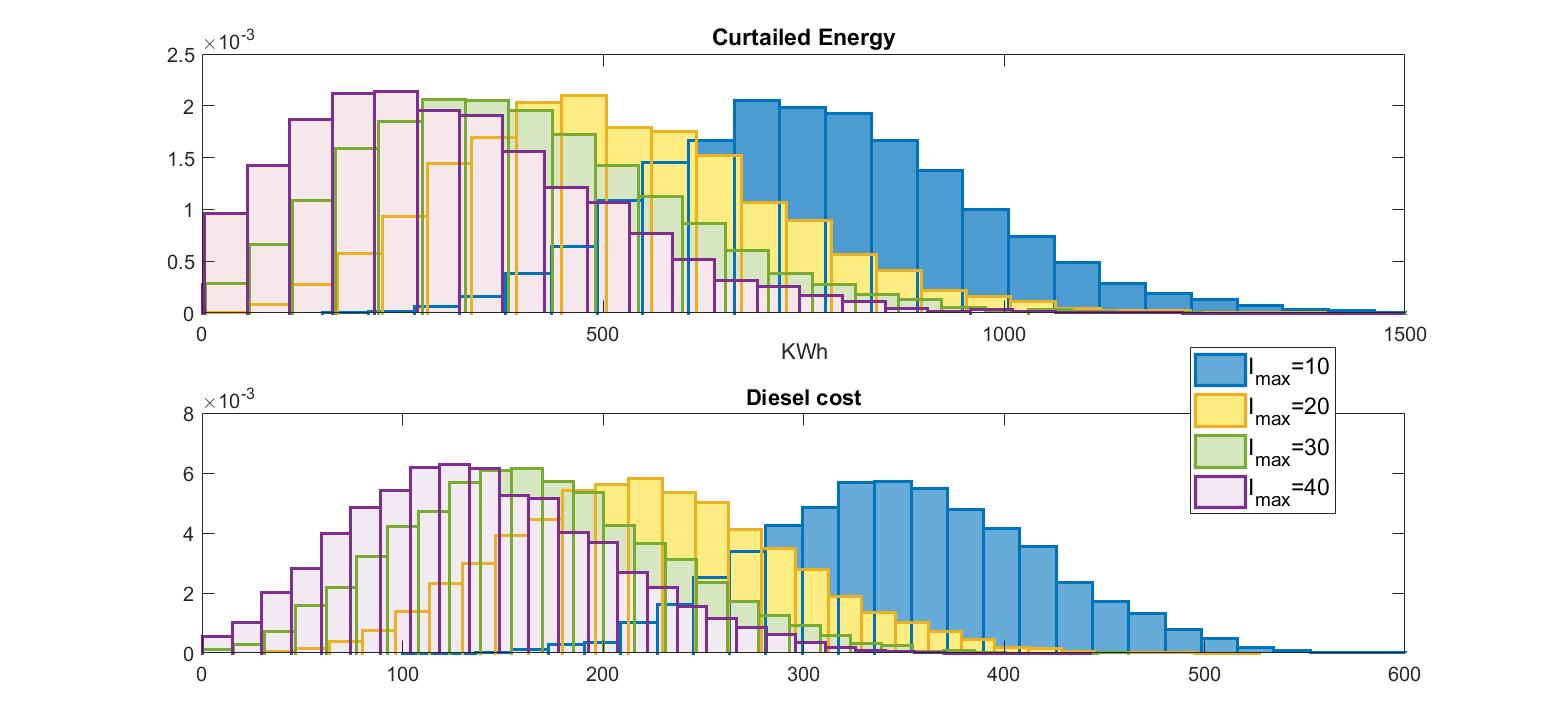
Figure 6: In the figure above we show histograms for different levels of battery capacity. In the top panel we display the estimated probability density of the curtailed energy, while in the bottom panel the estimated density of the cost of operating the diesel generator. Notice that the decrease in cost and curtailed energy per KWh of additional capacity is smaller for high capacity batteries.

We show now how to infer information about the optimal sizing of the battery, minimizing the trade off between the installation cost of a bigger battery and the reduced use of the diesel generator. Consider however that including battery ageing in the stochastic control problem is outside the scope of this paper but rather in this section we present only a post-optimization analysis. Assuming that the microgrid runs under similar conditions for the next 10 years, we can quickly estimate the total throughput of energy for the different battery capacities. Consider now that a battery has not an infinite lifetime, but rather it should be scrapped after equivalent 4000 cycles (amount of energy for one full charge and discharge). Under the previous assumptions, we can compute how many batteries would be necessary to cover the next 10 years of operations. Similarly, using the data relative to the usage of diesel generator for different levels of capacity, we can compute the operating cost of the diesel generator over the same time period. Further exploiting the assumption about the lifetime of a battery, we obtain the cost of running the grid for 10 years as a function of the number of batteries. To conclude, assuming a linear cost of 400 ${€\,$}/KWhofcapacity,weworkouttheinstallationcostofthedifferent-sizestoragedevices.\par Oncethisinformationiscollectedwesearchfortheminimumofthesumofinstallationandrunningcostand,inturn,wecomputetheoptimalcapacity.Figure\ref{fig:opt_battery},ontheleft,displaysagraphicalsummaryoftheprocedurejustdescribedandshowsthatinourproblemtheoptimalsizeofthebatteryis$14$KWhunderthecurrentsetofassumptions.Further,westudyhowmuchourresultisaffectedbythecostperKWhofcapacity,repeatingtheprocedureabove.Wefindthat,asexpected,ascostincreasethesizeoftheoptimalbatterydecreases.Figure\text{<span class="ltx\_ref ltx\_missing\_label ltx\_font\_italic ltx\_ref\_self">LABEL:fig:opt\_battery</span>},ontheright,displayssuchbehaviour.\text{Figure 7Figure 77Figure 77Inthefigureabovewecomputethetotalcostofinstallingandrunningthegridfortenyears,assumingwerepla}$