]pedro.figueroaromero@monash.edu
Almost Markovian processes from closed dynamics
Abstract
It is common, when dealing with quantum processes involving a subsystem of a much larger composite closed system, to treat them as effectively memory-less (Markovian). While open systems theory tells us that non-Markovian processes should be the norm, the ubiquity of Markovian processes is undeniable. Here, without resorting to the Born-Markov assumption of weak coupling or making any approximations, we formally prove that processes are close to Markovian ones, when the subsystem is sufficiently small compared to the remainder of the composite, with a probability that tends to unity exponentially in the size of the latter. We also show that, for a fixed global system size, it may not be possible to neglect non-Markovian effects when the process is allowed to continue for long enough. However, detecting non-Markovianity for such processes would usually require non-trivial entangling resources. Our results have foundational importance, as they give birth to almost Markovian processes from composite closed dynamics, and to obtain them we introduce a new notion of equilibration that is far stronger than the conventional one and show that this stronger equilibration is attained.
Suggested keywords
1 Introduction
The quest towards understanding how thermodynamics emerges from quantum theory has seen a great deal of recent progress [1, 2]. Most prominently, the conundrum of how to recover irreversible phenomena that obey the second law of thermodynamics, starting from reversible and recurrent Schrödinger dynamics, has been rectified by considering an analogous dynamical equilibrium. This is known generically as equilibration on average; it implies that time-dependent quantum properties evolve towards a certain fixed equilibrium value, and stay close to it for most times 111 Even stronger (but usually the one of interest) is the notion of equilibration in a finite time interval. The corresponding statement for a physical system replaces the term equilibration with thermalisation and the equilibrium state with a thermal state. For detail see e.g. [1].
Equilibration on average has been widely studied for small non-degenerate subsystems of larger closed systems, which are usually taken to be (quasi) isolated, and for particular models (see e.g. [3]). In a typical setup, the closed dynamics of a system and environment, as illustrated in Fig. 1(a), is considered. Remarkably, it can be shown that the expectation value for any observable on the system alone lies in the neighbourhood of its time-averaged value for almost all times [Fig. 1(b)]. Yet, such equilibration results, in full generality, remain unsolved [1]; in particular, it is unknown whether they extend to correlations between observables at different times.
To see this, consider the case depicted in Fig. 1(c), where the subsystem is interrogated (by measuring, or otherwise manipulating it) multiple times as it evolves with the remainder of the closed system, which acts as an environment. In such a scenario, the flow of information between interventions must be taken into account; in particular, there may be intrinsic temporal correlations mediated by the environment, in other words memory built up within the dynamics itself, independently of the external interventions, which are the hallmark of so-called non-Markovian dynamics. Equilibration on average says that the process erases the information contained in the initial state of the system; however, there may still be non-Markovian memory of the initial state encoded in the temporal correlations between observables. It is therefore an open question whether this information is truly scrambled by the process and therefore inaccessible to the system at long times. Such memoryless dynamics are anticipated for the subparts of closed many-body dynamics [4]. This scrambling of information in correlations would represent a stronger notion of equilibration than the usual one, which only considers statistics of individual observables at a given time. Moreover, the absence of memory effects would generically imply the usual kind of equilibration.
Searching for this stronger notion of equilibration is not physically unmotivated. While, strictly speaking, non-Markovian dynamics is the norm for subsystems of a closed system evolving with a time-independent Hamiltonian [5, 6], Markov approximations are commonly made throughout physics (and elsewhere) to good effect. However, the standard approach to making this approximation in open quantum systems theory involves a series of assumptions about weak interactions with an environment sufficiently large and ergodic that the memory of past interactions gets practically lost [7, 8]; this is mathematically equivalent (through an analogue of Stinespring’s dilation theorem) to continually refreshing (discarding and replacing) the environment’s state [9], i.e., artificially throwing away information from the environment (see Fig. 2). In reality, this is not usually how a closed system evolves, leading to the question: In the general case, how does dissipative Markovian dynamics emerge from closed Schrödinger evolution? That this puzzle is similar to the ones concerning equilibration and thermalisation should not be too surprising, as thermalisation is often achieved by assuming a Markov process [10].
Here, we give an initial answer to this deep foundational question. We show that, for the class of evolutions given by the Haar measure (typically involving an interaction of the subsystem with a significant portion of the remainder), above a critical time scale the dynamics of a subsystem is exponentially close to a Markov process as a function of the relative size of the subsystem compared with the whole. Moreover, our result does not assume weak coupling between the system and the environment, and we do not employ any approximations. Specifically, we use averages over the unitary group together with the concentration of measure phenomenon [11, 12, 13, 14, 15] to determine when a subsystem dynamics might typically be close to Markovian. Our approach is broadly similar to that of Refs. [14, 16] both in spirit and in terms of the mathematical tools employed. In other words, our main result gives a mechanism for equilibration starting from closed dynamics without employing any approximations.
Our results are possible thanks to recent efforts towards the understanding of general quantum processes, culminating in the development of the process tensor framework [17, 18, 19], which allows for the complete and compact description of an open system’s evolution under the influence of a series of external manipulations or measurements [20, 21].
Crucially, the process tensor framework leads to an unambiguous distinction between Markovian and non-Markovian dynamics, analogous to the usual one for classical stochastic processes. In this sense, it subsumes other approaches to quantum non-Markovianity (when compared with respect to the same process), including those based on increasing trace-distance distinguishability [22]. It allows for a precise quantification of memory effects (including across multiple time points) [5], that we employ here as a natural setting to explore temporal correlations and the role that they play in a generalized, or strong, notion of equilibration.
2 Quantum processes with memory: the process tensor
We begin with the motivation of witnessing equilibration effects through a sequence of measurements on the system. We consider a closed environment-system () with finite dimensional Hilbert space initialised in a pure joint state . The system is acted on with an initial measurement operation followed by a series of subsequent measurement operations at a sequence of fixed times, between which it evolves unitarily with the environment ; these operations are represented by trace non-increasing completely positive (CP) maps, and they include information about how the system is affected by the measurement procedure. Our results also hold for more general operations than just measurements, including unitary transformations or any other experimental manipulations of the system, but we focus on the former in order to be concrete. This scenario is depicted in Fig. 1(c). Formally, a -step process tensor is a completely positive causal 222 Meaning that the output of a process tensor at time does not depend on deterministic inputs at later times . map from the set to output states, .
It must be stressed, however, that although experimental interventions play an important role in the reconstruction of a process through a generalized quantum process tomography, they do not determine its nature, i.e., the process tensor itself accounts precisely for the intrinsic dynamics occurring independently of the control of the experimenter. Moreover, like any other CP map, the process tensor can be expressed as a (many-body) quantum state through the Choi-Jamiołkowski isomorphism [23, 24, 21]. For a -step process tensor, the corresponding (normalized) Choi state can be obtained by swapping the system with one half of a maximally entangled state at each time [25]. The ancillary systems have Hilbert space dimension 333 The dimensions of each , must be fixed to to make the swap operator well defined. and the system is swapped with an subsystem at each time. With this convention, the Choi state of the process tensor can be seen to take the form
| (1) |
where all identity operators act on the ancillary systems, is the unitary operator that evolves the joint system following the control operation at time and the are swap operators between system and the ancillary system . The corresponding quantum circuit is depicted in Fig. 3.
Throughout the paper, we write for the Choi state of a -step process unless otherwise specified.
3 An unambiguous measure of non-Markovianity
Among other important properties, the process tensor leads to a well-defined Markov criterion, from which it is possible to construct a family of operationally meaningful measures of non-Markovianity, many of which can be stated simply as distances between a process tensor’s Choi state and that of a corresponding Markovian one . The latter must take the form of a tensor product of quantum maps connecting adjacent pairs of time steps: [25].
In [5], a such measure of non-Markovianity was first introduced through the relative entropy between a process and its corresponding Markovian one, , minimized over the latter. Here, however, in analogy with other studies on equilibration, we choose the measure of non-Markovianity defined in terms of the trace distance as
| (2) |
where is the trace norm (or Schatten 1-norm); in particular, this is related to relative entropy through the so-called quantum Pinsker inequality, . The trace distance is a natural choice, as it represents an important distinguishability measure and has played a central role in the discovery of several major results on typicality [14] and equilibration [1, 26, 16] (or lack thereof, e.g. [27]). It has an experimental importance for comparing quantum processes [28] and is naturally related to other important distinguishability measures such as the diamond norm or the fidelity. However, it is important to point out that the above measure is fundamentally different (and more powerful) than other measures of non-Markovianity that have been proposed in recent years, including one that employs trace distance [22]. The measure we use here captures all non-Markovian features across multiple time steps and provides an operational meaning for non-Markovianity. Equipped with this measure, we are in a position to determine what value it takes for a typical process, answering the question posed at the beginning of this manuscript.
4 Typicality of Markovian processes
In order to quantify non-Markovianity, as defined in Eq. (2), for a typical process, we first need a concrete notion of typicality. There are many ways in which one could sample from the space of quantum processes, but as we are particularly interested in the typicality (or absence thereof) of Markovian processes independently of ad-hoc assumptions like weak coupling, we would like our measure to assign non-vanishing probabilities to mathematically generic unitary dynamics on the closed system.
Here, we achieve this by sampling the evolution from the unitarily invariant probability measure, the so-called Haar measure. This has the additional advantage of allowing us to average by means of random matrix theory techniques [29, 15, 30, 31, 32] and leads to the relatively straightforward application of concentration of measure results [11, 12, 13]. Specifically, we use the Haar measure to sample two distinct types of evolution:
-
1.
Random interaction: All independently chosen,
-
2.
Constant interaction: ,
where represents the closed (unitary) evolution between the application of measurement operation and , as depicted in Fig. 1(c); the entire set enters into the process tensor through Eq. (1). In the first case, the global system will quickly explore its entire (pure) state space for any initial state. The second case corresponds more closely to what one might expect for a truly closed system, where the Hamiltonian remains the same throughout the process. These correspond to two extremes; more generally, the dynamics from step to step may be related but not identical.
We highlight that under this sampling method, and thus this notion of typicality, the interaction or information flow between all parts of the whole system plus environment is relevant, i.e. no parts of the environment dimension are superfluous. We will now show that this kind of dynamics is almost always close to Markovian.
4.1 Main result
Our main result states that, for a randomly sampled -step quantum process undergone by a -dimensional subsystem of a larger -dimensional composite, the probability for the non-Markovianity to exceed a function of , and , that becomes very small in the large limit, itself becomes small in that limit. Precisely, we prove that, for an arbitrary ,
| (3) |
where with for a constant interaction process and for a random interaction process. The function is an upper bound on the expected non-Markovianity whose details depend on the way in which processes are sampled.
The proof is presented in full in Appendix E, and it can be outlined as follows: we first bound the difference between for two different processes in terms of the distance between the unitaries used to generate them; Levy’s lemma [11, 13, 14] then states that the fraction of processes with non-Markovianity more than away from the expectation value (which we upper-bound by ) is bounded by a concentration function. By considering the geometry of the spaces of unitaries we are sampling from, we are able to use the exponential function appearing on the right hand side of Eq. (3). This implies that our result holds particularly for this class of evolutions where all parts of system and environment effectively interact, in contrast with some commonly considered open systems models.
Our result is meaningful when both and are small; the latter is fulfilled in the small subsystem or large environment limit, which in our setting means . We may also state the minimal value for that, assuming the large environment limit, renders both sides small, i.e., such that ; this is fulfilled for 444Similar to [14], here we look for an such that and . A geometrical cartoon to illustrate the result is presented in Fig. 4.
This is the case because the upper bound is given by
| (4) |
with , . The size of depends entirely on the size of the average purity of the process tensor , which we have computed analytically for the case of Haar-randomly sampled evolutions (which equivalently could be sampled from -unitary designs [33, 34], as we will discuss below) in Appendix F.
The purity is a quantifier of the mixedness (uniformity of eigenvalues) of a positive operator. When computed on reduced states of bipartite systems it can also serve as a quantifier of entanglement. In Appendix D, we analytically compute the expected purity of the Choi state of a process tensor in both the constant and the random interaction pictures, which can be directly translated as a quantifier for noisiness of the quantum process itself and entanglement between system and environment. The expressions take the form
| (5) |
for the random interaction picture and
| (6) |
in the constant interaction case, where is the symmetric group over elements, is known as the Weingarten function [30], is a product of entries of depending on permutations and is a product, scaling with , of monomials in and depending on permutations and .
4.2 Limiting cases
In both the constant and random interaction cases, is a well-behaved rational function of , and . Eq. (6) takes a non-trivial form mainly because of the function (which is intrinsic to the Haar-unitary averaging in the constant interaction picture). However, due to results found in [30, 31], we can still study analytically the behaviour of the bound for both cases in the two following limits.
In the large environment limit,
| (7) |
which corresponds to the purity of the maximally mixed state. Note that the averaging occurs after computing the purity; that is, independently of which case is considered. Every process sampled will be indistinguishable from the maximally noisy (and hence Markovian) one, with probability that tends to one as is increased:
| (8) |
Furthermore, from Eq. (5) it is seen that it does so at a rate in the random interaction case.
The other interesting limiting case is the one where the dimension is fixed, but the number of time steps is taken to be very large. The resulting process encodes all high order correlation functions between observables over a long period of time. Again for both cases, the expected purity in this limit goes as
| (9) |
which corresponds to the maximally mixed purity of the environment. This implies that the Choi state of the full unitary process is maximally entangled between and . In this limit, we get correspondingly
| (10) |
meaning that nothing can be said about typical non-Markovianity; a typical process in this limit could be highly non-Markovian. Indeed, we expect this to be the case, since the finite-dimensional space will have a finite recurrence time.
Both our main result in Eq. (3), and the bound on non-Markovianity, Eq. (4), generalize well-known results for quantum states, i.e., when . In this case, our main result reduces to the usual one for the typicality of maximally mixed states (or bipartite maximally entangled states), with (see e.g. [35]). As we also detail in Appendix F, when we take the Haar measure, in either case, we recover the average purity
| (11) |
where , as found in [36, 37, 38, 39, 15, 40, 41]. This then leads to
| (12) |
which goes as when , and is also a standard result [35].
4.3 Numerical examples
To support our results, we sampled Choi states numerically in the random interaction case and computed their corresponding average non-Markovianity as a function of environment dimension for a fixed system dimension , obtaining the behaviour shown in Fig. 5. For constant interaction the numerical results are practically indistinguishable from those in the random case, but as mentioned, the analytical bound is much harder to compute exactly. This suggests that either a simpler bound exists or that it might be possible to simplify the one we have obtained. As expected, our numerical results fall within the bound and they behave similarly; we notice that the bound in general seems to be somewhat loose, and become loosest when , implying that non-Markovianity might be hard to detect even when not strictly in the large environment limit. However, it does saturate rapidly as increases.
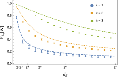
So far, our results are valid for process tensors constructed with Haar random unitaries at evenly spaced steps; we are effectively considering a strong interaction between system and environment which rapidly scrambles quantum information in both [33]. The mechanism for equilibration is precisely that of dephasing [1], or effectively, the scrambling of information on the initial state of the system. This suggests that, even when timescales will differ with the type of evolution considered, most physical evolutions fall within our result, with e.g. a weaker behavior in .
Our results could potentially be extended to their analogues sampled from unitary -designs, approximate or otherwise [43], that reproduce the Haar distribution up to the -th moment. As mentioned above, our expression for the upper bound in Eq. (4) is identical for samples from a -designs, and, if the non-Markovianity could be approximated by a polynomial function of , Eq. (3) would also hold for -designs with large enough [44]. This type of distribution has recently been shown to be approximated by a wide class of physical evolutions [45]. In particular, the unitary circuits involved in complex quantum computations typically look Haar random [34]; if it holds in this case, our result would therefore suggest that the behaviour of components of a quantum computer would not typically exhibit non-Markovian memory (at least due to the computation itself). Furthermore, even when it’s known that ensembles for time-independent Hamiltonians cannot strictly become Haar random [33], certain complex Hamiltonian systems can be treated as random up to a certain Haar-moment via unitary designs [45].
These issues should be investigated further, however, we will now show that our results still hold at a coarse-grained level, where the intermediate dynamics corresponds to products of Haar random unitaries, which are not themselves Haar random.
5 Observing non-Markovianity
The choice of unitaries going into the process tensor in the previous sections (in our case drawn from the Haar measure), dictates a time scale for the system, up to a freely chosen energy scale. However, we can straightforwardly construct process tensors on a longer, coarse-grained time scale by simply allowing the system to evolve (with an identity operation) between some subset of time steps. In fact, process tensors at all time scales should be related in this way to an underlying process tensor with an infinite number of steps [46].
To see that our main result directly applies to any process tensor that can be obtained through coarse graining, we again consider the definition of our non-Markovianity measure, given in Eq. (2). Consider the coarser grained process tensor , where a subset of control operations are replaced by identity operations (i.e., the system is simply left to evolve). Letting , we have
| (13) |
since the set of allowed strictly contains the allowed at the finer-grained level. This renders the new process less distinguishable from a Markovian one, i.e., coarse-graining can only make processes more Markovian.
The physical intuition behind this result is that the amount of information which can be encoded in a coarse grained process tensor is strictly less than that in its parent process tensor. In fact, this is a key feature of non-Markovian memory: the memory should decrease under coarse graining. On the other hand, due to the same reasoning, we cannot say anything about finer-grained dynamics. One approach to tackling this issue would be to choose a different sampling procedure which explicitly takes scales into account. However, we leave this for future work.
There is another important limitation for observing non-Markovianity. The operational interpretation of the trace distance, discussed in the previous section, implies that observing non-Markovianity requires applying a measurement that is an eigen-projector operator of . The optimal measurement will, in general, be entangled across all time steps. In practice, this is hard to achieve and typically one considers a sequence of local measurements . In general, for an any set of measurements we can define a restricted measure of non-Markovianity detectable with that set: , which means that the detectable non-Markovianity will be smaller. This is akin to the eigenstate thermalization hypothesis [47], where all eigenstates of a physical Hamiltonian look uniformally distributed with respect to most ‘physically reasonable’ observables. In our setting, this means that looking for non-Markovianity with observables that are local in time – i.e., ‘physically reasonable’ – we find almost no temporal correlations.
The locality constraint, along with monotonicity of non-Markovianity under coarse graining, have further important consequences for a broad class of open systems studies where master equations are employed [48]. Since master equations usually only account for two-point correlations with local measurements, they will be insensitive to most of the temporal correlations being accounted for by our measure, leading to an even greater likelihood for their descriptions to be Markovian. We now discuss the broader implications of our results.
6 Discussions and Conclusions
Our results imply that it is fundamentally hard to observe non-Markovianity in a typical process and thus go some way to explaining the overwhelming success of Markovian theories.
Specifically, we have shown that, even when interacting strongly with the wider composite system, a subsystem will typically undergo highly Markovian dynamics when the rest of the system has a sufficiently large dimension, and that the probability to be significantly non-Markovian vanishes with the latter. Our main result formalizes the notion that in the large environment limit a quantum process, taken uniformly at random, will be almost Markovian with very high probability. This corroborates the common understanding of the Born-Markov approximation [7, 8], but, crucially, we make no assumptions about weak coupling between and . Instead, in the Haar random interactions we consider, every part of the system typically interacts significantly with every part of . This is in contrast to many open systems models, even those with superficially infinite dimensional baths, where the effective dimension of the environment is relatively small [49]; it can always be bounded by a function of time scales in the system-environment Hamiltonian [50], which could be encoded in a bath spectral density. Our result is also more general than the scenario usually considered, since it accounts for interventions and thus the flow of information between and across multiple times.
While it may still be possible to observe non-Markovian behaviour at a time scale that is smaller than the fundamental time scale set by the chosen unitaries, Eq. (13) tells us that any coarse grained process will remain concentrated around the Markovian ones in the large environment limit. Otherwise, for larger and larger systems, one needs an ever increasing number of time steps, corresponding to higher order correlations, in order to increase the probability of witnessing non-Markovianity. However, even in this case, from the discussion in the previous section, we know that the measurement on this large number of times steps will be temporally entangled, which may also be difficult to achieve.
We have introduced a stronger notion of equilibration than the conventional one [1], so that strong equilibration implies weak equilibration. Our main result shows that it is possible to attain strong equilibration, where the information of the initial state of the system does not exist in multi-time correlations, much less expectation values at different times. Our result can be interpreted as a mechanism for equilibration and thermalisation. That is, we have shown that the dynamics of the system alone is almost Markovian, and such processes have well defined fixed points [51]. Even if we do not characterise the equilibrium state here, e.g. as done for quantum states under randomized local Hamiltonians [52], we may conclude that the state of the system approaches this fixed point and the expectation value for any observable will lie in the neighbourhood of the time-averaged value [as depicted in Fig. 1(b)] for most times. However, one point of departure between the two results is our reliance on Haar sampling.
More precisely, we have considered the case where the joint unitary evolution between each time step is drawn uniformly at random according to the Haar measure, for the two limiting cases of the random unitary operators at each step being the same or independent. This is, however, different from simply sampling the Choi state of the process Haar randomly. It is also not equivalent to picking Haar random states for the system at every time, as one would expect if the results of Ref. [14] were to hold independently at all times.
Nevertheless, tackling the issues we have pointed out, a notion of equilibration in general processes can potentially be made precise and other issues such as equilibration time scales can also be readily explored; the approach that we have presented constitutes a first significant step towards achieving this goal.
References
- Gogolin and Eisert [2016] C. Gogolin and J. Eisert, “Equilibration, thermalisation, and the emergence of statistical mechanics in closed quantum systems,” \bibfield journal \bibinfo journal Rep. Prog. Phys.\ \textbf \bibinfo volume 79,\ \bibinfo pages 056001 (\bibinfo year 2016).
- Goold et al. [2016] J. Goold, M. Huber, A. Riera, L. del Rio, and P. Skrzypczyk, “The role of quantum information in thermodynamics–a topical review,” \bibfield journal \bibinfo journal J. Phys. A: Math. Theor.\ \textbf \bibinfo volume 49,\ \bibinfo pages 143001 (\bibinfo year 2016).
- García-Pintos et al. [2017] L. P. García-Pintos, N. Linden, A. S. L. Malabarba, A. J. Short, and A. Winter, “Equilibration time scales of physically relevant observables,” \bibfield journal \bibinfo journal Phys. Rev. X\ \textbf \bibinfo volume 7,\ \bibinfo pages 031027 (\bibinfo year 2017).
- Srednicki [1999] M. Srednicki, “The approach to thermal equilibrium in quantized chaotic systems,” \bibfield journal \bibinfo journal J. Phys. A: Math. Gen.\ \textbf \bibinfo volume 32,\ \bibinfo pages 1163 (\bibinfo year 1999).
- Pollock et al. [2018a] F. A. Pollock, C. Rodríguez-Rosario, T. Frauenheim, M. Paternostro, and K. Modi, “Operational markov condition for quantum processes,” \bibfield journal \bibinfo journal Phys. Rev. Lett.\ \textbf \bibinfo volume 120,\ \bibinfo pages 040405 (\bibinfo year 2018\natexlaba).
- Arenz et al. [2015] C. Arenz, R. Hillier, M. Fraas, and D. Burgarth, “Distinguishing decoherence from alternative quantum theories by dynamical decoupling,” \bibfield journal \bibinfo journal Phys. Rev. A\ \textbf \bibinfo volume 92,\ \bibinfo pages 022102 (\bibinfo year 2015).
- Schlosshauer [2007] M. A. Schlosshauer, \emph \bibinfo title Decoherence and the Quantum-To-Classical Transition (Springer Berlin Heidelberg, 2007).
- de Vega and Alonso [2017] I. de Vega and D. Alonso, “Dynamics of non-Markovian open quantum systems,” \bibfield journal \bibinfo journal Rev. Mod. Phys.\ \textbf \bibinfo volume 89,\ \bibinfo pages 015001 (\bibinfo year 2017).
- Ciccarello [2017] F. Ciccarello, “Collision models in quantum optics,” \bibfield journal \bibinfo journal Quantum Meas. Quantum Metrol.\ \textbf \bibinfo volume 4,\ \bibinfo pages 53 (\bibinfo year 2017).
- Spohn and Lebowitz [2007] H. Spohn and J. L. Lebowitz, “Irreversible thermodynamics for quantum systems weakly coupled to thermal reservoirs,” in \emph \bibinfo booktitle Advances in Chemical Physics, edited by S. A. Rice (John Wiley & Sons, Ltd, 2007) pp. 109–142.
- Ledoux [2001] M. Ledoux, \emph \bibinfo title The Concentration of Measure Phenomenon, Mathematical surveys and monographs (American Mathematical Society, 2001).
- Milman and Schechtman [1986] V. D. Milman and G. Schechtman, \emph \bibinfo title Asymptotic Theory of Finite Dimensional Normed Spaces, Lecture Notes in Mathematics No. 1200 (Springer-Verlag, 1986).
- Boucheron et al. [2013] S. Boucheron, G. Lugosi, and P. Massart, \emph \bibinfo title Concentration Inequalities: A Nonasymptotic Theory of Independence (OUP Oxford, 2013).
- Popescu et al. [2006] S. Popescu, A. J. Short, and A. Winter, “Entanglement and the foundations of statistical mechanics,” \bibfield journal \bibinfo journal Nat. Phys.\ \textbf \bibinfo volume 2,\ \bibinfo pages 754 (\bibinfo year 2006).
- Li [2013] Y. Li, “Seminar 6 of selected topics in mathematical physics: Quantum information theory,” \urlprefix\@@endlink (\bibinfoyear 2013)\BibitemShutNoStop
- \citenamefontMasanes et al. [2013] \BibitemOpen\bibfieldauthor \bibinfoauthor \bibfnamefontL. \bibnamefontMasanes, \bibinfoauthor \bibfnamefontA. J. \bibnamefontRoncaglia, and \bibinfoauthor \bibfnamefontA. \bibnamefontAcín, \bibfieldtitle \enquote\bibinfotitle Complexity of energy eigenstates as a mechanism for equilibration, \href\doibase10.1103/PhysRevE.87.032137 \bibfieldjournal \bibinfojournal Phys. Rev. E \bibinfovolume 87, \bibinfopages 032137 (\bibinfoyear 2013)\BibitemShutNoStop
- \citenamefontChiribella et al. [2008] \BibitemOpen\bibfieldauthor \bibinfoauthor \bibfnamefontG. \bibnamefontChiribella, \bibinfoauthor \bibfnamefontG. M. \bibnamefontD’Ariano, and \bibinfoauthor \bibfnamefontP. \bibnamefontPerinotti, \bibfieldtitle \enquote\bibinfotitle Quantum circuit architecture, \href\doibase10.1103/PhysRevLett.101.060401 \bibfieldjournal \bibinfojournal Phys. Rev. Lett. \bibinfovolume 101, \bibinfopages 060401 (\bibinfoyear 2008)\BibitemShutNoStop
- \citenamefontChiribella et al. [2009] \BibitemOpen\bibfieldauthor \bibinfoauthor \bibfnamefontG. \bibnamefontChiribella, \bibinfoauthor \bibfnamefontG. M. \bibnamefontD’Ariano, and \bibinfoauthor \bibfnamefontP. \bibnamefontPerinotti, \bibfieldtitle \enquote\bibinfotitle Theoretical framework for quantum networks, \href\doibase10.1103/PhysRevA.80.022339 \bibfieldjournal \bibinfojournal Phys. Rev. A \bibinfovolume 80, \bibinfopages 022339 (\bibinfoyear 2009)\BibitemShutNoStop
- \citenamefontCosta and \citenamefontShrapnel [2016] \BibitemOpen\bibfieldauthor \bibinfoauthor \bibfnamefontF. \bibnamefontCosta and \bibinfoauthor \bibfnamefontS. \bibnamefontShrapnel, \bibfieldtitle \enquote\bibinfotitle Quantum causal modelling, \href\doibase10.1088/1367-2630/18/6/063032 \bibfieldjournal \bibinfojournal New J. Phys. \bibinfovolume 18, \bibinfopages 063032 (\bibinfoyear 2016)\BibitemShutNoStop
- \citenamefontModi [2012] \BibitemOpen\bibfieldauthor \bibinfoauthor \bibfnamefontK. \bibnamefontModi, \bibfieldtitle \enquote\bibinfotitle Operational approach to open dynamics and quantifying initial correlations, \href\doibase10.1038/srep00581 \bibfieldjournal \bibinfojournal Sci. Rep. \bibinfovolume 2, \bibinfopages 581 (\bibinfoyear 2012)\BibitemShutNoStop
- \citenamefontPollock et al. [2018b] \BibitemOpen\bibfieldauthor \bibinfoauthor \bibfnamefontF. A. \bibnamefontPollock, \bibinfoauthor \bibfnamefontC. \bibnamefontRodríguez-Rosario, \bibinfoauthor \bibfnamefontT. \bibnamefontFrauenheim, \bibinfoauthor \bibfnamefontM. \bibnamefontPaternostro, and \bibinfoauthor \bibfnamefontK. \bibnamefontModi, \bibfieldtitle \enquote\bibinfotitle Non-Markovian quantum processes: Complete framework and efficient characterization, \href\doibase10.1103/PhysRevA.97.012127 \bibfieldjournal \bibinfojournal Phys. Rev. A \bibinfovolume 97, \bibinfopages 012127 (\bibinfoyear 2018b)\BibitemShutNoStop
- \citenamefontBreuer et al. [2016] \BibitemOpen\bibfieldauthor \bibinfoauthor \bibfnamefontH.-P. \bibnamefontBreuer, \bibinfoauthor \bibfnamefontE.-M. \bibnamefontLaine, \bibinfoauthor \bibfnamefontJ. \bibnamefontPiilo, and \bibinfoauthor \bibfnamefontB. \bibnamefontVacchini, \bibfieldtitle \enquote\bibinfotitle Colloquium: Non-Markovian dynamics in open quantum systems, \href\doibase10.1103/RevModPhys.88.021002 \bibfieldjournal \bibinfojournal Rev. Mod. Phys. \bibinfovolume 88, \bibinfopages 021002 (\bibinfoyear 2016)\BibitemShutNoStop
- \citenamefontChoi [1975] \BibitemOpen\bibfieldauthor \bibinfoauthor \bibfnamefontM.-D. \bibnamefontChoi, \bibfieldtitle \enquote\bibinfotitle Completely positive linear maps on complex matrices, \href\doibase10.1016/0024-3795(75)90075-0 \bibfieldjournal \bibinfojournal Linear Algebra Its Appl. \bibinfovolume 10, \bibinfopages 285 (\bibinfoyear 1975)\BibitemShutNoStop
- \citenamefontJamiołkowski [1972] \BibitemOpen\bibfieldauthor \bibinfoauthor \bibfnamefontA. \bibnamefontJamiołkowski, \bibfieldtitle \enquote\bibinfotitle Linear transformations which preserve trace and positive semidefiniteness of operators, \href\doibase10.1016/0034-4877(72)90011-0 \bibfieldjournal \bibinfojournal Rep. Math. Phys. \bibinfovolume 3, \bibinfopages 275 (\bibinfoyear 1972)\BibitemShutNoStop
- \citenamefontMilz et al. [2017a] \BibitemOpen\bibfieldauthor \bibinfoauthor \bibfnamefontS. \bibnamefontMilz, \bibinfoauthor \bibfnamefontF. A. \bibnamefontPollock, and \bibinfoauthor \bibfnamefontK. \bibnamefontModi, \bibfieldtitle \enquote\bibinfotitle An introduction to operational quantum dynamics, \href\doibase10.1142/S1230161217400169 \bibfieldjournal \bibinfojournal Open Syst. Inf. Dyn. \bibinfovolume 24, \bibinfopages 1740016 (\bibinfoyear 2017a)\BibitemShutNoStop
- \citenamefontShort and \citenamefontFarrelly [2012] \BibitemOpen\bibfieldauthor \bibinfoauthor \bibfnamefontA. J. \bibnamefontShort and \bibinfoauthor \bibfnamefontT. C. \bibnamefontFarrelly, \bibfieldtitle \enquote\bibinfotitle Quantum equilibration in finite time, \href\doibase10.1088/1367-2630/14/1/013063 \bibfieldjournal \bibinfojournal New J. Phys. \bibinfovolume 14, \bibinfopages 013063 (\bibinfoyear 2012)\BibitemShutNoStop
- \citenamefontGogolin et al. [2011] \BibitemOpen\bibfieldauthor \bibinfoauthor \bibfnamefontC. \bibnamefontGogolin, \bibinfoauthor \bibfnamefontM. P. \bibnamefontMüller, and \bibinfoauthor \bibfnamefontJ. \bibnamefontEisert, \bibfieldtitle \enquote\bibinfotitle Absence of thermalization in nonintegrable systems, \href\doibase10.1103/PhysRevLett.106.040401 \bibfieldjournal \bibinfojournal Phys. Rev. Lett. \bibinfovolume 106, \bibinfopages 040401 (\bibinfoyear 2011)\BibitemShutNoStop
- \citenamefontGilchrist et al. [2005] \BibitemOpen\bibfieldauthor \bibinfoauthor \bibfnamefontA. \bibnamefontGilchrist, \bibinfoauthor \bibfnamefontN. K. \bibnamefontLangford, and \bibinfoauthor \bibfnamefontM. A. \bibnamefontNielsen, \bibfieldtitle \enquote\bibinfotitle Distance measures to compare real and ideal quantum processes, \href\doibase10.1103/PhysRevA.71.062310 \bibfieldjournal \bibinfojournal Phys. Rev. A \bibinfovolume 71, \bibinfopages 062310 (\bibinfoyear 2005)\BibitemShutNoStop
- \citenamefontZhang [2014] \BibitemOpen\bibfieldauthor \bibinfoauthor \bibfnamefontL. \bibnamefontZhang, \bibfieldtitle \enquote\bibinfotitle Matrix integrals over unitary groups: An application of Schur-Weyl duality, \hrefhttps://arxiv.org/abs/1408.3782 \bibfieldjournal \bibinfojournal arXiv:1408.3782 (\bibinfoyear 2014)\BibitemShutNoStop
- \citenamefontGu [2013] \BibitemOpen\bibfieldauthor \bibinfoauthor \bibfnamefontY. \bibnamefontGu, \bibinfotitle Moments of Random Matrices and. Weingarten Functions, \hrefhttp://hdl.handle.net/1974/8241 Master’s thesis, \bibinfoschool Queen’s University, \bibinfoaddress Ontario, Canada (\bibinfoyear 2013)\BibitemShutNoStop
- \citenamefontCollins and \citenamefontŚniady [2006] \BibitemOpen\bibfieldauthor \bibinfoauthor \bibfnamefontB. \bibnamefontCollins and \bibinfoauthor \bibfnamefontP. \bibnamefontŚniady, \bibfieldtitle \enquote\bibinfotitle Integration with respect to the Haar measure on unitary, orthogonal and symplectic group, \href\doibase10.1007/s00220-006-1554-3 \bibfieldjournal \bibinfojournal Commun. Math. Phys. \bibinfovolume 264, \bibinfopages 773 (\bibinfoyear 2006)\BibitemShutNoStop
- \citenamefontPuchała and \citenamefontMiszczak [2017] \BibitemOpen\bibfieldauthor \bibinfoauthor \bibfnamefontZ. \bibnamefontPuchała and \bibinfoauthor \bibfnamefontJ. A. \bibnamefontMiszczak, \bibfieldtitle \enquote\bibinfotitle Symbolic integration with respect to the Haar measure on the unitary groups, \href\doibase10.1515/bpasts-2017-0003 \bibfieldjournal \bibinfojournal Bull. Pol. Acad. Sci. Tech. Sci. \bibinfovolume 65, \bibinfopages 21 (\bibinfoyear 2017)\BibitemShutNoStop
- \citenamefontRoberts and \citenamefontYoshida [2017] \BibitemOpen\bibfieldauthor \bibinfoauthor \bibfnamefontD. A. \bibnamefontRoberts and \bibinfoauthor \bibfnamefontB. \bibnamefontYoshida, \bibfieldtitle \enquote\bibinfotitle Chaos and complexity by design, \href\doibase10.1007/JHEP04(2017)121 \bibfieldjournal \bibinfojournal J. High Energy Phys. \bibinfovolume 2017, \bibinfopages 121 (\bibinfoyear 2017)\BibitemShutNoStop
- \citenamefontBrandão et al. [2016] \BibitemOpen\bibfieldauthor \bibinfoauthor \bibfnamefontF. \bibnamefontBrandão, \bibinfoauthor \bibfnamefontA. W. \bibnamefontHarrow, and \bibinfoauthor \bibfnamefontM. \bibnamefontHorodecki, \bibfieldtitle \enquote\bibinfotitle Local random quantum circuits are approximate polynomial-designs, \href\doibase10.1007/s00220-016-2706-8 \bibfieldjournal \bibinfojournal Commun. Math. Phys. \bibinfovolume 346, \bibinfopages 397 (\bibinfoyear 2016)\BibitemShutNoStop
- \citenamefontGläßle [2013] \BibitemOpen\bibfieldauthor \bibinfoauthor \bibfnamefontT. \bibnamefontGläßle, \href@noop \enquote\bibinfotitle Seminar 8 of selected topics in mathematical physics: Quantum information theory, \bibinfohowpublished \urlhttp://www.mpmueller.net/seminar/talk8.pdf (\bibinfoyear 2013)\BibitemShutNoStop
- \citenamefontLubkin [1978] \BibitemOpen\bibfieldauthor \bibinfoauthor \bibfnamefontE. \bibnamefontLubkin, \bibfieldtitle \enquote\bibinfotitle Entropy of an n-system from its correlation with a k-reservoir, \href\doibase10.1063/1.523763 \bibfieldjournal \bibinfojournal J. Math. Phys. \bibinfovolume 19, \bibinfopages 1028 (\bibinfoyear 1978)\BibitemShutNoStop
- \citenamefontPage [1993] \BibitemOpen\bibfieldauthor \bibinfoauthor \bibfnamefontD. N. \bibnamefontPage, \bibfieldtitle \enquote\bibinfotitle Average entropy of a subsystem, \href\doibase10.1103/PhysRevLett.71.1291 \bibfieldjournal \bibinfojournal Phys. Rev. Lett. \bibinfovolume 71, \bibinfopages 1291 (\bibinfoyear 1993)\BibitemShutNoStop
- \citenamefontLloyd and \citenamefontPagels [1988] \BibitemOpen\bibfieldauthor \bibinfoauthor \bibfnamefontS. \bibnamefontLloyd and \bibinfoauthor \bibfnamefontH. \bibnamefontPagels, \bibfieldtitle \enquote\bibinfotitle Complexity as thermodynamic depth, \href\doibase10.1016/0003-4916(88)90094-2 \bibfieldjournal \bibinfojournal Ann. Phys. New York \bibinfovolume 188, \bibinfopages 186 (\bibinfoyear 1988)\BibitemShutNoStop
- \citenamefontScott and \citenamefontCaves [2003] \BibitemOpen\bibfieldauthor \bibinfoauthor \bibfnamefontA. J. \bibnamefontScott and \bibinfoauthor \bibfnamefontC. M. \bibnamefontCaves, \bibfieldtitle \enquote\bibinfotitle Entangling power of the quantum baker’s map, \href\doibase10.1088/0305-4470/36/36/308 \bibfieldjournal \bibinfojournal J. Phys. A: Math. Gen. \bibinfovolume 36, \bibinfopages 9553 (\bibinfoyear 2003)\BibitemShutNoStop
- \citenamefontGiraud [2007] \BibitemOpen\bibfieldauthor \bibinfoauthor \bibfnamefontO. \bibnamefontGiraud, \bibfieldtitle \enquote\bibinfotitle Purity distribution for bipartite random pure states, \href\doibase10.1088/1751-8113/40/49/f03 \bibfieldjournal \bibinfojournal J. Phys. A: Math. Theor. \bibinfovolume 40, \bibinfopages F1053 (\bibinfoyear 2007)\BibitemShutNoStop
- \citenamefontPasquale et al. [2012] \BibitemOpen\bibfieldauthor \bibinfoauthor \bibfnamefontA. D. \bibnamefontPasquale, \bibinfoauthor \bibfnamefontP. \bibnamefontFacchi, \bibinfoauthor \bibfnamefontV. \bibnamefontGiovannetti, \bibinfoauthor \bibfnamefontG. \bibnamefontParisi, \bibinfoauthor \bibfnamefontS. \bibnamefontPascazio, and \bibinfoauthor \bibfnamefontA. \bibnamefontScardicchio, \bibfieldtitle \enquote\bibinfotitle Statistical distribution of the local purity in a large quantum system, \href\doibase10.1088/1751-8113/45/1/015308 \bibfieldjournal \bibinfojournal J. Phys. A: Math. Theor. \bibinfovolume 45, \bibinfopages 015308 (\bibinfoyear 2012)\BibitemShutNoStop
- \citenamefontMezzadri [2007] \BibitemOpen\bibfieldauthor \bibinfoauthor \bibfnamefontF. \bibnamefontMezzadri, \bibfieldtitle \enquote\bibinfotitle How to generate random matrices from the classical compact groups, \hrefhttps://www.ams.org/journals/notices/200705/fea-mezzadri-web.pdf \bibfieldjournal \bibinfojournal Notices of the AMS \bibinfovolume 54, \bibinfopages 592 (\bibinfoyear 2007)\BibitemShutNoStop
- \citenamefontCotler et al. [2017] \BibitemOpen\bibfieldauthor \bibinfoauthor \bibfnamefontJ. \bibnamefontCotler, \bibinfoauthor \bibfnamefontN. \bibnamefontHunter-Jones, \bibinfoauthor \bibfnamefontJ. \bibnamefontLiu, and \bibinfoauthor \bibfnamefontB. \bibnamefontYoshida, \bibfieldtitle \enquote\bibinfotitle Chaos, complexity, and random matrices, \href\doibase10.1007/JHEP11(2017)048 \bibfieldjournal \bibinfojournal J. High Energy Phys. \bibinfovolume 2017, \bibinfopages 48 (\bibinfoyear 2017)\BibitemShutNoStop
- \citenamefontLow [2009] \BibitemOpen\bibfieldauthor \bibinfoauthor \bibfnamefontR. A. \bibnamefontLow, \bibfieldtitle \enquote\bibinfotitle Large deviation bounds for k-designs, \href\doibase10.1098/rspa.2009.0232 \bibfieldjournal \bibinfojournal Proc. R. Soc. A \bibinfovolume 465, \bibinfopages 3289 (\bibinfoyear 2009)\BibitemShutNoStop
- \citenamefontNakata et al. [2017] \BibitemOpen\bibfieldauthor \bibinfoauthor \bibfnamefontY. \bibnamefontNakata, \bibinfoauthor \bibfnamefontC. \bibnamefontHirche, \bibinfoauthor \bibfnamefontM. \bibnamefontKoashi, and \bibinfoauthor \bibfnamefontA. \bibnamefontWinter, \bibfieldtitle \enquote\bibinfotitle Efficient quantum pseudorandomness with nearly time-independent Hamiltonian dynamics, \href\doibase10.1103/PhysRevX.7.021006 \bibfieldjournal \bibinfojournal Phys. Rev. X \bibinfovolume 7, \bibinfopages 021006 (\bibinfoyear 2017)\BibitemShutNoStop
- \citenamefontMilz et al. [2017b] \BibitemOpen\bibfieldauthor \bibinfoauthor \bibfnamefontS. \bibnamefontMilz, \bibinfoauthor \bibfnamefontF. \bibnamefontSakuldee, \bibinfoauthor \bibfnamefontF. A. \bibnamefontPollock, and \bibinfoauthor \bibfnamefontK. \bibnamefontModi, \bibfieldtitle \enquote\bibinfotitle Kolmogorov extension theorem for (quantum) causal modelling and general probabilistic theories, \hrefhttps://arxiv.org/abs/1712.02589 \bibfieldjournal \bibinfojournal arXiv:1712.02589 (\bibinfoyear 2017b)\BibitemShutNoStop
- \citenamefontAnza et al. [2018] \BibitemOpen\bibfieldauthor \bibinfoauthor \bibfnamefontF. \bibnamefontAnza, \bibinfoauthor \bibfnamefontC. \bibnamefontGogolin, and \bibinfoauthor \bibfnamefontM. \bibnamefontHuber, \bibfieldtitle \enquote\bibinfotitle Eigenstate thermalization for degenerate observables, \href\doibase10.1103/PhysRevLett.120.150603 \bibfieldjournal \bibinfojournal Phys. Rev. Lett. \bibinfovolume 120, \bibinfopages 150603 (\bibinfoyear 2018)\BibitemShutNoStop
- \citenamefontPollock and \citenamefontModi [2018] \BibitemOpen\bibfieldauthor \bibinfoauthor \bibfnamefontF. A. \bibnamefontPollock and \bibinfoauthor \bibfnamefontK. \bibnamefontModi, \bibfieldtitle \enquote\bibinfotitle Tomographically reconstructed master equations for any open quantum dynamics, \href\doibase10.22331/q-2018-07-11-76 \bibfieldjournal \bibinfojournal Quantum \bibinfovolume 2, \bibinfopages 76 (\bibinfoyear 2018)\BibitemShutNoStop
- \citenamefontTamascelli et al. [2018] \BibitemOpen\bibfieldauthor \bibinfoauthor \bibfnamefontD. \bibnamefontTamascelli, \bibinfoauthor \bibfnamefontA. \bibnamefontSmirne, \bibinfoauthor \bibfnamefontS. F. \bibnamefontHuelga, and \bibinfoauthor \bibfnamefontM. B. \bibnamefontPlenio, \bibfieldtitle \enquote\bibinfotitle Nonperturbative treatment of non-Markovian dynamics of open quantum systems, \href\doibase10.1103/PhysRevLett.120.030402 \bibfieldjournal \bibinfojournal Phys. Rev. Lett. \bibinfovolume 120, \bibinfopages 030402 (\bibinfoyear 2018)\BibitemShutNoStop
- \citenamefontLuchnikov et al. [2019] \BibitemOpen\bibfieldauthor \bibinfoauthor \bibfnamefontI. A. \bibnamefontLuchnikov, \bibinfoauthor \bibfnamefontS. V. \bibnamefontVintskevich, \bibinfoauthor \bibfnamefontH. \bibnamefontOuerdane, and \bibinfoauthor \bibfnamefontS. N. \bibnamefontFilippov, \bibfieldtitle \enquote\bibinfotitle Simulation complexity of open quantum dynamics: Connection with tensor networks, \href\doibase10.1103/PhysRevLett.122.160401 \bibfieldjournal \bibinfojournal Phys. Rev. Lett. \bibinfovolume 122, \bibinfopages 160401 (\bibinfoyear 2019)\BibitemShutNoStop
- \citenamefontArias et al. [2002] \BibitemOpen\bibfieldauthor \bibinfoauthor \bibfnamefontA. \bibnamefontArias, \bibinfoauthor \bibfnamefontA. \bibnamefontGheondea, and \bibinfoauthor \bibfnamefontS. \bibnamefontGudder, \bibfieldtitle \enquote\bibinfotitle Fixed points of quantum operations, \href\doibase10.1063/1.1519669 \bibfieldjournal \bibinfojournal J. Math. Phys. \bibinfovolume 43, \bibinfopages 5872 (\bibinfoyear 2002)\BibitemShutNoStop
- \citenamefontCramer [2012] \BibitemOpen\bibfieldauthor \bibinfoauthor \bibfnamefontM. \bibnamefontCramer, \bibfieldtitle \enquote\bibinfotitle Thermalization under randomized local Hamiltonians, \href\doibase10.1088/1367-2630/14/5/053051 \bibfieldjournal \bibinfojournal New J. Phys. \bibinfovolume 14, \bibinfopages 053051 (\bibinfoyear 2012)\BibitemShutNoStop
- \citenamefontWeingarten [1978] \BibitemOpen\bibfieldauthor \bibinfoauthor \bibfnamefontD. \bibnamefontWeingarten, \bibfieldtitle \enquote\bibinfotitle Asymptotic behavior of group integrals in the limit of infinite rank, \href\doibase10.1063/1.523807 \bibfieldjournal \bibinfojournal J. Math. Phys. \bibinfovolume 19, \bibinfopages 999 (\bibinfoyear 1978)\BibitemShutNoStop
- \citenamefontGinory and \citenamefontKim [2016] \BibitemOpen\bibfieldauthor \bibinfoauthor \bibfnamefontA. \bibnamefontGinory and \bibinfoauthor \bibfnamefontJ. \bibnamefontKim, \bibfieldtitle \enquote\bibinfotitle Weingarten calculus and the IntHaar package for integrals over compact matrix groups, \hrefhttps://arxiv.org/abs/1612.07641 \bibfieldjournal \bibinfojournal arXiv:1612.07641 (\bibinfoyear 2016)\BibitemShutNoStop
- \citenamefontTaranto et al. [2018] \BibitemOpen\bibfieldauthor \bibinfoauthor \bibfnamefontP. \bibnamefontTaranto, \bibinfoauthor \bibfnamefontK. \bibnamefontModi, and \bibinfoauthor \bibfnamefontF. A. \bibnamefontPollock, \bibfieldtitle \enquote\bibinfotitle Emergence of a fluctuation relation for heat in nonequilibrium Landauer processes, \href\doibase10.1103/PhysRevE.97.052111 \bibfieldjournal \bibinfojournal Phys. Rev. E \bibinfovolume 97, \bibinfopages 052111 (\bibinfoyear 2018)\BibitemShutNoStop
- \citenamefontEpstein and \citenamefontWhaley [2017] \BibitemOpen\bibfieldauthor \bibinfoauthor \bibfnamefontJ. M. \bibnamefontEpstein and \bibinfoauthor \bibfnamefontK. B. \bibnamefontWhaley, \bibfieldtitle \enquote\bibinfotitle Quantum speed limits for quantum-information-processing tasks, \href\doibase10.1103/PhysRevA.95.042314 \bibfieldjournal \bibinfojournal Phys. Rev. A \bibinfovolume 95, \bibinfopages 042314 (\bibinfoyear 2017)\BibitemShutNoStop
- \citenamefontDeza and \citenamefontDeza [2009] \BibitemOpen\bibfieldauthor \bibinfoauthor \bibfnamefontM. \bibnamefontDeza and \bibinfoauthor \bibfnamefontE. \bibnamefontDeza, \href\doibase10.1007/978-3-642-00234-2 \bibinfotitle Encyclopedia of Distances, Encyclopedia of Distances (\bibinfopublisher Springer Berlin Heidelberg, \bibinfoyear 2009)\BibitemShutNoStop
- \citenamefontZhang and \citenamefontXiang [2017] \BibitemOpen\bibfieldauthor \bibinfoauthor \bibfnamefontL. \bibnamefontZhang and \bibinfoauthor \bibfnamefontH. \bibnamefontXiang, \bibfieldtitle \enquote\bibinfotitle Average entropy of a subsystem over a global unitary orbit of a mixed bipartite state, \href\doibase10.1007/s11128-017-1570-6 \bibfieldjournal \bibinfojournal Quantum Inf. Process. \bibinfovolume 16, \bibinfopages 112 (\bibinfoyear 2017)\BibitemShutNoStop
Appendix A The process tensor
The Choi state of a process tensor with initial state is given by
| (14) |
with
| (15) |
where all identities are in the total ancillary system and the are unitary operators at step (here the initial unitary is taken simply to randomize the initial state according to the Haar measure), and
with . Notice that , and . Also, , i.e. the resulting Choi process tensor state belongs to the -ancillary system, which has dimension .
Appendix B Derivation of an upper-bound on non-Markovianity
As a first approach, given the complexity of computing (averages over) the Markovian Choi state, we may upper bound this distance by the one with respect to the maximally mixed state (the noisiest Markovian process possible)
| (16) |
We may further bound this by considering the following cases separately.
1. Case : We notice that555One may see this by looking at the pure state with Schmidt decomposition where . . Letting be the diagonal matrix of up to non-vanishing eigenvalues of the Choi state, we may write
| (17) |
where denotes the standard absolute value, so using the inequality for a square matrix (which can be derived from the Cauchy-Schwarz inequality applied to the eigenvalues of ), where is the Schatten 2-norm,
| (18) |
Furthermore, applying Jensen’s inequality (in particular for the square-root, ) with expectation over evolution (either in the ergodic or time-independent case), this gives
| (19) |
2. Case : This case is a small subsystem limit for most . Directly applying as before,
| (20) |
Similarly, taking the average over evolution, by means of Jensen’s inequality,
| (21) |
This proves that the function
| (22) |
with , , as given in the main text, provides an upper bound on the average non-Markovianity .
Appendix C Haar random averages
C.1 The Haar measure
The Haar measure is the unique probability measure on any of the orthogonal, unitary or symplectic groups that is both left and right invariant, for our purposes meaning that for all unitaries , with normalization . A random pure state can thus be generated by taking with , sampling a unitary matrix according to the Haar measure and letting . Its average over the Haar measure is then given by
| (23) |
which can also be seen as a so-called 1-fold twirl and be computed by the Schur-Weyl duality [29, 33]. When we deal with averages over the Haar measure with several unitaries we will denote by and the ergodic and time-independent cases, respectively.
C.2 Schur-Weyl duality and the moments of the unitary group
The Schur-Weyl duality allows to compute integrals of twirled maps over the Haar measure given by
| (24) |
where ; in particular, the case can be taken to a twirled form and be evaluated as in e.g. in [29], which we here use to compute the average purity of the Choi (ergodic) process tensor. In particular, commutes with all such that , and by such property, the Schur-Weyl duality assures that also
| (25) |
where the sum is over the symmetric group on symbols, is a permutation operator defined by and is a linear function of [33]. The case is well known [15] and in general for any operator acting on results in a completely depolarizing channel,
| (26) |
A related result, which can equivalently be used to compute integrals over the unitary group for polynomials in the unitaries with the Haar measure, and which we also make use of in this work, is the one for the -moments of the -dimensional unitary group [30],
| (27) |
where is the component of and is known as the Weingarten function (here specifically for the unitary group) [31, 53]. The Weingarten function can be defined in different ways, the most common being in terms of a sum over partitions (or, equivalently, Young tableaux) of and the so-called characters of the symmetric group; it is a fairly complicated function to evaluate explicitly and we refer to [30, 29] for the details, in any case it is simply a rational function in the dimension argument (particular cases are often given in the literature for small , see e.g. [30, 33]). An alternative is to perform numerical calculations, as a computer package in the Mathematica software was developed in [32] that allows to numerically evaluate Eq. (27) and the Weingarten function (a subsequent version for Maple is also now available in [54]).
Here we obtain the expected states and expected purities over the Haar measure of Choi process tensor states as defined by Eq. (14). We compute these averages for both the ergodic and time-independent cases. The time-independent averages are written in terms of the function; we express them explicitly for the simplest cases and we show that in the small subsystem limit they reduce to the corresponding ergodic averages.
Appendix D Average Processes
D.1 Ergodic average process Choi state
The ergodic average Choi state of a step process is given by the maximally mixed state,
| (29) |
This can be seen by a simple guess, as there are independent integrals of a 1-fold twirl kind, and both the initial state and the operators have trace one. This is also an intuitive result, here corresponding to the noisiest process possible.
The detail of the calculation is as follows.
From the definition of the Choi process tensor state (14), in the ergodic case,
| (30) |
where the sum is over repeated indices (Greek letters), hence by repeatedly evaluating the 1-fold twirl (26), with (also, the unitary groups are implicitly of dimension ), we get
| (31) |
where the Haar measure symbols are implied but omitted just to economize notation.
D.2 Time-independent average process Choi state
The average Choi process tensor for steps in the time-independent case can be given in terms of a set of system bases for as
| (32) |
with implicit sum over all repeated basis () indices, where here is the symmetric group on , and with the definitions
| (33) | ||||
| (34) |
where , with , also summed over all its elements, is a set of environment bases and the term is simply a monomial in with degree determined by and .
The case recovers as expected, as no process occurs.
In the case of the superchannel , we get Eq. (40), which is quite different from the maximally mixed state that arises in the ergodic case, although it converges to it as . We notice that as expected and one may also verify the purity of this average state to be given by Eq. (41) which is in fact close to that of the maximally mixed state for all , and , and converges to it when at a rate.
The detail of the calculation is as follows.
By definition,
| (35) |
We now consider directly decomposing the unitaries as and –notice that the and labels refer to the whole space–, introducing an basis in the operators as , and then evaluating the moments of by means of Eq. (27),
| (36) |
where here denotes the symmetric group on , and which taking and to recover each and part explicitly, turns into
| (37) |
and thus
| (38) |
as stated by Eq.(32).
D.2.1 Superchannel case
For the superchannel case, , we have where the elements are permutations stated in cycle notation, representing the assignments and , then (we write for , respectively to ease the notation)
| (39) |
so that with and [30] we get
| (40) |
where is the usual swap operator, and hence for the corresponding purity one may verify that
| (41) |
D.2.2 Small subsystem limit
When looking at the limit , the term that does not vanish is the one with , i.e. with both permutations being identities, as these generate the most numerator powers in via the terms (correspondingly, in Eq.(34)) when summed over all ’s, i.e.
| (42) |
all other permutations will vanish because of the powers in the denominator generated by the function, the least powers produced by it are those when because , i.e. identity produces the greatest number of cycles, being the number of fixed points. Finally , and thus
| (43) |
matching the average over an ergodic process.
Appendix E Proof of Main Result
E.1 Preamble: Concentration of Measure (Levy’s lemma)
E.1.1 Lipschitz functions
A function between metric spaces and is -Lipschitz if there is a real constant , known as the Lipschitz constant, such that
| (44) |
Below we obtain the Lipschitz constant for the trace distance between a Choi process tensor and the maximally mixed state as a function of unitary operators. We consider both the time-independent ( for all steps ) and the ergodic case ( for all steps ).
E.1.2 Levy’s lemma
Let be a manifold with metric and probability measure , and let be an -Lipschitz function, then for all ,
| (45) |
where is known as a concentration function for , and is defined as (an upper bound on) the measure of the set of points in more than a distance from the minimal-boundary volume enclosing half of . See [11, 55].
E.2 Main proof
We make use of Levy’s lemma and the upper-bound for the average non-Markovianity over the unitary group with the Haar measure, to prove our main result; specifically here we compute the corresponding Lipschitz constants and concentration functions for the function . We highlight that the evolution for is sampled from the Haar measure, or equivalently one may replace with something like .
E.2.1 The Lipschitz constants
We take defined by for the time-independent case, where we explicitly mean as in definition (14) with a pure state, then for all ,
| (46) |
Consider for now different labelings for the unitary at each time step. By the triangle inequality,
| (47) |
where it is clear by context that stands for .
Now we use Lemma 1 of [56], which states that
| (48) |
for two unitaries , and any . For the simplest case with , this gives
| (49) |
and doing similarly, for the -th step,
| (50) |
Thus bounding iteratively expression (47), it follows that
| (51) |
finally giving
| (52) |
On the other hand, for the ergodic case, let be the Cartesian product space of -dimensional unitary groups, then we define by where now . Similarly as before, we now have
| (53) |
and we may let the metric on be the 2-product metric defined [57] by
| (54) |
which then satisfies
| (55) |
and thus we conclude that
| (56) |
so the (bound on) Lipschitz constants coincide with , which essentially behaves as .
E.2.2 The concentration function
We now make use of a result related to the Gromov-Bishop inequality (see e.g. Theorem 7 in [55]) stating that if for an -dimensional manifold , where is the -dimensional sphere of radius and is the infimum of diagonal elements of the Ricci curvature tensor on [55], then the respective concentration functions satisfy [11].
For the time-independent case, the corresponding manifold is the group manifold of (where here ), which is diffeomorphic to and thus has and . Then it follows that if and hence, taking the minimal case,
| (57) |
For the ergodic case, the corresponding manifold is the group manifold of the Cartesian product space . In this case and . Then it follows that if and hence, taking the minimal case,
| (58) |
The factor behaves as , so both concentration functions will be small whenever .
Appendix F Average purity
The purity of a quantum state is defined by the trace of its square and has an interpretation and relevance of its own in terms of correlations and/or indeterminacy of the state [41]. In terms of the Choi process tensor, it can offer insights about correlations and entanglement developed along a given process, as well as the noisiness generated. Aside from a direct interpretation of the purity, we compute its average over the Haar measure for the process tensor in order to obtain explicit consequences on the average non-Markovianity.
F.1 Ergodic case
The average purity of the Choi process tensor for -steps in the ergodic case is given by
| (59) |
We first notice that the simplest case , i.e. with no process occurring, reproduces the now well known result found in [36, 37, 38, 39, 15, 40, 41].
The average purity Eq. (5) decreases polynomially in and in the small subsystem limit satisfies
| (60) |
thus leading to the purity of the maximally mixed state at a rate . It is also manifestly decreasing in and in the long time limit satisfies
| (61) |
becoming independent of the dimension of the system. This limit corresponds strictly to a Choi process tensor with an infinite number of ancillary systems of dimension (making the purity bounded by zero from below) or more intuitively to a process after a large number of steps.
The detail of the calculation is as follows.
With , we first (following the approach in section 2 of [58]) write the trace as
| (62) |
where is a CP map and can be expressed as an operator-sum, i.e. for any acting on we have where the identities are on the ancillary system and are the ( system) Kraus operators with a given basis for . And so we need to compute the integrals
| (63) |
and in fact these are really in the part only, which has the form
| (64) |
where we dropped the Haar measure symbols just to economize notation. Summation over repeated indices and on the Kraus operators is implied in this expression and the ancillary part takes the form
| (65) |
We may then evaluate the integrals from to with the result
| (66) |
also, here , then we have
| (67) |
where sum is implied over ’s, and so on, only relying on Eq. (66). First, let us state that
| (68) |
for . Then we get
| (69) |
Before carrying on, let us notice that the case is special because here one evaluates the terms on the Kraus operators and summed over their indices, which leaves
| (70) |
| (71) |
Notice that we can get rid of the Kronecker deltas easily in the full when summing over Greek indices, as give rise to maximally mixed states in the ancillas while terms give rise to identities, and there are only deltas of this kind. Thus we may simply assign and when plugging the corresponding expressions in 666 In particular this implies that the terms and won’t contribute to the average purity.. Furthermore, a direct consequence of this is that will be a linear combination of outer products between , and , implying that (as is pure, is idempotent with trace one and the trace of an outer product is the product of traces) the average purity will be a sum of the scalar terms in together with an extra overall factor of . Let us denote by
| (72) |
the terms that appear in expression (69) after having taken and . Doing similarly for the case,
| (73) |
we find that777 A way to deduce this is to sub-label each factor by the index of the term that they come from and then substituting recursively in Eq. (69) as if one were already evaluating the whole purity. The vanishing of simplifies this process a great deal.
| (74) |
where the terms with a factor are taken as zero for and as for . We may then simplify this expression by means of the geometric series to the right hand side of Eq. (5).
F.2 Time-independent case
We make use of Eq. (27) with the dimension argument of the Weingarten function taken implicitly as . The average purity of the Choi process tensor for steps in a time-independent process can be expressed with implicit sum over repeated indices, as
| (75) |
where the notation in is as in Eq. (33), and where now the symmetric group is on ; we also make the definitions in Eq. (83) for , , which are monomials in and correspondingly with degree determined by , . The number of elements in the symmetric group scale as and expressions like Eq. (6) are generally non-trivial (see also e.g. [41]); however, we can gain valuable insights from it by looking at their asymptotics. Overall, numerical sampling suggest that this average purity remains quite close to that of the ergodic case.
In the small subsystem limit, as detailed below in F.2.1, we obtain
| (76) |
corresponding to the purity in the ergodic case in this limit. Similarly, in the long time limit, we obtain in F.2.2,
| (77) |
and the average purity in this limit also coincides with that of ergodic processes.
The detail of the calculation is as follows.
We may write the integral in the part, as in Eq.(64) now with same unitary (throughout we take sums over repeated indices and omit the Haar measure symbol),
| (78) |
We decompose the unitaries in the whole space as and (i.e. the , labels here refer to the whole space) and we enumerate the labels of the ones to the left of in Eq. (78) from to (priming, ′, the adjoint ones) and the remaining from to , we also do this in increasing order for the adjoint unitaries and decreasing order for the original unitaries so that they match the order of the operators, i.e. the unitary components will originally appear as , and we then rearrange them to the form of Eq. (27) just keeping track of the correct order in the operator part, for which we introduce sets of -basis into each operator as labeled by for the ones to the left of in Eq. (78), priming the ones between adjoint unitaries, and by the corresponding ones to the right, also priming the ones between unitaries.
This then leads to
| (79) |
We now replace and in order to split the and parts explicitly, leaving
| (80) |
The ancillary part is simply , so we get for the analogue of Eq. (63),
| (81) |
and thus
| (82) |
as stated in Eq. (6), where we make the definitions
| (83) |
F.2.1 Small subsystem limit
In the limit the only term that remains is the one with
| (84) |
as expressed in cycle notation, which simply means , , and so on. This then leads to the correct limit, as
| (85) | ||||
| (86) |
while keeping , i.e. with the argument in the function an identity, which generates the least denominator powers because , i.e. the identity generates the most number of cycles. When considering other permutations for and we see that the powers in the numerator can only decrease while those in the denominator can only increase (as the identity is the permutation that generates the most cycles) so indeed in the large subsystem limit this is the only pair of permutations that survive; the terms in yield traces when summed over basis vectors and thus give factors of one,
| (87) |
This leads then to the conclusion
| (88) |
F.2.2 Long time limit
For the case when , the function behaves dominantly as in the small subsystem limit and the only pair of permutations that identify all dimension powers in the numerator without dependence of are identities . In this case
| (89) | ||||
| (90) |
giving
| (91) |
as by assumption.
