Neural Inverse Rendering for General Reflectance Photometric Stereo

Supplementary Material of
Neural Inverse Rendering for General Reflectance Photometric Stereo

Abstract

We present a novel convolutional neural network architecture for photometric stereo (Woodham, 1980), a problem of recovering 3D object surface normals from multiple images observed under varying illuminations. Despite its long history in computer vision, the problem still shows fundamental challenges for surfaces with unknown general reflectance properties (BRDFs). Leveraging deep neural networks to learn complicated reflectance models is promising, but studies in this direction are very limited due to difficulties in acquiring accurate ground truth for training and also in designing networks invariant to permutation of input images. In order to address these challenges, we propose a physics based unsupervised learning framework where surface normals and BRDFs are predicted by the network and fed into the rendering equation to synthesize observed images. The network weights are optimized during testing by minimizing reconstruction loss between observed and synthesized images. Thus, our learning process does not require ground truth normals or even pre-training on external images. Our method is shown to achieve the state-of-the-art performance on a challenging real-world scene benchmark.

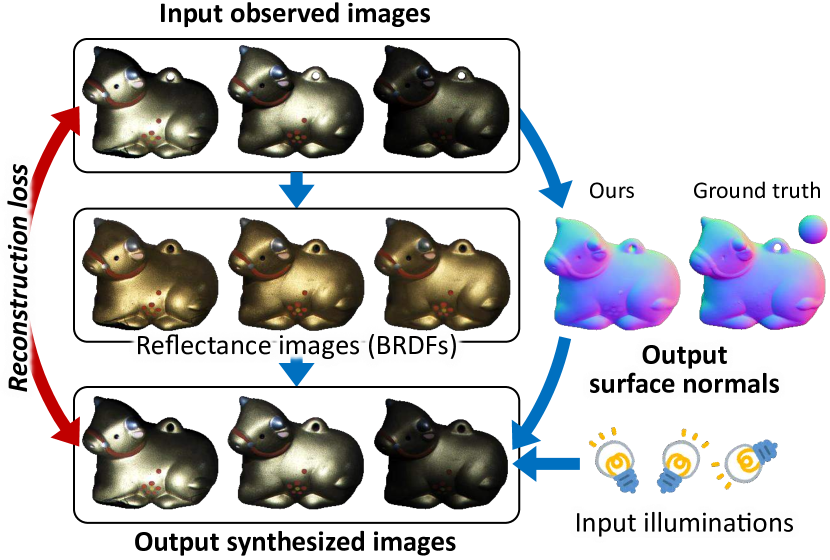
Figure 1: Reconstruction based photometric stereo. Given multiple images observed under varying illuminations, our inverse-rendering network estimates a surface normal map and reflectance images. We then reconstruct (or render) the observed images using these estimates and input illuminations. The synthesized images are used to define reconstruction loss for unsupervised learning.

1 Introduction

3D shape recovery from images is a central problem in computer vision. While geometric approaches such as binocular (Kendall et al., 2017; Taniai et al., 2017) and multi-view stereo (Furukawa & Ponce, 2010) use images from different viewpoints to triangulate 3D points, photometric stereo (Woodham, 1980) uses varying shading cues of multiple images to recover 3D surface normals. It is well known that photometric methods prevail in recovering fine details of surfaces, and play an essential role for highly accurate 3D shape recovery in combined approaches (Nehab et al., 2005; Esteban et al., 2008; Park et al., 2017). Although there exists a closed-form least squares solution to the simplest Lambertian surfaces, such ideally diffuse materials rarely exist in the real word. Photometric stereo for surfaces with unknown general reflectance properties (i.e., bidirectional reflectance distribution functions or BRDFs) still remains as a fundamental challenge (Shi et al., 2018).

Meanwhile, deep learning technologies have drastically pushed the envelope of state-of-the-art in many computer vision tasks such as image recognition (Krizhevsky et al., 2012; He et al., 2015, 2016), segmentation (He et al., 2017b) and stereo vision (Kendall et al., 2017). As for photometric stereo, it is promising to replace hand-crafted reflectance models with deep neural networks to learn complicated BRDFs. However, studies in this direction so far are surprisingly limited (Santo et al., 2017; Hold-Geoffroy et al., 2018). This is possibly due to difficulties of making a large amount of training data with ground truth. Accurately measuring surface normals of real objects is very difficult, because we need highly accurate 3D shapes to reliably compute surface gradients. In fact, a real-world scene benchmark of photometric stereo with ground truth has only recently been introduced by precisely registering laser-scanned 3D meshes onto 2D images (Shi et al., 2018). Using synthetic training data is possible (Santo et al., 2017), but we need photo-realistic rendering that should ideally account for various realistic BRDFs and object shapes, spatially-varying BRDFs and materials, presence of cast shadows and interreflections, etc. This is more demanding than training-data synthesis for stereo and optical flow (Mayer et al., 2016) where rendering by the simplest Lambertian reflectance often suffices. Also, measuring BRDFs of real materials requires efforts and an existing BRDF database (Matusik et al., 2003) provides only a limited number of materials.

As another difficulty of applying deep learning to photometric stereo, when networks are pre-trained, they need to be invariant to permutation of inputs, i.e., permuting input images (and corresponding illuminations) should not change the resulting surface normals. Existing neural network methods (Santo et al., 2017) avoid this problem by assuming the same illumination patterns throughout training and testing phases, which limits application scenarios of methods.

In this paper, we propose a novel convolutional neural network (CNN) architecture for general BRDF photometric stereo. Given observed images and corresponding lighting directions, our network inverse renders surface normals and spatially-varying BRDFs from the images, which are further fed into the reflectance (or rendering) equation to synthesize observed images (see Fig. 1). The network weights are optimized by minimizing reconstruction loss between observed and synthesized images, enabling unsupervised learning that does not use ground truth normals. Furthermore, learning is performed directly on a test scene during the testing phase without any pre-training. Therefore, the permutation invariance problem does not matter in our framework. Our method is evaluated on a challenging real-world scene benchmark (Shi et al., 2018) and is shown to outperform state-of-the-art learning-based (Santo et al., 2017) and other classical unsupervised methods (Shi et al., 2014, 2012; Ikehata & Aizawa, 2014; Ikehata et al., 2012; Wu et al., 2010; Goldman et al., 2010; Higo et al., 2010; Alldrin et al., 2008). We summarize the advantages of our method as follows.

• Existing neural network methods require pre-training using synthetic data, whenever illumination conditions of test scenes change from the trained ones. In contrast, our physics-based approach can directly fit network weights for a test scene in an unsupervised fashion.

• Compared to classical physics-based approaches, we leverage deep neural networks to learn complicated reflectance models, rather than manually analyzing and inventing reflectance properties and models.

• Yet, our physics-based network architecture allows us to exploit prior knowledge about reflectance properties that have been broadly studied in the literature.

2 Preliminaries

Before presenting our method, we recap basic settings and approaches in photometric stereo. Suppose a reflective surface with a unit normal vector $\bar{\bm{n}}\in\mathbb{R}^{3}$ is illuminated by a point light source $\bm{\ell}\in\mathbb{R}^{3}$ (where $\bm{\ell}=\ell\cdot\bar{\bm{\ell}}$ has an intensity $\ell>0$ and a unit direction $\bar{\bm{\ell}}$), without interreflection and ambient lighting. When this surface is observed by a linear-response camera in a view direction $\bar{\bm{v}}\in\mathbb{R}^{3}$, its pixel intensity $I\in\mathbb{R}_{+}$ is determined as follows.

$$I=s\rho(\bar{\bm{n}},\bar{\bm{\ell}},\bar{\bm{v}})\max(\bm{\ell}^{T}\bar{\bm{n}},0)$$ (1)

Here, $s\in\{0,1\}$ is a binary function for the presence of a cast shadow, $\rho(\bar{\bm{n}},\bar{\bm{\ell}},\bar{\bm{v}})$ is a BRDF, and $\max(\cdot,0)$ represents an attached shadow. Figure 2 illustrates this situation.

The goal of photometric stereo is to recover the surface normal $\bar{\bm{n}}$ from intensities $I$, when changing illuminations $\bm{\ell}$. Here, we usually assume a camera with a fixed viewpoint and an orthogonal projection model, in which case the view direction $\bar{\bm{v}}$ is constant and typically $\bar{\bm{v}}=(0,0,1)^{T}$. Also, light sources are assume to be infinitely distant so that $\bm{\ell}$ is uniform over the entire object surfaces.

Figure 2: Surface reflectance and BRDFs. We illustrate a situation where an object surface point with a normal vector $\bar{\bm{n}}$ is illuminated by an infinitely distant point light source in a direction $\bar{\bm{\ell}}$, and is observed by a camera in a view direction $\bar{\bm{v}}$. Unknown BRDFs have major components of diffuse and specular reflections. Shadows occur at surfaces where $\bar{\bm{\ell}}^{T}\bar{\bm{n}}\leq 0$ (attached shadow) or the light ray is occluded by objects (cast shadow).

2.1 Lambertian model and least squares method

When the BRDF $\rho(\bar{\bm{n}},\bar{\bm{\ell}},\bar{\bm{v}})$ is constant as $\rho_{0}$, the surface is purely diffuse. Such a model is called the Lambertian reflectance and the value $\rho_{0}$ is called albedo. In this case, estimation of $\bar{\bm{n}}$ is relatively easy, because for bright pixels ($I>0$) the reflectance equation of Eq. (1) becomes a linear equation: $I=\bm{\ell}^{T}\bm{n}$ where $\bm{n}=\rho_{0}\bar{\bm{n}}$. Therefore, if we know at least three intensity measurements $\bm{I}\in\mathbb{R}^{M}_{+}$ ($M\geq 3$) and their lighting conditions $\bm{L}=[\bm{\ell}_{1},\bm{\ell}_{2},\ldots,\bm{\ell}_{M}]^{T}\in\mathbb{R}^{M\times 3}$, then we obtain a linear system

$$\bm{I}=\bm{L}\bm{n},$$ (2)

which is solved by least squares as

$$\bm{n}=\bm{L}^{\dagger}\bm{I}.$$ (3)

Here, $\bm{L}^{\dagger}$ is the pseudo inverse of $\bm{L}$, and the resulting vector $\bm{n}=\rho_{0}\bar{\bm{n}}$ is then L2-normalized to obtain the unit normal $\bar{\bm{n}}$.

In practice, images are contaminated as $\bm{I}+\bm{e}$ due to sensor noises, interreflections, etc. Therefore, we often set a threshold $\tau$ for selecting inlier observation pixels $I_{i}>\tau$.

When the lighting conditions $\bm{L}$ are unknown, the problem is called uncalibrated photometric stereo. It is known that the problem has the so-called bas-relief ambiguity (Belhumeur et al., 1999), and is difficult even for the Lambertian surfaces. In this paper, we focus on the calibrated photometric stereo settings that assume known lighting conditions.

2.2 Photometric stereo for general BRDF surfaces

When the BRDF $\rho(\bar{\bm{n}},\bar{\bm{\ell}},\bar{\bm{v}})$ has unknown non-Lambertian properties, photometric stereo becomes very challenging, because we essentially need to know the form of the BRDF $\rho(\bar{\bm{n}},\bar{\bm{\ell}},\bar{\bm{v}})$ by assuming some reflectance model to it or by directly estimating $\rho(\bar{\bm{n}},\bar{\bm{\ell}},\bar{\bm{v}})$ along with the surface normal $\bar{\bm{n}}$. Below we briefly review existing such approaches and their limitations. For more comprehensive reviews, please refer to a recent excellent survey by Shi et al. (2018).

Ourlier rejection based methods.

A group of methods treat non-Lambertian reflectance components including specular highlights and shadows as outliers to the Lambertian model. Thus, Eq. (2) is rewritten to

$$\bm{I}=\bm{L}\bm{n}+\bm{e},$$ (4)

where non-Gaussian outliers $\bm{e}$ are assume to be sparse. Recent methods solve this sparse regression problem by using robust statistical techniques (Wu et al., 2010; Ikehata et al., 2012) or using learnable optimization networks (Xin et al., 2016; He et al., 2017a). However, this approach cannot handle broad and soft specularity due to the collapse of the sparse outlier assumption (Shi et al., 2018).

Analytic BRDF models.

Another type of methods use more realistic BRDF models than the Lambertian model matured in the computer graphics literature, e.g., the Torrance-Sparrow model (Georghiades, 2003), the Ward model (Chung & Jia, 2008), or a Ward mixture model (Goldman et al., 2010). These models explicitly consider specularity rather than treating it as outliers, and often take a form of the sum of diffuse and specular components as follows.

$$\rho(\bar{\bm{n}},\bar{\bm{\ell}},\bar{\bm{v}})=\rho_{\text{diff}}+\rho_{\text{spec}}(\bar{\bm{n}},\bar{\bm{\ell}},\bar{\bm{v}})$$ (5)

However, these methods rely on hand-crafted models that can only handle narrow classes of materials.

General isotropic BRDF properties.

More advanced methods directly estimate the unknown BRDF $\rho(\bar{\bm{n}},\bar{\bm{\ell}},\bar{\bm{v}})$ by exploiting some general BRDF properties. For example, many materials have an isotopic BRDF that only depends on relative angles between $\bar{\bm{n}}$, $\bar{\bm{\ell}}$ and $\bar{\bm{v}}$. Given the isotropy, Ikehata & Aizawa (2014) further assume the following bi-variate BRDF function

$$\rho(\bar{\bm{n}},\bar{\bm{\ell}},\bar{\bm{v}})=\rho(\bar{\bm{n}}^{T}\bar{\bm{\ell}},\bar{\bm{\ell}}^{T}\bar{\bm{v}})$$ (6)

with monotonicity and non-negativity constraints. Similarly, Shi et al. (2014) exploit a low-frequency prior of BRDFs and propose a bi-polynomial BRDF:

$$\rho(\bar{\bm{n}},\bar{\bm{\ell}},\bar{\bm{v}})=\sum_{i=0}^{k}\sum_{j=0}^{k}C_{ij}x^{i}y^{j},$$ (7)

where $x=\bar{\bm{n}}^{T}\bar{\bm{h}}$, $y=\bar{\bm{\ell}}^{T}\bar{\bm{h}}$, and $\bar{\bm{h}}=(\bar{\bm{\ell}}+\bar{\bm{v}})/\|\bar{\bm{\ell}}+\bar{\bm{v}}\|_{2}$.

Our method is close to the last approach in that we learn broad classes of a BRDF from observations without restricting it to a particular reflectance model. However, unlike those methods that fully rely on careful human analysis of BRDF properties, we leverage the powerful expressibility of deep neural networks to learn general complicated BRDFs. Yet, our network architecture also explicitly uses the physical reflectance equation of Eq. (1) internally, which allows us to incorporate abundant wisdom about reflectance developed in the literature, into neural network based approaches.

Figure 3: Proposed network architecture for photometric stereo. We use two subnetworks, both are fully convolutional. [Top] The photometric stereo network (PSNet) outputs a surface normal map $\bar{\bm{N}}$ as the desired solution, given an image tensor $\bm{I}$ that concatenates all observed images $\{\bm{I}_{1},\bm{I}_{2},\ldots,\bm{I}_{M}\}$ of a test scene. [Bottom] The image reconstruction network (IRNet) synthesizes each observed image $\bm{I}_{i}$ using the rendering equation. IRNet is used to define reconstruction loss between the observed and synthesized images for unsupervised learning. Note that, as calibrated photometric stereo, the lighting directions $\{\bm{\ell}_{1},\bm{\ell}_{2},\ldots,\bm{\ell}_{M}\}$ are also provided as inputs, and used for the computations of the rendering equation and a specular component input $\bm{S}_{i}$. Also, dimensionality $B\times D\times H\times W$ of tensors denotes a minibatch size $B$, channel number $D$, and spatial resolution $H\times W$, respectively, where $B=1$ is omitted in PSNet.

3 Proposed method

In this section, we present our novel inverse-rendering based neural network architecture for photometric stereo, and explain its learning procedures with a technique of early-stage weak supervision. Here, as standard settings of calibrated photometric stereo, we assume $M$ patterns of light source directions $\bm{\ell}_{i}$ ($i\in\{1,2,\ldots,M\}$) and corresponding image observations $\bm{I}_{i}$ as inputs. We also assume that the mask $\bm{O}$ of target object regions is provided. Our goal is to estimate the surface normal map $\bar{\bm{N}}$ of the target object regions.

Notations.

We use bold capital letters for tensors and matrices, and bold small letters for vectors. We use tensors of dimensionality $D\times H\times W$ to represent images, and normal and other feature maps, where $D$ is some channel number and $H\times W$ is the spatial resolution. Thus, $\bm{I}_{i}\in\mathbb{R}^{C\times H\times W}$ and $\bar{\bm{N}}\in\mathbb{R}^{3\times H\times W}$, where $C$ is the number of color channels of images. We use the subscript $p$ to denote a pixel location of such tensors, e.g., $\bar{\bm{N}}_{p}\in\mathbb{R}^{3}$ is a normal vector at $p$. The light vectors $\bm{\ell}_{i}$ can also have color channels, in which case $\bm{\ell}_{i}\in\mathbb{R}^{3\times C}$ are matrices but we use a small letter for intuitiveness. The index $i$ is always used to denote the observation index $i\in\{1,2,\ldots,M\}$. When we use tensors of dimensionality $B\times D\times H\times W$, the first dimension $B$ denotes a minibatch size processed in one SGD iteration.

3.1 Network architecture

We illustrate our network architecture in Fig. 3. Our method uses two subnetworks, which we name the photometric stereo network (PSNet) and image reconstruction network (IRNet), respectively. PSNet predicts a surface normal map as the desired output, given the input images. On the other hand, IRNet synthesizes observed images using the rendering equation of Eq. (1). The synthesized images are used to define reconstruction loss with the observed images, which produces gradients flowing into both networks and enables learning without ground truth supervision. We now explain these two networks in more details below.

3.1.1 Photometric stereo network

Given a tensor $\bm{I}\in\mathbb{R}^{MC\times H\times W}$ that concatenates all $M$ input images along the channel axis, PSNet first converts it to an abstract feature map $\bm{\Phi}\in\mathbb{R}^{D_{\text{ps}}\times H\times W}$ as

$$\bm{\Phi}=f_{\text{ps1}}(\bm{I};\bm{\theta}_{\text{ps1}}),$$ (8)

and then outputs a surface normal map $\bar{\bm{N}}$ given $\bm{\Phi}$ as

$$\bar{\bm{N}}=f_{\text{ps2}}(\bm{\Phi};\bm{\theta}_{\text{ps2}}).$$ (9)

Here, $f_{\text{ps1}}$ is a feed-forward CNN of three layers with learnable parameters $\bm{\theta}_{\text{ps1}}$, where each layer applies $3$x$3$ Conv of $D_{\text{ps}}$ channels, BatchNorm (Ioffe & Szegedy, 2015), and ReLU. We use channels of $D_{\text{ps}}=384$, and use no skip-connections or pooling. Similarly, $f_{\text{ps2}}$ applies $3$x$3$ Conv and L2 normalization that makes each $\bar{\bm{N}}_{p}$ a unit vector.

3.1.2 Image reconstruction network

IRNet synthesizes each observed image $\bm{I}_{i}$ as $\hat{\bm{I}}_{i}$ based on the rendering equation of Eq. (1). Specifically, IRNet first predicts $R=s\rho(\bar{\bm{n}},\bar{\bm{\ell}},\bar{\bm{v}})$, the multiplication of a cast shadow and a BRDF, under a particular illumination $\bm{\ell}_{i}$ as

$$\hat{\bm{R}}_{i}=f_{\text{ir}}(\bm{I}_{i},\bar{\bm{N}},\bar{\bm{\ell}}_{i},\bar{\bm{v}},\bm{\Phi};\bm{\theta}_{\text{ir}}).$$ (10)

Here, we call $\hat{\bm{R}}_{i}\in\mathbb{R}^{C\times H\times W}$ a reflectance image, which is produced by a CNN $f_{\text{ir}}$ as explained later. Then, IRNet synthesizes each image $\hat{\bm{I}}_{i}$ by the rendering equation below.

$$\hat{\bm{I}}_{i}=\hat{\bm{R}}_{i}\odot\max(\bm{\ell}^{T}_{i}\bar{\bm{N}},\bm{0})$$ (11)

Here, the inner products between light $\bm{\ell}_{i}$ and normal vectors $\bar{\bm{N}}$ are computed at each pixel $p$ by $\bm{\ell}^{T}_{i}\bar{\bm{N}}_{p}$. Note that when $\bm{\ell}_{i}$ has color channels, we multiply a matrix $\bm{\ell}_{i}^{T}\in\mathbb{R}^{C\times 3}$ to $\bar{\bm{N}}_{p}$. Consequently, $\bm{\ell}^{T}_{i}\bar{\bm{N}}$ and $\hat{\bm{R}}_{i}$ have the same dimensions with $\bm{I}$. The $\max(\cdot,\bm{0})$ is done elementwise and is implemented by ReLU, and $\odot$ is elementwise multiplication. We now explain details of $f_{\text{ir}}$ by dividing it into three parts.

Individual observation transform.

The first part transforms each observed image $\bm{I}_{i}$ (which we denote as $\bm{X}_{i}$) into a feature map $\bm{Y}_{i}\in\mathbb{R}^{D_{\text{ir}}\times H\times W}$ as follows.

$$\bm{Y}_{i}=f_{\text{ir1}}(\bm{X}_{i};\bm{\theta}_{\text{ir1}})$$ (12)

The network architecture of $f_{\text{ir1}}$ is the same with $f_{\text{ps1}}$ in Eq. (8), except that we use channels of $D_{\text{ir}}=16$ for $f_{\text{ir1}}$. To more effectively learn BRDFs, we use an additional specularity channel $\bm{S}_{i}$ for the input $\bm{X}_{i}$ as

$$\bm{X}_{i}=\text{Concat}(\bm{I}_{i},\bm{S}_{i}),$$ (13)

where $\bm{S}_{i}\in\mathbb{R}^{1\times H\times W}$ is computed at each pixel $p$ as

$$\bm{S}_{ip}=\bar{\bm{v}}^{T}\bar{\bm{s}}_{ip}=\bar{\bm{v}}^{T}\left[2(\bar{\bm{\ell}}^{T}_{i}\bar{\bm{N}}_{p})\bar{\bm{N}}_{p}-\bar{\bm{\ell}}_{i}\right].$$ (14)

Here, $\bar{\bm{s}}_{ip}$ is the direction of the specular reflection (dashed line between $\bar{\bm{n}}$ and $\bar{\bm{v}}$ in Fig. 2). It is well known by past studies that $\bm{S}_{ip}$ is highly correlated with the actual specular component of a BRDF. Therefore, directly giving it as a hint to the network will promote learning of complex BRDFs.

Global observation blending.

Because $\bm{Y}_{i}$ has limited observation information under a particular illumination $\bm{\ell}_{i}$, we enrich it by $\bm{\Phi}$ in Eq. (8) that has more comprehensive information of the scene. We do this similarly to global and local feature blending in (Charles et al., 2017; Iizuka et al., 2016) as

$$\bm{Z}_{i}=f_{\text{ir2}}(\text{Concat}(\bm{Y}_{i},\bm{\Phi});\bm{\theta}_{\text{ir2}}),$$ (15)

where $f_{\text{ir2}}$ applies $1$x$1$ Conv, BatchNorm, and ReLU. Note that applying Conv to $\text{Concat}(\bm{Y}_{i},\bm{\Phi})$ is efficiently done as $\bm{W}_{1}\bm{Y}_{i}+\bm{W}_{2}\bm{\Phi}+\bm{b}$ where Conv of $\bm{W}_{2}\bm{\Phi}+\bm{b}$ is computed only once and reused for all observations $i$.

Output.

After the blending, we finally output $\hat{\bm{R}}_{i}$ by

$$\hat{\bm{R}}_{i}=f_{\text{ir3}}(\bm{Z}_{i};\bm{\theta}_{\text{ir3}}),$$ (16)

where $f_{\text{ir3}}$ is 3x3 Conv, BatchNorm, ReLU, and 3x3 Conv. As explained in Eq. (11), the resulting $\hat{\bm{R}}_{i}$ is used to reconstruct each image as $\hat{\bm{I}}_{i}$, which is the final output of IRNet.

Note that the internal channels of IRNet are all the same as $D_{\text{ir}}$. Also, IRNet simultaneously reconstructs all images during SGD iterations, by treating them as a minibatch: $\hat{\bm{I}}=\text{Batch}(\hat{\bm{I}}_{1},\hat{\bm{I}}_{2},\ldots,\hat{\bm{I}}_{M})\in\mathbb{R}^{M\times C\times H\times W}$. This learning procedure is more explained in the next section.

3.2 Learning procedures (optimization)

We optimize the network parameters $\bm{\theta}$ by minimizing the following loss function using SGD.

$$L=L_{\text{rec}}(\hat{\bm{I}},\bm{I})+\lambda_{t}L_{\text{prior}}(\bar{\bm{N}},\bar{\bm{N}}^{\prime})$$ (17)

The first term defines reconstruction loss between the synthesized $\hat{\bm{I}}$ and observed images $\bm{I}$, which is explained in Sec. 3.2.1. The second term defines weak supervision loss between the predicted $\bar{\bm{N}}$ and some prior normal map $\bar{\bm{N}}^{\prime}$. This term is only activated in early iterations of SGD (i.e., $\lambda_{t}=0$ when $t>T$) in order to warm up randomly initialized networks and stabilize the learning. This is more explained in Sec. 3.2.2. Other implementation details and hyper-parameter settings are described in Sec. 3.2.3.

Most importantly, the network is directly fit for a particular test scene without any pre-training on other data, by updating the network parameters $\bm{\theta}$ over SGD iterations. Final results are obtained at convergence.

3.2.1 Reconstruction loss

The reconstruction loss is defined as mean absolute errors between $\hat{\bm{I}}$ and $\bm{I}$ over target object regions $\bm{O}$ as

$$L_{\text{rec}}(\hat{\bm{I}},\bm{I})=\frac{1}{MCO}\sum_{i,c,p}\bm{O}_{p}|\hat{\bm{I}}_{icp}-{\bm{I}_{icp}}|.$$ (18)

Here, $\bm{O}$ in $\{1,0\}^{1\times H\times W}$ is the binary object mask, and $O=\sum_{p}\bm{O}_{p}$ is its object area size. Using absolute errors increases the robustness to high-intensity specular highlights.

3.2.2 Early-stage weak supervision

If the target scene has relatively simple reflectance properties, the reconstruction loss alone can often lead to a good solution, even starting with randomly initialized networks. However, for complex scenes, we need to warm up the network by adding the following weak supervision.

$$\lambda_{t}L_{\text{prior}}(\bar{\bm{N}},\bar{\bm{N}}^{\prime})=\lambda_{t}\frac{1}{O}\sum_{p}\bm{O}_{p}\|\bar{\bm{N}}_{p}-{\bar{\bm{N}}^{\prime}_{p}}\|_{2}^{2}$$ (19)

Here, the prior normal map $\bar{\bm{N}}^{\prime}$ is obtained by the simplest least squares method described in Sec. 2.1 using all observed pixels without any thresholding. Due to the presence of shadows and non-Lambertian specularity, this least squares solution can be very inaccurate. However, even such priors work well in our method, because we only use them to guide the optimization in its early stage. For this, we set $\lambda_{t}$ to $0.1c$ for initial 50 iterations, and then set it to zero afterwards. The coefficient $c$ is to adaptively balance weights between $L_{\text{rec}}$ and $L_{\text{prior}}$, and is computed as the mean intensities of $\bm{I}$ over target object regions, i.e., $c=L_{\text{rec}}(\bm{0},\bm{I})$.

3.2.3 Implementation details

We use Adam (Kingma & Ba, 2015) as the optimizer. For each test scene, we iterate SGD updates for $1000$ steps. Adam’s hyper-parameter $\alpha$ is set to $\alpha_{0}=8\times 10^{-4}$ for first 900 iterations, and then decreased to $\alpha_{0}/10$ for last 100 iterations for fine-tuning. We use the default values for the other hyper-parameters. The convolution weights are randomly initialized by He initialization (He et al., 2015).

In each iteration, PSNet predicts a surface normal map $\bar{\bm{N}}$, and then IRNet reconstructs all observed images $\hat{\bm{I}}$ as samples of a minibatch. Given $\bar{\bm{N}}$ and $\hat{\bm{I}}$, we compute the loss $L$ and update the parameters $\bm{\theta}$ of both networks.

When computing the reconstruction loss $L_{\text{rec}}$ in Eq. (18), we randomly dropout 90% of its elements and rescale $L_{\text{rec}}$ by a factor of 10 instead. This treatment is to compensate for the well known issue of poor local convergence of SGD by the use of a large minibatch (Keskar et al., 2017).

Because we learn network parameters during testing, we always run BatchNorm by the training mode using statistics of given data (i.e., we never use moving-average statistics).

Before being fed into the network, the input images $\bm{I}$ are cropped by a loose bounding box of the target object regions for reducing redundant computations. Then, the images are normalized by global scaling as

$$\bm{I}^{\prime}=\bm{I}/(2\sigma),$$ (20)

where $\sigma$ is the square-root of mean squared intensities of $\bm{I}$ over target regions. For PSNet, the normalized image tensor $\bm{I}^{\prime}$ is further concatenated with the binary mask $\bm{O}$ as input.

Table 1: Comparisons on ten real-world scenes of the DiLiGenT photometric stereo benchmark (Shi et al., 2018). We compare our proposed method with ten existing calibrated photometric stereo methods. Here, we show mean angular errors in degrees (i.e., the mean of $\arccos(\bar{\bm{N}}^{T}_{p}\bar{\bm{N}}^{\star}_{p})$ over the object regions using ground truth normals $\bar{\bm{N}}^{\star}_{p}$) for ten scenes, and average scores. Our method achieves best accuracies for all except two scenes of goblet and harvest. The second best method (Santo et al., 2017) also uses a deep neural network, but it requires supervised pre-training on synthetic data and outperforms the other existing methods only for harvest. The results of the baseline least squares method are used in our method as prior normals for weak supervision. Since the priors are used only for an early-stage of learning, their low accuracies are not critical to the performance of our method. Note that, due to a non-deterministic property of our method, its accuracy for each scene is evaluated as the median score of 11 rounds run.

Observed &

synthesized images

Ground truth /

Reconstruction errors

Ours

Santo et al. (2017)

Shi et al. (2014)

Baseline

(least squares)

reading (intensity $\times 10$) 11.03 15.51 13.63 19.80

harvest (intensity $\times 10$) 22.59 16.86 25.44 30.62

Figure 4: Visual comparisons for reading and harvest scenes. From left to right columns in each scene, we show 1) observed and our synthesized images, 2) ground truth normal and image reconstruction error maps, and 3–6) estimated surface normal and angular error maps by four methods. Numbers under angular error maps show their mean errors. See the supplementary material for more comparisons.

Table 2: Evaluations of the proposed network architecture and weak supervision. For each item we show median and mean scores (in left and right) by 11 rounds run. Here, S, G and WS denote the specularity input, global observation blending, and weak supervision by a prior normal map, respectively. Cell colors of red/blue indicate worse/better relative accuracy compared to the proposed settings.

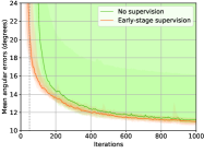
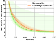
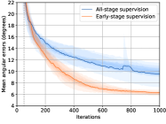
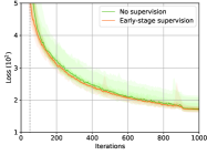
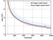
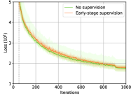
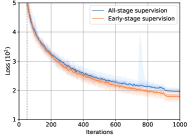
reading (early-stage vs. no/all-stage supervision)

cow (early-stage vs. no/all-stage supervision)

Figure 5: Convergence analysis with different types of weak supervision. We show learning curves of mean angular errors (top) and loss values (bottom) for reading and cow, profiled by distributions of 11 rounds run (colored region) and medians (solid line). Compared to the proposed early-stage supervision (red), using no/all-stage supervision (green/blue) is often unstable or inaccurate. Vertical lines at $t=50$ indicate termination of early-stage supervision. See the supplementary material for results of other scenes. Best viewed in color.

4 Experiments

In this section we evaluate our method using a challenging real-world scene benchmark called DiLiGenT (Shi et al., 2018). In Sec. 4.1, we show comparisons with state-of-the-art photometric stereo methods. We then more analyze our network architecture in Sec. 4.2 and weak supervision technique in Sec. 4.3. In the experiments, we use $M=96$ of observed images for each scene provided by the DiLiGenT dataset. Our method is implemented in Chainer (Tokui et al., 2015) and is run on a single nVidia Tesla V100 GPU with 16 GB memory and 32 bit floating-point precision.

4.1 Real-world scene benchmark (DiLiGenT)

We show our results on the DiLiGenT benchmark (Shi et al., 2018) in Table 4, where we compare our method with ten existing methods by mean angular errors. We also show visual comparisons of the top three and baseline methods for reading and harvest in Fig. 4. Our method achieves the best average score and best individual scores for eight scenes (excepting only two scenes of goblet and harvest) that contain various materials and reflectance surfaces. This is remarkable considering that another neural network method (Santo et al., 2017) outperforms the other existing methods only for harvest, in spite of its supervised learning. This harvest is the most difficult scene of all due to heavy interactions of cast shows and interreflections as well as spatially-varying materials and complex metallic BRDFs. For such complex scenes, supervised pre-training (Santo et al., 2017) is effective. The baseline method poorly performs especially for specular objects. Although we use its results as guidance priors, its low accuracy is not critical to our method thanks to the proposed early-stage supervision. We more analyze it in Sec. 4.3.

4.2 Analysis of the network architecture

In the middle part of Table 2, we show performance changes of our method by modifying its architecture. Specifically, we test two settings where we disable two connections from PSNet to IRNet, i.e., the specularity channel input and the global observation blending described in Sec. 3.1.2. As shown, the proposed full architecture performs best, while the removal of the specularity channel input has the most negative impact. As expected, directly inputting a specularity channel indeed eases learning of complex BRDFs (e.g., metallic surfaces in cow), demonstrating a strength of our physics-based network architecture that can exploit known pysical reflectance properties for BRDF learning.

4.3 Effects of early-stage weak supervision

We here evaluate the effectiveness of our learning strategy using early-stage weak supervision, by comparing with two cases where we use no or all-stage supervision (i.e., $\lambda_{t}$ is $0$ or constant). See the bottom part of Table 2 for performance comparisons. Learning with no supervision produces comparable median scores but worse mean scores, compared to early-stage supervision. This indicates that learning with no supervision is very unstable and often gets stuck at bad local minimums, as shown in Fig. 5 (green profiles). On the other hand, learning with all-stage supervision is relatively stable but is strongly biased by inaccurate least-squares priors, often producing worse solutions as shown in Fig. 5 (blue profiles). In contrast, learning with the proposed early-stage supervision (red profiles) is more stable and persistently continues to improve accuracy even after terminating the supervision at $t=50$ (shown as vertical dashed lines).

5 Discussions and related work

Our method is inspired by recent work of deep image prior by Ulyanov et al. (2018). They show that architectures of CNNs themselves behave as good regularizers for natural images, and show successful results for unsupervised tasks such as image super-resolution and inpainting by fitting a CNN for a single test image. However, their simple glass-hour network does not directly apply to photometric stereo, because we here need to simultaneously consider surface normal estimation that accounts for global statistics of observations, as well as reconstruction of individual observations for defining the loss. Our novel architecture addresses this problem by resorting to ideas of classical physics-based approaches to photometric stereo.

Our network architecture is also partly influenced by that of (Santo et al., 2017), which regresses per-pixel observations $\bm{I}_{p}\in\mathbb{R}^{M}$ to a 3D normal vector using a simple feed-forward network of five fully-connected and ReLU layers plus an output layer. Our PSNet becomes similar to theirs, if we use 1x1 Conv with more layers and channels (i.e., they use channels of $4096$ and $2048$ for the five internal layers). Since our method only needs to learn reflectance properties of a single test scene, our PSNet requires fewer layers and channels. More importantly, we additionally introduce IRNet, which allows direct unsupervised learning on test data.

There are some other early studies on photometric stereo using (shallow) neural networks. These methods work under more restricted conditions, e.g., assuming pre-training by a calibration sphere of the same material with target objects (Iwahori et al., 1993, 1995), special image capturing setups (Iwahori et al., 2002; Ding et al., 2009), or the Lambertian surfaces (Cheng, 2006; Elizondo et al., 2008), whereas none of them is required by our method.

Currently, our method has limitations of a slow running time (e.g., 1 hour to do 1000 SGD iterations for each scene) and limited performances to complex scenes (e.g., harvest). However, several studies (Akiba et al., 2017; You et al., 2017; Goyal et al., 2017) show fast training of CNNs using extremely large minibatches and tuned scheduling of SGD step-sizes. Since our dense prediction method can use at most a large minibatch of $M\times H\times W$ pixel samples, the use of such acceleration schemes may improve the convergence speed. Also, a pre-training approach similar to (Santo et al., 2017) is still feasible for our method, which will accelerate the convergence and will also increase accuracy to complex scenes (with the loss of permutation invariance). Thorough analyses in such directions are left as our future work.

6 Conclusions

In this paper, we have presented a novel CNN architecture for photometric stereo. The proposed unsupervised learning approach bridges a gap between existing supervised neural network methods and many other classical physics-based unsupervised methods. Consequently, our method can learn complicated BRDFs by leveraging both powerful expressibility of deep neural networks and physical reflectance properties known by past studies, achieving the state-of-the-art performance in an unsupervised fashion just like classical methods. We also hope that our idea of physics-based unsupervised learning stimulates further research on tasks that lack of ground truth data for training, because even so the physics is everywhere in the real world, which will provide strong clues for the hidden data we desire.

¹ RIKEN AIP, Nihonbashi, Tokyo, Japan

In this supplementary material, we provide results for all the ten benchmark scenes that are omitted in the paper due to the page limitation. Specifically, we provide the following additional results.

• Visual comparisons of our method and existing methods.

• Our image reconstruction results.

• Convergence analyses of our method by different types of weak supervision.

A Additional visual comparisons

In Figures A1–A10, we show surface normal estimates and their angular error maps for all ten scenes from the DiLiGenT dataset, comparing our method with three methods by Santo et al. (2017), Shi et al. (2014), and Ikehata & Aizawa (2014), and also the baseline least squares method. Here, the best result for each scene is obtained by either of the top four methods (where 8 of 10 best results are by our method), whose mean angular error is shown by a bold font number.

B Additional image reconstruction results

In Figures A11–A20, we show our image reconstruction results for all ten scenes from the DiLiGenT dataset. For each scene we show 6 images from 96 observed images, and for each observed image we show our synthesized image, intermediate reflectance image, and reconstruction error map. Here, the reflectance images represent multiplication of spatially-varying BRDFs and cast shadows under a particular illumination condition. We can clearly see cast shadows in reflectance images appearing in the results of bear and buddha. Note that for better visualization, the image intensities are scaled by a factor of $255/2$ after the proposed global scaling normalization.

C Additional convergence analyses

In Figures A21–A30, we show convergence analyses for all ten scenes from the DiLiGenT dataset, where the proposed early-stage supervision is compared with no and all-stage supervision. Training without supervision is very unstable, while training with all-stage supervision is strongly biased by inaccurate least square priors. Note that for better comparison, the median profiles of the proposed early-stage weak supervision (red solid lines) are overlayed in the plots of no and all-stage supervision.

Ground truth /
Observed image

Ours

Santo et al. (2017)

Shi et al. (2014)

Ikehata & Aizawa (2014)

Baseline
(least squares)

ball

1.47

2.02

1.74

3.34

4.10

Figure A1: Visual comparisons for ball scene. From left to right columns, we show 1) the ground truth normal map and an observed image, 2) our normal estimate and its error map, 3–6) four pairs of a normal estimate and its error map by three state-of-the-art methods (Santo et al., 2017; Shi et al., 2014; Ikehata & Aizawa, 2014) and the baseline least squares method.

Ground truth /
Observed image

Ours

Santo et al. (2017)

Shi et al. (2014)

Ikehata & Aizawa (2014)

Baseline
(least squares)

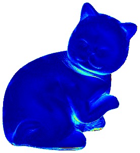
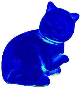
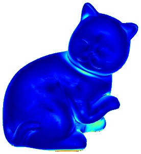
cat

5.44

6.54

6.12

6.74

8.41

Figure A2: Visual comparisons for cat scene. See also explanations in Fig. A1.

Ground truth /
Observed image

Ours

Santo et al. (2017)

Shi et al. (2014)

Ikehata & Aizawa (2014)

Baseline
(least squares)

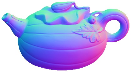
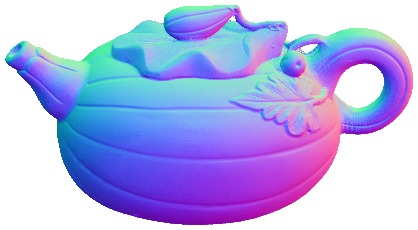
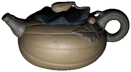
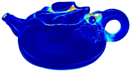
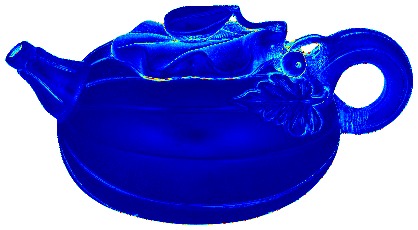
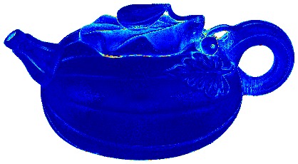
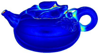
pot1

6.09

7.05

6.51

6.64

8.89

Figure A3: Visual comparisons for pot1 scene. See also explanations in Fig. A1.

Ground truth /
Observed image

Ours

Santo et al. (2017)

Shi et al. (2014)

Ikehata & Aizawa (2014)

Baseline
(least squares)

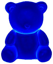
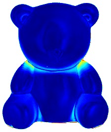
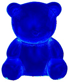
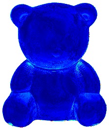
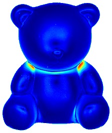
bear

5.79

6.31

6.12

7.11

8.39

Figure A4: Visual comparisons for bear scene. See also explanations in Fig. A1.

Ground truth /
Observed image

Ours

Santo et al. (2017)

Shi et al. (2014)

Ikehata & Aizawa (2014)

Baseline
(least squares)

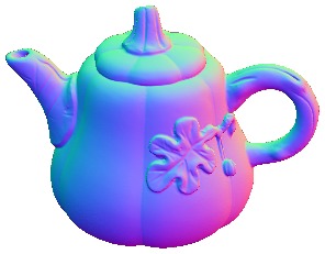
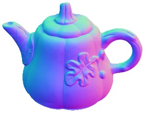
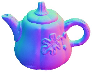
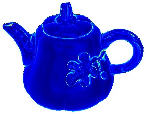
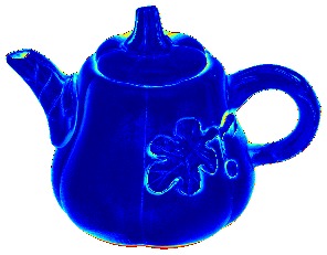
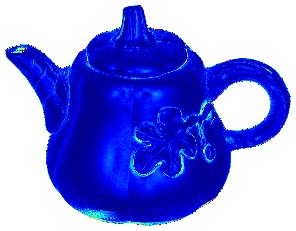
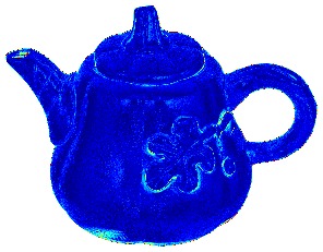
pot2

7.76

7.86

8.78

8.77

14.65

Figure A5: Visual comparisons for pot2 scene. See also explanations in Fig. A1.

Ground truth /
Observed image

Ours

Santo et al. (2017)

Shi et al. (2014)

Ikehata & Aizawa (2014)

Baseline
(least squares)

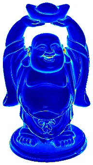
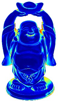
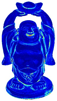
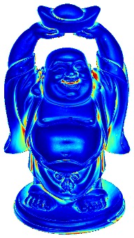
buddha

10.36

12.68

10.60

10.47

14.92

Figure A6: Visual comparisons for buddha scene. See also explanations in Fig. A1.

Ground truth /
Observed image

Ours

Santo et al. (2017)

Shi et al. (2014)

Ikehata & Aizawa (2014)

Baseline
(least squares)

goblet

11.47

11.28

10.09

9.71

18.5

Figure A7: Visual comparisons for goblet scene. See also explanations in Fig. A1.

Ground truth /
Observed image

Ours

Santo et al. (2017)

Shi et al. (2014)

Ikehata & Aizawa (2014)

Baseline
(least squares)

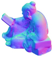
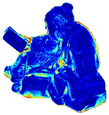
reading

11.03

15.51

13.63

14.19

19.80

Figure A8: Visual comparisons for reading scene. See also explanations in Fig. A1.

Ground truth /
Observed image

Ours

Santo et al. (2017)

Shi et al. (2014)

Ikehata & Aizawa (2014)

Baseline
(least squares)

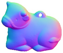
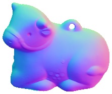
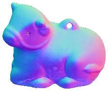
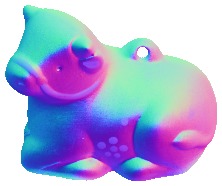
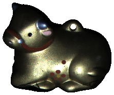
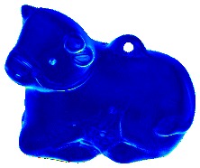
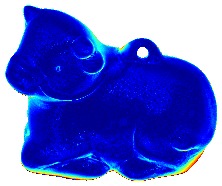
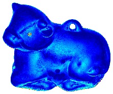
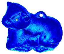
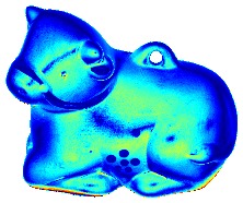
cow

6.32

8.01

13.93

13.05

25.60

Figure A9: Visual comparisons for cow scene. See also explanations in Fig. A1.

Ground truth /
Observed image

Ours

Santo et al. (2017)

Shi et al. (2014)

Ikehata & Aizawa (2014)

Baseline
(least squares)

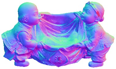
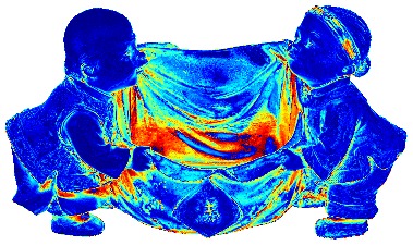
harvest

22.59

16.86

25.44

25.95

30.62

Figure A10: Visual comparisons for harvest scene. See also explanations in Fig. A1.

Figure A11: Our image reconstruction results for ball scene. We show our image reconstruction results for six selected images. From top to bottom, we show observed images, our synthesized images, our reflectance images, and reconstruction errors between observed and synthesized images. The error maps show absolute intensity differences scaled by a factor of 10.

Figure A12: Our image reconstruction results for cat scene. See also explanations in Fig. A11.

Figure A13: Our image reconstruction results for pot1 scene. See also explanations in Fig. A11.

Figure A14: Our image reconstruction results for bear scene. See also explanations in Fig. A11.

Figure A15: Our image reconstruction results for pot2 scene. See also explanations in Fig. A11.

Figure A16: Our image reconstruction results for buddha scene. See also explanations in Fig. A11.

Figure A17: Our image reconstruction results for goblet scene. See also explanations in Fig. A11.

Figure A18: Our image reconstruction results for reading scene. See also explanations in Fig. A11.

Figure A19: Our image reconstruction results for cow scene. See also explanations in Fig. A11.

Figure A20: Our image reconstruction results for harvest scene. See also explanations in Fig. A11.

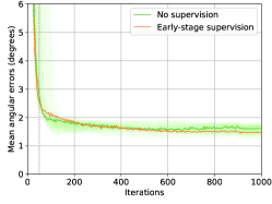
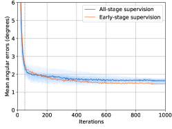
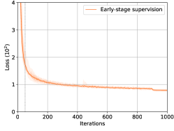
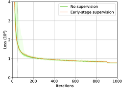
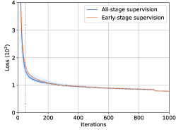
Early-stage supervision

No supervision

All-stage supervision

Figure A21: Convergence analysis with different types of weak supervision for ball scene. We compare training curves by using the proposed early-stage supervision (left) with no supervision (middle), and all-stage supervision (left). For each case, profiles of mean angular errors and loss values are shown in top and bottom, respectively, which are visualized by distributions of 11 rounds run (colored region) and medians (solid line). Vertical lines at $t=50$ show termination of early-stage supervision.

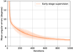
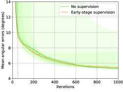
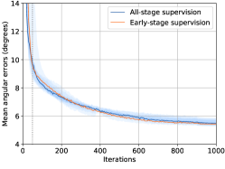
Early-stage supervision

No supervision

All-stage supervision

Figure A22: Convergence analysis with different types of weak supervision for cat scene. See also explanations in Fig. A21.

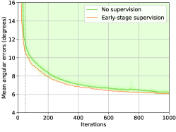
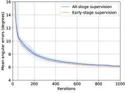
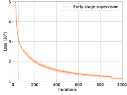
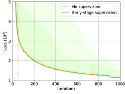
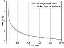
Early-stage supervision

No supervision

All-stage supervision

Figure A23: Convergence analysis with different types of weak supervision for pot1 scene. See also explanations in Fig. A21.

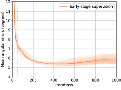
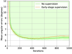
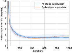
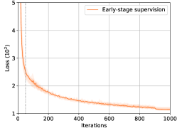
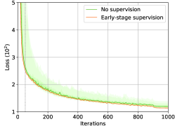
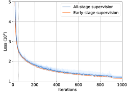
Early-stage supervision

No supervision

All-stage supervision

Figure A24: Convergence analysis with different types of weak supervision for bear scene. See also explanations in Fig. A21.

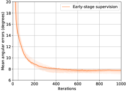
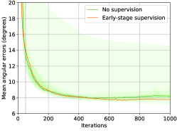
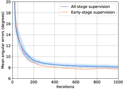
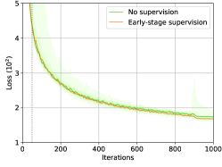
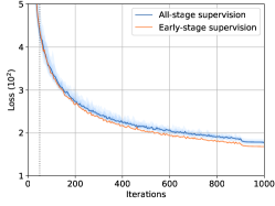
Early-stage supervision

No supervision

All-stage supervision

Figure A25: Convergence analysis with different types of weak supervision for pot2 scene. See also explanations in Fig. A21.

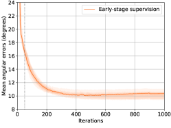
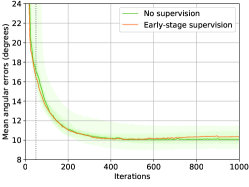
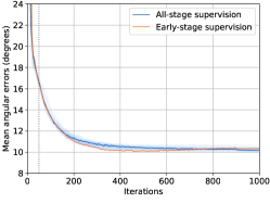
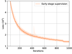
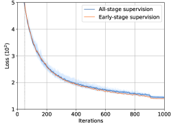
Early-stage supervision

No supervision

All-stage supervision

Figure A26: Convergence analysis with different types of weak supervision for buddha scene. See also explanations in Fig. A21.

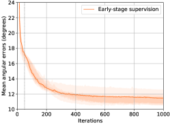
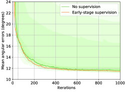
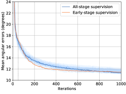
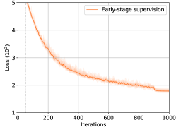
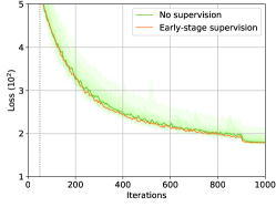
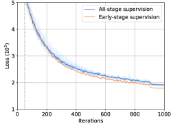
Early-stage supervision

No supervision

All-stage supervision

Figure A27: Convergence analysis with different types of weak supervision for goblet scene. See also explanations in Fig. A21.

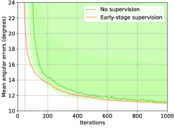
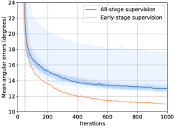
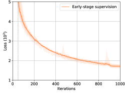
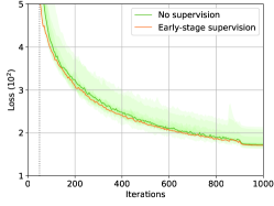
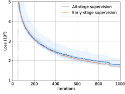
Early-stage supervision

No supervision

All-stage supervision

Figure A28: Convergence analysis with different types of weak supervision for reading scene. See also explanations in Fig. A21.

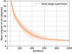
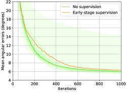
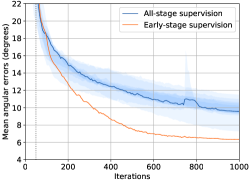
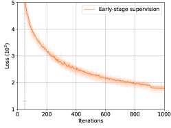
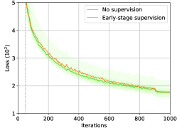
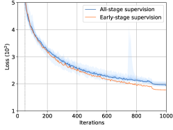
Early-stage supervision

No supervision

All-stage supervision

Figure A29: Convergence analysis with different types of weak supervision for cow scene. See also explanations in Fig. A21.

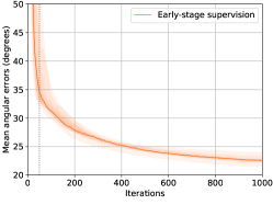
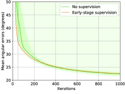
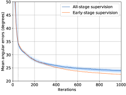
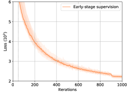
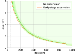
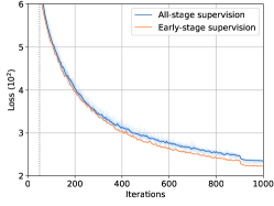
Early-stage supervision

No supervision

All-stage supervision

Figure A30: Convergence analysis with different types of weak supervision for harvest scene. See also explanations in Fig. A21.

References

- Akiba et al. (2017) Akiba, T., Suzuki, S., and Fukuda, K. Extremely Large Minibatch SGD: Training ResNet-50 on ImageNet in 15 Minutes. CoRR, abs/1711.04325, 2017.
- Alldrin et al. (2008) Alldrin, N., Zickler, T., and Kriegman, D. Photometric stereo with non-parametric and spatially-varying reflectance. In Proc. IEEE Conf. Comput. Vis. and Pattern Recognit. (CVPR), 2008.
- Belhumeur et al. (1999) Belhumeur, P. N., Kriegman, D. J., and Yuille, A. L. The Bas-Relief Ambiguity. Int’l J. Comput. Vis. (IJCV), 35(1):33–44, Nov 1999.
- Charles et al. (2017) Charles, R. Q., Su, H., Kaichun, M., and Guibas, L. J. PointNet: Deep Learning on Point Sets for 3D Classification and Segmentation. In Proc. IEEE Conf. Comput. Vis. and Pattern Recognit. (CVPR), pp. 77–85, 2017.
- Cheng (2006) Cheng, W.-C. Neural-network-based photometric stereo for 3d surface reconstruction. In Proc. IEEE Int’l Joint Conf. Neural Network, pp. 404–410, 2006.
- Chung & Jia (2008) Chung, H.-S. and Jia, J. Efficient photometric stereo on glossy surfaces with wide specular lobes. In Proc. IEEE Conf. Comput. Vis. and Pattern Recognit. (CVPR), 2008.
- Ding et al. (2009) Ding, Y., Iwahori, Y., Nakamura, T., Woodham, R. J., He, L., and Itoh, H. Self-calibration and Image Rendering Using RBF Neural Network. In Proc. Int’l Conf. Knowledge-Based and Intell. Inf. and Engin. Syst., pp. 705–712, 2009.
- Elizondo et al. (2008) Elizondo, D., Zhou, S.-M., and Chrysostomou, C. Surface Reconstruction Techniques Using Neural Networks to Recover Noisy 3D Scenes. In Proc. Int’l Conf. Artificial Neural Networks, pp. 857–866, 2008.
- Esteban et al. (2008) Esteban, C. H., Vogiatzis, G., and Cipolla, R. Multiview photometric stereo. IEEE Trans. Pattern Anal. Mach. Intell. (TPAMI), 30(3):548–554, 2008.
- Furukawa & Ponce (2010) Furukawa, Y. and Ponce, J. Accurate, Dense, and Robust Multiview Stereopsis. IEEE Trans. Pattern Anal. Mach. Intell. (TPAMI), 32(8):1362–1376, 2010.
- Georghiades (2003) Georghiades, A. S. Incorporating the Torrance and Sparrow model of reflectance in uncalibrated photometric stereo. In Proc. Int’l Conf. Comput. Vis. (ICCV), pp. 816–823, 2003.
- Goldman et al. (2010) Goldman, D. B., Curless, B., Hertzmann, A., and Seitz, S. M. Shape and Spatially-Varying BRDFs from Photometric Stereo. IEEE Trans. Pattern Anal. Mach. Intell. (TPAMI), 32(6):1060–1071, 2010.
- Goyal et al. (2017) Goyal, P., Dollár, P., Girshick, R. B., Noordhuis, P., Wesolowski, L., Kyrola, A., Tulloch, A., Jia, Y., and He, K. Accurate, Large Minibatch SGD: Training ImageNet in 1 Hour. CoRR, abs/1706.02677, 2017.
- He et al. (2017a) He, H., Xin, B., Ikehata, S., and Wipf, D. P. From Bayesian Sparsity to Gated Recurrent Nets. In Adv. Neural Inf. Process. Syst. (NIPS), pp. 5560–5570. 2017a.
- He et al. (2015) He, K., Zhang, X., Ren, S., and Sun, J. Delving Deep into Rectifiers: Surpassing Human-Level Performance on ImageNet Classification. In Proc. Int’l Conf. Comput. Vis. (ICCV), pp. 1026–1034, 2015.
- He et al. (2016) He, K., Zhang, X., Ren, S., and Sun, J. Deep residual learning for image recognition. In Proc. IEEE Conf. Comput. Vis. and Pattern Recognit. (CVPR), pp. 770–778, 2016.
- He et al. (2017b) He, K., Gkioxari, G., Dollár, P., and Girshick, R. Mask R-CNN. In Proc. Int’l Conf. Comput. Vis. (ICCV), 2017b.
- Higo et al. (2010) Higo, T., Matsushita, Y., and Ikeuchi, K. Consensus photometric stereo. In Proc. IEEE Conf. Comput. Vis. and Pattern Recognit. (CVPR), pp. 1157–1164, 2010.
- Hold-Geoffroy et al. (2018) Hold-Geoffroy, Y., Gotardo, P. F. U., and Lalonde, J. Deep Photometric Stereo on a Sunny Day. CoRR, abs/1803.10850, 2018.
- Iizuka et al. (2016) Iizuka, S., Simo-Serra, E., and Ishikawa, H. Let there be Color!: Joint End-to-end Learning of Global and Local Image Priors for Automatic Image Colorization with Simultaneous Classification. ACM Trans. Graphics (ToG), 35(4):110:1–110:11, 2016.
- Ikehata & Aizawa (2014) Ikehata, S. and Aizawa, K. Photometric Stereo Using Constrained Bivariate Regression for General Isotropic Surfaces. In Proc. IEEE Conf. Comput. Vis. and Pattern Recognit. (CVPR), pp. 2187–2194, 2014.
- Ikehata et al. (2012) Ikehata, S., Wipf, D., Matsushita, Y., and Aizawa, K. Robust photometric stereo using sparse regression. In Proc. IEEE Conf. Comput. Vis. and Pattern Recognit. (CVPR), pp. 318–325, 2012.
- Ioffe & Szegedy (2015) Ioffe, S. and Szegedy, C. Batch Normalization: Accelerating Deep Network Training by Reducing Internal Covariate Shift. In Proc. Int’l Conf. Mach. Learn. (ICML), volume 37, pp. 448–456, 2015.
- Iwahori et al. (1993) Iwahori, Y., Woodham, R. J., Tanaka, H., and Ishii, N. Neural network to reconstruct specular surface shape from its three shading images. In Proc. 1993 Int’l Conf. Neural Networks, volume 2, pp. 1181–1184, 1993.
- Iwahori et al. (1995) Iwahori, Y., Bagheri, A., and Woodham, R. J. Neural network implementation of photometric stereo. In Proc. Vision Interface, 1995.
- Iwahori et al. (2002) Iwahori, Y., Watanabe, Y., Woodham, R. J., and Iwata, A. Self-calibration and neural network implementation of photometric stereo. In Proc. Int’l Conf. Pattern Recognit. (ICPR), volume 4, pp. 359–362, 2002.
- Kendall et al. (2017) Kendall, A., Martirosyan, H., Dasgupta, S., Henry, P., Kennedy, R., Bachrach, A., and Bry, A. End-To-End Learning of Geometry and Context for Deep Stereo Regression. In Proc. Int’l Conf. Comput. Vis. (ICCV), 2017.
- Keskar et al. (2017) Keskar, N. S., Mudigere, D., Nocedal, J., Smelyanskiy, M., and Tang, P. T. P. On Large-Batch Training for Deep Learning: Generalization Gap and Sharp Minima. In Proc. Int’l Conf. Learn. Repres. (ICLR), 2017.
- Kingma & Ba (2015) Kingma, D. P. and Ba, J. Adam: A Method for Stochastic Optimization. In Proc. Int’l Conf. Learn. Repres. (ICLR), 2015.
- Krizhevsky et al. (2012) Krizhevsky, A., Sutskever, I., and Hinton, G. E. ImageNet Classification with Deep Convolutional Neural Networks. In Adv. Neural Inf. Process. Syst. (NIPS), pp. 1097–1105. 2012.
- Matusik et al. (2003) Matusik, W., Pfister, H., Brand, M., and McMillan, L. Efficient Isotropic BRDF Measurement. In Proc. Eurographics Workshop on Rendering, 2003.
- Mayer et al. (2016) Mayer, N., Ilg, E., Häusser, P., Fischer, P., Cremers, D., Dosovitskiy, A., and Brox, T. A Large Dataset to Train Convolutional Networks for Disparity, Optical Flow, and Scene Flow Estimation. In Proc. IEEE Conf. Comput. Vis. and Pattern Recognit. (CVPR), pp. 4040–4048, 2016.
- Nehab et al. (2005) Nehab, D., Rusinkiewicz, S., Davis, J., and Ramamoorthi, R. Efficiently Combining Positions and Normals for Precise 3D Geometry. ACM Trans. Graphics (ToG), 24(3):536–543, 2005.
- Park et al. (2017) Park, J., Sinha, S. N., Matsushita, Y., Tai, Y. W., and Kweon, I. S. Robust Multiview Photometric Stereo using Planar Mesh Parameterization. IEEE Trans. Pattern Anal. Mach. Intell. (TPAMI), 39(8):1591–1604, 2017.
- Santo et al. (2017) Santo, H., Samejima, M., Sugano, Y., Shi, B., and Matsushita, Y. Deep Photometric Stereo Network. In Proc. Int’l Workshop Physics Based Vision meets Deep Learning (PBDL) in ICCV, 2017.
- Shi et al. (2012) Shi, B., Tan, P., Matsushita, Y., and Ikeuchi, K. Elevation Angle from Reflectance Monotonicity: Photometric Stereo for General Isotropic Reflectances. In Proc. Eur. Conf. Comput. Vis. (ECCV), pp. 455–468, 2012.
- Shi et al. (2014) Shi, B., Tan, P., Matsushita, Y., and Ikeuchi, K. Bi-Polynomial Modeling of Low-Frequency Reflectances. IEEE Trans. Pattern Anal. Mach. Intell. (TPAMI), 36(6):1078–1091, 2014.
- Shi et al. (2018) Shi, B., Wu, Z., Mo, Z., Duan, D., Yeung, S.-K., and Tan, P. A Benchmark Dataset and Evaluation for Non-Lambertian and Uncalibrated Photometric Stereo. IEEE Trans. Pattern Anal. Mach. Intell. (TPAMI), 2018. (to appear).
- Taniai et al. (2017) Taniai, T., Matsushita, Y., Sato, Y., and Naemura, T. Continuous 3D Label Stereo Matching using Local Expansion Moves. IEEE Trans. Pattern Anal. Mach. Intell. (TPAMI), 2017. (accepted).
- Tokui et al. (2015) Tokui, S., Oono, K., Hido, S., and Clayton, J. Chainer: a next-generation open source framework for deep learning. In Proc. Workshop Mach. Learn. Syst. (LearningSys) in NIPS, 2015. URL https://chainer.org.
- Ulyanov et al. (2018) Ulyanov, D., Vedaldi, A., and Lempitsky, V. S. Deep Image Prior. In Proc. IEEE Conf. Comput. Vis. and Pattern Recognit. (CVPR), 2018. (to appear).
- Woodham (1980) Woodham, R. J. Photometric method for determining surface orientation from multiple images. Optical Engineering, 19(1):139–144, 1980.
- Wu et al. (2010) Wu, L., Ganesh, A., Shi, B., Matsushita, Y., Wang, Y., and Ma, Y. Robust photometric stereo via low-rank matrix completion and recovery. In Proc. Asian Conf. Comput. Vis. (ACCV), pp. 703–717, 2010.
- Xin et al. (2016) Xin, B., Wang, Y., Gao, W., Wipf, D. P., and Wang, B. Maximal Sparsity with Deep Networks? In Adv. Neural Inf. Process. Syst. (NIPS), pp. 4340–4348. 2016.
- You et al. (2017) You, Y., Zhang, Z., Hsieh, C., and Demmel, J. ImageNet Training in Minutes. CoRR, abs/1709.05011, 2017.