A large sample of shear selected clusters from the Hyper Suprime-Cam Subaru Strategic Program S16A wide field mass maps

Abstract

We present the result of searching for clusters of galaxies based on weak gravitational lensing analysis of the $\sim 160$ deg² area surveyed by Hyper Suprime-Cam (HSC) as a Subaru Strategic Program. HSC is a new prime focus optical imager with a 1.5 diameter field of view on the 8.2-meter Subaru telescope. The superb median seeing on the HSC $i$-band images of $0.56$ arcsec allows the reconstruction of high angular resolution mass maps via weak lensing, which is crucial for the weak lensing cluster search. We identify 65 mass map peaks with signal-to-noise (SN) ratio larger than 4.7, and carefully examine their properties by cross-matching the clusters with optical and X-ray cluster catalogs. We find that all the 39 peaks with SN$>5.1$ have counterparts in the optical cluster catalogs, and only 2 out of the 65 peaks are probably false positives. The upper limits of X-ray luminosities from ROSAT All Sky Survey (RASS) imply the existence of an X-ray under-luminous cluster population. We show that the X-rays from the shear selected clusters can be statistically detected by stacking the RASS images. The inferred average X-ray luminosity is about half that of the X-ray selected clusters of the same mass. The radial profile of the dark matter distribution derived from the stacking analysis is well modeled by the Navarro-Frenk-White profile with a small concentration parameter value of $c_{500}\sim 2.5$, which suggests that the selection bias on the orientation or the internal structure for our shear selected cluster sample is not strong.

1 Introduction

Clusters of galaxies are important tools for testing theories of structure formation and constraining cosmological parameters via the abundance and its evolution. Traditionally, clusters have been identified using their optical or X-ray emission and thus the resulting catalogs are inevitably biased toward the selection of more luminous objects. In the dark matter dominated universe, however, it is challenging to quantify the selection function of such catalogs, given the uncertainty in the connection between dark and luminous objects. Ideally we want to select clusters of galaxies based on their masses, which are the the most critical parameter in characterizing clusters. A mass selected sample of clusters allows more direct and straightforward comparisons with $N$-body simulations, which leads to better understanding of the connection between luminous and dark matter in clusters as well as more direct tests of structure formation theories.

*7l Attempts to search for clusters based on the weak lensing shear Telescope $n_{\rm g}$ Median Seeing Area $n_{\rm peak}$ ($\nu>4.5$) Purity Ref.
[arcmin^-2] [arcsec] [deg²] [deg^-2] [%]
Mayall 19 0.90 7.5 0.27 100 (2$/2$) Wittman et al. (2006)
CFHT 35 0.91 3.6 0.56 100 (2$/$2) Gavazzi & Soucail (2007)
MPG$/$ESO 12 0.90 19 0.89 65 (11$/$17)^∗ Schirmer et al. (2007)
Subaru 46 0.55 2.2 0.95 75 (3$/$4) Miyazaki et al. (2007)
CFHT 11.2 0.71 55.0 0.93 59 (30$/$51) Shan et al. (2012)
Subaru 34.5 0.71 $\sim 3$ 2.3100(7/7)Utsumi et al. (2014)
Subaru 24 0.57 9.0 0.89 100 (8/8) Hamana et al. (2015)
Subaru 20.9 0.58 2.3 3.5 100 (8$/$8) Miyazaki et al. (2015)
^∗only $S$-statistics peaks are considered in this compilation.

Weak gravitational lensing has the potential to offer the most reliable route to select clusters independently of any assumptions about their baryon contents and thermal and dynamical states. This technique uses statistical measures of distorted shapes (“shear”) of faint distance galaxies induced by the tidal gravitational field integrated along the line-of-sight. This, in turn, allows a reconstruction of two-dimensional surface mass density maps (Kaiser & Squires, 1993; Seitz & Schneider, 1995; Schneider, 1996) where we are able to locate the dark matter concentrations from the peak positions. The redshift information can be obtained by correlating the peak location with optically selected cluster catalogs. Because the selection function of the peaks can be defined in a straightforward way (Hamana et al., 2012), such shear-selected cluster catalog is useful for both cluster astrophysics and cosmology. For example, the shear selected cluster sample will complement studies planned by eRosita all sky X-ray cluster surveys through the comparison of the cluster selection functions.

While the weak lensing search of clusters has several advantages as discussed above, it has not been possible to construct a large sample of shear selected clusters due to observational difficulties. First, the demand on the observing facility is high. In order to locate the cluster scale dark matter halo via weak lensing, deep imaging with the limiting magnitude deeper than $i_{\rm AB}\;\sim\;24.5$ is necessary to achieve sufficient number density of source galaxies. At the same time, wide field imaging camera is necessary to search for rare objects like clusters. Satisfying both the depth and wide area for constructing a large sample of shear selected clusters has been difficult in previous imaging surveys. Second, because the lensing kernel is broad along the line-of-sight direction, the two-dimensional lensing signal is affected by small foreground and background structures along the line-of-sight, which may cause “fake” signals that are not associated with single massive objects (White et al., 2002; Hennawi & Spergel, 2005). Such contaminations by projections may reduce the value of shear selected cluster catalogs. For example, Hamana et al. (2004) evaluated the contamination rate of shear selected clusters based on the weak lensing ray-trace simulation and found that the contamination rate can reach up to 42% when one sets the threshold of the signal-to-noise ratio (SN, or $\nu$) to 4. Adopting a higher threshold for SN mitigates such contaminations, although this further reduces the number of shear selected clusters.

Observationally, there have been several attempts to search for clusters via weak lensing (see also Table 1). The Deep Lens Survey is one of the pioneering projects where Wittman et al. (2001) announced the first discovery of a galaxy cluster at $z=0.276$ by weak lensing. Schirmer et al. (2007) identified 17 mass map peaks with $\nu>4.5$ on 19 deg² area imaged by MPG/ESO 2.2-meter telescope where the average galaxy number density is $n_{\rm g}=12~{}{\rm arcmin}^{-2}$ with the median seeing of $0.9$ arcsec. They examined the galaxy over-density on the $R$-band image around the peak ($<2^{\prime}$) and found that 65% of the peaks accompany the galaxy concentrations. The rest of the peaks were most likely artifacts due to the noise because these preferentially appear on the shallower imaging data. When they raised the peak detection threshold up to 6, all the peaks have optical counterparts. Miyazaki et al. (2007) showed that nearly 75% of the peaks ($\nu>4.5$) have optical or X-ray counterparts on a 2.2 deg² field observed by 8.2-meter Subaru with Suprime-Cam under the seeing of $0.55$ arcsec ($n_{\rm g}=46~{}{\rm arcmin}^{-2}$). Even if the detection threshold is decreased down to 4, the purity was kept high, around 80%. This demonstrates that the contamination level can be indeed reduced using deeper and sharper imaging data.

Following these pilot studies, weak lensing mass map peaks have been searched on much wider survey area such as 4-meter CFHT Legacy Survey (CFHTLS). Shan et al. (2012) presented the results from a 51 deg² area ($\sim 30$% of CFHTLS-Wide Survey area, $n_{\rm g}=11.5~{}{\rm arcmin}^{-2}$ with the median seeing of $0.71$ arcsec). They found 51 mass map peaks with $\nu>4.5$, 59% of which have counterparts in the optical cluster catalogs generated using photometric redshifts from the same CFHTLS data set (Thanjavur et al., 2009). Liu et al. (2015) also identified $\sim 40$ mass map peaks with $\nu>4.5$ from $\sim 130$ deg² of CFHT Stripe 82 Survey. There have also been attempts to constrain cosmological parameters from the number counts of peaks, although not necessarily using high $\nu$ peaks (Liu et al., 2015, 2015; Hamana et al., 2015; Kacprzak et al., 2016).

Shear selected cluster catalog can uniquely address the abundance of clusters with anomalously high mass-to-light ratios. The possibility of such dark halos is argued by e.g., Weinberg & Kamionkowski (2002). However, previous shear selected cluster searches mentioned above did not successfully distinguish dim clusters from false positive peaks caused by the noise or the line-of-sight projection of small systems, mainly due to the lower detection thresholds for selecting peaks from mass maps. The lack of follow-up data might also have complicated the cross-correlation of peaks and galaxy concentrations.

This paper presents the first attempt to generate a useful shear selected cluster catalog where the contamination is mitigated by adopting a higher peak detection threshold than what was adopted by previous works and the catalog is validated by comparing with optically selected groups/clusters based on the multi-color deep Hyper Suprime-Cam (HSC) data. HSC realizes seeing limited imaging on Maunakea over the entire 1.5 degree diameter field of view (Miyazaki et al., 2017). Combined with the large aperture of the Subaru telescope, the camera is an ideal facility for weak lensing surveys. Using the commissioning data of HSC over 2.3 deg², Miyazaki et al. (2015) indeed showed that the angular resolution of the weak lensing mass map is fine enough to collect un-contaminated cluster samples over the wide redshift range, $0.2<z<0.7$. In this paper, we extend the previous work to construct a large sample of shear selected clusters from the HSC Subaru Strategic Program (SSP) survey data, which already covered more than 100 deg² with full five broadband colors.

This paper is organized as follows. In Section 2, we describe the HSC-SSP data used for generating weak lensing mass maps. The mass maps are presented in Section 3, and peaks in the mass maps are identified in Section 4. We discuss properties of our sample of shear selected clusters in Section 5, and give conclusion in Section 6. Unless explicitly stated, we adopt a WMAP9 cosmological model with $\Omega_{\rm M}=0.287$, $\Omega_{\Lambda}=0.713$, $\sigma_{8}=0.820$, $H_{0}=100h\;{\rm km}\;{\rm s}^{-1}\;{\rm Mpc^{-1}}$ with $h=0.693$ (Hinshaw et al., 2013).

2 Imaging data set and the shape measurements

The HSC-SSP is a legacy optical imaging survey consisting of three layers; Wide, Deep and UltraDeep. HSC-Wide is designed to be a competitive cosmological survey in which nearly ten times larger survey field is covered with one magnitude deeper imaging compared with the existing CFHTLS. HSC-Deep and -UltraDeep uniquely combine narrow-band imaging with broad-band imaging to explore frontiers of studies in high redshift objects and galaxy evolution. In total 300 nights were awarded for the HSC-SSP. The survey started on March 2014 and will continue for about six years. The details of the HSC-SSP survey is given in Aihara et al. (2017).

In this paper, we adopt the HSC-Wide data from an internal data release called S16A. The integration time of a single exposure is 200 sec in $i$-band. The survey area is covered by the camera’s circular field of view with dithered pointings. The dithering pattern is determined so that any location on the sky is visited by at least six exposures for $i$-band, yielding the total exposure time of 1200 sec. The HSC-Wide $i$-band imaging is preferentially conducted under good seeings, resulting in a median seeing measured over three years of $0.56$ arcsec FWHM (Miyazaki et al., 2017).

The survey fields are mostly located along the equator (S16A field names XMM, GAMA09H, WIDE12H, GAMA15H, and VVDS) except the one (S16A field name HECTOMAP). The total area of the HSC-Wide S16A data used for this work amounts to $\sim 160$ deg².

The data reduction is made with the HSC pipeline (Bosch et al., 2017), which is based on “LSST-Stack” (Ivezić et al., 2008; Axelrod et al., 2010), a software suite being developed for the LSST project. We adopt the re-Gaussianization method (Hirata & Seljak, 2003) for measuring shapes of galaxies. Detail of the Point Spread Function (PSF) corrections, shear measurements, and the results of null tests are shown in Mandelbaum et al. (2017). In this HSC S16A shape catalog, the faint magnitude cut is conservatively chosen to $i<24.5$. With this conservative cut, however, the number density of source galaxies is still high, with a raw number density of $n_{\rm g}=25~{}{\rm arcmin}^{-2}$. Additional systematics tests using weak lensing mass maps for the HSC S16A shape catalog are given in Oguri et al. (2017b), in which small residual systematics in weak lensing mass maps are confirmed. While the mass maps are constructed without applying any cut in photometric redshifts of source galaxies, we adopt mizuki photometric redshift (Tanaka et al., 2017) to select background galaxies behind clusters when we conduct radial profile fitting for individual shear selected clusters. We note that the selection of photometric redshift in Tanaka et al. (2017) does not affect the individual mass estimate compared with the error.

3 Weak lensing mass maps

3.1 Reconstruction of mass maps

In order to locate the position of dark matter concentrations by weak lensing, we generate two-dimensional mass map from the shear catalog. Since the reconstructed mass map is noisy, smoothing is crucial for detecting any structure in the map. A useful statistics is the so-called aperture mass (Schneider, 1996), which uses essentially a smoothed lensing convergence field $\kappa(\boldsymbol{\theta})$ defined as

$$M_{\rm ap}(\boldsymbol{\theta}_{0})=\int d^{2}\theta\;\kappa(\boldsymbol{\theta})U(|\boldsymbol{\theta}-\boldsymbol{\theta}_{0}|),$$ (1)

where $U(\theta)$ is a circular-symmetric filter function. When a compensated filter is chosen, $\int d\theta\theta U(\theta)=0$, the zero point of kappa does not contribute to $M_{\rm ap}$. Using the shear $\gamma$, $M_{\rm ap}$ can be rewritten as

$$M_{\rm ap}(\boldsymbol{\theta}_{0})=\int d^{2}\theta\gamma_{T}(\boldsymbol{\theta},\boldsymbol{\theta}_{0})\;Q(|\boldsymbol{\theta}-\boldsymbol{\theta}_{0}|),$$ (2)

where $\gamma_{T}$ is the tangential shear at the point $\boldsymbol{\theta}$ with respect to the point $\boldsymbol{\theta}_{0}$, and $Q(\theta)$ is related to $U(\theta)$ as

$$Q(\theta)=\frac{2}{\theta^{2}}\int_{0}^{\theta}d\theta^{\prime}\theta^{\prime}U(\theta^{\prime})-U(\theta).$$ (3)

The filter $U(\theta)$ must be chosen carefully depending on the purpose. In order to construct a shear selected cluster sample efficiently, the angular size of the filter has to be roughly the scale radius of massive clusters of interest (Hamana et al., 2004). In order to maximize the signal from mass concentration with NFW (Navarro et al., 1997) profile, it is most efficient to choose the spatial filter that follows the radial convergence profile of the NFW profile (Maturi et al., 2005; Marian & Bernstein, 2006). However, near the center there are many observational uncertainties, including the non-linearity in the shape measurement, the dilution by cluster member galaxies, and the large baryonic effect that modifies the density profile near the center. Thus in practice we want to choose the filter $Q(\theta)$ that suppresses the contribution from the cluster center (i.e., small $|Q(\theta)|$ at $\theta\approx 0$). Also it is useful to consider a compensated filter for $U(\theta)$ in order to minimize the effect of the large-scale structure in selecting clusters from mass map peaks (Marian et al., 2010).

In this paper, we consider a generic form for simplicity, adopting a truncated Gaussian (Hamana et al., 2012)

$$U_{\rm G}(\theta) = \frac{1}{\pi\theta_{s}^{2}}\exp\left({-\frac{\theta^{2}}{\theta_{s}^{2}}}\right)-U_{0}$$ (4)

$$Q_{\rm G}(\theta) = \frac{1}{\pi\theta^{2}}\left[1-\left(1+\frac{\theta^{2}}{\theta_{s}}\right)\exp\left({-\frac{\theta^{2}}{\theta_{s}^{2}}}\right)\right],$$ (5)

for $\theta\leq\theta_{\rm out}$ and $U_{\rm G}(\theta)=Q_{\rm G}(\theta)=0$ for $\theta>\theta_{\rm out}$. The parameter $\theta_{s}$ represents the angular scale of the filter, whereas $U_{0}$ is introduced so as to satisfy the condition $\int d\theta\theta U(\theta)=0$. Then the aperture mass is calculated in the two-dimensional grids over the observed data to yield the $M_{\rm ap}$ map. In practice the integral in equation (2) is replaced by a discrete sum of tangential shears estimated from image ellipticities

$$M_{\rm ap}(\boldsymbol{\theta}_{0})=\frac{1}{\bar{W}(\boldsymbol{\theta}_{0})}\sum_{i}w_{i}\epsilon_{T,i}(\boldsymbol{\theta}_{i},\boldsymbol{\theta}_{0})\;Q(|\boldsymbol{\theta}_{i}-\boldsymbol{\theta}_{0}|),$$ (6)

$$\bar{W}(\boldsymbol{\theta}_{0})=\frac{1}{\pi\theta_{\rm out}^{2}}\sum_{|\boldsymbol{\theta}_{i}-\boldsymbol{\theta}_{0}|<\theta_{\rm out}}(1+m_{i})w_{i},$$ (7)

where $\epsilon_{T,i}(\boldsymbol{\theta}_{i},\boldsymbol{\theta}_{0})$ is the tangential component of the ellipticity of the $i$-th galaxy located at $\boldsymbol{\theta}_{i}$ with respect to the center of the aperture, $\boldsymbol{\theta}_{0}$. The parameter $w_{i}$ is the shear weight and $m_{i}$ is the multiplicative bias for the $i$-th galaxy, both of which are derived in Mandelbaum et al. (2017).

The noise of $M_{\rm ap}(\boldsymbol{\theta}_{0})$ is estimated from the variance of the $M_{\rm ap}$ values where the galaxy orientations are randomized in each realization. When we randomize the rotation angle $\phi_{i}$ uniformly from 0 to 2$\pi$, the variance is calculated by

$$\sigma^{2}(\boldsymbol{\theta}_{0}) = \frac{1}{2\pi}\int_{0}^{2\pi}d\phi_{1}\cdot\cdot\cdot d\phi_{n}M^{2}_{\rm ap}(\boldsymbol{\theta}_{0},\phi_{i})$$ (8)

$$-\frac{1}{2\pi}\left(\int_{0}^{2\pi}d\phi_{1}\cdot\cdot\cdot d\phi_{n}M_{\rm ap}(\boldsymbol{\theta}_{0},\phi_{i})\right)^{2}$$

$$= \frac{1}{2\left\{\bar{W}(\boldsymbol{\theta}_{0})\right\}^{2}}\sum_{i}\left\{w_{i}|\epsilon_{T,i}|Q(|\boldsymbol{\theta}_{i}-\boldsymbol{\theta}_{0}|)\right\}^{2}.$$ (9)

We define the signal-to-noise ratio of $M_{\rm ap}$ at the point $\boldsymbol{\theta}_{0}$ as

$${\nu}(\boldsymbol{\theta}_{0})=\frac{M_{\rm ap}(\boldsymbol{\theta}_{0})}{\sigma(\boldsymbol{\theta}_{0})}.$$ (10)

Throughout the paper, we employ reduced shear estimated from the shape measurements as an approximation of the shear. This makes $\nu$ slightly increased; 2 % and 5 % for $\nu=4.7$ and 9.0 peak, respectively. We also note that the multiplicative bias $m$ does not affect the value of $\nu$ for each grid because it changes both $M_{\rm ap}$ and $\sigma$ in the similar manner. However, it changes the absolute value of $M_{\rm ap}$ and $\sigma$, and therefore changes the cluster mass scale for a given $\nu$.

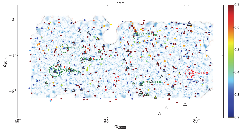
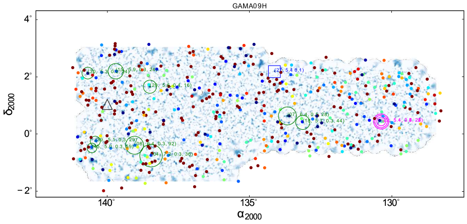
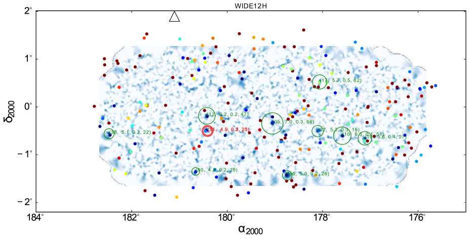
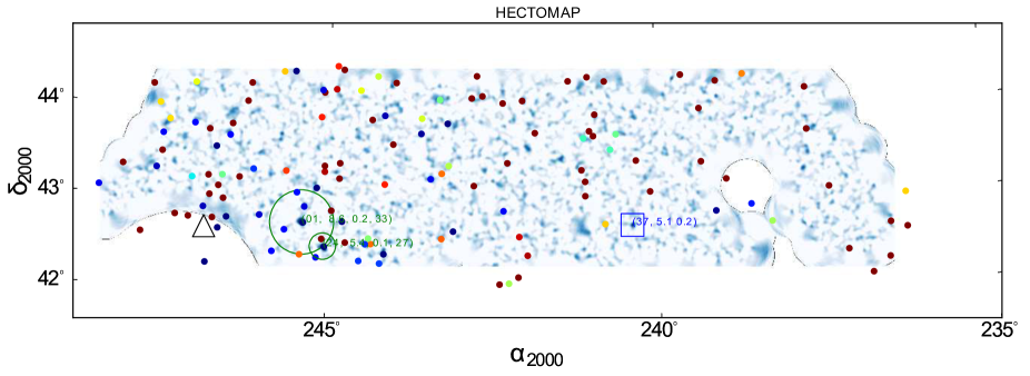
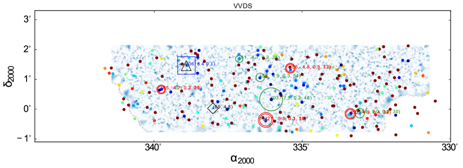
Figures 1, 2, and 3 show the SN map of each field when we adopt the truncated Gaussian filters of $\theta_{s}=1.5^{\prime}$ with the map grid spacing of $0.25^{\prime}$. The filter is truncated at $\theta_{\rm out}=15^{\prime}$. Objects in the shear catalog have various flags such as a bright star flag (Mandelbaum et al., 2017). We eliminate objects with such flags from lensing analysis and this acts as masking of inappropriate field position.

The peaks on the SN map indicates the locations of the mass concentrations of dark matter halos. We recognize the local peaks when three connected pixels on the map exceeds the threshold of $\nu=4.3$. The location of the peak is simply read from the center of the grid whose $\nu$ is maximum. The maximum value is assigned for the SN of that peak.

Based on the discussion made in Section 3.2, we set the peak SN threshold at $\nu=4.7$ in this paper. The number of peaks depends on the choice of the filter scale $\theta_{s}$. We adopted the value that is slightly larger than Hamana et al. (2012), who adopted $\theta_{s}=1^{\prime}$, because in this paper we only consider highly significant peaks whose counterpart clusters tend to be located at relatively low redshift and have larger angular extents. Indeed, the numbers of peaks with the two different filters are 56 and 65 for $\theta_{s}=1^{\prime}$ and $1.5^{\prime}$, respectively. In principle, we can consider multiple mass maps with different filter sizes, which will definitely increase the information content extracted from the mass maps (Marian et al., 2012; Lin et al., 2016), but in this paper we fix the filter size throughout for simplicity.

Figure 1: Weak lensing $M_{\rm ap}$ SN maps for the XMM (upper) and GAMA09H (lower) fields. Small filled circles show the locations of CAMIRA clusters where blue to red color-code corresponds the redshift of 0.2 to 0.7 as is shown in the color bar next to the map of XMM field. Open circles show the locations of the mass map peaks matched with CAMIRA clusters. If multiple CAMIRA clusters are matched with a peak, the number of concentric circle indicate the multiplicity. The first two numbers in brackets show the peak rank and the peak SN. The third numbers and the forth number show the redshift and richness, respectively, but these are not always available. Peaks that do not match with CAMIRA clusters are shown by open squares. Large open triangles indicate MCXC X-ray clusters. Small open triangles show the XXL brightest 100 clusters. Large open diamonds show the location of the peaks that matches neither CAMIRA nor WHL15 clusters.

Figure 2: Same as Figure 1, but weak lensing $M_{\rm ap}$ SN maps of WIDE12H (upper) and GAMA15H (lower) are shown.

Figure 3: Same as Figure 1, but weak lensing $M_{\rm ap}$ SN maps of HECTOMAP (upper) and VVDS (lower) are shown.

3.2 Peaks on the $B$-mode map and the rate of false signals

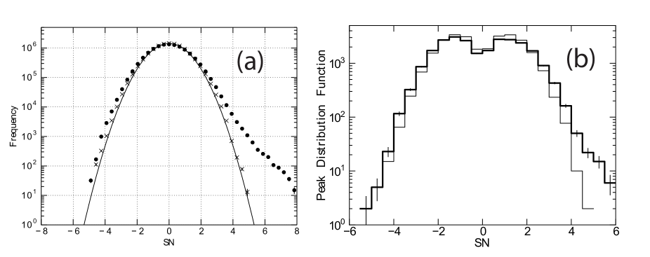
Because the weak lensing is induced by the scalar (gravitational) potential, no $B$-mode signal is generated from lensing in principle. We can use this fact to see whether we have systematic errors in our analysis. $B$-mode SN map can be made from the same galaxy shape catalog where the each galaxy orientation is rotated by 45 degree. In Figure 4 (a), we show the pixel value distribution function of the $B$-mode map as cross symbols ($\times$). As is shown, there is no pixel value beyond $\nu=5$. Solid line shows the Gaussian distribution with $\sigma=1$ with the amplitude normalized to the $B$-mode pixel frequency at $\nu=0$, which nicely agrees with the distribution of the observed $B$-mode distribution. This suggests that $B$-mode map is a Gaussian random field and is not significantly affected by systematic errors. This result, together with the analyses presented in Mandelbaum et al. (2017) and Oguri et al. (2017b), suggests that systematic errors on the $E$-mode mass maps are also not significant and highly significant peaks ($\nu>5$) on the $E$-mode maps are not likely to be generated by the noise or systematic errors. The numbers of less significant peaks on $E$-mode and $B$-mode map are 22 and 4, respectively. Therefore, up to $\sim 20$% of such less significant $E$-mode peaks can be false signals caused by the noise.

Figure 4 (b) shows a local peak height (and trough depth for negative SN) distribution function. Here the local peak (trough) is identified by pixels on the maps whose pixel value are higher (lower) than any values in the surrounding eight pixels This is another representation of the nature of the maps and can be directly compared with the theoretical calculation (Jain & van Waerbeke, 2000). We see significant excess of the peak counts over noise estimated by B-mode peak counts. We could also see the small excess of trough over the noise at SN $<$ 4.5.

Figure 4: (a) Pixel distributions of the $E$-mode ($\bullet$) and $B$-mode ($\times$) $M_{\rm ap}$ SN maps. Error bars of the data are shown which are only visible at $|\rm{SN}|>4$. $B$-mode distribution nicely follows the Gaussian distribution with $\sigma=1$. (b) Local peak distribution function of the same maps. Local peaks on the E-mode maps is shown by thick histogram whereas peaks on B-mode maps by thin histogram.

4 Identifications of the peaks

llrrllllll List of shear selected clusters
rank SN ($\nu$) RA2000 DEC2000 d $z_{\rm cl}$ $N_{\rm mem}$ $M_{500}$ $c_{500}$ Note
[deg] [deg] [$h^{-1}$Mpc] $\times 10^{14}h^{-1}$M_⊙
1 8.62 245.3800 42.7656 0.13 0.152 33.0 2.02$\pm$ 0.41 7.4$\pm$ 4.6 Abell 2183 (z=0.1365) (W)
2 7.52 37.9254 -4.8803 0.05 0.186 116.4 2.72$\pm$ 0.48 2.9$\pm$ 1.1 Abell 0362 (z=0.1843) (W)
3 7.47 336.0460 0.3360 0.11 0.154 48.9 1.83$\pm$ 0.39 7.5$\pm$ 5.2 (W)
4 7.25 138.4610 -0.7610 0.25 0.284 36.1 2.96$\pm$ 0.69 2.1$\pm$ 1.0 (W)
5 7.02 179.0520 -0.3463 0.33 0.254 66.2 3.43$\pm$ 0.67 1.5$\pm$ 0.6 (W)
6 6.41 338.9120 1.4802 – 0.057^† – 1.73$\pm$ 0.43 1.6$\pm$ 0.8 Abell 2457 (z=0.0594) (W)
7 6.40 133.6610 0.6372 0.50 0.121 28.3 1.21$\pm$ 0.31 10.0$\pm$ 0.0 (W)
8 6.39 139.0430 -0.3948 0.33 0.318 92.3 2.96$\pm$ 0.81 4.3$\pm$ 2.5 Abell 0776 (z=0.3359) (W)
9 6.36 37.3951 -3.6099 0.11 0.312 57.0 4.16$\pm$ 0.86 1.3$\pm$ 0.5 (W)
10 6.30 177.5860 -0.6043 0.08 0.135 51.9 1.51$\pm$ 0.33 4.5$\pm$ 2.6 (W)
11 6.20 221.0390 0.1773 – 0.294^† – 3.38$\pm$ 0.75 1.4$\pm$ 0.6 (W)
12 6.17 180.4270 -0.1880 0.16 0.164 48.0 1.69$\pm$ 0.45 1.5$\pm$ 0.8 Abell 1445 (z=0.1694)
13 5.99 30.4210 -5.0203 0.93 0.809 24.0 – –
0.12 0.206 15.4 – –
14 5.99 216.7760 0.7232 0.04 0.296 25.8 2.66$\pm$ 0.63 1.5$\pm$ 0.7 (W)
15 5.95 139.7060 2.2068 0.41 0.298 24.2 2.71$\pm$ 0.61 5.6$\pm$ 3.5 (W)
16 5.77 33.3622 -2.9150 0.40 0.150 34.7 1.29$\pm$ 0.42 2.1$\pm$ 1.5 (W)
17 5.74 178.0610 0.5243 0.23 0.472 62.3 3.50$\pm$ 0.99 7.2$\pm$ 5.2 (W)
18 5.71 133.1200 0.4081 0.40 0.270 44.3 1.92$\pm$ 0.48 10.0$\pm$ 0.0 (W)
19 5.64 177.1120 -0.6583 1.21 0.420 28.0 2.41$\pm$ 0.89 1.5$\pm$ 1.2
20 5.55 138.5050 1.6646 1.48 0.380 16.9 3.67$\pm$ 1.09 1.9$\pm$ 1.3 (W)
21 5.45 336.2300 -0.3638 0.18 0.140 19.2 – –
0.17 0.307 33.8 – –
22 5.43 130.3710 0.4399 1.43 0.454 25.8 – –
0.85 0.215 24.9 – –
0.12 0.413 22.0 – –
23 5.42 213.8900 -0.0515 – – – – –
24 5.39 245.0570 42.5066 0.16 0.142 27.9 2.17$\pm$ 0.83 0.4$\pm$ 0.2 (W)
25 5.37 219.2130 -0.7013 0.80 0.198 18.3 0.88$\pm$ 0.28 10.0$\pm$ 0.0 (W)
26 5.37 213.7780 -0.4879 0.08 0.144 43.0 1.97$\pm$ 0.67 0.4$\pm$ 0.2 Abell 1882 (z=0.1367) (W)
27 5.35 134.1180 2.1991 – 0.126^† – 0.00$\pm$ 0.00 0.0$\pm$ 0.0 (W)
28 5.33 38.1165 -4.7920 0.96 0.276 33.7 1.68$\pm$ 0.51 2.5$\pm$ 1.8 (W)
29 5.33 30.3810 -5.5104 – 0.194^† – 1.36$\pm$ 0.37 10.0$\pm$ 0.0 (W)
30 5.32 140.6830 2.1374 0.07 0.194 24.7 1.15$\pm$ 0.33 10.0$\pm$ 0.0 (W)
31 5.31 219.4300 -0.3264 0.68 0.147 51.3 1.98$\pm$ 0.56 1.1$\pm$ 0.6 (W)
32 5.27 178.1020 -0.5087 0.64 0.311 15.7 2.46$\pm$ 0.77 1.2$\pm$ 0.7 (W)
33 5.22 215.0660 0.9680 0.84 0.168 16.6 – –
0.45 0.515 46.3 – –
0.19 0.322 16.2 – –
34 5.22 223.0820 0.1644 0.18 0.592 53.8 9.59$\pm$ 2.29 1.7$\pm$ 0.7 (W)
35 5.17 211.9870 -0.4783 0.48 0.469 35.9 3.62$\pm$ 1.18 1.4$\pm$ 0.9 (W)
36 5.14 36.3804 -4.2540 0.15 0.155 18.2 1.21$\pm$ 0.34 3.7$\pm$ 2.7
37 5.13 240.3980 42.7484 – 0.223^† – 1.98$\pm$ 0.47 8.0$\pm$ 5.7 (W)
38 5.08 182.4740 -0.5622 0.39 0.178 22.4 1.64$\pm$ 0.56 4.8$\pm$ 4.6 (W)
39 5.07 140.4190 -0.2530 0.56 0.310 29.7 3.08$\pm$ 1.10 0.7$\pm$ 0.4 (W)
40 5.06 216.8680 -0.2016 – – – – –
41 5.05 212.9210 0.4053 0.33 0.252 27.1 – –
0.15 0.148 17.5 – –
42 5.04 223.0940 -0.9723 0.07 0.304 39.0 2.56$\pm$ 0.65 6.9$\pm$ 5.5 (W)
43 5.03 37.6634 -4.9982 0.11 0.272 33.1 1.72$\pm$ 0.66 1.4$\pm$ 1.0 (W)
44 5.02 333.0540 -0.1345 0.14 0.350 30.5 3.04$\pm$ 0.88 1.5$\pm$ 0.9 (W)
45 5.00 140.5350 -0.4895 0.52 0.305 59.4 4.10$\pm$ 1.32 1.0$\pm$ 0.6 (W)
46 5.00 178.7400 -1.4377 0.14 0.158 26.5 2.67$\pm$ 0.86 3.0$\pm$ 3.2 (W)
47 5.00 217.6800 0.8108 0.78 0.149 15.8 – –
0.14 0.312 36.9 – –
48 4.98 220.7900 1.0509 0.33 0.529 45.8 7.30$\pm$ 2.06 1.5$\pm$ 0.8 (W)
49 4.92 223.4620 -1.1209 – 0.277^† – 1.72$\pm$ 0.46 10.0$\pm$ 0.0 (W)
50 4.92 333.3700 -0.1554 1.18 0.357 34.1 – –
0.15 0.100 22.6 – –
51 4.91 180.4100 -0.5046 0.77 0.322 25.3 – –
0.37 0.162 23.9 – –
52 4.90 336.4170 1.0777 0.31 0.281 54.4 1.74$\pm$ 0.59 2.2$\pm$ 1.6 (W)
53 4.88 220.3950 -0.9047 1.34 0.884 16.7 – –
0.24 0.534 56.7 – –
54 4.87 213.6040 -0.3631 0.33 0.144 68.8 1.69$\pm$ 0.68 0.2$\pm$ 0.1 (W)
55 4.84 224.2570 -1.0034 – 0.393^† – 2.78$\pm$ 0.91 9.4$\pm$11.1 (W)
56 4.83 335.4000 1.3859 1.08 0.790 23.4 – –
0.94 0.324 17.6 – –
57 4.82 221.3300 0.1107 0.09 0.287 34.4 2.27$\pm$ 0.66 1.3$\pm$ 0.7 (W)
58 4.78 33.1330 -5.5513 0.97 0.287 64.6 1.84$\pm$ 0.81 0.7$\pm$ 0.5
59 4.77 338.0160 0.0277 – – – – –
60 4.75 180.6600 -1.3542 0.14 0.246 29.7 1.44$\pm$ 0.48 5.2$\pm$ 5.0 (W)
61 4.73 337.1260 1.7066 0.09 0.338 36.0 2.58$\pm$ 0.62 10.0$\pm$ 0.0 (W)
62 4.73 216.6510 0.7982 – 0.592^† – 7.17$\pm$ 2.71 0.4$\pm$ 0.2 (W)
63 4.71 33.4748 -2.8818 1.17 0.288 22.3 1.28$\pm$ 0.53 2.1$\pm$ 2.0
64 4.71 220.5860 0.3355 0.23 0.172 19.2 0.95$\pm$ 0.29 10.0$\pm$ 0.0 (W)
65 4.70 339.7630 0.6681 0.74 0.200 19.2 – –
0.26 0.264 21.3 – –

In total we identify 65 peaks with $\nu>4.7$ for the smoothing size $\theta_{s}=1.5^{\prime}$, which are summarized in Table 4. The peaks are sorted by $\nu$ and we call the order ’rank’. We now compare the peaks with optical and X-ray cluster catalogs.

4.1 Optical counterparts

Based on the same HSC-SSP multi-color photometric data used in this paper, Oguri et al. (2017a) generated an optical cluster catalog using the “Cluster finding algorithm based on Multi-band Identification of Red-sequence gAlaxies” (CAMIRA), which was developed in Oguri (2014). CAMIRA makes use of the stellar population synthesis (SPS) model of Bruzual & Charlot (2003) to compute SEDs of red-sequence galaxies, estimates the likelihood of them being cluster member galaxies for each redshift using $\chi^{2}$ of the SED fitting, constructs a three-dimensional richness map using a compensated spatial filter, and identifies cluster candidates from peaks of the richness map. The richness threshold is set to $N_{\rm mem}=15$ in identifying the clusters.

The locations of the CAMIRA clusters are overlaid on Figures 1, 2, and 3, as small filled circles. Clusters are searched around the peaks with the a loose matching tolerance of $6^{\prime}$ at first. Next, we calculated the comoving distance between the peak and the cluster center using the estimated cluster redshift. The cluster center is the position of the brightest cluster galaxy, BCG, recognized through the CAMIRA algorithm. Then, we identify the peak with the cluster when the distance is within $1.5h^{-1}$Mpc. In some cases, multiple clusters are matched with a peak where cares must be taken because the weak lensing mass estimate is complicated for such peaks.

In Table 4, we list the coordinates of the detected peaks sorted by the SN together with the CAMIRA redshift, $z_{\rm cl}$, the richness, $N_{\rm mem}$, and the distance, $d$, between the peak and the cluster location. Open circles on Figures 1, 2, and 3 show the locations of the peaks matched with a single CAMIRA cluster. When multiple clusters are matched, the multiplicity is indicated by the number of concentric open circles. The diameter of the circle roughly reflect the rank of the cluster such that highly ranked peaks have larger circles. Table 1 summarizes the multiplicity of the matching.

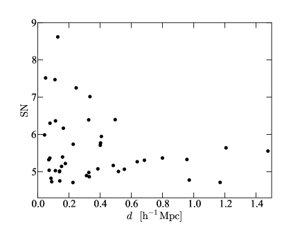
The angular resolution of the weak lensing mass map is usually poorer than that of X-ray map and therefore, the peak position could not be the best proxy for the real dark matter halo center. However, the offset between the real center and our detected peak cannot largely exceed 1.5 arcmin because we adopted the smoothing scale of 1.5 arcmin. The simulation study done by Dietrich et al. (2012) also shows that the offset between the peak position and dark matter halo center is usually smaller than 1 arcmin. On the other hand, the cluster center (the BCG position) is known to have larger scatter up to $1h^{-1}$Mpc with respect to the X-ray center as is shown in Fig.12 of Oguri et al. (2017a). Therefore, in this work, we adopt the peak position as an approximate position of dark matter halo center because not all of X-ray data are in hand. Figure 5 shows the distance between the peak and the cluster center versus SN of the peak where the larger scatters is observed for less significant peaks. This might suggest that the physical association of the peak with the clusters is unlikely whose separation is as large as $1.5h^{-1}$ Mpc although we are not certain how large the actual scatter of BCG position is in CAMIRA catalog.

Figure 5: The distance between the peak position and the cluster center (BCG position) of CAMIRA clusters.

We have 11 peaks which have no counterpart in the CAMIRA cluster catalog. What is the nature of these peaks? We search for the counterparts in a cluster catalogs generated by Wen & Han (2015) (WHL15), which is based on the Sloan Digital Sky Survey, with the same matching tolerance of $1.5h^{-1}$Mpc in physical distance. Eight peaks out of the 11 peaks are found to have the counterparts within $0.5h^{-1}$Mpc. The mean richness of the entire WHL15 clusters is 24.7. Half of the matched counterparts have richness that exceed the mean and the other half have the richness below the mean.

Each cluster catalog has different selection criteria. For example, CAMIRA has set the lowest redshift limit to $z=0.1$ and this explains why the peak rank 6 (Abell 2457 at $z=0.0594$) is unmatched with CAMIRA catalog. The richness threshold is also different such that CAMIRA richness threshold is more conservative than WHL15. We note that the definitions of the richness are different between CAMIRA and WHL15, and therefore we cannot directly compare the richness values between these two catalogs.

Table 1: Optical identifications of the peaks

CAMIRA		WHL15
Nmatch	Npeak	Nmatch	Npeak
1	43
2	9
3	2
0	11	1	8
		0	3

Number of clusters matched with the peaks under the tolerance of $1.5h^{-1}$Mpc.

Three peaks are still unmatched with neither with CAMIRA nor WHL15 (rank = 23, 40, 59). We inspect the images around peak 23, and find, with a distance of $21.3$ arcsec from the peak position, a peculiar group of galaxies that consist of five cores. The system was studied by Filho et al. (2014) in which they confirmed that it is indeed a multiple dry merger at $z=0.18$. It is however unlikely for this system alone to generate the observed lensing signal of $\nu=5.42$ unless we assume the unusually high mass-to-light ratio. We revisit the three-dimensional richness map where the CAMIRA clusters are searched, and find that there is a low richness ($N_{\rm mem}\sim 10$) group at $z=0.18$ which coincides with the peak 23. It is also found that the galaxy catalog, on which the CAMIRA cluster was based, does not include these five galaxy cores. It appears that the existence of a bright star ($B=14$) close to the mergers (distance of $16.6$ arcsec) masks out these galaxies from the galaxy catalog. Once we count on these five galaxies that undergo dry merger, the richness of this cluster candidate reaches the richness threshold ($N_{\rm mem}=15$) set for CAMIRA cluster search. Therefore, we conclude that the lensing signal is likely to be generated by this galaxy cluster at $z=0.18$.

As for the peaks 40 and 59, their $\nu$ do not exceed five significantly, implying that these two peaks can be induced either by statistical errors or a chance projection of small systems along the line-of-sight. Following Utsumi et al. (2014), we evaluate a probability to find a spurious peak with $\nu\sim 5$ in the weak lensing map analytically. Given a smoothing length of $\theta_{s}=1.5^{\prime}$ and an effective area of 160 ${\rm deg}^{2}$, the analytical calculation gives the probability to find a spurious peak with $\nu\sim 5$ is $\sim 2\sigma$ level. Also, we calculate an expected number of spurious peaks exceeding $\nu=4.7$ on the 160 ${\rm deg}^{2}$ weak lensing map using Equation 10 in Utsumi et al. (2014). The resulting expected number is 0.17 peaks per 160 ${\rm deg}^{2}$. This number lies on the range of probabilities of 0.9772 ($2\sigma$) and 0.99 ($2.33\sigma$) if we quote the Poisson single-sided lower limits for a value of 2 (Gehrels, 1986). Those calculations show the $\nu$ value of the highest spurious peak and the number of spurious peaks above the threshold are slightly larger than the case for the completely ideal map but still in the range of $\sim 2\;\sigma$ level. Thus those two spurious peaks can be explained by statistical errors. In summary, out of 65 peaks with $\nu>4.7$ over $\sim 160$ deg², we find 63 peaks have the physical counterparts. Two peaks ($\nu=5.06$, $4.77$) can be false positives.

In Figure 4 (a) we find that the negative $E$-mode signal is visible above the noise level. This should reflect the existence of less dense region (chain of voids) along the line-of-sight. We identify two significant trough of $\nu<-5$ at (RA2000, DEC2000) = ($216.947$, $-0.234896$) and ($179.606$, $0.312002$). Visual inspections of these regions indeed show that they are less populated by galaxies.

4.2 X-ray counterparts

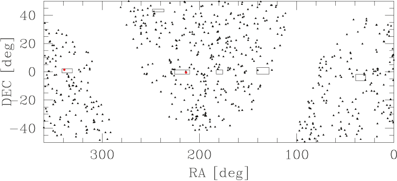
We now correlate our mass map peaks with published X-ray clusters to compare the selection functions of lensing and X-ray cluster searches. Piffaretti et al. (2011) sorted out catalogs of X-ray clusters to generate a useful meta-catalog, called MCXC. Among them, we are interested in the catalogs based on the ROSAT All Sky Surveys (RASS) composed of the northern NORAS and southern REFLEX (Voges et al., 1999). Figure 6 shows the sky distribution of the NORAS/REFLEX clusters compiled in the MCXC catalog. The Figure indicates that our survey fields are buried well within the area where the X-ray clusters were searched. We find that two peaks are matched with the X-ray clusters under the tolerance of $5^{\prime}$ (see Table 2). Here we adopt the slightly increased tolerance radius of $5^{\prime}$ following the argument by Shan et al. (2012) where they argue the existence of additional noise in the X-ray centers. The Table also shows that there are two X-ray clusters which are within our survey field but have no counterpart in the peak list. The redshifts are 0.0175 and 0.1259, respectively, and the latter has a counter part in the CAMIRA catalog although the former does not because of its low redshift value (the CAMIRA cluster catalog is constructed only at $z>0.1$). The locations of these four X-ray clusters are shown by large open triangles in Figures 1, 2, and 3.

Table 2: Comparison of the peaks with the MCXC X-ray cluster catalog

rank	$z^{(1)}$	$M_{\rm 500,WL}$	$M_{\rm 500(MCXC)}$	$L_{\rm 500,(MCXC)}$	Abell	MCXC
		[$\times 10^{14}M_{\odot}$]	[$\times 10^{14}M_{\odot}$]	[$\times 10^{44}{\rm erg\,s^{-1}}$]
6	0.0594	2.5$\pm$0.6	1.8	0.88	2457	J2235.6+0128
26	0.1403	2.8$\pm$0.9	2.8	1.9	1882	J1415.2-0030
-	0.0175	$<0.5$ (2$\sigma$)	0.13	0.011	-	J0920.0+0102
-	0.1259	$<0.6$ (2$\sigma$)	1.2	0.47	-	J1415.8+0015

Two MCXC clusters are matched with the peaks under the tolerance of $5^{\prime}$. The last two X-ray clusters do not have the counterparts in our peak list. The redshifts $z^{(1)}$ are taken from the MCXC catalog. $L_{\rm 500,(MCXC)}$ is measured in the 0.1 – 2.4 keV band.

Figure 6: Sky distribution of NORAS/REFLEX clusters compiled in the MCXC catalog (solid triangles) and the survey area of HSC-Wide S16A analyzed in this paper (rectangles). The MCXC clusters that are matched with the peaks are shown in red filled circles. There are four clusters in our survey regions, and among them, two are matched with the peaks.

One of our survey field is designed to overlap with the wide field survey by the XMM-Newton satellite called XXL (Pierre et al., 2016). We compare the peak list with X-ray clusters published in Pierre et al. (2016). The location of the XXL brightest 100 clusters are presented as small open triangles in Figure 1. In the overlap region, we find 39 XXL clusters among which three weak lensing peaks are matched under the tolerance of $5^{\prime}$, as is summarized in Table 3. Turning the problem around, two peaks do not have any counterparts in the cluster catalog although they are well inside the XXL survey footprint.

Table 3: Comparison of the peaks with the XXL brightest 100 X-ray cluster catalog

rank	$z$	$M_{\rm 500,WL}$	XLSSC	$M_{\rm 500,MT(XXL)}$	$L_{\rm 500(XXL)}$	$M_{\rm 500,WL(XXL)}$
		[$\times 10^{14}M_{\odot}$]		[$\times 10^{14}M_{\odot}$]	[$\times 10^{44}{\rm erg\,s^{-1}}$]	[$\times 10^{14}M_{\odot}$]
2	0.186	3.9 $\pm$ 0.7	091	5.1 $\pm$ 2.2	1.31 $\pm$ 0.02	6.2${}^{+2.1}_{-1.8}$
36	0.155	1.7 $\pm$ 0.5	041	1.0 $\pm$ 0.4	0.12 $\pm$ 0.007	0.7${}^{+0.6}_{-0.5}$
58	0.287	2.6 $\pm$ 1.1	111	4.0 $\pm$ 1.8	0.67 $\pm$ 0.03	6.3$\pm$1.8
28	0.276	2.4 $\pm$ 0.7	-	-	-	-
43	0.272	2.5 $\pm$ 0.9	-	-	-	-

Three XXL clusters are matched with the peaks under the tolerance of $3^{\prime}$. The last two peaks do not have the counterparts in the brightest 100 XXL clusters. The redshifts $z$ are taken from the CAMIRA catalog. $M_{\rm 500,XXL-T}$ are taken from Pacaud et al. (2016), and $M_{\rm 500,XXL-WL}$ from Lieu et al. (2016). $L_{\rm 500(XXL)}$ is measured in the 0.5 – 2 keV band.

4.3 Mass estimate of the clusters

For each peak, we estimate the cluster mass from the observed tangential shear radial profile which is azimuthually averaged in the annulus. We assume that the density of the dark matter halos follows the NFW profile

$$\rho(r)=\frac{\rho_{s}}{\left(r/r_{s}\right)\left(1+r/r_{s}\right)^{2}},$$ (11)

where $\rho_{s}$ is the characteristic density and $r_{s}$ is the scale radius. The two-dimensional surface mass density is computed as

$$\Sigma(R)=2\int_{0}^{\infty}\rho(R,y)dy,$$ (12)

where $R$ is the projected radial distance. The differential surface mass density is then given by,

$$\Delta\Sigma(R)\equiv\bar{\Sigma}(<R)-\Sigma(R),$$ (13)

and

$$\bar{\Sigma}(<R)=\frac{2}{R^{2}}\int_{0}^{\infty}\Sigma(R^{\prime})R^{\prime}dR^{\prime}=r_{s}\rho_{s}g(R,r_{s}),$$ (14)

where $g(R,r_{s})$ is given by equation (8) in Ford & VanderPlas (2016).

In this paper, we define the cluster radius $r_{\Delta}$ within which the mass density is a factor of $\Delta$ larger than the critical mass density, $\rho_{c}$. The mass inside the $r_{\Delta}$ is naturally calculated as

$$M_{\Delta}=\frac{4}{3}\pi r_{\Delta}^{3}\rho_{c}\Delta.$$ (15)

Here we introduce the concentration parameter $c_{\Delta}$ as

$$c_{\Delta}=\frac{r_{\Delta}}{r_{s}}$$ (16)

In the mean time, Navarro et al. (1997) showed that $\rho_{s}$ is given by

$$\rho_{s}=\rho_{c}\frac{\Delta c^{3}_{\Delta}}{3\left[\ln{(1+c_{\Delta})}-c_{\Delta}/(1+c_{\Delta})\right]},$$ (17)

where we adopt $\Delta=500$ in this paper.

Observationally, the differential surface mass density, $\Delta\Sigma(R)$, is constrained by the tangential shear $\gamma_{T}(R)$. In the case of spherically symmetric dark matter halo which we assume throughout this paper,

$$\Delta\Sigma(R)=\Sigma_{\rm cr}\gamma_{T}(R),$$ (18)

where

$$\Sigma_{\rm cr}=\frac{c^{2}}{4\pi GD_{l}}\left<\frac{D_{ls}}{D_{s}}\right>^{-1},$$ (19)

with $D_{l}$, $D_{ls}$, $D_{s}$ being the angular diameter distances to the lens, between the lens and source galaxies and to the source, respectively. The distance factor, $D_{ls}/D_{s}$ is averaged over the background source galaxies whose photometric redshift is 5% larger than the redshift of the lens.

By fitting the radial profile of the tangential profile, we can constrain ($\rho_{s}$, $r_{s}$) using equations (13), (14), and (18), and then ($M_{\Delta}$, $c_{\Delta}$) is obtained using equations (15) to (17). We assume a flat cosmology where $\rho_{c}(z)$ is given by

$$\rho_{c}(z)=\rho_{c}(z=0)\left[\Omega_{M0}(1+z)^{3}+\Omega_{\Lambda 0}\right].$$ (20)

Fitting is made in the physical scale between 0.2 to $7h^{-1}$Mpc for all cases.

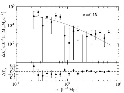
As an example, Figure 7 shows the observed radial profile of differential surface mass density for rank 4 peak. The error of each point is estimated from the orthogonal shear component. The best-fit NFW profile is shown by the solid line, which have the mass and the concentration parameter values of ($M_{500}$, $c_{500}$) = ($(2.97\pm 0.69)\times 10^{14}h^{-1}M_{\odot}$, $2.1\pm 1.0$). We present the ($M_{500}$, $c_{500}$) of all isolated peaks (that matched with one CAMIRA cluster) in Table 4. The mass of multiply matched peaks are not shown to avoid confusion. We note that the constraint on the concentration parameter is poor for these individual peak analysis because the constraint in the inner region is limited.

The measured mass depends largely on the outskirts of the dark matter halo and we do not include the central part of the shears for fitting in order to avoid the influence from dilution effect (See. 5.4), the error caused by the uncertainties of the dark matter halo center is negligible.

Figure 7: Radial profile of the differential surface mass density of rank 4 peak. The best-fit NFW model to the data is shown by the solid line. Bottom panel shows the profile generated by B-mode components.

5 Discussions

5.1 Number of the observed peaks

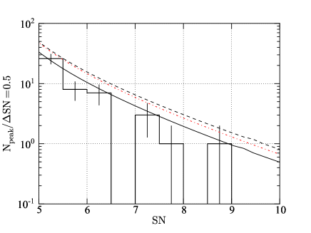
We compare the observed numbers of peaks with the analytic model calculation, which is presented in Appendix 1. The analytic model is verified by the peak numbers derived from 100 mock galaxy catalogs from all-sky $N$-body simulations with ray-tracing calculations (Oguri et al., 2017b; Takahashi et al., 2017). The observed peak count is shown in Figure 8 as a histogram whereas the peak counts expected from the analytical model assuming the WMAP nine year cosmological parameter results (Hinshaw et al., 2013) is shown as a solid line (hereafter WMAP9). We see a good agreement between the observation and the model. Dashed line in the figure shows the expected peak count assuming the Planck 2015 cosmological parameter results (Planck Collaboration et al., 2016a) whose $\sigma_{8}$ is higher than that of WMAP9 (hereafter Planck15). The result suggests that our observation favors the low $\sigma_{8}$ WMAP9 cosmology. We estimate the effect of the dilution by cluster member galaxies (see Appendix 2 for details), and find that it is not sufficiently large to change our conclusion. However, as discussed in Appendix 2, our calculation may underestimate the dilution effect. More careful assessment of the dilution effect should be made before drawing any firm conclusion.

Figure 8: The histogram with error bars shows the observed peak count. The solid line and the dashed line present the expected peak counts from analytic models based on WMAP9 and Planck15 cosmology, respectively. The details of the analytic model is presented in Appendix 1. Dash-dotted line presents the peak count with Planck15 cosmology where dilution by member galaxies are considered (see Appendixes 2 to see how the dilution is modeled). The lines show the numbers of mass map peaks integrated over the same bin size of $\Delta\nu=0.5$ as that used for the histogram, i.e., the line value at each $\nu$ indicates the predicted total number of mass map peaks between $\nu-0.5\Delta\nu$ and $\nu+0.5\Delta\nu$.

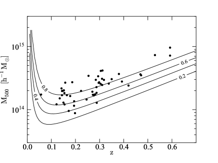
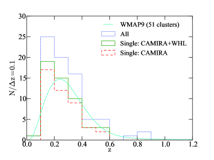
In addition to the comparison of the number counts, the analytic model allows us to estimate the the selection function of the shear selected cluster sample. Figure 9 compares the selection function in the the $M_{\rm 500}$-$z$ plane derived from the analytic model is compared with estimates of $M_{\rm 500}$ for individual peaks from fitting of tangential shear profiles presented in Section 4.3. We find that masses and redshifts of individual peaks are indeed located in the relatively high completeness region of the $M_{\rm 500}$-$z$ plane. The expected number counts of shear selected clusters are obtained by combining the completeness with the mass function of dark halos. Figure 10 compares the redshift distribution of our shear selected cluster sample with the theoretical expectation, which again shows a good agreement. The well-defined selection function is one of the biggest advantages of a shear selected cluster sample.

Figure 9: Completeness of shear selected clusters ($\nu>4.7$) estimated from the analytic model, assuming the WMAP9 cosmology (Solid line contour) in the $M_{\rm 500}$-$z$ plane (Eqn.(30)). Filled circles show the masses and redshifts of individual peaks, where the masses are estimated from tangential shear fitting. Here we show only isolated peaks for which only one CAMIRA clusters are matched.

Figure 10: The redshift distribution of shear selected clusters. Solid and dashed histograms show the observed redshift distributions for peaks that match CAMIRA only and CAMIRA+WHL15 catalogs, respectively. The dotted histogram shows the redshift distribution of peaks including those that have multiple counterparts in the CAMIRA catalog. The solid line shows the expected redshift distribution derived from the analytic model, with its amplitude normalized to the total number for the single CAMIRA case.

5.2 Weak lensing masses of X-ray clusters

We find that two peaks have counterparts in the MCXC catalog (Section 4.2), both of which are Abell clusters. Table 2 presents the mass estimates for these clusters, both from the tangential shear lensing signals and from the X-ray luminosity from Piffaretti et al. (2011). Although the error associated with X-ray mass estimate is not given in the literature, at least a level of 20% error is expected considering the large intrinsic scatter in the $L_{X}$-$M_{X}$ relation. Therefore, we find that both the lensing and the X-ray mass estimates are consistent for these two clusters.

There are two other MCXC clusters inside our survey area, for which no counterpart is found in the shear selected cluster catalog. One is MCXC J0920.0+0102 at the redshift of 0.0175 whose mass estimated from X-ray luminosity is $0.13\times 10^{14}M_{\odot}$. Because the redshift of the cluster is too low, the lensing efficiency is small for this cluster and as a result the probability to detect the clusters of that mass is less than 10% according to Figure 9. The other one is MCXC J1415.8+0015 at $z=0.1259$ with the mass of $1.2\times 10^{14}M_{\odot}$ which is inconsistent with our 2$\sigma$ upper limit of $0.6\times 10^{14}M_{\odot}$. From Figure 9, we estimate that the probability to detect a cluster with the mass and redshift of MCXC J1415.8+0015 is 80%. Therefore, the discrepancy between the two mass estimates is not negligible for this cluster. In summary, the weak lensing mass estimates of three out of four clusters are consistent with those from X-ray, whereas one cluster shows mild inconsistency in the mass estimates.

Figure 11: Distributions of shear selected clusters (large black circles) and the NORAS/REFLEX X-ray clusters compiled in the MCXC catalog (small blue circles) on the $M_{\rm 500}$-$z$ plane . Two MCXC clusters that are matched with the shear selected cluster sample are shown by red squares. The solid line shows the typical lower mass limit of MCXC clusters estimated from the flux limit of $1.8\times 10^{-12}{\rm erg\,s^{-1}cm^{-2}}$ combined with the $L$-$M$ relation given by the equation (10) in Böhringer et al. (2014).

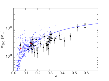
Figure 11 presents the comparison of the shear selected clusters with the MCXC clusters in the the $M_{\rm 500}$-$z$ plane. Among the shear selected clusters, those that are matched with single CAMIRA clusters are shown here to guarantee the accuracy of the weak lensing mass estimates. This comparison indicates that weak lensing shear tends to probe less massive clusters toward higher redshifts, although there is an overlapping region in which clusters from both the cluster samples are distributed. We are particularly interested in shear selected clusters above the typical mass limit of MCXC estimated from the flux limit of $1.8\times 10^{-12}{\rm erg\,s^{-1}cm^{-2}}$ combined with the $L$-$M$ relation given by the equation (10) in Böhringer et al. (2014) (solid line in Figure 11) and the redshift below 0.2 where mass estimates are expected be more robust. There are five peaks in our catalog that satisfy this criterion, which are summarized in Table 4. We check the XMM, Chandra and Suzaku X-ray archives to identify X-ray counterparts for these five peaks, and find that peak rank 31 has its counterpart in the Chandra archive. Because the X-ray source falls in the gap of the Chandra CCDs, only partial image is obtained. The X-ray emission is extended, and from the partial image we derive the lower limit of the X-ray source to be $2.2\times 10^{43}{\rm erg\,s^{-1}}$.

For the other four peaks (rank 3, 24, 38, 46), neither Suzaku, XMM-Newton, nor Chandra archive data are currently available. We thus estimate the X-ray luminosity of each cluster from the RASS spectrum integrated from a circular region centered on the peak. The extraction radius is $1^{\prime}$ ($\sim 1$ Mpc) for rank 3, 38, 46, whereas it is $9^{\prime}$ for rank 46 because of the lack of data within $6^{\prime}$. Assuming that the observed RASS spectrum is represented by a sum of ICM thermal emission, the Galactic soft X-ray emission (0.1 keV Local Hot Bubble and 0.3 keV Milky Way Halo components), and the comic X-ray background (Kushino et al., 2002), we perform the spectral fitting and derive the $3\sigma$ upper limit on the 0.1–2.4 keV X-ray luminosity (Table 4). Here the APEC thermal plasma model (Smith et al., 2001) is assumed for the ICM component and the temperature and the metal abundance are fixed at 5 keV and 0.3 solar, respectively. From a comparison with the mass-luminosity relations given in Figure 3 of Giles et al. (2015), it appears that shear-selected clusters tend to be underluminous in X-ray. Due to large uncertainties associated with the present analysis, however, further deep observations using Chandra or XMM-Newton would be essential to constrain X-ray temperature and other properties. In fact, inside the search radius of $3^{\prime}$, two peaks, rank 24 and 38, are found to have faint X-ray sources on the second ROSAT all-sky survey catalog (Boller et al., 2016); 2RXSJ162010.5+422811, 2RXSJ120955.7-003234, respectively.

Table 4: Massive shear selected clusters that has no counterpart in the MCXC X-ray cluster catalog

rank	$z$	$M_{\rm 500,WL}$	$L_{500,X}$
		[$\times 10^{14}$M⊙]	[$\times 10^{43}$erg/s]
3	0.1540	2.6$\pm$0.6	$<$ 6
24	0.1473	3.1$\pm$1.2	$>$ 2.2
31	0.1420	2.8$\pm$0.8	$<$ 6
38	0.1780	2.3$\pm$0.8	$<$ 8
46	0.1575	3.9$\pm$1.2	$<$ 8

We find the counterpart of the peak 32 on Chandra archive. All the other upper limit come from RASS.

We then compare the masses of the four clusters that have matched with the published X-ray clusters in the XXL survey. The mass estimate XXL cluster is based primarily on the X-ray temperature inside the fixed 300 kpc aperture which was calibrated by the weak lensing data taken by CFHT Legacy Survey (Lieu et al., 2016). The results shown in Table 3 indicate that our weak lensing mass estimates are consistent with the XXL mass estimates for the four clusters. This is somehow inconsistent with the suggestion by Giles et al. (2015) that weak lensing selected clusters tend to be embedded in the filaments viewed near the line-of-sight and the mass tends to be overestimated by the filaments. Hamana et al. (2012) also argued, based on ray-tracing simulations and an analytic halo model, that shear selected clusters exhibit the orientation bias such that their major axes are preferentially aligned with line-of-sight direction, which also induces the mismatch between lensing and X-ray masses. We see no evidence of such a bias in our weak lensing selected samples shown above, presumably due to the small sample size.

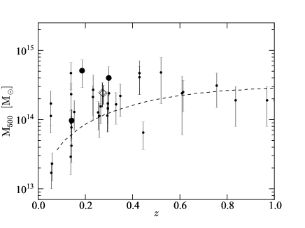
In the cross-match of the peaks with the published XXL clusters, there are two peaks that do not have counterparts in the XXL cluster list. We show these samples in the $M_{\rm 500}$-$z$ plane in Figure 12, together with other XXL clusters inside our HSC S16A survey area. Both peaks are located above the 50% completeness limit of the XXL cluster sample. Therefore, given their lensing masses these clusters should have been detected by XXL, assuming that these clusters follow the standard mass-luminosity scaling relation. We note, however, that the XXL cluster catalog was constructed by using both X-ray core size and flux, and therefore such non-detected clusters might be more extended rather than under-luminous. Further studies over wide field is vitally important to understand X-ray gas properties and also to study some other systematic bias in different techniques to search clusters. The eROSITA will provide a good opportunity to conduct this type of work.

Figure 12: The distribution of XXL clusters in the $M_{\rm 500}$-$z$ plane. Small filled circles indicate XXL clusters inside our HSC S16A survey area, whereas large filled circles are XXL clusters that are matched with the lensing peaks. Open diamond show the redshifts and lensing masses of shear selected clusters that do not have counterparts in the XXL cluster catalog. Dashed line shows the 50 % completeness limit of the XXL cluster sample.

Figure 13: The stacked $0.5-2.0$ keV RASS images of shear selected clusters (left panel) and MCXC selected clusters (right panel) selected to have X-ray luminosity greater than that expected for our mass threshold. The images have been smoothed by a 9 pixel gaussian kernel. The scale in the left (right) panel correspond to the mean counts per second expected from a cluster that went into the stack at the median redshift of $z=0.27$ ($z=0.14$).

5.3 Stacked X-ray emission

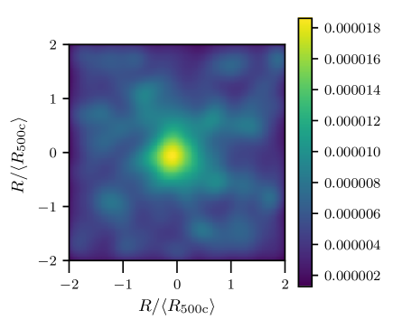
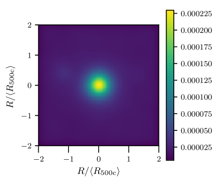
As we were able to identify only a limited number of X-ray counterparts for the shear-selected peaks, we stack the X-ray emission from ROSAT around the shear selected peaks with a procedure somewhat similar to Anderson et al. (2015). As the shear peaks have limited centering accuracy, we used the position and redshift of the optical cluster counterparts that correspond to our shear-selected peaks. We first extract a RASS image in the energy band (0.5-2.0) keV around the optical counterparts extending out to the mean $2R_{\rm 500c}$, as well as the corresponding RASS exposure map. Dividing the RASS image by the exposure map, yields an image with the counts per second for each cluster. We then perform a weighted addition of these RASS images together to produce a stacked image. The weight we use $D_{\rm L}^{2}(z)/D_{\rm L}^{2}(z_{\rm med})$, standardizes the flux to its expectation at the median redshift of our shear selected clusters ($z_{\rm med}=0.27$). Known point sources are excluded in the stacking procedure. Such a stacked image is shown in Figure 13 and shows that we can clearly detect emission from our shear-selected clusters once they are stacked. We have checked that our stacked image is similar even if we first stack the raw count images and divide by the total exposure at the end.

We then compute the count rate of X-ray photons within $R_{\rm 500c}$ for the average mass and subtract the expected count rate due to the background estimated within an annulus of $[1,2]R_{\rm 500c}$. We obtain a net count rate $(3.2\pm 0.6)\times 10^{-2}$ cnt/s, where the errors on the count rates were estimated using the jackknife technique. These count rates are then converted to a X-ray luminosity assuming a metallicity which is 0.2 solar, the average column density $\langle N_{H}\rangle=3\times 10^{20}{\rm cm}^{-2}$. The X-ray luminosity we obtain for our shear selected clusters is $L_{\rm x}=(1.5\pm 0.3)\times 10^{44}{\rm ergs^{-1}}$ in the $0.1-2.4$keV.

To compare with X-ray selected clusters, we similarly stacked the RASS images around clusters in MCXC catalog Piffaretti et al. (2011) with an X-ray luminosity greater than that expected given the mass-detection threshold for our shear-selected clusters (see Figure 9). We also applied the following selection criteria $0.01<N_{H}/10^{22}{\rm cm^{-2}}<0.06$ and $0.01<z<0.6$ which corresponds to the same range as those for shear-selected clusters. The average X-ray luminosity of these clusters based on the MCXC catalog is $L_{\rm x}=2.9\times 10^{44}{\rm ergs^{-1}}$ in the $0.1-2.4$keV band. Our procedure for computing $L_{\rm x}$ based on the stacked RASS image (see right panel of Figure 13) yields $(29\pm 2)\times 10^{-2}$ cnt/s at a median redshift of $z=0.14$. This corresponds to $L_{\rm x}=(3.1\pm 0.2)\times 10^{44}{\rm ergs^{-1}}$ in agreement with the average value based on the MCXC catalog. This shows that the X-ray luminosity of our shear-selected clusters is about half of that expected from X-ray selected clusters at $\sim 5\sigma$ level. Since the shear-selected clusters are unbiased to selection effects in X-ray surveys concerning X-ray luminosity and dynamical states, this demonstrates its potential power to discover X-ray underluminous clusters. Once selection effects due to orientation biases are accounted, the shear selected clusters could potentially provide hints to resolving the discrepancy in the number of clusters discovered through the SZE (Planck Collaboration et al., 2016b) or X-ray (Pacaud et al., 2016) method and the predictions for these abundances based on cosmological parameters inferred from the cosmic microwave background observations (Planck Collaboration et al., 2016a).

5.4 Average radial density profile of clusters from stacked lensing

The lensing signal depends both on the total mass of the cluster and its radial density profile. More concentrated clusters are more likely to be detected by lensing. In order to see how our weak lensing clusters sample differs from clusters studied so far, we check the average radial density profile of our sample. As is presented in Figure 7, lensing signals from individual clusters are not sufficient to constrain the radial profile accurately. Instead, we carry out a stacked lensing analysis. We compute the differential surface mass density (equation 18) for each cluster. We select source galaxies behind the cluster based on the photometric redshift. We then stack them to obtain the average differential surface mass density

$$\Delta\Sigma(R)=\left<\Sigma_{\rm cr,i}\gamma_{T,i}(R=D_{l,i}\theta)\right>$$ (21)

where we calculate averaged $\Sigma_{\rm cr}$ for each $i$-th cluster and the angular separation from the center, $\theta$, is scaled to physical length when stacking.

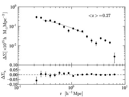
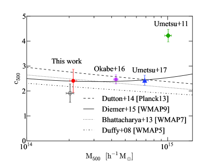
Figure 14 shows the stacked differential surface density profile around 50 weak-lensing peaks that are matched with single isolated CAMIRA clusters. The average redshift of the sample is $0.27$. The data is fitted to an NFW profile on the physical scale between $0.3$ to $1.7h^{-1}$Mpc to obtain the mass, $M_{500}$ and the concentration parameter, $c_{500}$ as $(2.03\pm 0.13)\times 10^{14}h^{-1}M_{\odot}$ and $1.91\pm 0.37$, respectively. Here we adopted $1.7h^{-1}$Mpc for the outer radius limit to avoid possible contamination from 2-halo term. This result is shown in Figure 15 as a open circle.

In projection, the 2-halo term is nearly constant out to about 3 virial radii, so that the 2-halo contribution to the differential surface mass density ($\Delta\Sigma$) is negligible at small cluster-centric distances, and it becomes dominant only at large distances, R $\sim$ 5 virial radii (Oguri & Hamana, 2011). These expected behaviors are consistent with recent cluster weak-lensing observations (e.g. Okabe & Smith (2016)), and the NFW density profile provides an excellent description of the projected matter distribution around clusters out to about 2 virial radii (Umetsu et al., 2016). Therefore, the 2-halo term with in the physical scale of $1.7h^{-1}$ Mpc is negligible.

If cluster member galaxies are mis-identified as background galaxies, the observed lensing signal can be systematically underestimated progressively toward the cluster center (Medezinski et al., 2010), in proportion to the fraction of unlensed galaxies whose orientations are randomly distributed. This dilution effect is a major source of cluster weak-lensing measurements, and is not accounted for in our analysis described above. To establish optimal source selection schemes for unbiased cluster weak-lensing measurements, Medezinski et al. (2017) examined the degree of cluster contamination by analyzing a large sample of $\sim 900$ CAMIRA clusters with richness greater than 20 identified in $\sim 160$ deg² of HSC-SSP data. According to the findings of Medezinski et al. (2017) (see Figure 10 of Medezinski et al. (2017)), the level of dilution reaches up to $15\%$ at a cluster-centric radius of $r=0.3h^{-1}$ Mpc and becomes less than $10\%$ at $r\gtrsim 0.5h^{-1}$ Mpc. We account for this dilution effect by applying corrections obtained by Medezinski et al. (2017) at each cluster radius $r$. The filled circle in Figure 15 shows the best-fit $c$–$M$ relation ($M_{500}=(2.13\pm 0.13)\times 10^{14}h^{-1}M_{\odot}$, $c_{500}=2.41\pm 0.46$) derived from our stacked lensing analysis after correcting for the dilution effect. Compared with the original estimates (open circle), the dilution correction increases $M$ and $c$ by 5 % and 26 %, respectively. Note that $M$ and $c$ in Table 4 are the values before the dilution correction.

Mis-centering of dark matter concentration can also lower estimates of the concentration parameter. Here, we adopted the peak position as the center, whose uncertainty is expected to be an order of the smoothing scale that we adopted, i.e., $\sim 1^{\prime}$. This angular scale is smaller than the innermost radius of radial profile fitting, $0.3h^{-1}$ Mpc, for the clusters below the redshift of 0.5 where most of our samples are located. Thus the mis-centering does not affect the estimate of the concentration parameter significantly.

It is interesting to adopt the CAMIRA’s BCG positions as the center of halo and to try the same stacking analysis. The best fit parameter that obtained through this trial is ($M_{500}$, $c_{500}$) = ($1.78\pm 0.12)\times 10^{14}h^{-1}M_{\odot}$, $1.13\pm 0.23$). Compared with the original estimates, the mass does not change significantly whereas $c$ drops largely. This suggests that the adoption of the BCG position in fact increase the degree of mis-centering of the dark matter halos, which is consistent with the expectation as discussed in Sec. 4.1.

Several groups have reported observational results from NFW fits to the lensing profiles of X-ray luminous clusters (Umetsu et al., 2009; Okabe & Smith, 2016; Umetsu & Diemer, 2017). They obtained $c_{\mathrm{vir}}\sim 6$ for $M_{\mathrm{vir}}\sim 10^{15}h^{-1}M_{\odot}$ clusters, which corresponds to $c_{\mathrm{500}}\sim 3$ and is consistent with our results. Mandelbaum et al. (2006) estimated the mass-concentration relation using galaxy-galaxy lensing based on the SDSS data and showed that $c_{\rm vir}=5\pm 1$ ($c_{500}\sim 2.5$) in our mass range. Therefore, our estimate is also consistent with their result.

On the other hand, Umetsu et al. (2011) obtained $c_{\mathrm{vir}}=7.68^{+0.42}_{-0.40}$ from spherical NFW fits for a sample of four strong-lensing-selected superlens clusters with $M_{\mathrm{vir}}\simeq 1.5\times 10^{15}h^{-1}M_{\odot}$, corresponding to $c_{\mathrm{500}}=4.22\pm 0.25$ at $M_{\mathrm{500}}=(10.08\pm 0.58)\times 10^{14}h^{-1}M_{\odot}$. The superlens sample is characterized by large Einstein radii $>30$ arcsec (for a fiducial source redshift of $z=2$). Their concentration is apparently higher than our $c$ measurement of the shear selected clusters. Oguri et al. (2012) found similarly high concentration parameter estimates for their strong-lensing clusters selected from SDSS data. This discrepancy can be solely explained by the selection and projection bias of strong-lensing-selected clusters as discussed in Oguri et al. (2012) and Umetsu & Diemer (2017).

Since the lensing-derived concentration parameter is sensitive to the selection and projection effects, if we obtain a halo concentration that is consistent with the theoretical mass-concentration relation, it may imply that shear selected cluster populations of clusters are statistically different from those selected by the strong-lensing properties and they are not biased toward very high concentrations. Unlike strong-lensing-selected cluster samples, our weak lensing clusters are selected primarily because they are massive. While Hamana et al. (2012) predicted the moderate orientation bias for shear selected clusters, the bias is predicted to be much weaker than that for strong-lensing-selected clusters. Therefore we may need a much larger sample of shear selected clusters to find any possible evidence of the selection bias for shear selected clusters. A caveat is that Hamana et al. (2012) predicted larger orientation bias for higher $\nu$ peaks, which should also be tested with observations.

In Figure 15, several numerical predictions are shown, including Duffy et al. (2008), Dutton & Macciò (2014), Bhattacharya et al. (2013), and Diemer & Kravtsov (2015), where different models are calibrated for different $\Lambda$CDM cosmologies. For the Diemer & Kravtsov (2015) model, which is applicable for any cosmology, we assume the WMAP9 cosmology. Combined with the result with Umetsu & Diemer (2017) and taking the dilution correction into account, we slightly disfavor the prediction by Duffy et al. (2008) which assumes WMAP5 in their calculation.

The cluster mass-concentration relation is sensitive to cosmological parameters. In particular, its normalization is highly sensitive to the combination of $\Omega_{\mathrm{m}}$ and $\sigma_{8}$, As demonstrated in Dutton & Macciò (2014), more recent cosmological models (since WMAP3) take higher values of ($\Omega_{\mathrm{m}},\sigma_{8}$), thus predicting a higher normalization in the mass-concentration relation. This may explain the inconsistency against Duffy et al. (2008) adopting WMAP5 whose normalization is lower than the later WMAP and Planck.

Among the concentration models considered here, all except Diemer & Kravtsov (2015) show a monotonic decrease of $c$ as $M$ increases. Diemer & Kravtsov (2015), however, predicts an upturn at high masses due to dynamically un-relaxed, forming halos (Ludlow et al., 2010). With the full survey data in hand where we expect more than a six times larger sample, we will be able to distinguish these concentration models and to observationally establish the mass-concentration relation over a wide range of the cluster mass and the redshift.

Figure 14: Stacked differential surface density profile from about 50 shear selected clusters. The solid line shows the best-fit model assuming the NFW density profile. Fitting is made in the physical scale between $0.3$ to $1.7h^{-1}$Mpc. Photometric redshifts of individual galaxies are used to select background galaxies. The best-fit values are ($M_{500}$, $c_{500}$) = (($2.03\pm 0.13)\times 10^{14}h^{-1}M_{\odot}$, $1.91\pm 0.37$). Bottom panel shows the profile generated by B-mode components.

Figure 15: Constraints on the mass-concentration relation. The result of the fitting of the NFW profile to the stacked differential surface density for about 50 shear selected clusters (see Figure 14) is shown by the open circle. After the dilution correction (see text), the constraint is shifted to the point shown by the filled circle. The average redshift of the shear selected clusters is 0.27. The filled triangle shows the results for 16 X-ray-selected clusters at an average redshift of 0.34 obtained from a strong and weak lensing analysis of Umetsu & Diemer (2017). The filled diamond shows the results for a sample of 4 strong-lensing-selected superlens clusters at an average redshift of 0.32 from a strong and weak lensing analysis of Umetsu et al. (2011). The filled square is from Okabe & Smith (2016) estimated from 50 X-ray luminous (LoCuSS) clusters at redshift between 0.15 and 0.3

6 Conclusion

We have constructed a shear selected cluster catalog containing 65 mass map peaks with $\nu>4.7$ from the HSC-SSP Wide S16A dataset covering $\sim 160$ deg². The cluster catalog is large in size yet has small contaminations from false positives. We have found that all the mass map peaks with $\nu>5.1$ have physical counterparts, and only 2 out of the 65 clusters are probably false positives. The peak counts are found to be consistent with the predictions from WMAP9 cosmology but the tension appears to exist if we adopt the Planck15 cosmology. The comparison with the published X-ray catalogs have shown that cluster masses estimated from lensing are consistent with X-ray mass estimates, although the matched sample is small. On the other hand, there exist a few X-ray undetected shear selected cluster candidates which should have been detected by the existing X-ray surveys if the clusters follow the standard mass-luminosity relation. We stacked RASS X-ray images around the shear-selected clusters and compare with X-ray selected clusters given the same selection function of the mass. We found that the average X-ray luminosity for the shear-selected clusters are about half of that of the X-ray selected clusters at the $\sim 5\sigma$ level. It indicates the existence of the population of X-ray underluminous clusters and that the shear-selection can discover such a population. Future studies to constrain the abundance of such clusters are necessary. Stacked lensing analysis suggests that the average radial mass profile of the shear selected clusters is not too concentrated, which implies that shear selected clusters do not exhibit strong selection bias on the orientation or the internal structure, and that the clusters are selected basically because they are massive.

This paper presents the initial results on shear selected clusters from the HSC-SSP survey. At the completion of the HSC-SSP survey, the shear selected cluster sample would potentially be at least six times larger, which is sufficiently large to conduct various statistical studies with high accuracy.

This work was supported in part by World Premier International Research Center Initiative (WPI Initiative), MEXT, Japan, and JSPS KAKENHI Grant Number 15H05892, 26800093. MO and SM acknowledges financial support from JST CREST Grant Number JPMJCR1414. SM is also supported by the Japan Society for Promotion of Science grants JP15K17600 and JP16H01089.

The Hyper Suprime-Cam (HSC) collaboration includes the astronomical communities of Japan and Taiwan, and Princeton University. The HSC instrumentation and software were developed by the National Astronomical Observatory of Japan (NAOJ), the Kavli Institute for the Physics and Mathematics of the Universe (Kavli IPMU), the University of Tokyo, the High Energy Accelerator Research Organization (KEK), the Academia Sinica Institute for Astronomy and Astrophysics in Taiwan (ASIAA), and Princeton University. Funding was contributed by the FIRST program from Japanese Cabinet Office, the Ministry of Education, Culture, Sports, Science and Technology (MEXT), the Japan Society for the Promotion of Science (JSPS), Japan Science and Technology Agency (JST), the Toray Science Foundation, NAOJ, Kavli IPMU, KEK, ASIAA, and Princeton University.

The Pan-STARRS1 Surveys (PS1) have been made possible through contributions of the Institute for Astronomy, the University of Hawaii, the Pan-STARRS Project Office, the Max-Planck Society and its participating institutes, the Max Planck Institute for Astronomy, Heidelberg and the Max Planck Institute for Extraterrestrial Physics, Garching, The Johns Hopkins University, Durham University, the University of Edinburgh, Queen’s University Belfast, the Harvard-Smithsonian Center for Astrophysics, the Las Cumbres Observatory Global Telescope Network Incorporated, the National Central University of Taiwan, the Space Telescope Science Institute, the National Aeronautics and Space Administration under Grant No. NNX08AR22G issued through the Planetary Science Division of the NASA Science Mission Directorate, the National Science Foundation under Grant No. AST-1238877, the University of Maryland, and Eotvos Lorand University (ELTE).

This paper makes use of software developed for the Large Synoptic Survey Telescope. We thank the LSST Project for making their code available as free software at http://dm.lsst.org.

Based in part on data collected at the Subaru Telescope and retrieved from the HSC data archive system, which is operated by the Subaru Telescope and Astronomy Data Center at National Astronomical Observatory of Japan.

HM is supported by the Jet Propulsion Laboratory, California Institute of Technology, under a contract with the National Aeronautics and Space Administration.

Appendix 1. Expected peak counts from weak lensing SN-map

Here we present a halo model prediction of the number counts of peaks, focusing on the high $\nu$ region where single clusters dominate the signals.

The signal to noise ratio $\nu$ defined in equation (10) considers only the pure statistical noise of the measurement, $\sigma_{\rm noise}$, which is proportional to $\sigma_{e}/\sqrt{N_{gal}}$, where $\sigma_{e}$ and $N_{gal}$ is the intrinsic galaxy ellipticity per component and the number of source galaxies, respectively. In the real cluster search with weak lensing mass peaks, the large-scale structure along the line-of-sight acts as a noise, which we describe as $\sigma_{\rm LSS}$. It can be computed from the cosmic shear power spectrum $C_{\ell}$ as

$$\sigma_{\rm LSS}^{2}=\int\frac{\ell d\ell}{2\pi}|\hat{U}(\ell)|^{2}C_{\ell},$$ (22)

where $\hat{U}(\ell)$ is the Fourier counterpart of the filter $U(\theta)$

$$\hat{U}(\ell)=2\pi\int\theta d\theta U(\theta)J_{0}(\ell\theta).$$ (23)

The cosmic shear power spectrum is related to the matter power spectrum $P_{m}(k;z)$ as

$$C_{\ell}=\int d\chi\frac{\left[W^{\kappa}(\chi)\right]^{2}}{\chi^{2}}P_{m}(k=\ell/\chi;z),$$ (24)

$$W^{\kappa}(\chi)=\frac{\bar{\rho}(z)}{(1+z)\Sigma_{\rm cr}(z)},$$ (25)

where the critical surface density $\Sigma_{\rm cr}$ is defined in equation (19). We fully take account of the redshift distribution of source galaxies by computing $\langle D_{ls}/D_{s}\rangle$ by averaging the distance ratios over the sum of the probability distribution functions of photometric redshifts of individual galaxies (Tanaka et al., 2017). For the matter power spectrum $P_{m}(k;z)$, we use the halofit model of Smith et al. (2003) and Takahashi et al. (2012).

For a single NFW halo with the mass $M$, the concentration parameter $c$, and redshift $z$, the peak SN $\nu_{\rm peak}$ is computed as

$$\nu_{\rm peak}=\frac{\kappa_{\rm peak}(M,c,z)}{\sigma_{\rm noise}},$$ (26)

$$\kappa_{\rm peak}(M,c,z)=2\pi\int d\theta\theta\kappa_{\rm NFW}(\theta;M,c,z)U(\theta),$$ (27)

where $\kappa_{\rm NFW}$ is the convergence profile for the NFW halo. Again, we include the redshift distribution of source galaxies in $\Sigma_{\rm cr}$ that is used to compute $\kappa_{\rm NFW}$. We then compute the number density of mass map peaks with $\nu_{1}<\nu<\nu_{2}$ as

$$\frac{dN}{d\Omega}(\nu_{1},\nu_{2}) = \int dz\frac{dV}{dzd\Omega}\int dM\frac{dn}{dM}\int dc\frac{dp}{dc}$$ (28)

$$\times S(M,z,c;\nu_{1},\nu_{2}),$$

where $dn/dM$ is a mass function of dark halos (Tinker et al., 2008), $dp/dc$ is the distribution of the concentration parameter which we assume log-normally distributed

$$\frac{dp}{dc}=\frac{1}{\sqrt{2\pi}\sigma_{\ln c}}\exp\left[-\frac{(\ln c-\ln\bar{c})^{2}}{2\sigma_{\ln c}^{2}}\right]\frac{1}{c}.$$ (29)

We use the model of the concentration parameter presented by Diemer & Kravtsov (2015), which takes account of the cosmology dependence of the concentration parameter as a function of halo mass and redshift. The selection function $S(M,z,c;\nu_{1},\nu_{2})$ is

$$S(M,z,c;\nu_{1},\nu_{2})=\frac{1}{2}\left[{\rm erfc}\left(x_{1}\right)-{\rm erfc}\left(x_{2}\right)\right],$$ (30)

$$x_{i}=\frac{1}{\sqrt{2(1+\sigma_{\rm LSS}^{2}/\sigma_{\rm noise}^{2})}}(\nu_{i}-\nu_{\rm peak}),$$ (31)

where we consider $\sigma_{\rm LSS}$ (equation 22) to incorporate the noise enhancement by large-scale structure. The selection function $S(M,z,c;\nu_{1},\nu_{2})$ take accounts of the scatter of peak heights due to the shot noise ($\sigma_{\rm noise}$) as well as random projections of halos along the line-of-sight ($\sigma_{\rm LSS}$). Given that this model includes the situation that $\nu$ of halos with relatively small masses are significantly boosted by $\sigma_{\rm LSS}$, peaks generated by projections of multiple small halos along the line-of-sight are taken into account in this model, at least to some extent.

In a simple case where the source galaxy density is uniform across the survey area, the shot noise $\sigma_{\rm noise}$ in equation (26) can be simply estimated as

$$\sigma_{\rm noise}=\sigma_{e}\sqrt{\frac{A}{n_{\rm g}}},$$ (32)

$$A=2\pi\int d\theta\theta Q^{2}(\theta),$$ (33)

where $\sigma_{e}$ is the rms error on the galaxy ellipticity per component. In practice, however, $\sigma_{\rm noise}$ is not uniform but has a spatial pattern due to the effects of the boundary, masking, and the inhomogeneous source number density. The spatial pattern of the noise $\sigma_{\rm sigma}$ can be estimated from the variance in mass maps using randomized galaxy shape catalogs, as done in Section 3.1. This allows us to derive the mass map area as a function of $\sigma_{\rm noise}$. Specifically, we denote $\Omega_{i}$ as the total area of mass maps that have the estimated shot noise $\sigma_{i}-\Delta\sigma/2<\sigma(\boldsymbol{\theta}_{0})<\sigma_{i}+\Delta\sigma/2$. In this case, the total number of mass map peaks with $\nu_{1}<\nu<\nu_{2}$ is given by

$$N_{\rm peak}(\nu_{1},\nu_{2})=\sum_{i}\left.\frac{dN}{d\Omega}(\nu_{1},\nu_{2})\right|_{\sigma_{\rm noise}=\sigma_{i}}\Omega_{i}.$$ (34)

Figure 16: Model predictions of the number counts of mass map peaks as a function of $\nu$. The solid line shows the analytic calculation (equation 34), whereas filled triangles with errors show the peak counts from mass maps with 100 mock shear catalogs (Oguri et al., 2017b). In both analytic and mock calculations, WMAP9 cosmology is assumed, and the multiplicative bias is set to $m=0$.

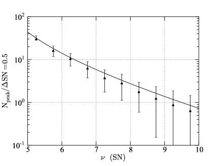
To check the accuracy of this analytic model prediction, we compare the number counts from equation (34) with results from mock shear catalogs. Oguri et al. (2017b) constructed mock shear catalogs for the first-year HSC shear catalog. The mock has the same spatial distribution as the real shear catalog from the observations, but the ellipticities of individual galaxies with mock ellipticity values. The mock ellipticity values are determined first by randomly rotating the orientations of individual galaxies and then adding cosmic shear taken from ray-tracing simulations (Takahashi et al., 2017). The comparison is given in Figure 16. In this comparison, we assume WMAP9 cosmology for both the analytic and mock calculations. The multiplicative bias is also set to $m=0$ for this comparison. We find a good agreement between the analytic model and mock result.

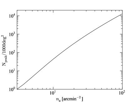
The analytic model allows us to explore the expected number density of mass map peaks as a function of various survey parameters. As a specific example, we predict the number density of mass map peaks with significant SN, $\nu>5$, as a function of the survey depth. Deep imaging increase both the source number density $n_{\rm g}$ and the mean source redshift $\bar{z}_{m}$. We include this correlation assuming a simple monotonic relation between these two as $n_{\rm g}=30\bar{z}_{m}^{3}$arcmin^-2, which roughly reproduces the observed trend. We also include the redshift distribution of the source galaxies assuming $n(z)\propto z^{2}\exp(-z/z_{0})$ with $z_{0}=\bar{z}_{m}/3$. The result shown in Figure 17 indicates that the peak number counts is indeed a very steep function of the survey depth. For example, the peak number density is enhanced by a factor of $\sim 20$ from $n_{\rm g}=10$ arcmin^-2 to $n_{\rm g}=30$ arcmin^-2. This prediction highlights the importance of deep imaging surveys as realized by the HSC-SSP survey for constructing a large sample of shear selected clusters.

Figure 17: The expected number of significant ($\nu>5$) mass map peak per 1000 deg² as a function of the source number density. In this calculation, we adopt a uniform $\sigma_{\rm noise}$, which is computed from the input source number density $n_{\rm g}$ and the intrinsic ellipticity of $\sigma_{e}=0.4$. In the calculation we also include the evolution of the mean source redshift as a function of $n_{\rm g}$ assuming the relation $n_{\rm g}=30\bar{z}_{m}^{3}$arcmin^-2.

Appendix 2. Dilution effect by cluster member galaxies

Member galaxies in clusters of galaxies do not contribute to lensing signals, and therefore dilute weak lensing signals. This is potentially one of the most significant sources of systematic effects in cluster weak lensing studies, and therefore has to be studied carefully. For instance, Kacprzak et al. (2016) studied the dilution effect and found relatively large corrections of $\nu$ of $\sim 10$% around $\nu\sim 4$ due to the dilution effect, for the case of Dark Energy Survey which is much shallower than the HSC-SSP. Here we employ a simple model of the number counts of cluster member galaxies to check the impact of the dilution effect on our results.

We use a model of the number of satellite galaxies as a function of the halo mass and redshift derived in Lin et al. (2004) and Lin et al. (2006) to estimate the dilution effect. We assume that the number density profile follow the NFW profile. Since these galaxies do not contribute to the lensing signals, the enhancement of the number density with respect to the average density represents the enhancement of the noise $\sigma_{\rm noise}$. We compute the enhancement of $\sigma_{\rm noise}$ as a function of the halo mass and redshift by convolving the number density profile of satellite galaxies with the filter function $Q(\theta)$, and include this in the halo model calculation described in Appendix 1. We find that the dilution effect is modest, with $\sim 4\%$ decreases of $N_{\rm peak}$ at $\nu=5$, and $\sim 10\%$ at $\nu=7$. Figure 8 indicates that the dilution effect is not large enough to explain the apparent difference between the observed number counts and the halo model prediction based on the Planck15 cosmology.

However, this is a preliminary result based on the simple model of the number distribution of satellite galaxies, which may have room for improvement. We also ignored the intrinsic alignment of cluster member galaxies. Cluster member galaxies tend to be radially aligned with respect to the cluster center, which effectively produces negative peaks in weak lensing analysis. Thus, the inclusion of the radial alignment may further increase the impact of the cluster member galaxies.

One possible way to mitigate the dilution effect is to adopt a sample of source galaxies that are located behind all the clusters of interest. As discussed in Medezinski et al. (2017), we can construct a secure background galaxy sample by applying cuts in the color-color space or by taking advantage of the probability distribution functions of photometric redshifts for individual source galaxies. Most of shear selected clusters are located at $z\lesssim 0.7$, which implies that mass map peaks from a source galaxy sample that contains only galaxies at $z\gtrsim 0.7$ are immune to the dilution effect, although such selection reduces the number density of source galaxies and therefore reduces the number of mass map peaks. This can be seen as a trade-off between the statistical and systematic errors. We explore the effect of cluster member galaxies in more details in future work.

References

- Aihara et al. (2017) Aihara, H., et al. 2017, arXiv:1704.05858
- Anderson et al. (2015) Anderson M. E., Gaspari M., White S. D. M., Wang W., Dai X., 2015, MNRAS, 449, 3806
- Axelrod et al. (2010) Axelrod, T., Kantor, J., Lupton, R. H., & Pierfederici, F. 2010, Proc. SPIE, 7740, 774015
- Berlind et al. (2006) Berlind, A. A., et al. 2006, ApJS, 167, 1
- Balogh & McGee (2010) Balogh, M. L., & McGee, S. L. 2010, MNRAS, 402, L59
- Becker et al. (2011) Becker, M. R., & Kravtsov, A. V. 2011, ApJ, 740, 25
- Bhattacharya et al. (2013) Bhattacharya, S., Habib, S., Heitmann, K., & Vikhlinin, A. 2013, ApJ, 766, 32
- Böhringer et al. (2014) Böhringer, H., Chon, G., & Collins, C. A. 2014, A&A, 570, A31
- Boller et al. (2016) Boller, T., Freyberg, M. J., Trümper, J., Haberl, F., Voges, W., & Nandra, K. 2016, A&A, 588, A103
- Bosch et al. (2017) Bosch, J., et al. 2017, arXiv:1705.06766
- Bruzual & Charlot (2003) Bruzual, G., & Charlot, S. 2003, MNRAS, 344, 1000
- Diemer & Kravtsov (2015) Diemer, B., & Kravtsov, A. V. 2015, ApJ, 799, 108
- Dietrich et al. (2012) Dietrich, J. P. et al. 2012 MNRAS, 419, 3547
- Duffy et al. (2008) Duffy, A. R., Schaye, J., Kay, S. T., & Dalla Vecchia, C. 2008, MNRAS, 390, L64
- Dutton & Macciò (2014) Dutton, A. A., & Macciò, A. V. 2014, MNRAS, 441, 3359
- Filho et al. (2014) Filho, M. E., Brochado, P., Brinchmann, J., Lobo, C., Henriques, B., Grützbauch, R., & Gomes, J. M. 2014, MNRAS, 443, 288
- Ford & VanderPlas (2016) Ford, J., & VanderPlas, J. 2016, AJ, 152, 228
- Gavazzi & Soucail (2007) Gavazzi, R., & Soucail, G. 2007, A&A, 462, 459
- Gehrels (1986) Gehrels, N. 1986, ApJ, 303, 336
- Giles et al. (2015) Giles, P. A., Maughan, B. J., Hamana, T., Miyazaki, S., Birkinshaw, M., Ellis, R. S., & Massey, R. 2015, MNRAS, 447, 3044
- Gonzalez et al. (2013) Gonzalez, A. H., Sivanandam, S., Zabludoff, A. I., & Zaritsky, D. 2013, ApJ, 778, 14
- Goto et al. (2002) Goto, T., et al. 2002, AJ, 123, 1807
- Hamana et al. (2004) Hamana, T., Takada, M., & Yoshida, N. 2004, MNRAS, 350, 893
- Hamana et al. (2012) Hamana, T., Oguri, M., Shirasaki, M., & Sato, M. 2012, MNRAS, 425, 2287
- Hamana et al. (2015) Hamana, T., Sakurai, J., Koike, M., & Miller, L. 2015, PASJ, 67, 34
- Hennawi & Spergel (2005) Hennawi, J. F., & Spergel, D. N. 2005, ApJ, 624, 59
- Hinshaw et al. (2013) Hinshaw, G., et al. 2013, ApJS, 208, 19
- Hirata & Seljak (2003) Hirata, C., & Seljak, U. 2003, MNRAS, 343, 459
- Huang et al. (2017) Huang, S. et al. 2017, in this volume
-
Ivezić et al. (2008)
Ivezić, Ź., et al. 2008, arXiv:0805.2366
(http://www.lsst.org/files/docs/LSSToverview.pdf) - Jain & van Waerbeke (2000) Jain, B., & van Waerbeke, L. 2000, ApJ, 530, L1
- Kaiser & Squires (1993) Kaiser, N., & Squires, G. 1993, ApJ, 404, 441
- Kacprzak et al. (2016) Kacprzak, T., et al. 2016, MNRAS, 463, 3653
- Kushino et al. (2002) Kushino, A., Ishisaki, Y., Morita, U., Yamasaki, N. Y., Ishida, M., Ohashi, T., & Ueda, Y. 2002, PASJ, 54, 327
- Lieu et al. (2016) Lieu, M., et al. 2016, A&A, 592, A4
- Lin et al. (2004) Lin, Y.-T., Mohr, J. J., & Stanford, S. A. 2004, ApJ, 610, 745
- Lin et al. (2006) Lin, Y.-T., Mohr, J. J., Gonzalez, A. H., & Stanford, S. A. 2006, ApJ, 650, L99
- Lin et al. (2012) Lin, Y.-T., Stanford, S. A., Eisenhardt, P. R. M. et al. 2012, ApJ, 745, L3
- Lin et al. (2017) Lin, Y.-T. et al. 2017, in this volume
- Lin et al. (2016) Lin, C.-A., Kilbinger, M., & Pires, S. 2016, A&A, 593, A88
- Liu et al. (2015) Liu, X., et al. 2015, MNRAS, 450, 2888
- Liu et al. (2015) Liu, J., Petri, A., Haiman, Z., Hui, L., Kratochvil, J. M., & May, M. 2015, Phys. Rev. D, 91, 063507
- Ludlow et al. (2010) Ludlow, A. D., Navarro, J. F., Springel, V., Vogelsberger, M., Wang, J., White, S. D. M., Jenkins, A., & Frenk, C. S. 2010, MNRAS, 406, 137
- Mandelbaum et al. (2006) Mandelbaum, R., Seljak, U., Cool, R. J., Blanton, M., Hirata, C. M., & Brinkmann, J. 2006, MNRAS, 372, 758
- Mandelbaum et al. (2017) Mandelbaum, R., et al. 2017, arXiv:1705.06745
- Marian & Bernstein (2006) Marian, L., & Bernstein, G. M. 2006, Phys. Rev. D, 73, 123525
- Marian et al. (2010) Marian, L., Smith, R. E., & Bernstein, G. M. 2010, ApJ, 709, 286
- Marian et al. (2012) Marian, L., Smith, R. E., Hilbert, S., & Schneider, P. 2012, MNRAS, 423, 1711
- Maturi et al. (2005) Maturi, M., Meneghetti, M., Bartelmann, M., Dolag, K., & Moscardini, L. 2005, A&A, 442, 851
- Medezinski et al. (2010) Medezinski, E., et al. 2010, MNRAS, 405, 257
- Medezinski et al. (2017) Medezinski, E., et al. 2017, arXiv:1706.00427
- Miyazaki et al. (2007) Miyazaki, S., Hamana, T., Ellis, R. S., Kashikawa, N., Massey, R. J., Taylor, J., & Refregier, A. 2007, ApJ, 669, 714
- Miyazaki et al. (2015) Miyazaki, S., et al. 2015, ApJ, 807, 22
- Miyazaki et al. (2017) Miyazaki, S., et al. 2017, PASJ, in press
- Navarro et al. (1997) Navarro, J. F., Frenk, C. S., & White, S. D. M. 1997, ApJ, 490, 493
- Oguri (2014) Oguri, M. 2014, MNRAS, 444, 147
- Oguri et al. (2012) Oguri, M., Bayliss, M. B., Dahle, H., Sharon, K., Gladders, M. D., Natarajan, P., Hennawi, J. F., & Koester, B. P., 2012, MNRAS, 420, 3213
- Oguri & Hamana (2011) Oguri, M., Hamana, T. 2011, MNRAS, 414, 1851
- Oguri et al. (2017a) Oguri, M., et al. 2017a, PASJ, in press (arXiv:1701.00818)
- Oguri et al. (2017b) Oguri, M., et al. 2017b, arXiv:1705.06792
- Okabe & Smith (2016) Okabe, N., Smith, G. P. 2016, MNRAS, 461, 3794
- Pacaud et al. (2016) Pacaud, F., et al. 2016, A&A, 592, A2
- Pierre et al. (2016) Pierre, M., et al. 2016, A&A, 592, A1
- Piffaretti et al. (2011) Piffaretti, R., Arnaud, M., Pratt, G. W., Pointecouteau, E., & Melin, J.-B. 2011, A&A, 534, A109
- Planck Collaboration et al. (2016a) Planck Collaboration, et al. 2016, A&A, 594, A13
- Planck Collaboration et al. (2016b) Planck Collaboration, et al. 2016, A&A, 594, A24
- Prada et al. (2012) Prada, F., Klypin, A. A., Cuesta, A. J., Betancort-Rijo, J. E., & Primack, J. 2012, MNRAS, 423, 3018
- Schirmer et al. (2007) Schirmer, M., Erben, T., Hetterscheidt, M., & Schneider, P. 2007, A&A, 462, 875
- Schneider (1996) Schneider, P. 1996, MNRAS, 283, 837
- Seitz & Schneider (1995) Seitz, C., & Schneider, P. 1995, A&A, 297, 287
- Shan et al. (2012) Shan, H., et al. 2012, ApJ, 748, 56
- Smith et al. (2001) Smith, R. K., Brickhouse, N. S., Liedahl, D. A., & Raymond, J. C. 2001, ApJ, 556, L91
- Smith et al. (2003) Smith, R. E., et al. 2003, MNRAS, 341, 1311
- Takahashi et al. (2012) Takahashi, R., Sato, M., Nishimichi, T., Taruya, A., & Oguri, M. 2012, ApJ, 761, 152
- Takahashi et al. (2017) Takahashi, R., Hamana, T., Shirasaki, M., Namikawa, T., Nishimichi, T., Osato, K., & Shiroyama, K. 2017, arXiv:1706.01472
- Tanaka et al. (2017) Tanaka, M., et al. 2017, arXiv:1704.05988
- Thanjavur et al. (2009) Thanjavur, K., Willis, J., & Crampton, D. 2009, ApJ, 706, 571
- Tinker et al. (2008) Tinker, J., et al. 2008, ApJ, 688, 709
- Umetsu & Diemer (2017) Umetsu, K., & Diemer, B. 2017, ApJ, 836, 231
- Umetsu et al. (2016) Umetsu, K., et al. 20176, ApJ, 821, 116
- Umetsu et al. (2009) Umetsu, K., et al. 2009, ApJ, 694, 1643
- Umetsu et al. (2011) Umetsu, K., Broadhurst, T., Zitrin, A., Medezinski, E., Coe, D., & Postman, M. 2011, ApJ, 738, 41
- Utsumi et al. (2014) Utsumi, Y., Miyazaki, S. Geller, M. J., Dell’Antonio, I. P., Oguri, M., Kurtz, M. J., Hamana, T., & Fabricant, D. G. 2014, ApJ, 786, 93
- Voges et al. (1999) Voges, W., et al. 1999, A&A, 349, 389
- Weinberg & Kamionkowski (2002) Weinberg, N. N., & Kamionkowski, M. 2002, MNRAS, 337, 1269
- Wen & Han (2015) Wen, Z. L., & Han, J. L. 2015, ApJ, 807, 178
- White et al. (2002) White, M., van Waerbeke, L., & Mackey, J. 2002, ApJ, 575, 640
- Wittman et al. (2001) Wittman, D., Tyson, J. A., Margoniner, V. E., Cohen, J. G., & Dell’Antonio, I. P. 2001, ApJ, 557, L89
- Wittman et al. (2006) Wittman, D., Dell’Antonio, I. P., Hughes, J. P., Margoniner, V. E., Tyson, J. A., Cohen, J. G., & Norman, D. 2006, ApJ, 643, 128