When fast and slow interfaces grow together:
connection to the half-space problem of the Kardar-Parisi-Zhang class

Abstract

We study height fluctuations of interfaces in the $(1+1)$-dimensional Kardar-Parisi-Zhang (KPZ) class, growing at different speeds in the left half and the right half of space. Carrying out simulations of the discrete polynuclear growth model with two different growth rates, combined with the standard setting for the droplet, flat, and stationary geometries, we find that the fluctuation properties at and near the boundary are described by the KPZ half-space problem developed in the theoretical literature. In particular, in the droplet case, the distribution at the boundary is given by the largest-eigenvalue distribution of random matrices in the Gaussian symplectic ensemble, often called the GSE Tracy-Widom distribution. We also characterize crossover from the full-space statistics to the half-space one, which arises when the difference between the two growth speeds is small.

I Introduction

Interface growth and resulting scale-invariant fluctuations have been an important target of non-equilibrium physics for decades Barabási and Stanley (1995), but they began to take a unique position when the paradigmatic universality class in this context, namely the Kardar-Parisi-Zhang (KPZ) class, turned out to be tractable by exact solutions in one dimension Kriecherbauer and Krug (2010); Corwin (2012); Halpin-Healy and Takeuchi (2015); Takeuchi (2017). Suppose an interface grows upward on a one-dimensional substrate, then the growth can be described in terms of its height profile $h(x,t)$ at spanwise position $x$ and time $t$. If this interface belongs to the KPZ class, $h(x,t)$ is known to grow as

$$h(x,t)\simeq v_{\infty}t+(\Gamma t)^{1/3}\chi(X,t)$$ (1)

with a rescaled coordinate $X:=cx/t^{2/3}$, non-universal coefficients $v_{\infty},\Gamma,c$, and a rescaled random variable $\chi(X,t)$ that represents the height fluctuations. The exponent values $1/3$ and $2/3$ in those equations characterize the $(1+1)$-dimensional KPZ class Kardar et al. (1986); Forster et al. (1977). The modern developments triggered by exact studies are more concerned with finer fluctuation properties of $\chi(X,t)$, such as its distribution function and correlation properties Kriecherbauer and Krug (2010); Corwin (2012); Halpin-Healy and Takeuchi (2015); Takeuchi (2017). They are also universal and were indeed identified in experiments of liquid-crystal turbulence Takeuchi and Sano (2010); *Takeuchi.etal-SR2011; *Takeuchi2012; *PhysRevLett.119.030602.

Among important outcomes of the recent developments Kriecherbauer and Krug (2010); Corwin (2012); Halpin-Healy and Takeuchi (2015); Takeuchi (2017), particularly noteworthy are the facts that (1) the universal fluctuation properties of $\chi(X,t)$ can be classified according to the interface geometry Prähofer and Spohn (2000), or equivalently the initial condition, and (2) in prototypical cases, a connection to random matrix theory Mehta (2004); *rmtbook was found Sasamoto (2007). Specifically, if an interface grows from a single nucleus – hereafter referred to as the droplet geometry –, the asymptotic distribution is given by that of the largest eigenvalue of random matrices in the Gaussian unitary ensemble (GUE), called the GUE Tracy-Widom (GUE-TW) distribution Tracy and Widom (1994); *Tracy1996. For interfaces growing from a flat substrate, the TW distribution for the Gaussian orthogonal ensemble (GOE) arises. The asymptotic distribution was also obtained for the stationary case, i.e., with the initial condition drawn from the stationary measure, which is then given by the Baik-Rains (BR) distribution Baik and Rains (2000); Prähofer and Spohn (2000). These three constitute the representative cases, sometimes called universality subclasses of the $(1+1)$-dimensional KPZ class. Two of them are related to prominent ensembles of random matrix theory Mehta (2004); *rmtbook.

One may then wonder if the TW distribution of the other, equally established ensemble of random matrices, namely the Gaussian symplectic ensemble (GSE) Mehta (2004), can arise in the KPZ class. The answer is yes; it was theoretically found for several semi-infinite systems with the droplet geometry Sasamoto (2007); Baik and Rains (2001); Prähofer and Spohn (2000); Sasamoto and Imamura (2004); Gueudré and Le Doussal (2012); Baik et al. (2016); *Baik2017; Barraquand et al. (2018), where $h(x,t)$ is defined with $x\geq 0$ and the boundary at $x=0$ is either constrained by some condition or driven with a different model parameter. To give examples, it was shown Baik and Rains (2001); Prähofer and Spohn (2000); Sasamoto and Imamura (2004) that, the polynuclear growth (PNG) model with a different nucleation rate at the origin exhibits the GSE-TW and Gaussian distributions for small and large growth rates, respectively, and the GOE-TW distribution at the critical point. The GSE-TW distribution was also derived for the KPZ equation with an absorbing wall at the origin Gueudré and Le Doussal (2012), and it was argued that the same conclusion should hold if $\partial_{x}{}h\geq 0$ at the origin. Such a half-space problem has also been studied for the flat and stationary geometries Baik and Rains (2001); Prähofer and Spohn (2002a). However, from the experimental viewpoint, controlling the growth rate or the interface slope at the boundary is unrealistic in many cases. As a result, the GSE-TW distribution, as well as other universal properties predicted for the half-space problems, still remain experimentally elusive.

In this work, we propose a more realistic situation to study the half-space problem, where an interface grows in both $x<0$ and $x\geq 0$, but at different speeds in the two regions. We implement this “biregional” setting numerically, using the discrete PNG model with the droplet, flat, and stationary geometries, and find the characteristic properties of the corresponding half-space problems. In particular, the GSE-TW distribution was found in the droplet case, as well as the associated spatial correlation near the boundary. If the difference between the two growth speeds is small, crossover from the usual full-space statistics to the half-space one is found. We show how this crossover is controlled by the growth speed difference.

II Model

Figure 1: (Color online). Sketch of the time evolution rules of the discrete PNG model. (a) An example of the interface evolution from time $t$ (dashed line) to $t+1$ (solid line). The vertical arrows indicate elevation by random nucleations and the horizontal arrows show plateau expansion. The growth parameter is $q=q_{\mathrm{L}}$ for $x<0$ and $q=q_{\mathrm{R}}$ for $x\geq 0$. (b) When two plateaus encounter, the higher one overrides.

We use the discrete PNG model and adapt it for our biregional setting. In the following, $x\in\mathbb{Z},\,t\in\mathbb{N}_{0},\,h(x,t)\in\mathbb{N}_{0}$. The initial condition is $h(x,0)=0$. Time evolution is illustrated in Fig. 1. Briefly, random nucleation occurs locally, which increases $h(x,t)$ at the nucleation point by a random integer $\omega(x,t)$, and the produced projection expands laterally at unit speed [Fig. 1(a)]. When low and high plateaus encounter, the higher one overrides [Fig. 1(b)]. Those evolution rules are expressed by

$$h(x,t+1)=\max\{h(x-1,t),h(x,t),h(x+1,t)\}+\omega(x,t+1).$$ (2)

Here, following Ref. Sasamoto and Imamura (2004), we consider the case in which nucleation can occur only at even (resp. odd) sites at even (resp. odd) times. If nucleation is allowed, $\omega(x,t)$ is drawn independently from the geometric distribution with parameter $0\leq{}q<1$, set to be $q=q_{\mathrm{L}}$ for $x<0$ and $q=q_{\mathrm{R}}$ for $x\geq 0$. More explicitly, with $k\in\mathbb{N}_{0}$,

$$\mathrm{Prob}[\omega(x,t)=k]=\begin{cases}(1-q_{\mathrm{L}})q_{\mathrm{L}}^{k},&(x<0),\\ (1-q_{\mathrm{R}})q_{\mathrm{R}}^{k},&(x\geq 0),\end{cases}$$ (3)

if $x-t$ is odd. Otherwise $\omega(x,t)=0$.

The advantage of using such an alternating update is that the scaling coefficients $v_{\infty},\Gamma,c$ in Eq. (1) are known analytically as follows, in the case of the homogeneous growth $q=q_{\mathrm{L}}=q_{\mathrm{R}}$ Sasamoto and Imamura (2004):

$$v_{\infty}=\frac{\sqrt{q}}{1-\!\sqrt{q}},\quad\Gamma=\frac{\sqrt{q}(1+\!\sqrt{q})}{2(1-\!\sqrt{q})^{3}},\quad c=\frac{q^{1/6}}{2^{1/3}(1+\!\sqrt{q})^{2/3}}.$$ (4)

Using these coefficients, we can define the rescaled height by

$$H(X,t):=\frac{h(x=Xt^{2/3}/c,t)-v_{\infty}t}{(\Gamma t)^{1/3}}\simeq\chi(X,t).$$ (5)

As we explain below, even if $q_{\mathrm{L}}\neq{}q_{\mathrm{R}}$, the same expressions remain valid in the region with the larger $q$. In the following, we set $q_{\mathrm{L}}\leq{}q_{\mathrm{R}}$ (growth is faster in $x\geq 0$) without loss of generality.

Now we describe how we implement the droplet, flat, and stationary geometries in this model.

II.1 Droplet

Following the standard method for the PNG model Prähofer and Spohn (2000), we realize the droplet geometry by restricting nucleations to $|x|\leq{}t$ (in addition to the alternating rule). Thereby the growth process starts at the origin, forming a circular interface in the homogeneous case $q_{\mathrm{L}}=q_{\mathrm{R}}$. If $q_{\mathrm{L}}<q_{\mathrm{R}}$, we obtain a deformed interface. This is what we call the droplet case.

II.2 Flat

In the flat case, nucleations can occur at any sites with $x-t$ even. Therefore, for simulations, the system boundary must be explicitly considered. Here we use $h(\pm(L+1),t)=0$ in Eq. (2). Since we are interested in statistical properties at $x=0$ and nearby, the choice of the boundary condition has little influence as long as $L$ is sufficiently large. Here we use $L=t_{\mathrm{max}}+2$, where $t_{\mathrm{max}}=10^{4}$ is the final time of the simulations.

II.3 Stationary

Here the stationary geometry refers to the case where the initial condition consists of a pair of stationary interfaces in the two regions, connected at the boundary. If $q_{\mathrm{L}}<q_{\mathrm{R}}$, the mismatch of the growth speeds makes the interface non-stationary. Nevertheless, we use the term stationary, because the interface shows characteristics of the stationary interfaces, e.g., the BR distribution, far from the boundary.

While the initial condition described above might be directly implemented, to avoid the boundary effect, here we adopt the method used in Ref. Prähofer and Spohn (2000). Specifically, we take the droplet geometry described in Sec. II.1 and add an additional nucleation term $\omega_{\pm}(x,t+1)$ to Eq. (2) at the droplet edges $x=\pm t$. The edge nucleation also follows the geometric distribution (3) with parameter $q_{\pm}$, which is set to be $q_{+}=q_{\mathrm{R}}^{1/2}$ and $q_{-}=q_{\mathrm{L}}^{1/2}$. Those values are chosen so that the generated interface is indeed in the stationary state as defined above Prähofer and Spohn (2000); Takeuchi (2017).

II.4 Limiting cases

Clearly, if $q_{\mathrm{L}}=q_{\mathrm{R}}$, our system becomes the standard discrete PNG model. The asymptotic fluctuation properties are therefore exactly known Prähofer and Spohn (2000). For the one-point distribution, it is

$$H(X,t)_{q_{\mathrm{L}}=q_{\mathrm{R}}}\stackrel{{\scriptstyle\mathrm{d}}}{{\to}}\begin{cases}\chi_{\mathrm{GUE}}-X^{2}&(\text{droplet}),\\ 2^{-2/3}\chi_{\mathrm{GOE}}=:\chi^{\prime}_{\mathrm{GOE}}&(\text{flat}),\\ \chi_{\mathrm{BR}}&(\text{stationary}),\end{cases}$$ (6)

where $\chi_{\mathrm{GUE}},\,\chi_{\mathrm{GOE}},\,\chi_{\mathrm{BR}}$ are the standard random variables of the GUE-TW, GOE-TW, BR distributions Tracy and Widom (1994, 1996); Baik and Rains (2000), respectively, and “$\stackrel{{\scriptstyle\mathrm{d}}}{{\to}}$” denotes convergence in distribution.

In the other limiting case $q_{\mathrm{L}}=0$, our system becomes equivalent to the half-space PNG model Sasamoto and Imamura (2004) without boundary nucleation. With other theoretically solid results for the half-space problem Baik and Rains (2001); Prähofer and Spohn (2002a), the one-point distribution at the origin is

$$H(0,t)_{q_{\mathrm{L}}=0}\stackrel{{\scriptstyle\mathrm{d}}}{{\to}}\begin{cases}2^{1/2}\chi_{\mathrm{GSE}}=:\chi_{\mathrm{GSE}}^{\prime}&(\text{droplet}),\\ \chi_{\mathrm{GUE}}&(\text{flat}),\\ \chi_{\mathrm{GOE}}&(\text{stationary}),\end{cases}$$ (7)

with the random variable $\chi_{\mathrm{GSE}}$ of the GSE-TW distribution Tracy and Widom (1996).

Between those limiting cases, $0<q_{\mathrm{L}}<q_{\mathrm{R}}$, we have the situation where the interface grows at different speeds. This is the primary target of the present paper.

III results

In the following we fix $q_{\mathrm{R}}=0.25$, and $q_{\mathrm{L}}$ is varied in the range $0\leq{}q_{\mathrm{L}}\leq{}q_{\mathrm{R}}$. We carried out simulations for the three geometries described above. Statistical results were obtained from 100,000 realizations for each case, unless otherwise stipulated.

III.1 Height Profile

Figure 2: (Color online). An example of interfaces in the flat (a) and circular (b) geometries, with $q_{\mathrm{L}}=0.2$ and $q_{\mathrm{R}}=0.25$. The height profiles recorded every 20 time steps are shown.

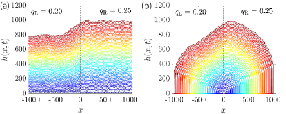
Typical height profiles for the flat and droplet cases are shown in Fig. 2. In the flat case, the interface consists of two flat regions growing at different speeds, connected by a slope near the boundary [Fig. 2(a)]. Interestingly, the slope is found to be kept constant in time, though the difference between the heights far from the boundary increases. This can be understood by considering the noiseless version of the KPZ equation:

$$\begin{cases}\frac{\partial h}{\partial t}=\nu\frac{\partial^{2}h}{\partial{x}^{2}}+\frac{\lambda}{2}\left(\frac{\partial h}{\partial x}\right)^{2}+v_{\mathrm{L}},&(x<0),\\ \frac{\partial h}{\partial t}=\nu\frac{\partial^{2}h}{\partial{x}^{2}}+\frac{\lambda}{2}\left(\frac{\partial h}{\partial x}\right)^{2}+v_{\mathrm{R}},&(x\geq 0),\end{cases}$$ (8)

where $\nu$ and $\lambda$ are constant coefficients and $v_{\mathrm{L}}<v_{\mathrm{R}}$ denote the two growth speeds. The asymptotic solution $h_{\mathrm{asymp}}(x,t)$ is

$$h_{\mathrm{asymp}}(x,t)=\begin{cases}v_{\mathrm{R}}t+\sqrt{\frac{2\Delta v}{\lambda}}x,&(x<0),\\ v_{\mathrm{R}}t+\frac{2\nu}{\lambda}\log\left(1+\frac{\lambda}{2\nu}\sqrt{\frac{2\Delta v}{\lambda}}x\right),&(x\geq 0),\end{cases}$$ (9)

with $\Delta{}v:={}v_{\mathrm{R}}-v_{\mathrm{L}}$. This accounts for the numerically observed appearance of the constant slope, which penetrates into the faster-growth region over a finite distance.

In the droplet case, the asymptotic mean profile in the homogeneous growth condition $q_{\mathrm{L}}=q_{\mathrm{R}}=q$ is known to be Sasamoto and Imamura (2004); Rost (1981)

$$h(x,t)\simeq v_{\infty}t\frac{\sqrt{q}+\sqrt{1-(x/t)^{2}}}{1+\sqrt{q}},$$ (10)

i.e., an expanding semicircle with a rising center. Then, in our biregional setting $q_{\mathrm{L}}<q_{\mathrm{R}}$, if there were no interaction between the two regions, two quadrants of different radii would grow. However, the same sort of interaction as for the flat case exists, producing a similar intermediate region of a constant slope [Fig. 2(b)].

III.2 Distribution at the Boundary

Now we study how the interface fluctuates around the mean profile, at and near the boundary. The result of the mean height profile, in particular Eq. (9), suggests that this boundary region is essentially controlled by the faster-growth region. Therefore, the height should be rescaled by Eq. (5) with Eq. (4) and $q=q_{\mathrm{R}}=0.25$; specifically, $v_{\infty}=1,\,\Gamma=3,\,c=3^{-2/3}$. In this section, we study the rescaled height fluctuations at the boundary, $H(0,t)$.

Figure 3: The mean and the variance of the rescaled height $H(0,t)$ at the boundary for the droplet case. Different colors and symbols correspond to different values of $q_{\mathrm{L}}$, as shown in the legend of panel (c). The horizontal lines indicate the mean and the variance of $\chi_{\mathrm{GUE}}$ (dashed) and $\chi_{\mathrm{GSE}}^{\prime}$ (dash-dot). The raw data in (a)(b) are plotted against $(\Delta{}q)^{3/2}t$ in (c)(d). The insets show approach to the GSE-TW values. To improve statistical accuracy, the data for $q_{\mathrm{L}}=0.240$ were obtained from 500,000 realizations. In view of the alternating character of the updating, only data at even times are shown.

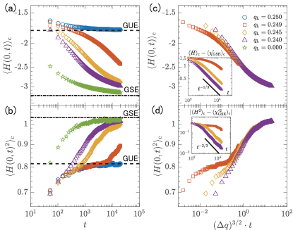
First, the results for the droplet case are shown in Fig. 3. Figures 3(a) and (b) show the mean $\braket{H(0,t)}$ and the variance $\braket{H(0,t)^{2}}_{\mathrm{c}}$, respectively, with varying $q_{\mathrm{L}}$. For the two limiting cases discussed in Sec. II.4, i.e., for the homogeneous case $q_{\mathrm{L}}=q_{\mathrm{R}}=0.250$ (blue circles) and the half-space case $q_{\mathrm{L}}=0$ (green stars), our numerical data support the expected convergence to the GUE-TW and GSE-TW distributions, respectively [Eqs. (6) and (7)]. The data in between correspond to the results of our biregional setting, which seem to approach the GSE-TW values asymptotically. Indeed, by plotting the difference from the GSE-TW values against $t$ [Fig. 3(c)(d) insets], we find $\braket{H(0,t)}\to\braket{\chi_{\mathrm{GSE}}^{\prime}}$ and $\braket{H(0,t)^{2}}_{\mathrm{c}}\to\braket{\chi_{\mathrm{GSE}}^{\prime 2}}_{\mathrm{c}}$ with finite-time corrections $\sim{}t^{-1/3}$ and $t^{-2/3}$, respectively.

Moreover, if $q_{\mathrm{L}}$ is sufficiently close to $q_{\mathrm{R}}$ [e.g., red squares in Fig. 3(a)(b)], the data first stay near the curve for $q_{\mathrm{L}}=q_{\mathrm{R}}$, during which the distribution is essentially GUE-TW (plus finite-time corrections), then crossover to the GSE-TW values. To characterize this crossover, we tried to collapse the data in Fig. 3(a)(b) by rescaling the abscissa in the form $(\Delta{}q)^{\mu}t$, with $\Delta{}q:=q_{\mathrm{R}}-q_{\mathrm{L}}$ and some exponent $\mu$. The best collapse was achieved with $\mu=1.4\pm 0.1$. From the theoretical viewpoint, it is reasonable to assume that this crossover occurs when the height difference induced by the two different growth speeds, $\Delta{}vt\sim\Delta{}qt$, becomes comparable to the fluctuation amplitude $(\Gamma{}t)^{1/3}$. This gives $t\sim(\Delta{}q)^{-3/2}$, hence $\mu=3/2$. Our data are indeed consistent with this value [Fig. 3(c)(d)].

Figure 4: The mean and the variance of the rescaled height $H(0,t)$ at the boundary for the flat case. The horizontal lines indicate the mean and the variance of $\chi_{\mathrm{GOE}}^{\prime}$ (dashed) and $\chi_{\mathrm{GUE}}$ (dash-dot).

Figure 5: The mean and the variance of the rescaled height $H(0,t)$ at the boundary for the stationary case. The horizontal lines indicate the mean and the variance of $\chi_{\mathrm{BR}}$ (dashed) and $\chi_{\mathrm{GOE}}$ (dash-dot).

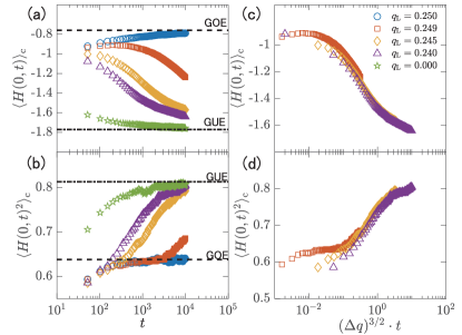
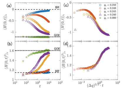
We also studied the flat and stationary cases and reached analogous conclusions: for the flat case (Fig. 4) we find crossover from the GOE-TW to GUE-TW distributions, and for the stationary case (Fig. 5) from BR to GOE-TW [recall the limiting cases, Eqs. (6) and (7)]. The data are found to be consistent with the same crossover exponent $\mu=3/2$.

III.3 Distribution near the Boundary

Figure 6: The mean and the variance of the compensated rescaled height $\tilde{H}(X,t)$ near the boundary for the droplet case. The dashed lines indicate the theoretical curves for the half-space KPZ (Theorem 5.3 of Ref.Sasamoto and Imamura (2004)), numerically evaluated by J. De Nardis and P. Le Doussal.

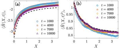
Here we report briefly on the one-point distribution near the boundary, $X>0$. In the case of the half-space droplet PNG without boundary nucleation, Sasamoto and Imamura Sasamoto and Imamura (2004) derived a formula (their Theorem 5.3) for the multiple-point joint distribution of the rescaled height $H(X,\infty)$, or more precisely, $H(X,\infty)+X^{2}$ to compensate the parabolic shape near the top of the droplet [see Eq. (6)]. Since this formula also contains information of the one-point distribution near the boundary, we aim to compare it with our numerical data. To do so with data obtained at finite times, we need to compensate not only the parabolic term, but also higher-order nonlinearities due to the global semicircle shape of the droplet [Eq. (10)]. This led us to define the compensated rescaled height by

$$\tilde{H}(X,t) :=H(X,t)+\frac{v_{\infty}t}{(1+\sqrt{q})(\Gamma t)^{1/3}}\left[1-\sqrt{1-(x/t)^{2}}\right]$$

$$\simeq H(X,t)+X^{2}.$$ (11)

Figure 6 shows the mean and the variance of $\tilde{H}(X,t)$ with $q_{\mathrm{L}}=0$ (colored symbols), compared with the predictions from Sasamoto and Imamura’s formula (dashed lines). The results for the variance are found to agree with the theoretical curve [Fig. 6(b)], but finite-time corrections are also seen. Convergence is unfortunately slower for the mean [Fig. 6(a)], still unreached at the largest time we used. For the biregional case $q_{\mathrm{L}}>0$, given the result of the crossover time $\sim(\Delta{}q)^{-3/2}$, convergence to such asymptotic behavior will be even slower. However, Fig. 6 nicely illustrates that the one-point distribution in the droplet case crossovers from the GSE-TW statistics at the origin to the GUE-TW one in the bulk (far from the boundary). Analogous crossover, from GUE-TW to GOE-TW for the flat case and from GOE-TW to BR for the stationary case, is also expected.

III.4 Spatial Correlation

Figure 7: The rescaled spatial correlation function $C_{\mathrm{s}}^{\prime}(X,t)$ for the droplet (a-c) and the flat (d-f) cases. In (a,d), $t$ is fixed ($t=10000$) and $q_{\mathrm{L}}$ is varied. In (b,e), $q_{\mathrm{L}}$ is fixed ($q_{\mathrm{L}}=0.246$) and $t$ is varied. In (c,f), pairs of $q_{\mathrm{L}}$ and $t$ that give the same value of $(\Delta q)^{3/2}t$ are used. The panel (g) shows the asymptotic forms of the correlation function for the half-space problem, compared with the Airy₁ and Airy₂ correlation for the full-space problem. The curves for the Airy₂ and Airy₁ processes were numerically evaluated by F. Bornemann Bornemann (2010).

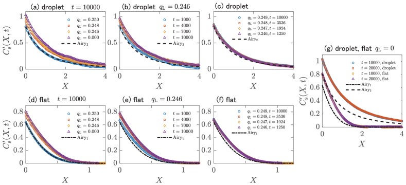
Finally we study the two-point spatial correlation function, defined by

$$C_{\mathrm{s}}(x,t):=\braket{h(x,t)h(0,t)}-\braket{h(x,t)}\braket{h(0,t)}$$ (12)

and rescaled as $C^{\prime}_{\mathrm{s}}(X,t):=C_{\mathrm{s}}(x=Xt^{2/3}/c,t)/(\Gamma t)^{2/3}$. For the homogeneous growth $q_{\mathrm{L}}=q_{\mathrm{R}}$, it is known that the asymptotic spatial profile is given by the stochastic process called the Airy₂ process for the droplet case Prähofer and Spohn (2002b) and the Airy₁ process for the flat case Sasamoto (2005). Therefore, the spatial correlation function $C^{\prime}_{\mathrm{s}}(X,t)$ is given directly by their time correlation, for which analytical formulae are known Prähofer and Spohn (2002b); Sasamoto (2005). For the half-space droplet case ($q_{\mathrm{L}}=0$), Sasamoto and Imamura’s formula Sasamoto and Imamura (2004) describes this correlation.

Figure 7 shows our numerical results. For the droplet case, $C^{\prime}_{\mathrm{s}}(X,t)$ is plotted in Fig. 7(a) with fixed $t$ and varying $q_{\mathrm{L}}$. We can confirm that the data for $q_{\mathrm{L}}=q_{\mathrm{R}}=0.250$ are in agreement with the Airy₂ correlation (dashed line). The corresponding formula by Sasamoto and Imamura is yet to be evaluated, but since our model with $q_{\mathrm{L}}=0$ is equivalent to the half-space PNG studied by them, we expect that our data show the functional form of their formula [top data set in Fig. 7(g)]. For the biregional case $0<q_{\mathrm{L}}<q_{\mathrm{R}}$, we see the data crossover from Airy₂ to the half-space result, with increasing $\Delta{}q$ (decreasing $q_{\mathrm{L}}$) [Fig. 7(a)] or increasing $t$ (with fixed $\Delta{}q$) [Fig. 7(b)]. This crossover is again controlled by the rescaled time $(\Delta{}q)^{3/2}t$, which is confirmed in Fig. 7(c) by plotting $C^{\prime}_{\mathrm{s}}(X,t)$ for several pairs of $q_{\mathrm{L}}$ and $t$ that give the same value of $(\Delta q)^{3/2}t$. We also tried data collapse of $C^{\prime}_{\mathrm{s}}(X,t)$ assuming the combination $(\Delta q)^{\mu}t$ with parameter $\mu$. It was a difficult task due to unavoidable influence from finite-time effect and statistical error, but we obtained $\mu=1.3\pm 0.2$, in reasonable agreement with $\mu=3/2$ expected from the theoretical argument described in Sec. III.2.

The same analysis is carried out in Fig. 7(d-f) for the flat case. We observe analogous crossover from the Airy₁ correlation (dash-dot lines) to the correlation expected to be that of the half-space flat KPZ problem [purple triangles in Fig. 7(d) or bottom data set in Fig. 7(g)]. To our knowledge, the latter correlation has not been studied theoretically.

IV concluding remarks

In this paper, we have proposed a new “biregional” situation for studying the KPZ class, where the interface grows at different speeds in the left and right halves of space. We have implemented it using the discrete PNG model for the three representative geometries, namely the droplet, flat, and stationary cases, and numerically studied the fluctuation properties at and near the boundary. As a result, we have found that they are asymptotically well described by the half-space problem of the KPZ class, which is characterized by the sets of the universal statistical properties different from those for the homogeneous, full-space problem. In particular, the GSE-TW distribution was found for the biregional droplet case. If the growth speed difference is small, we have found crossover from the full-space statistics to the half-space one, which is controlled by the rescaled time $(\Delta{}v)^{3/2}t$ with growth-speed difference $\Delta v$.

Our result may also be interpreted in terms of the directed polymer in random medium, which provides one of the standard representations of the KPZ class Kriecherbauer and Krug (2010); Corwin (2012); Halpin-Healy and Takeuchi (2015); Takeuchi (2017). In the translation from interface to directed polymer, growth speed corresponds to the mean depth of the random potential and the height to the free energy of the polymer, which tends to find the optimal path under a given random potential. Now, in our biregional setting, the mean depth of the potential is different between the two regions. If this gap is large enough, the optimal path is expected to be found essentially inside the deeper half space. The correspondence to the half-space problem is reasonable from this viewpoint. It is also interesting to recall our finding that the mean interface profile develops a constant slope near the boundary. In this sense, a situation similar to imposing the Neumann boundary condition is spontaneously realized in our setting, providing another explanation on the correspondence to the half-space problem. In any case, carrying out direct theoretical analysis of the biregional KPZ problem is an interesting open problem left for future studies.

Finally, we believe that our biregional setting has strong experimental relevance, compared with the standard half-space problem for which the boundary condition needs to be controlled. A study using the liquid-crystal turbulence Takeuchi and Sano (2010) is ongoing. We also consider that a similar situation can be realized in other experimental systems showing KPZ, such as mutant bacteria colonies Wakita et al. (1997) and paper combustion Maunuksela et al. (1997); *Myllys.etal-PRE2001. We hope the biregional setting will be a useful platform to investigate the KPZ half-space problem, both theoretically and experimentally.