Weak lensing Study in VOICE Survey I: Shear Measurement

Abstract

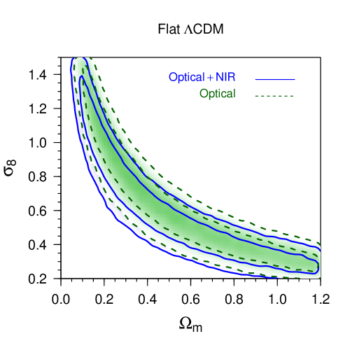
The VST Optical Imaging of the CDFS and ES1 Fields (VOICE) Survey is a Guaranteed Time program carried out with the ESO/VST telescope to provide deep optical imaging over two 4 deg² patches of the sky centred on the CDFS and ES1 pointings. We present the cosmic shear measurement over the 4 deg² covering the CDFS region in the $r$-band using LensFit. Each of the four tiles of 1 deg² has more than one hundred exposures, of which more than 50 exposures passed a series of image quality selection criteria for weak lensing study. The $5\sigma$ limiting magnitude in $r$- band is 26.1 for point sources, which is $\begin{array}[]{c}>\\ \sim\end{array}1$ mag deeper than other weak lensing survey in the literature (e.g. the Kilo Degree Survey, KiDS, at VST). The photometric redshifts are estimated using the VOICE $u,g,r,i$ together with near-infrared VIDEO data $Y,J,H,K_{s}$. The mean redshift of the shear catalogue is 0.87, considering the shear weight. The effective galaxy number density is 16.35 gal/arcmin², which is nearly twice the one of KiDS. The performance of LensFit on such a deep dataset was calibrated using VOICE-like mock image simulations. Furthermore, we have analyzed the reliability of the shear catalogue by calculating the star-galaxy cross-correlations, the tomographic shear correlations of two redshift bins and the contaminations of the blended galaxies. As a further sanity check, we have constrained cosmological parameters by exploring the parameter space with Population Monte Carlo sampling. For a flat $\Lambda$CDM model we have obtained $\Sigma_{8}=\sigma_{8}(\Omega_{\rm m}/0.3)^{0.5}=0.68^{+0.11}_{-0.15}$.

1 Introduction

Gravitational lensing is the image distortion of background galaxies (sources) due to the differential deflection of their light caused by foreground masses (lenses). The induced coherent shape distortion of source images is referred to as weak lensing shear, and it is typically much smaller than the intrinsic ellipticity of the source galaxies. Such signals can only be measured in a statistical way by averaging over a large sample of galaxies. Weak lensing effects depend sensitively on the growth of large-scale structures and the expansion history of the Universe, thus representing a probe complementary to other observables in order to constrain cosmological models (e.g. Hinshaw et al., 2013; Planck Collaboration et al., 2016). Furthermore, the gravitational nature of weak lensing makes this effect particularly important in probing the dark side of the Universe (e.g. Bartelmann & Schneider, 2001; Fu & Fan, 2014; Kilbinger, 2015; Mandelbaum, 2017).

The progresses of cosmological studies based on weak lensing rely on the developments of wide-field imaging surveys. The Canada-France-Hawaii Telescope Lensing Survey (CFHTLenS, Heymans et al., 2012a) has shown that cosmic shear is a powerful cosmological probe (Kilbinger et al., 2013; Benjamin et al., 2013; Fu et al., 2014; Liu et al., 2016). On-going surveys, such as the Dark Energy Survey (DES, Becker et al., 2016; Jarvis et al., 2016), the Kilo-Degree Survey (KiDS, Kuijken et al., 2015; Hildebrandt et al., 2017) and the Hyper Suprime-Cam (HSC) survey (Aihara et al., 2018; Mandelbaum et al., 2018) are enlarging the sky coverage to a few thousands square degrees. In the coming years, next-generation weak-lensing projects such as the Euclid mission, the wide Field Infrared Survey Telescope (WFIRST) and the Large Synoptic Survey Telescope (LSST) will produce a large breakthrough in survey volume and depth, making high-precision weak lensing studies possible.

While the large-sky coverage is essential to minimize the cosmic variance, the survey depth of weak lensing surveys is crucial to study the evolution of large-scale structures over the widest redshift range. However, deep imaging surveys present different challenges. The higher number density of background galaxy (few tens to hundred galaxies per square arcminute) causes crowding problems, making object de-blending a serious issue, particularly for ground-based observations. Moreover, due to the more stringent observing conditions, deep surveys for weak lensing are more difficult to plan and carry-out, compared to wide surveys. Despite that, there are a number of deep small sized surveys which have set the ground in the field. CFHTLS Deep (Semboloni et al., 2006) has been the first generation of these deep surveys, and released a 4 deg² shear catalogue with the depth of $i=25.5$. More recently, the Deep Lens Survey (DLS, Jee et al., 2013, 2016) successfully derived cosmological constraints using a cosmic shear catalogue with a limit of $r=27$ mag and a mean source redshift of $z_{s}\sim 1$ over 20 deg². Schrabback et al. (2010) presented the space-based galaxy shape measurements Hubble Space Telescope Cosmic Evolution Survey (COSMOS) and found evidence of the accelerated expansion of the Universe from weak lensing tomography. This result has been obtained with data collected over a field of view of only 1.64 deg², but with a very high galaxy number density, 76 arcmin^-2 with limiting magnitude $i<26.7$ mag.

The VLT Survey Telescope (VST) Optical Imaging of CDFS and ES1 (VOICE, co-PIs: Giovanni Covone & Mattia Vaccari, Vaccari et al., 2016) is a Guaranteed Time of Observation (GTO) survey preformed with the ESO/VST telescope (Capaccioli & Schipani 2011) operating on Cerro Paranal (Chile). VOICE shared observations with the SUpernova Diversity And Rate Evolution (SUDARE), another VST GTO survey, to cover the CDFS sky region (Cappellaro et al., 2015; Botticella et al., 2017). SUDARE has observed the common fields in the $g,r,i$, optimizing the strategy in order to search and characterize supernovae at intermediate redshift ($0.3\begin{array}[]{c}<\\ \sim\end{array}z\begin{array}[]{c}<\\ \sim\end{array}0.6$). The VOICE team has been in charge of the $u$ band observations of the same area. For their science case, SUDARE required less stringent constraints on image quality, however the number of epochs was so large that the total amount of data with image quality within VOICE specs in $g,r,i$ allowed us to reach the necessary depth in the stacked images required by the VOICE science objectives, including weak lensing.

The two selected fields, VOICE-CDFS and VOICE-ES1, have been also observed by other facilities on a wide wavelength range, including GALEX (UV), VISTA-VIDEO (NIR), Spitzer-SERVS (MIR), Herschel-HerME (FIR), Spitzer SWIRE (IR), and ATLAS (radio). Adding optical data from VOICE has made these fields extremely valuable for a large range of astrophysical studies. One of the science drivers for VOICE is to detect clusters of galaxies at relatively high redshifts, and to study their mass distributions using weak lensing signals of galaxies in the fields.

The VOICE survey uses the same telescope, detector (OmegaCAM) and optical filters as KiDS. The $r$-band data are used for weak lensing measurements. Differently from KiDS, where each pointing is observed only in one epoch consisting of five consecutive exposures, the VOICE survey holds multiple-epoch observations for each pointing of the $r$-band with total number of exposures over a hundred. For the data used for weak lensing shear measurements, the $5\sigma$ limiting magnitude for point source in $r$-band co-added images reaches $r=26.1$ mag within 2″aperture diameter, which is about $1.2$ magnitude deeper than KiDS data.

As in KiDS (Kuijken et al., 2015, hereafter K15), we used LensFit (Miller et al., 2007; Kitching et al., 2008; Miller et al., 2013) to measure the galaxy shapes. To this end, some preliminary steps were required. First, the observing conditions varied significantly from epoch to epoch and we needed to go through a severe quality control of the individual exposures. Second, we needed to adapt the LensFit parameters for our dataset, since VOICE data are deeper than CFHTLenS and KiDS (de Jong et al., 2017). To validate the setup and calibrate the shear measurement, we made use of dedicated simulations which have been presented in a companion paper Liu et al. (2018).

The structure of this paper is organized as follows. In Section 2, we describe VOICE data and data reduction. The shape measurement procedures, the calibration from VOICE-like simulation and the photometric redshift are presented in Section 3. Two-point correlation analyses and null tests for shear systematics are presented in Section 4. To further demonstrate the quality of our shear measurements, in Section 5, we show the cosmological constraints of $\Omega_{\rm m}$ and $\sigma_{8}$ derived from cosmic shear two-point correlations. The summary is given in Section 6.

2 The survey

This paper focuses on the VOICE-CDFS field, which covers about 4.9 deg². It is composed by four tiles (CDFS1, CDFS2, CDFS3, CDFS4), about 1 deg² each. The pixel scale of the OmegaCAM CCDs is $0.21^{\prime\prime}$. The center of the VOICE-CDFS field is RA$=03^{\rm h}32^{\rm m}30^{\rm s}$ and DEC$=-27^{o}48\arcmin 30\arcsec$. The observations started in October 2011, and ended in 2015. Each tile was observed in four optical bands $u,g,r,i$ with exposure time of 600s ($u$), 360s ($g$ and $r$) and 400s ($i$), respectively. The $r$-band data were used, in addition to the weak lensing study presented here, for variability based search of supernovae (Botticella et al., 2017) and Active Galactic Nuclei (Falocco et al., 2015; De Cicco et al., 2015). For each tile, more than one hundred exposures were taken in the $r$-band. As in KiDS, a single epoch consists of five consecutive exposures obtained with a diagonal dithering pattern to cover the detector gaps. The initial position and the dithering pattern is repeated at any epoch. The cumulative exposure time ranges from 15.3 to 20.9 hours for the four fields. The total exposure time for the other three bands is shorter as shown in Table 1. As $\sim 100$ VOICE exposures are distributed over four years, the image quality and the point spread function (PSF) of the individual exposures varies significantly in exposures from different epochs.

Table 1: The total exposure time (in hours) of four VOICE-CDFS fields in the $u,g,r,i$ bands before applying any image quality selections (Sect. 2.1).

	$u$	$g$	$r$	$i$
CDFS1	5.20	5.64	20.90	8.41
CDFS2	6.50	4.83	15.30	4.38
CDFS3	0.83	6.94	20.60	9.47
CDFS4	0.83	5.43	18.50	8.51

2.1 Exposure selections

The data reduction was performed using the pipeline VST-Tube (Grado et al., 2012). As described in detail in Cappellaro et al. (2015), VST-Tube performs over scan correction, flat fielding, CCD gain harmonization, illumination correction, and cosmic ray removal.

Since the shear signal is very weak, about an order of magnitude smaller than the intrinsic ellipticity of galaxies, we have applied very strict image selection criteria. VOICE $r$-band observations were carried out over 4 years, therefore, the observing conditions show significant variations among epochs. In order to obtain an homogeous dataset and maximize the quality of our shear measurements, we have filtered our data according to seeing and its variations within the field of view before further data processing (i.e., image co-adding, object detection and shape measurements).

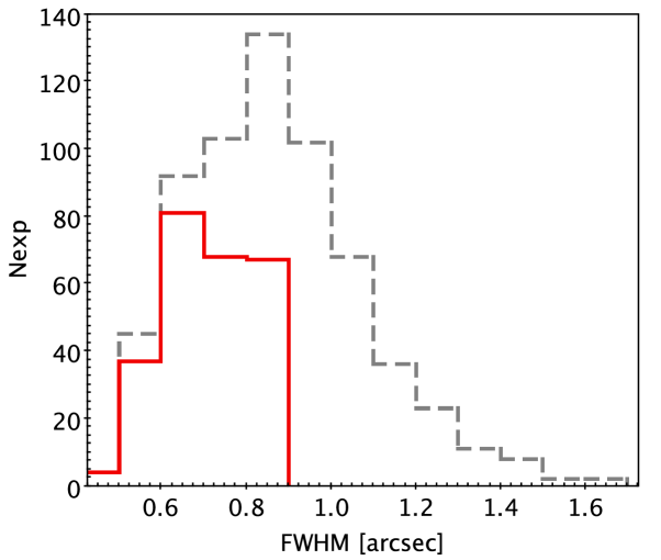
The PSF full width at half maximum (FWHM) of different exposures in the $r$-band ranges from 0.4$\arcsec$ to 1.5$\arcsec$ as shown in the top panel of Fig. 1. The median value is 0.86$\arcsec$. Weak lensing studies focus on background galaxies which are mostly faint and small. Because seeing smears galaxy images if they are significantly smaller than the seeing disc, we have selected only those exposures with seeing smaller than $0.9\arcsec$.

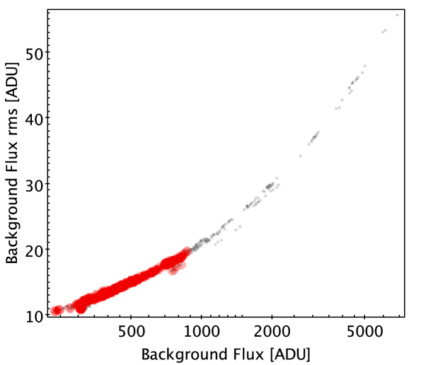
The sky background brightness can also affect object detection and shape measurement. The background values calculated by SExtractor (Bertin, 2011) spread in an extremely wide range, from a few hundreds to a few thousands Analog-to-Digital Units (ADUs). We assigned the median background value of the 32 CCDs as the reference background flux value of each exposure. As shown in the bottom panel of Fig. 1, the rms value is strongly correlated with the background flux. Most of the exposures showed relatively small background flux and small variations from CCD to CCD. We have then applied a cut on the background rms dispersion in order to have a homogeneous background noise. After several iterations examining the B-mode in the shear two-point correlations, the exposures with background rms dispersion over 20 were rejected in the shear analysis, corresponding to a background flux cut of $<\sim$900 ADU.

In order to have a uniform depth from epoch to epoch, we further reviewed the remaining exposures, and only kept those epochs with at least four exposures passing the selection criteria. In conclusion, about one-third of total exposures were used for weak lensing analysis, as shown in red in Fig. 1. The number of useful exposures for the four tiles is 62, 54, 79 and 62, respectively. The final mosaic reaches a 5$\sigma$ limiting magnitude of $r_{\rm AB}=26.1$ within 2$\arcsec$ aperture diameter for point sources. The average limiting magnitude for $u,g,i$ bands is 25.3, 26.4, 25.2, respectively.

2.2 Astrometric calibration

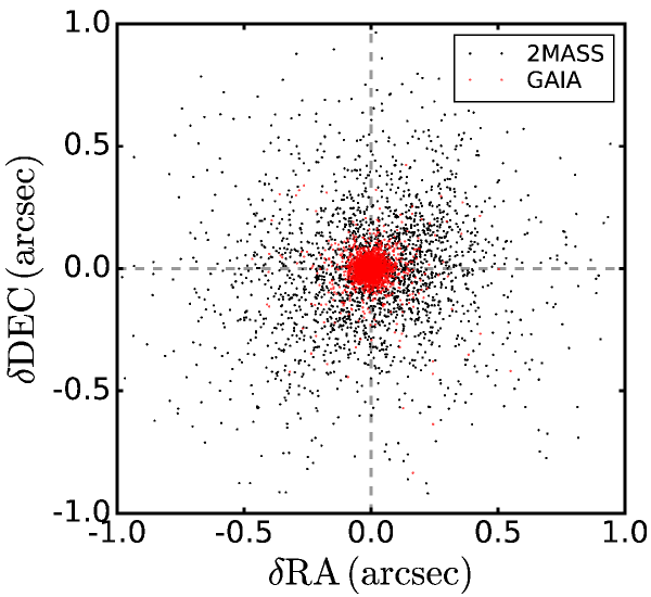
The astrometric calibration of each tile has been performed separately using the software SCAMP. Only exposures that passed our selection criteria were used simultaneously for the calibration in order to improve the internal accuracy. The external accuracy depends on the choice of reference catalogue. We performed two sets of calibrations using 2MASS (Skrutskie et al., 2006) and GAIA (Gaia Collaboration et al., 2016), respectively. The calibrated exposures were co-added by SWarp to produce the final stacked image used for source detection. We have matched the objects between the reference catalogue and the VOICE deep image: the matched objects are 6634 and 10555 for 2MASS and GAIA, respectively. As shown in Fig. 2, the astrometric dispersion based on GAIA (0.056$\arcsec$) is about four times smaller than that from 2MASS (0.19$\arcsec$), since GAIA has smaller intrinsic astrometric uncertainties and a higher matched number of stars with respect to 2MASS. Therefore, we have chosen GAIA as the absolute reference for the VOICE astrometric calibration.

Figure 1: The PSF FWHM distribution (top) and the correlation between background value and its CCD to CCD dispersion (bottom) of all $r$-band exposures (grey). The final selected exposures are shown in red.

Figure 2: The RA and Dec difference of matched objects between VOICE and 2MASS (black), or VOICE and GAIA (red).

Figure 3: Example of Masked regions covering saturated stars, halos, spikes and the other defects in the CDFS2.

Table 2: The number of sources used in our analysis in the four CDFS tiles in the $r$-band: $\rm N_{star}$ is the number of stars used for PSF correction; $\rm N_{\rm gal}$ is the number of galaxies detected from the co-added deep image; $\rm N_{\rm shear}$ is the number of galaxies with LensFit non-zero weight; $\rm N_{\rm exclude}$ is the number of galaxies excluded before model fitting; $\rm N_{\rm wzero}$ is the number of galaxies that passed exclusion selection but failed in LensFit model fitting with zero weight.

	CDFS1	CDFS2	CDFS3	CDFS4
$\rm N_{star}$	2878	2807	2851	2774
$\rm N_{\rm gal}$	129505	125032	126360	125295
$\rm N_{\rm shear}$	84406	83425	78445	77499
$\rm N_{\rm exclude}$	24686	22946	25830	23914
$\rm N_{\rm wzero}$	20413	18661	22085	23882

2.3 Mask

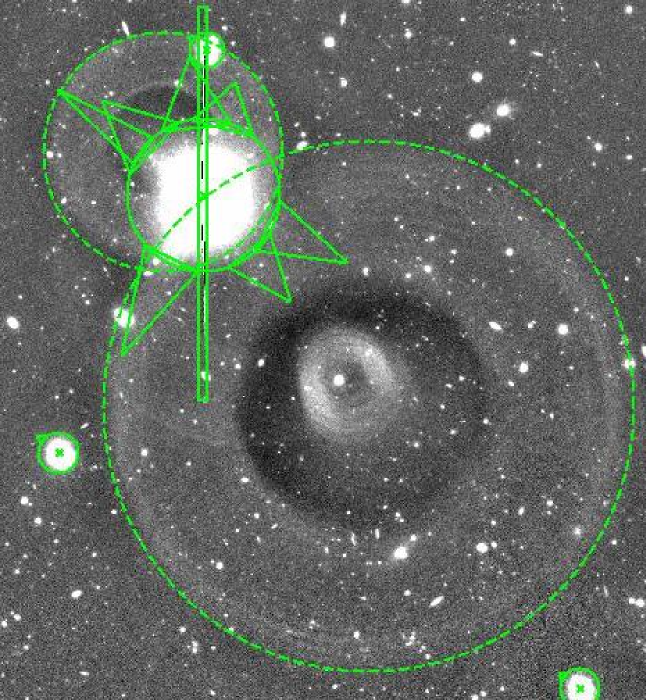
Saturated stars and their surrounding areas have to be masked because the flux measured in those regions can be affected by strong systematic errors. Those areas were identified by the automatic mask software Pullecenella (Huang et al., 2011; de Jong et al., 2015), which has been created specifically to treat the VST images. For LensFit, the galaxy model fitting is performed on each individual exposure. Thus the masks were not produced from the deep co-added images in order to avoid over masking. Instead, we masked the affected areas of the individual epochs, i.e., the stacked images over five consecutive and dithered exposures. Fig. 3 shows an example of masked regions near saturated stars with a large reflection halo. The remaining unaffected area after masking is $\sim$ 84% of the original 4.9 deg² VOICE-CDFS area.

2.4 Photometric redshift catalogue description

For each tile all the high-quality, astrometric calibrated exposures were co-added using SWarp to produce the deep stacked image. Source positions and star-galaxy classification were performed on the stacked image. The SExtractor software (Bertin & Arnouts, 1996) was run to generate the final source catalogue. The star-galaxy classification was done in the magnitude-size diagram (Huang et al., 2011), where magnitude and size are represented by the SExtractor parameters MAG_AUTO and MU_MAG$-$MAG_AUTO. Sources with size smaller than the stellar one were defined as spurious and removed from the catalogue. As shown in Table 2, about 2800 stars were selected from each tile and used to measure the PSF. More than $1.25\times 10^{5}$ galaxies per tile were selected. This galaxy catalogue was used for the photometric redshift estimates (photo-$z$) and also as input to the shape measurement software LensFit (Miller et al., 2007; Kitching et al., 2008; Miller et al., 2013).

For photo-$z$ measurements, we employed the optical observations in $u,g,r,i$ from VOICE, and the near-infrared $Y,J,H,K_{s}$ data obtained by the VIDEO survey (Jarvis et al., 2013) performed with the VISTA telescope. The NIR bands cover $>$ 80% of the VOICE images. We did not include the VIDEO $Z$ band since it covers a negligible fraction ($<$ 50%) of the VOICE area. The VOICE and VIDEO stacks were produced selecting exposures with a similar cut in the seeing ($\leq$ 1.0 arcsec). We therefore decided to base our photometric redshift estimate on magnitudes measured on apertures of the same size in all bands. To this end we used the SEP Python library (Barbary, 2016): the SEP library implements algorithms from the SExtractor software (Bertin & Arnouts, 1996) as stand-alone functions and classes. We used it to measure $u,g,r,i,Y,J,H,K_{s}$ aperture magnitudes (6$\arcsec$ diameters) centered on the source positions in the $r$-band catalogue. Compared to the so-called dual-mode in SExtractor, the SEP library allows to perform a list-driven photometry on images with different size, scale or center: WCS coordinates from the catalogue were converted to pixel positions in the image using functions available in the astropy python library and then passed to SEP. Background subtraction is also available within SEP.

The next step was the removal of residual errors in the calibration of the photometric zero point. To this end, we benefit from the overlap of the CDFS fields with the APASS survey. We matched $\sim 200$ unsaturated stars (15 $<r<$16 ) in the $gri$. Non-negligible offsets ($<0.1$ mag) were found in $g$ (CDFS3 and CDSF4) and $i$ (CDFS3).

Photo-$z$ were finally derived using the BPZ software (Benítez, 2011): BPZ adopts a Bayesian approach, where the likelihood that a template fits the colours of a galaxy at a given redshift is combined with a prior defining the probability to find a galaxy of that type, as a function of magnitude and redshift. This allows to reject those solutions which would maximize the likelihood, but that would be unphysical according the known prior distributions. The BPZ library consists (Benítez et al., 2004) of four modified Coleman, Wu and Weedman types (Coleman et al., 1980), and two Kinney, Calzetti & Bohlin (Kinney et al., 1996) starburst galaxy templates. The derived photo-$z$ are discussed in Sect. 3.4.

Figure 4: Examples of variations in PSF patterns in VOICE-CDFS1 for four epochs observed from summer to winter.

3 LensFit Shape measurement

The shear measurement accuracy depends sensitively on the data quality and on the data processing steps, such as the observing conditions, the quality of the camera, the PSF shape and stability, the background noise, etc.. It is also crucial to use a reliable shape measurement algorithm optimized for the considered survey. Image simulations specifically made for the survey are normally needed to validate the optimizations and also to quantify the possible biases in the shear measurements.

KiDS data analyses (e.g., Hildebrandt et al., 2017) proved that LensFit (Miller et al., 2013, hereafter M13) is a suitable shape measurement algorithm for OmegaCAM images, with an accuracy reaching $\sim$1%.

We therefore also adopted LensFit for the shape measurement. LensFit constructs a seven-parameter galaxy model fit including the galaxy position, flux, scale-length, bulge-to-disc ratio, and galaxy ellipticity. Although the signal-to-noise ratio of an individual galaxy detected from co-added image is high, using the co-added image is problematic for high-precision galaxy shape measurement, mainly because the co-addition of PSFs of different shapes and orientations from different exposures may result in a complex stacked PSF. Furthermore, the co-adding procedures (particularly the interpolation of individual exposures to a common pixel grid) introduces noise correlation between pixels, which can affect the shape measurement. Thus in LensFit, the model fitting is done on individual exposures, and the probabilities of the parameters derived from different exposures for a galaxy are statistically combined to derive its final shape measurement. The details of LensFit algorithm are described in Miller et al. (2007); Kitching et al. (2008) and M13. In the following, we describe the key issues particularly relevant to the VOICE data.

3.1 PSF fitting

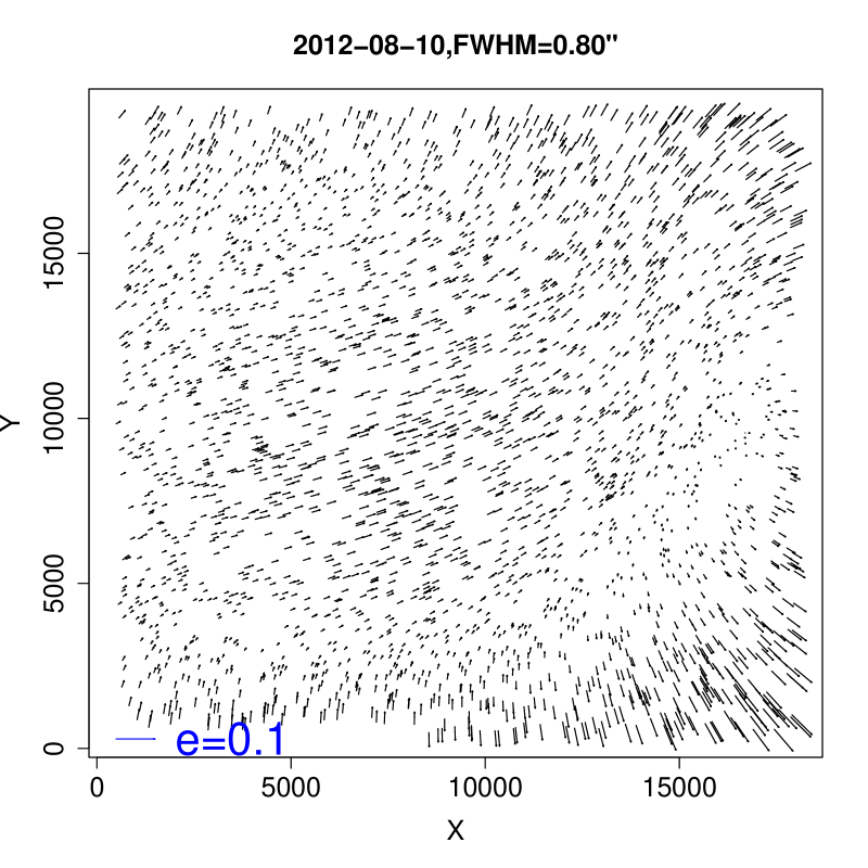
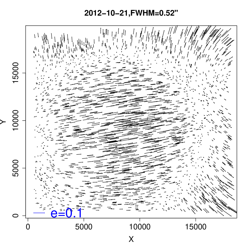
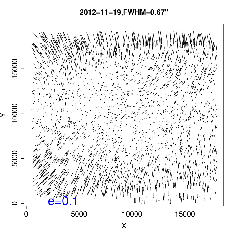
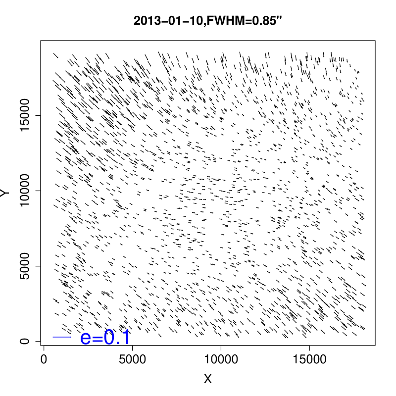
The VOICE observational campaign was distributed over several years. The PSF patterns of the same tile were very different from month to month, even night to night. We show in Fig. 4 a few examples of PSF ellipticity patterns at different epochs in the CDFS1 tile constructed by co-adding PSFs from five exposures within an epoch. The four epochs were observed at different times, from summer to winter. Strong temporal variations of PSF are clearly seen. Furthermore, any sub-optimal optical configuration of the telescope contributes significantly to the PSF. As discussed in K15, any primary mirror astigmatism of the curved focal plane of the VST results in an increasing ellipticity in the center of the field (top-right panel of Fig. 4), while a tilt of the secondary mirror causes the increase of ellipticity near one edge of the field (bottom-left panel of Fig. 4).

Therefore the PSF model fitting is made for each single exposure. Nevertheless, as shown in Fig. 4, the PSF varies not only over the full field of OmegaCAM, but also from CCD to CCD. Thus, two different polynomial fitting models were applied: a 4th order polynomial fit for the full field-of-view and a 1st order chip-dependent polynomial for individual CCDs, as done by K15 for the KiDS survey.

3.2 Exclusion of galaxies

LensFit fits each single galaxy in a postage stamp with a size of 48 $\times$ 48 pixels, which is a compromise between a stamp large enough to obtain a correct model fit, and a stamp small enough for fast processing and fitting. The center of the postage stamp was chosen to be the position of the galaxy detected from the deep co-added image. Before the model fitting, LensFit performs a few quality checks. We give a short summary here, and refer to M13 for more details about the fitting algorithm.

1. Galaxies larger than the size of the postage stamp were excluded from the analysis.
   

2. To deblend the neighboring galaxies, if more than one object is found within the same postage stamp, the algorithm checks whether the neighbour galaxy can be masked by replacing the pixel values of the background without contaminating the isophotes of the target galaxy. Comparing the Gaussian-smoothed isophotes of the neighbour galaxy measured from the co-added image to the smoothed pixel noise, if the signal-to-noise ratio is larger than a defined threshold, the neighbour galaxy will be masked out. Since VOICE is deeper than CFHTLenS and KiDS, in order to retain enough galaxies while still suppressing most of the neighbour contaminations, we optimized this threshold from two (M13 for CFHTLenS) to five. Imaging simulations of Liu et al. (2018) show that this choice does not introduce significant bias to the VOICE shear measurements. More details are discussed in Sect. 3.5 and Liu et al. (2018).
   

3. If masked pixels are outside the target galaxy’s isophote on single exposure, the pixels are replaced by the background values and the process continues. If the masked pixels are within the isophote, then that exposure will not be used in the joint analysis.
   

4. If the weighted centroid of a galaxy is more than 4 pixels away from its stamp center, it implies that there may be blended objects existed within the stamp. Thus this galaxy is excluded as well.

As shown in Table 2 (see quantity ${\rm N}_{\rm exclude}$), the fraction of excluded galaxies from the above criteria is about 19%.

3.3 Shear catalogue

Figure 5: Shear averaged weight as the function of the $r$-band galaxy magnitude.

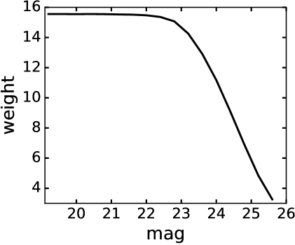
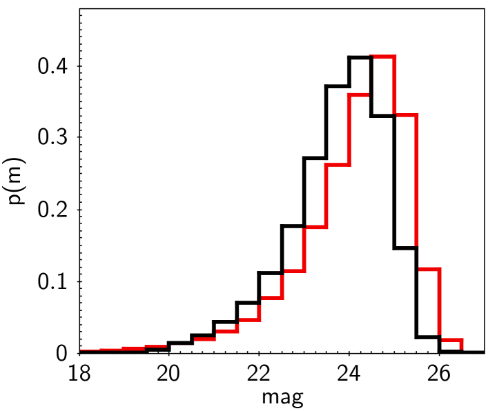
LensFit defines the galaxy weight taking into account both the shape-noise variance and ellipticity measurement-noise variance (M13). About 17% of total galaxies failed in galaxy model fitting although they passed the exclusion selection. They were given a weight of zero, and their numbers are shown as ${\rm N}_{\rm wzero}$ in Table 2. As faint galaxies are much noisier than bright ones, their weights are much lower as shown in Fig. 5. The magnitude distribution of the non-zero weight galaxies is shown in Fig. 6. The peak magnitude of the weighted distribution is about $24.2$ mag, which is about $1.0$ mag deeper than the LensFit selected galaxies in KiDS.

In order to have continuous coverage of CDFS fields, an overlap of 3$\times$7 arcmin² has been taken among the four tiles. Thus galaxies from the overlapping regions have to be dealt with separately, if they are detected more than once. Due to astrometric errors, some galaxy positions may be slightly different in the overlap region of different exposures. If a pair of galaxies has a separation of less than $3$ pixels, we considered them as a single galaxy and only kept the higher signal-to-noise measurement result.

The final shear catalogue has over $3\times 10^{5}$ galaxies with non-zero weight, corresponding to an effective weighted galaxy number density 16.35 arcmin^-2, which is about double of the density in the KiDS survey.

Figure 6: The normalized magnitude distribution of galaxies in the four CDFS fields without (red) and with (black) shear weight.

3.4 The photometric redshift distribution

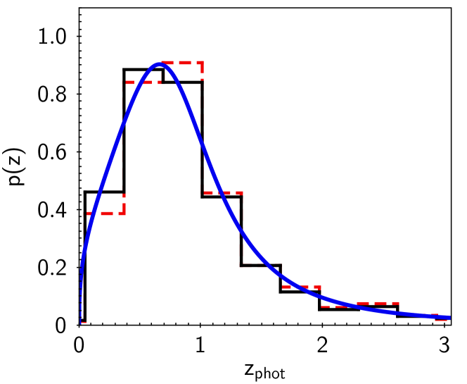
The shear catalogue was matched to the photo-$z$ catalogue (Sect. 2.4). We choose the peak value of the Probability Density Function as an estimate of its photo-$z$. The mean and median values of the photo-$z$ of the shear catalogue (non-zero weight) are 0.87 and 0.83, respectively. We fit the redshift distribution using the following formula:

$$p(z)=A\frac{z^{a}+z^{ab}}{z^{b}+c},$$ (1)

where the best fit values of the parameters $A,a,b,c$ are 0.50, 0.39, 4.66, 0.60, respectively. The histogram and the fitted photo-$z$ distributions are shown in Fig. 7. The fitted redshift distribution (Eq. 1) is used to predict the shear two-point correlation in Sect. 4.3. The normalized histogram of photo-$z$ is used for cosmological constraints (Sect. 5) to avoid the possible bias due to the model fitting.

Figure 7: The normalized distribution of photo-$z$ (peak value of PDF) of VOICE galaxies without (red dash line) and with (black solid line) shear weight. The solid blue curve is the best fit of photo-$z$ with weight.

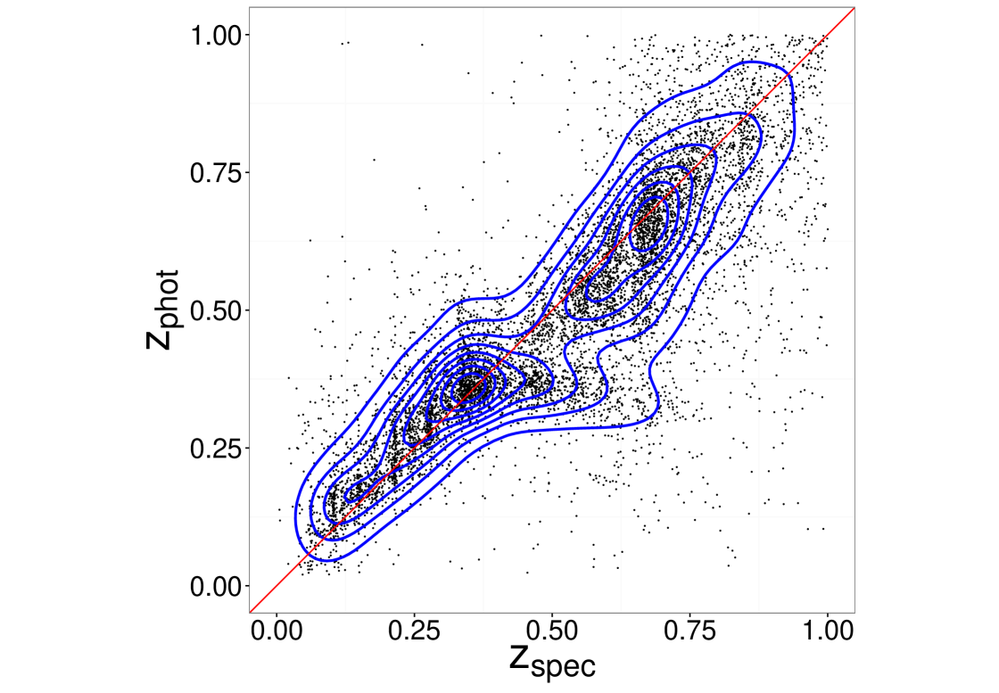
We note that this paper focuses on presenting the VOICE shear measurement results. The photo-$z$ distribution of the background galaxies are needed for cosmological constraints. We checked the photo-$z$ measurements by comparing with a subsample with spectroscopic redshifts (spec-$z$). We matched the galaxies to the spectroscopic redshift sample (Vaccari et al., 2010; Vaccari, 2015) and found 23638 galaxies. As shown in Fig. 8, the photo-$z$ has generally a good agreement with spec-$z$. The median value of $\delta z=($photo-$z-$spec-$z)/(1+$spec-$z)$ is $-0.008$ with Median Absolute Deviation (MAD) value 0.060. We separated the full sample into two redshift bins according to the median value 0.83 of the full shear catalogue. The matched galaxies in low and high bins are 19389 and 4069, respectively. The sub-samples of two redshift bins show opposite $\delta z$ as compared to the spectroscopic redshift. We found $\delta z=-0.012$ and $0.022$ for the low- and high-$z$ bin. The MAD values are 0.055 and 0.104, respectively.

Our photo-z measurements are based on the VOICE $u,g,r,i$ data together with four additional near infrared-band data $Y,J,H,K_{s}$ (8-band photo-$z$). In the appendix, we compare the photo-$z$ values withe the ones determined using only the 4 optical bands (4-band photo-$z$), to demonstrate the importance of the near–infrared bands.

Figure 8: The photo-$z$ for the galaxies of shear catalogue are matched with spectroscopic redshift sample. The contours present the density of the galaxy number.

3.5 VOICE-like simulation

VOICE is about one magnitude deeper than CFHTLenS and KiDS, composed of a few tens usable exposures for each field. We need to optimize LensFit in order to deal with the high density of background galaxies and check its capability to work with such a large number of exposures simultaneously for each galaxy shape measurement.

To validate our optimization and calibrate the measured shear, we performed image simulations representing the observed $r$-band images. We briefly summarize the simulation results here and refer to the paper by Liu et al. (2018) for more details. In the simulation, we use the sources detected in the stacked images as the input parent sample, and fix many observing conditions, such as the dithering pattern, background noise, celestial positions and brightness of the detected objects, to mimic the real observations. In this case, galaxy clustering and blending effect are included naturally. The PSFEx package (Bertin, 2011) was used to model the spatially-varing PSF for every exposure. For each galaxy, a randomly sampled intrinsic ellipticity value and a constant shear with modulus of the reduced shear $|g|$ = 0.04 was assigned. In total, four different shear combinations ($g_{1}$, $g_{2}$) were used, namely: (0.0283, 0.0283), ($-$0.0283, $-$0.0283), (0.0153, $-$0.0370), and ($-$0.0370, 0.0153), respectively. The simulated single exposure images were then generated by the Galsim toolkit (Rowe et al., 2015), and the galaxy shapes were also measured by LensFit. Overall, our simulations present good agreements with the observations, especially the distributions of the PSF properties. We applied the bin-matching method to the signal-noise-ratio (SNR) and size plane to calibrate the bias of the simulation data. The final residual multiplicative bias after calibration reaches an accuracy of 0.03 with negligible addictive bias in different SNR and size bins.

The sensitivity of the bias calibration to the undetected and neighboring objects is also discussed in Liu et al. (2018). The undetected objects are likely to skew the background noise so that they can potentially bias the shape measurements of galaxies, especially those with low SNR. Taking the depth and noise level into account, we find that the impact of the undetected galaxies is negligible for the VOICE survey. Additionally, the bias results from galaxy blending effect are also analyzed. Further analyses show that their impact on the two-point correlation function can be securely neglected due to the small fraction they account for (Sect. 4.7).

4 Shear two-point correlation analyses

Cosmic shear is the weak lensing effect caused by the large-scale structures in the Universe. We briefly summarize the theoretical relations between second-order weak lensing observables and cosmological quantities in Sect. 4.1, and then present the correlation analyses of the VOICE shear catalogue. For details on the theoretical foundation of weak gravitational lensing we refer to the literature (e.g. Bartelmann & Schneider, 2001; Fu & Fan, 2014; Kilbinger, 2015; Mandelbaum, 2017).

4.1 Theoretical background

Weak lensing induced by the large-scale structures measures the convergence power spectrum $P_{\kappa}$ through two-point correlation statistics. It is a projection of the total matter density fluctuation power spectrum $P_{\delta}$ under the Limber approximation (Kaiser, 1992):

$$P_{\kappa}(\ell)=\int_{0}^{\chi_{\rm lim}}{\mathrm{d}}\chi\,G^{2}(\chi)\,P_{\delta}\left(k=\frac{\ell}{f_{K}(\chi)};\chi\right).$$ (2)

The projection integral is carried out over the comoving distances $\chi$, from the observer out to the limiting distance $\chi_{\rm lim}$ of the survey. The lensing efficiency $G$ is given by

$$G(\chi)=\frac{3}{2}\left(\frac{H_{0}}{c}\right)^{2}\frac{\Omega_{\rm m}}{a(\chi)}\int_{\chi}^{\chi_{\rm lim}}{\mathrm{d}}\chi^{\prime}p(\chi^{\prime})\frac{f_{K}(\chi^{\prime}-\chi)}{f_{K}(\chi^{\prime})},$$ (3)

where $H_{0}$ is the Hubble constant, $c$ is the speed of light, $\Omega_{\rm m}$ is the present total matter density, and $a(\chi)$ is the scale factor at comoving distance $\chi$. The cosmology-dependent comoving angular diameter distance is denoted by $f_{K}$.

Cosmic shear two-point correlation functions (2PCFs) are the Hankel transforms of the convergence power spectrum $P_{\kappa}$, which can be written as the linear combinations of the E- and B-mode spectra, $P_{\rm E}$ and $P_{\rm B}$, respectively

$$\xi_{\pm}(\vartheta) ={1\over 2\pi}\int_{0}^{\infty}{\rm d}\ell\,\ell\,\left[P_{\rm E}(\ell)\pm P_{\rm B}(\ell)\right]{\rm J}_{0,4}(\ell\vartheta),$$ (4)

where ${\rm J}_{0}$ and ${\rm J}_{4}$ are the first-kind Bessel functions of order 0 and 4, corresponding to the components $\xi_{+}$ and $\xi_{-}$, respectively.

In real observations, the most direct measurement of weak gravitational shear signal is derived from galaxy ellipticity measurements. The unbiased 2PCFs $\xi_{+}$ and $\xi_{-}$ are estimated by averaging over pairs of galaxies (Schneider et al., 2002b),

$$\hat{\xi}_{\pm}(\vartheta)=\frac{\sum_{ij}{w_{i}w_{j}}[\epsilon_{t}(\bm{\vartheta_{i}})\epsilon_{t}(\bm{\vartheta_{j}})\pm\epsilon_{\times}(\bm{\vartheta_{i}})\epsilon_{\times}(\bm{\vartheta_{j}})]}{\sum_{ij}{w_{i}w_{j}}}.$$ (5)

Here, the sum is performed over all galaxy pairs with angular separation $\vartheta=|\bm{\vartheta}_{i}-\bm{\vartheta}_{j}|$ within some bin around $\vartheta$. $\epsilon_{t}$ and $\epsilon_{\times}$ are the tangential and cross-components of the galaxy ellipticity, respectively, with respect to the line connecting the two galaxies. $w_{i}$ is the weight for the $i$-th galaxy, obtained from the LensFit.

Assuming General Relativity, weak gravitational lensing only contributes to an E-mode power spectrum and therefore, a non-detection of the B-mode is a way to check the quality of shear measurement of the data. The E-/B-mode shear correlations $\xi_{\rm E,B}$, the aperture-mass dispersion $\langle M_{\rm ap}^{2}\rangle$ and the shear top-hat rms $\langle|\gamma|^{2}\rangle$ are the most popularly used second-order shear correlations. The decomposed E- and B-mode estimators in an aperture of radius $\theta$ can be written as integrals over the filtered correlation functions of $\xi_{+}$ and $\xi_{-}$ (Crittenden et al., 2002; Schneider et al., 2002a), as follows:

$$X_{\rm E,B}(\theta)=\frac{1}{2}\sum_{i}\vartheta_{i}\,\Delta\vartheta_{i}\left[F_{+}\left({\vartheta_{i}}\right)\xi_{+}(\vartheta_{i})\pm F_{-}\left({\vartheta_{i}}\right)\xi_{-}(\vartheta_{i})\right],$$ (6)

where $\Delta\vartheta_{i}$ is the bin width varying with $i$. The estimators $X_{\rm E}$ and $X_{\rm B}$ are only sensitive to the E- and B-mode, respectively, with suitable filter functions $F_{+}$ and $F_{-}$. The detail expressions of other two-point correlations are referred to Table 1 and Appendix A of Kilbinger et al. (2013).

4.2 Multiplicative Bias Correction

As shown in Eq. (5), given an unbiased shear measurement, 2PCFs $\xi_{+}$ and $\xi_{-}$ can be estimated, from an observational point of view, by averaging over pairs of galaxies. However, data reduction and shear measurement methods can generate possible biases. Thus a shear calibration (Heymans et al., 2012b) is usually applied to describe the relation between the observed shear and the true signal, which accounts for a potential additive bias $c_{a}$ and a multiplicative bias $m_{a}$ for the $a$-th component of the galaxy ellipticity ($a=1,2$),

$$\epsilon^{\mathrm{obs}}_{a}=(1+m_{a})\epsilon^{\mathrm{true}}_{a}+c_{a}.$$ (7)

In our analyses, the additive bias is estimated from the observational shear catalogue, and found to be consistent with zero, on average at the level of $\sim 8\times 10^{-4}$ and $\sim 3\times 10^{-5}$ for $\epsilon_{1}$ and $\epsilon_{2}$, respectively. However, the multiplicative biases are non-negligible. We derived them from on our image simulations (Liu et al., 2018). In particular, we obtained the $m$ values in multiple two-dimensional bins of the galaxy SNR and the size from simulations analysis. We then applied them to the galaxies in the observed shear catalogue according to their SNR and size. We found different values for $m_{1}$ and $m_{2}$. We then had to take into account the multiplicative bias for $\epsilon_{1}$ and $\epsilon_{2}$ separately when calculating the shear 2PCFs, which is different from previous studies, such as CFHTLenS and KiDS. We derived the corresponding 2PCFs components taking into account different $m$ values as follows.

Considering a pair of galaxies located at $\bm{\vartheta}_{i}$ and $\bm{\vartheta}_{j}$, respectively, their tangential and cross components with respect to the pair separation $\vartheta_{i}-\vartheta_{j}$ are given by

$$\epsilon_{t}=-R\mathrm{e}(\epsilon\mathrm{e}^{-2\mathrm{i}\phi});~{}~{}\epsilon_{\times}=-I\mathrm{m}(\epsilon\mathrm{e}^{-2\mathrm{i}\phi}),$$ (8)

where $\phi$ is the polar angle $\bm{\vartheta}_{i}-\bm{\vartheta}_{j}$. 2PCFs (Eq. 5) can then be expressed in terms of a complex ellipticity quantity composed of two components, $\epsilon=\epsilon_{1}+\mathrm{i}\epsilon_{2}$,

$$\hat{\xi}_{+}(\vartheta)=\frac{\sum_{ij}{w_{i}w_{j}}[\epsilon_{1}(\bm{\vartheta_{i}})\epsilon_{1}(\bm{\vartheta_{j}})]}{\sum_{ij}{w_{i}w_{j}}}+\frac{\sum_{ij}{w_{i}w_{j}}[\epsilon_{2}(\bm{\vartheta_{i}})\epsilon_{2}(\bm{\vartheta_{j}})]}{\sum_{ij}{w_{i}w_{j}}},$$ (9)

$$\begin{split}\hat{\xi}_{-}(\vartheta)&=\frac{\sum_{ij}{w_{i}w_{j}}[\epsilon_{1}(\bm{\vartheta_{i}})\epsilon_{1}(\bm{\vartheta_{j}})\cos(4\phi)]}{\sum_{ij}{w_{i}w_{j}}}\\ &+\frac{\sum_{ij}{w_{i}w_{j}}[-\epsilon_{2}(\bm{\vartheta_{i}})\epsilon_{2}(\bm{\vartheta_{j}})\cos(4\phi)]}{\sum_{ij}{w_{i}w_{j}}}\\ &+\frac{\sum_{ij}{w_{i}w_{j}}[\epsilon_{1}(\bm{\vartheta_{i}})\epsilon_{2}(\bm{\vartheta_{j}})\sin(4\phi)]}{\sum_{ij}{w_{i}w_{j}}}\\ &+\frac{\sum_{ij}{w_{i}w_{j}}[\epsilon_{2}(\bm{\vartheta_{i}})\epsilon_{1}(\bm{\vartheta_{j}})\sin(4\phi)]}{\sum_{ij}{w_{i}w_{j}}}.\end{split}$$ (10)

Therefore, we need to introduce four calibration factors $1+K_{ab}$ ($a=1,2$ and $b=1,2$) here

$$\begin{split}1+K_{11}&=\frac{\sum_{ij}{w_{i}w_{j}}[(1+m_{1}(\bm{\vartheta_{i}}))(1+m_{1}(\bm{\vartheta_{j}}))]}{\sum_{ij}{w_{i}w_{j}}};\\ 1+K_{22}&=\frac{\sum_{ij}{w_{i}w_{j}}[(1+m_{2}(\bm{\vartheta_{i}}))(1+m_{2}(\bm{\vartheta_{j}}))]}{\sum_{ij}{w_{i}w_{j}}};\\ 1+K_{12}&=\frac{\sum_{ij}{w_{i}w_{j}}[(1+m_{1}(\bm{\vartheta_{i}}))(1+m_{2}(\bm{\vartheta_{j}}))]}{\sum_{ij}{w_{i}w_{j}}};\\ 1+K_{21}&=\frac{\sum_{ij}{w_{i}w_{j}}[(1+m_{2}(\bm{\vartheta_{i}}))(1+m_{1}(\bm{\vartheta_{j}}))]}{\sum_{ij}{w_{i}w_{j}}},\\ \end{split}$$ (11)

where $1+K_{12}=1+K_{21}$ considering the pair symmetry. The final calibrated 2PCFs are then obtained by

$$\begin{split}\hat{\xi}_{+}(\vartheta)&=\frac{1}{1+K_{11}}\frac{\sum_{ij}{w_{i}w_{j}}[\epsilon_{1}^{\mathrm{obs}}(\bm{\vartheta_{i}})\epsilon_{1}^{\mathrm{obs}}(\bm{\vartheta_{j}})]}{\sum_{ij}{w_{i}w_{j}}}\\ &+\frac{1}{1+K_{22}}\frac{\sum_{ij}{w_{i}w_{j}}[\epsilon_{2}^{\mathrm{obs}}(\bm{\vartheta_{i}})\epsilon_{2}^{\mathrm{obs}}(\bm{\vartheta_{j}})]}{\sum_{ij}{w_{i}w_{j}}};\end{split}$$ (12)

$$\begin{split}\hat{\xi}_{-}(\vartheta)&=\frac{1}{1+K_{11}}\frac{\sum_{ij}{w_{i}w_{j}}[\epsilon_{1}^{\mathrm{obs}}(\bm{\vartheta_{i}})\epsilon_{1}^{\mathrm{obs}}(\bm{\vartheta_{j}})\cos(4\phi)]}{\sum_{ij}{w_{i}w_{j}}}\\ &+\frac{1}{1+K_{22}}\frac{\sum_{ij}{w_{i}w_{j}}[-\epsilon_{2}^{\mathrm{obs}}(\bm{\vartheta_{i}})\epsilon_{2}^{\mathrm{obs}}(\bm{\vartheta_{j}})\cos(4\phi)]}{\sum_{ij}{w_{i}w_{j}}}\\ &+\frac{1}{1+K_{12}}\frac{\sum_{ij}{w_{i}w_{j}}[\epsilon_{1}^{\mathrm{obs}}(\bm{\vartheta_{i}})\epsilon_{2}^{\mathrm{obs}}(\bm{\vartheta_{j}})\sin(4\phi)]}{\sum_{ij}{w_{i}w_{j}}}\\ &+\frac{1}{1+K_{21}}\frac{\sum_{ij}{w_{i}w_{j}}[\epsilon_{2}^{\mathrm{obs}}(\bm{\vartheta_{i}})\epsilon_{1}^{\mathrm{obs}}(\bm{\vartheta_{j}})\sin(4\phi)]}{\sum_{ij}{w_{i}w_{j}}}.\end{split}$$ (13)

4.3 Shear two-point correlation estimations

Figure 9: The calibrated shear correlation functions of the combined four tiles of VOICE-CDFS: top-left panel: $\xi_{+}$ (red full dots) and $\xi_{-}$ (black open diamonds). The angular distance $\vartheta$ is the seperation between the galaxy pairs; top-right panel: $\xi_{\rm E,B}$; bottom-left panel: $\langle M_{\rm ap}^{2}\rangle$; bottom-right panel: $\langle|\gamma|^{2}\rangle$. They are the derived 2PCFs with an aperture of radius $\theta$, where E-modes are full dots and B-modes are black open diamonds. The error bars correspond to square root of the covariance diagonal term. Two theoretical predictions based on the cosmological model from KiDS (green solid line) and Planck15 (blue dash line) are shown using the VOICE photo-$z$ distributions (see Eq. 1).

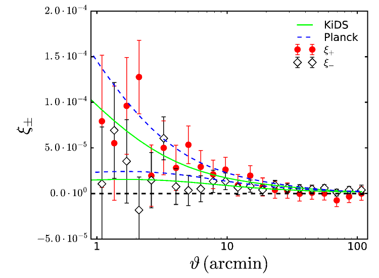
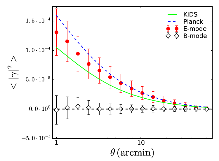
Based on the above analyses, we computed the shear 2PCFs using the combined VOICE shear catalogue from the four CDFS tiles. The results are shown in Fig. 9. The upper left panel shows $\xi_{+}$ (red full dots) and $\xi_{-}$ (black open diamonds), respectively. The upper limit of the angular separation considered here is taken to be $120\arcmin$, as the survey area is $2\times 2\hbox{ deg}^{2}$. For the lower limit, although we show the results from $\vartheta=1\arcmin$ in Fig. 9, we actually calculate $\xi_{\pm}$ starting from $10\arcsec$, which corresponds to the LensFit postage stamp size (48 pixels).

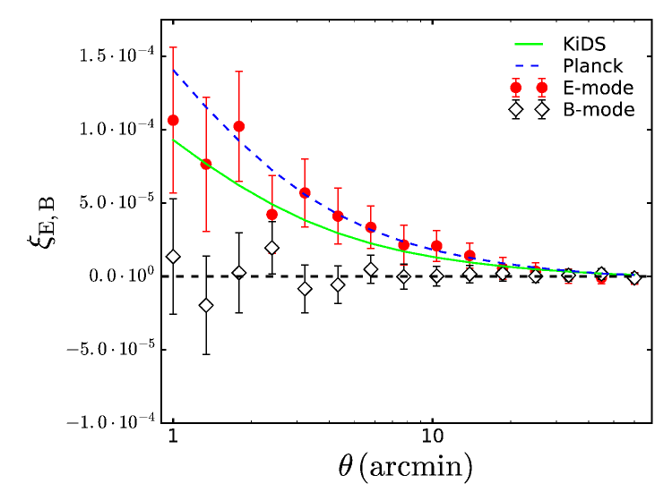
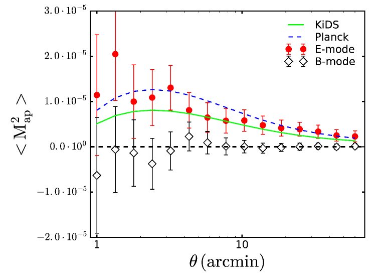
The other three panels in Fig. 9 show the results of $\xi_{\rm E,B}$ (top-right), $\langle M_{{\rm ap}}^{2}\rangle$ (bottom-left) and $\langle|\gamma|^{2}\rangle$ (bottom-right), respectively. They are derived from $\xi_{\pm}$ by performing integrations with different filters. To avoid introducing artificial B-mode due to the finite integration range, we considered these three quantities only up to the angular scale $\theta=60\arcmin$, the radius of an aperture with maximum separation in a galaxy pair. It is seen that the B-mode is consistent with zero for all the three derived quantities in the given angular range. The multiplicative biases of $\xi_{\pm}$ have been corrected (Eq. 12 and 13). The amplitudes of the corrections on 2PCFs are in the order of a few percent.

The different filter functions of three derived second-order functions lead to different sensitivities on smoothing scales. For instance, $\langle|\gamma|^{2}\rangle$ is the one with the highest correlation between data points, thus the E-/B-mode components look smoother than those of the other two quantities. The error bars are the squared root of the diagonal terms of the covariance matrix measured from VOICE-like ray-tracing simulations to be described in Sect. 4.4.

The results are compared to the theoretical predictions using the cosmological parameters derived from KiDS (Hildebrandt et al., 2017) and Planck15 (Planck Collaboration et al., 2016), where $\Omega_{\rm m}=0.231;\sigma_{8}=0.851$ and $\Omega_{\rm m}=0.315;\sigma_{8}=0.831$ respectively, with the same angular scale range $[10\arcsec,120\arcmin]$ for $\xi_{\pm}$. The redshift distribution used for the theoretical predictions is obtained by fitting the Eq. (1) to the photo-$z$ distribution of the VOICE shear catalogue, and is shown as a solid line in Fig. 7.

4.4 Covariance Estimation

To model and interpret the observed 2PCFs, we need to estimate the error covariance. To do so, we used the N-body simulations described in Liu et al. (2015) to account for the non-Gaussianity of the cosmic shear field on small and medium angular scales, and performed ray-tracing calculations to construct the shear and convergence maps. The cosmology involved is the flat $\Lambda$ cold dark matter ($\Lambda$CDM) model with $\Omega_{\mathrm{m}}=0.28$, $\Omega_{\Lambda}=0.72$, $\Omega_{\mathrm{b}}=0.046$, $\sigma_{8}=0.82$, $n_{s}=0.96$ and $h=0.7$, where $\Omega_{\rm m}$, $\Omega_{\Lambda}$, and $\Omega_{\rm b}$ are the present dimensionless densities of the total matter, cosmological constant, and the baryonic matter, respectively, $\sigma_{8}$ is the rms of linearly extrapolated density perturbations over $8\hbox{ Mpc}h^{-1}$, $n_{s}$ is the power index of the power spectrum of initial density fluctuations, and $h$ is the Hubble constant in units of $100\hbox{ km/s/Mpc}$. In order to cover a large redshift range up to $z=3$ in ray-tracing calculations, we padded 12 independent simulation boxes, with 8 small boxes each with a size of $320\hbox{ Mpc}h^{-1}$ to $z=1$ and 4 larger boxes each with a size of $600\hbox{ Mpc}h^{-1}$ from $z=1$ to $z=3$, and used in total 59 lens planes. From one set of padded boxes, we can generate 4 sets of lensing maps each with an area of $3.5\times 3.5\deg^{2}$ sampled on $1024\times 1024$ pixels. For each set, we have 59 shear and 59 convergence maps at 59 different redshifts corresponding to the far edges of the 59 lens planes. In total, we run 24 sets of simulations, and generate lensing maps with the total area of $1176\deg^{2}$. A more detailed descriptions for our N-body simulations and ray-tracing calculations can be found in Liu et al. (2015) and Liu et al. (2014).

With these lensing maps, we then generated 384 VOICE-like mock catalogues to estimate the error covariance. The generating procedure for each mock is as follows.

(i) We placed the 4 continuous VOICE tiles randomly over the simulated map area, with the positions, photo-$z$, galaxy weights and the mask information preserved in the analyses. The amplitudes of ellipticities of the galaxies were also preserved, but with their orientations being randomized.

(ii) For each galaxy in the catalogue, its reduced shear $\bm{g}$ was calculated by interpolating the signals from the pixel positions on simulated maps to the galaxy position. The interpolation was also done in redshift. Regarding the randomized ellipticity obtained in (i) as its intrinsic ellipticity $\bm{\epsilon_{s}}$, the mock observed ellipticity $\bm{\epsilon}$ can then be constructed from

$$\bm{\epsilon}(\bm{\vartheta},z)=\left\{\begin{array}[]{ll}\frac{\bm{\epsilon}_{s}(\bm{\vartheta},z)+\bm{g}(\bm{\vartheta},z)}{1+\bm{g^{*}}(\bm{\vartheta},z)\bm{\epsilon}_{s}(\bm{\vartheta},z)}&\textrm{for $|{\bm{g}(\bm{\vartheta},z)}|\leq 1$}\\ \\ \frac{1+\bm{g}(\bm{\vartheta},z)\bm{\epsilon}_{s}^{*}(\bm{\vartheta},z)}{\bm{\epsilon}_{s}^{*}(\bm{\vartheta},z)+\bm{g^{*}}(\bm{\vartheta},z)}&\textrm{for $|{\bm{g}(\bm{\vartheta},z)}|>1$}\end{array}\right..$$ (14)

(iii) The 2PCFs analyses were then carried out for each mock, with the same procedures for the observed data, the error covariance can be further estimated with these 2PCFs results from the whole 384 mocks. These covariance matrices were used to give error bars shown in Fig.9, and also applied to derive cosmological constraints to be presented in Sect. 5.

4.5 The star-galaxy cross-correlation function

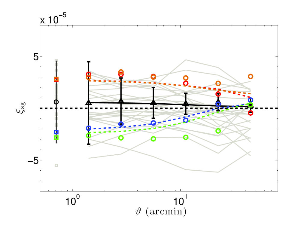
The results in Fig. 9 show that our VOICE shear catalogue exhibits no detectable B-mode. To further check the data quality, we analyze the level of PSF-related systematics by measuring the star-galaxy cross correlation $\bm{\xi}_{\rm sg}(\vartheta)=\langle\epsilon^{\rm obs}\bm{e^{\star}}\rangle$, where $\epsilon^{\rm{obs}}$ is the observed shear estimators, $\bm{e^{\star}}$ is a complex $N$ dimensional vector of PSF ellipticity at the position of the galaxy in each of the $N$ dithered exposures of the field. For these analyses, star-galaxy pairs with the angular separation $\vartheta$ in the range of $[1\arcmin,60\arcmin]$ were taken into account, and they were divided into 6 evenly-distributed log-normal bins. The zero-lag star-galaxy correlation $\bm{\xi}_{\rm sg}(\vartheta=0)$, hereafter $\bm{\xi}_{\rm sg}(0)$, which indicates the primary systematics, was derived using the model of PSF ellipticity to determine $\bm{e^{\star}}$ at the location of each galaxy, with

$$\bm{\xi}_{\rm sg}(0)=\frac{\Sigma{w_{i}[\epsilon_{1}(\bm{\vartheta_{i}})\bm{e_{1}^{\star}}(\bm{\vartheta_{i}})+\epsilon_{2}(\bm{\vartheta_{i}})\bm{e_{2}^{\star}}(\bm{\vartheta_{i}})]}}{\Sigma{w_{i}}}.$$ (15)

If the PSF model and correction are correct so that the observed shear estimator is uncorrelated with the PSF, $\bm{\xi}_{\rm sg}(0)$ should be consistent with zero.

Following some arguments discussed in Heymans et al. (2012b), with a measure of the zero-lag star-galaxy correlation $\bm{\xi}_{\rm sg}(0)$, we can make a prediction of the star-galaxy correlation at any angular scale using

$$\bm{\xi}_{\rm sg}(\vartheta)\approx\bm{C}_{0}^{-1}\bm{\xi}_{\rm sg}(0)\bm{C}_{\vartheta},$$ (16)

where $\bm{C}_{0}$ is the measured covariance matrix of PSF ellipticities between exposures at zero-lag and $\bm{C}_{\vartheta}$ is the same PSF measurement but for sources at separation $\vartheta$. Here we only consider the case using weighted PSF ellipticities in the final shear catalogues. Thus, Eq. (16) reduces to

$$\xi_{\rm sg}(\vartheta)\approx\xi_{\rm sg}(0)\langle e_{a}^{\star}e_{b}^{\star}\rangle/\langle e^{\star 2}\rangle,$$ (17)

where $a$ and $b$ indicate objects separated by a distance $\vartheta$.

Fig. 10 shows the star-galaxy cross-correlation function $\xi_{\rm sg}(\vartheta)$ measured in CDFS1-4 fields. Generally speaking, the whole star-galaxy cross-correlation function is consistent with zero and is well within the range of values observed in the KiDS survey.

Figure 10: The star-galaxy cross-correlation function $\xi_{\rm sg}(\vartheta)$ measured in CDFS1-4 (e.g., black triangles with error bars), compared to the predicted angular star-galaxy correlation (e.g., Eq. 17, black solid line) calculated using only the zero separation measure $\xi_{\rm sg}(0)$ (shown offset, gray circle with error bar). The corresponding error bars are assigned using the standard deviation of $\xi_{+}$ at the corresponding $\vartheta$ evaluated from the constructed 384 mocks. Blue, red, green and orange circles without error bars are the measured star–galaxy cross-correlation function for CDFS1, CDFS2, CDFS3 and CDFS4, respectively. The corresponding squares and dash lines are the corresponding zero-lag and predicted measures for different individual fields. As a comparison, the bright grey lines are the measured star-galaxy cross-correlation function for the 24 G15 fields in the KiDS survey.

4.6 Tomography check

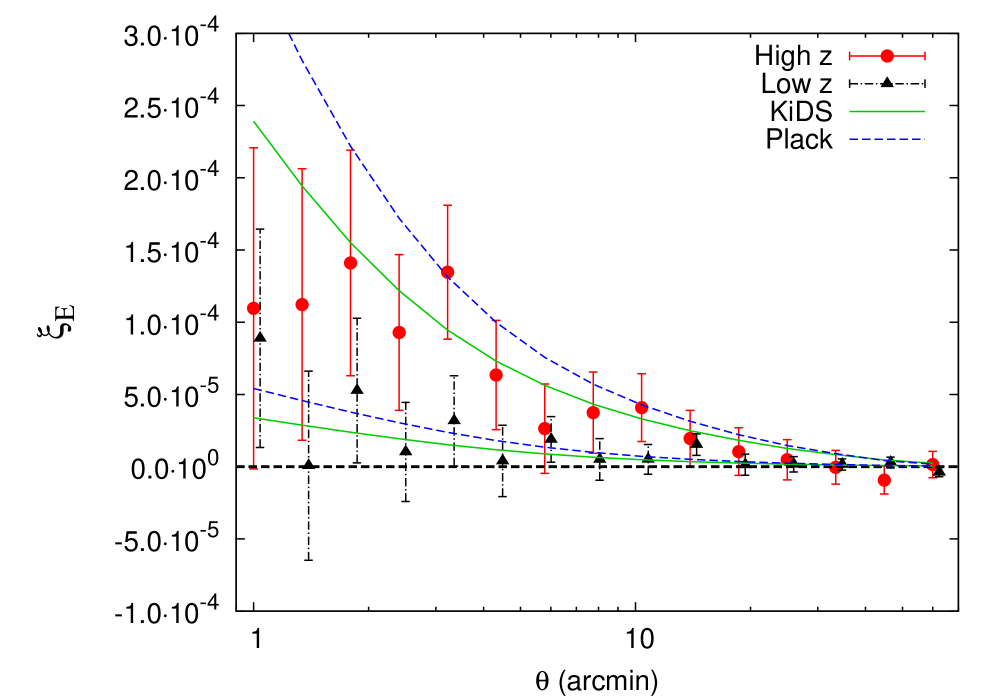
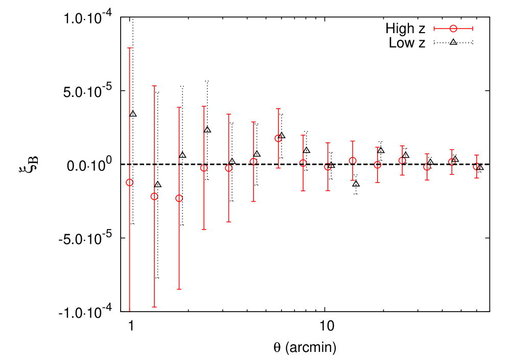
The reliability of shear measurement in the VOICE data can be further tested by considering the tomographic shear signals. We separate the full shear sample into two photo-$z$ bins divided by the median photo-$z$ of 0.83. The results of $\xi_{\rm E}$ (left) and $\xi_{\rm B}$ (right) are shown in Fig. 11. As expected, the shear correlation of the high redshift bin is higher than that of the low redshift bin. There are no obvious B-modes in all angular scales in both of cases. The solid green lines are the theoretical predictions assuming the KiDS and Planck15 cosmology with the redshift distributions for the two bins directly from the photo-$z$ measurements. We can see that our results are in good agreements with the theoretical predictions.

As this paper mainly focuses on the shear measurement of VOICE, the tomographic results presented here are only for checking the reliability of the shape measurement. Being our next task, we will perform cosmological studies using the tomographic correlations from VOICE. For that, we will consider carefully the impacts of galaxy intrinsic alignments and photo-$z$ errors.

Figure 11: The calibrated shear correlation functions $\xi_{\rm E}$ (left panel) and $\xi_{\rm B}$ (right panel) of two photo$-z$ bin samples. The calculation of error bars and the theoretical predictions are the same as those of Fig. 9. The theoretical predictions are estimated using the cosmological parameters derived from KiDS (green solid lines) and Planck15 (blue dash lines).

4.7 Blending Effect

The final mosaic reaches a $5\sigma$ limiting magnitude of $r_{\mathrm{AB}}$ $\sim$ 26.1 mag with $2\arcsec$ aperture diameter for point sources. Over 488,000 galaxies are detected with a number density of 32.85 arcmin^-2 after excluding the masked regions. Following Chang et al. (2013), we define the neighbors simply by their separation on the celestial sphere. We find that only 0.04% of galaxies have neighbors within $1.0\arcsec$, while the fraction increases dramatically to over 16% within a 3.0$\arcsec$ separation. These galaxies can be either physically related neighbors which have similar shear or projected close pairs, with different redshifts and shape distortions. Though LensFit has encoded an algorithm to deal with them (Miller et al., 2013), potential bias is still inevitable in the measured shear due to the inappropriate modeling of the surface brightness distributions in the overlapping regions.

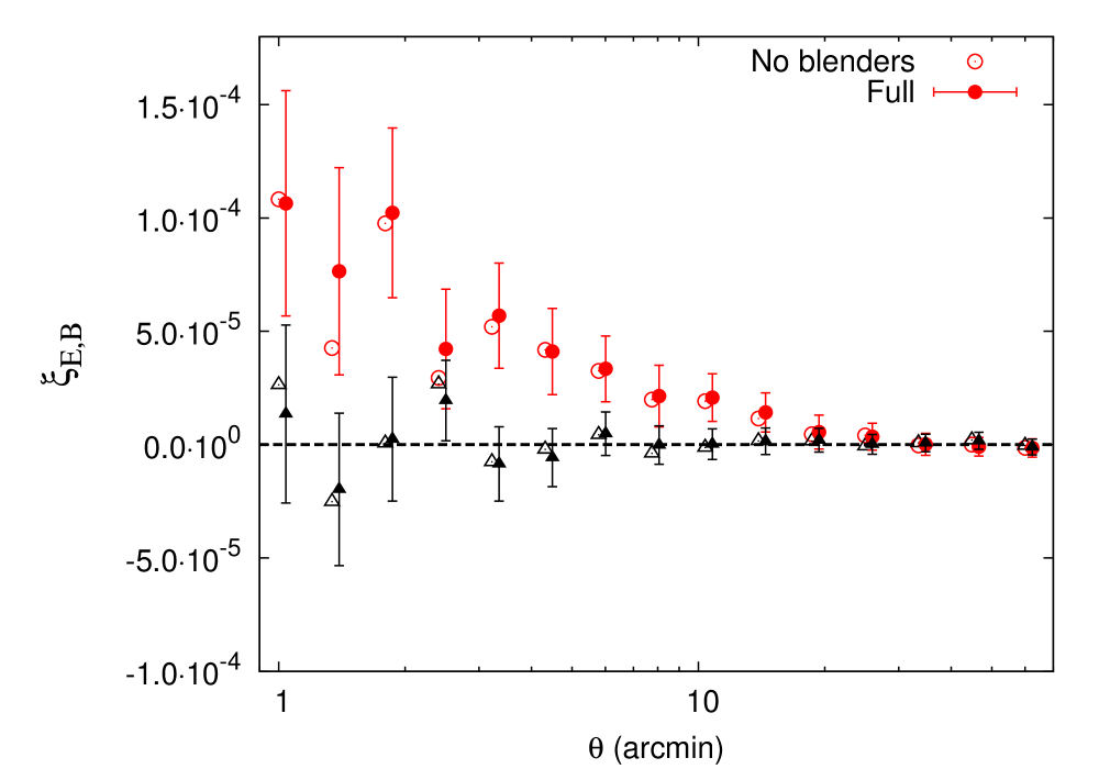
Although most of the neighbors have been excluded by LensFit, about 31.6% of the neighboring galaxies within separation $r=3.0\arcsec$ still have shape measurements. The ellipticity dispersion of these remainders is 3.4% larger than the overall dispersion. Their weighted number density is about 1.28 arcmin^-2. We compare the shear two-point correlation functions of the full sample and that derived after rejecting neighbors within $r\leq 3.0\arcsec$. The results are shown in Fig. 12. We find that the differences are within the error bars given the relatively large statistical uncertainties of the VOICE shear sample. For future large surveys with dramatically reduced statistical errors, the neighboring contaminations need to be carefully accounted for.

From our image simulations (Liu et al., 2018), we further quantify the impact of the close neighbors on the multiplicative biases. It is found that the SNR of these galaxies are systematically overestimated by LensFit due to the contamination of the neighboring galaxy. As a result, these close neighbors do provide an additional contribute to the multiplicative bias, especially at high SNR. The weighted average bias resulting from these neighbors is about 0.002 from our simulation analyses. Although this can be safely neglected for the VOICE analyses, it can be a serious concern for future large surveys that need the multiplicative bias to be controlled at the level less than 0.001.

Figure 12: The calibrated shear correlation function $\xi_{\rm{E,B}}$ after excluding the blended galaxies (open symbol) is compared to that of the full galaxy sample (solid symbol). The E-modes are circle in red and the B-modes are triangle in black. The uncertainties are calculated as in Fig. 9.

5 Cosmological Constraints

The most sensitive constraints from weak lensing alone are the cosmological parameters of the matter density $\Omega_{\rm m}$ and the linear amplitude of mass fluctuations $\sigma_{8}$. In this section, we present the marginalized constraints for $\Omega_{\rm m}$ and $\sigma_{8}$ in a flat $\Lambda$CDM cosmological model. We note that the main focus of the paper is to present the shear measurements. The cosmological constraints shown here are presented as a reliability check, in addition to the 2PCFs presented in the previous sections. Considering also the relatively large statistical uncertainties of the VOICE shear catalog, here we do not discuss different possible systematics, such as galaxy intrinsic alignments, baryonic effects, photo-$z$ errors, etc.. We will do more careful cosmological analyses as our next task.

5.1 Sampling the posterior

We use the open source code Cosmo_PMC (Kilbinger et al., 2011) to sample the VOICE weak-lensing constraint posterior with Population Monte Carlo (PMC). For the flat $\Lambda$CDM model, the base parameters are $\Omega_{\rm m}$, $\sigma_{8}$, $\Omega_{\rm b}$, $n_{\rm s}$ and $h$. The prior ranges are summarized in Table 3.

The perplexity parameter $p$ of Cosmo_PMC is a value between 0 and 1, where 1 stay for a perfect agreement between importance function and the posterior. Generally, $p$ reaches 0.7 after 10 iterations, after which we stopped the iterations. We used 30,000 sample points in each iteration. For the last iteration, larger samples with 300,000 points are used to reduce the Monte-Carlo variance.

Table 3: The parameters sampled under the weak-lensing posterior. The second column indicates the (flat) prior ranges analyzed with flat $\Lambda$CDM.

Param.	Prior	Description
$\Omega_{\rm m}$	$[0;1.2]$	Total matter density
$\sigma_{8}$	$[0.2;1.5]$	Power-spectrum normalisation
$\Omega_{\rm b}$	$[0;0.1]$	Baryon density
$n_{\rm s}$	$[0.7;1.2]$	Spectral index of prim. density fluct.
$h$	$[0.4;1.2]$	Hubble parameter

5.2 Choice of second-order estimators

We mainly use the aperture mass dispersion $\langle M_{\rm ap}^{2}\rangle$ for deriving cosmological constraints, for the following reasons. 1) The filter function of $\langle M_{\rm ap}^{2}\rangle$ is much narrower compared to the one of top-hat shear rms $\langle|\gamma|^{2}\rangle$. Thus $\langle M_{\rm ap}^{2}\rangle$ of different smoothing scales $\theta$ are less correlated. 2) For $\langle M_{\rm ap}^{2}\rangle$, only the lower angular limit is problematic and causes leakage of the B-mode into the E-mode signal on small smoothing scales.

Anderson (2003) and Hartlap et al. (2007) have shown that the inverse covariance calculated directly from the covariance matrix constructed from simulations is biased, resulting in a biased maximum likelihood (ML) estimator. We correct the ML estimator by multiplying per the Anderson-Hartlap factor $A=(n-p-2)/(n-1)$ (Hartlap et al., 2007). The bias depends on the number of simulations $n$ and the number of data bins $p$. Here we have $n=384$ and $p=15$. Thus the correct factor is $A=0.96$.

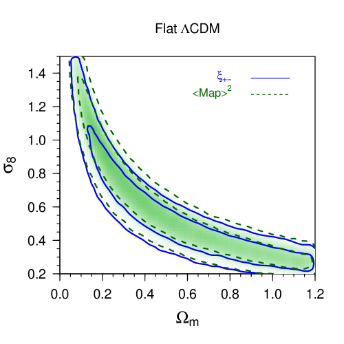
Before presenting the main constraints, we first check the consistency by comparing the constraints from $\langle M_{\rm ap}^{2}\rangle$ and those from the 2PCFs $\xi_{\pm}$ for the flat $\Lambda$CDM model. The results are shown in Fig. 13. It is seen that the two second-order quantities give rise to very similar contours in the plane of $\Omega_{\rm m}$ and $\sigma_{8}$. This demonstrates that the B-mode of $\langle M_{\rm ap}^{2}\rangle$ has negligible impact on the cosmological parameters constraints.

5.3 Results

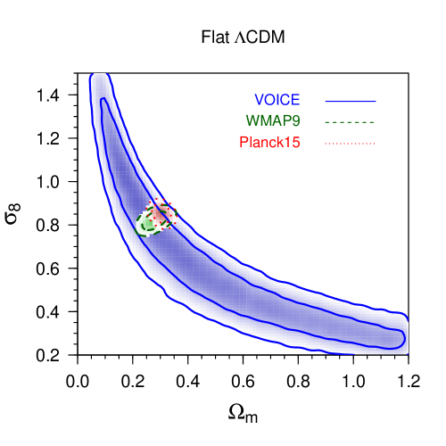
The goal of this paper is to present the VOICE shear catalog measurements, which we have used to obtain the marginalized constraints of $\Omega_{\rm m}$ and $\sigma_{8}$ for flat $\Lambda$CDM cosmological model in Fig. 14. The degeneracy direction of these two parameters is approximately a power law, while its amplitude is given by the parameter $\Sigma_{8}=\sigma_{8}(\Omega_{\rm m}/0.3)^{\alpha}$.

In order to compare to the results from the KiDS analyses, we fix $\Omega_{\rm m}=0.3$ and derive the constraints of $\Sigma_{8}$ and $\alpha$. We obtain $\Sigma_{8}=0.70^{+0.11}_{-0.12}$ and $\alpha=0.64\pm 0.02$ assuming a $\Lambda$CDM model, while by fixing $\alpha=0.5$, as done for KiDS-450 (Hildebrandt et al., 2017), we obtain $\Sigma_{8}=0.68^{+0.11}_{-0.15}$. These results are in broad agreements with the ones from KiDS-450 and from other literature, showing that our shear measurements are not affected by systematics comparing to the statistical uncertainties.

Finally, we compare these results with constraints derived from CMB measurements from WMAP9 (green) and Planck15 (TT + lowP, red) in Fig. 14. The VOICE constraints are in broad agreements with both, due to the relatively large statistical uncertainties. However, we note that, despite being statistically consistent, a mild offset with PLANCK15 can still be seen, which goes in the same direction of the tension found by KiDS-450. A similar tension is seen if we compare with Planck polarization data (TT $+$ TE $+$ EE $+$ lowP), again despite the large statistic error of VOICE shear 2PCF.

To conclude, the above analyses mainly show the validity of our shear catalog and the consistency with other results based on wider but shallower datasets. The detailed cosmological studies taking into account different systematics will be presented in a forthcoming paper.

Figure 13: Marginalized posterior density contours (68.3 per cent and 95.5 per cent) for $\Omega_{\rm m}$ and $\sigma_{8}$ are constrained from $\xi_{\pm}$ and $\langle M_{\rm ap}^{2}\rangle$ in the case of flat $\Lambda$CDM.

Figure 14: Marginalized posterior density contours (68.3 per cent, 95.5 per cent) of $\Omega_{\rm m}$ and $\sigma_{8}$ for flat $\Lambda$CDM from VOICE weak lensing (blue), WMAP9 (green) and Planck15 (red).

6 Summary

We have presented the cosmic shear measurement of the 4.9 deg² CDFS field from $r$-band images of the VOICE survey at the VST/OmegaCAM. Each of the four pointings covering the area has been observed with more than 100 exposures. After a stringent selection for high quality data, including cuts on seeing and sky background brightness variation, about one-third of the exposures have been used to obtain the shear measurement. The final $r$-band co-added image reaches a $r=26.1$ $5\sigma$ limiting magnitude for point sources, which is 1.2 mag deeper than KiDS. We have used the software LensFit to measure the galaxy shapes, which was successfully applied on CFHTLenS and KiDS. The novelty of our approach, though, is that this is the first time that LensFit is applied to a deep survey with more than a few tens exposures. To check the accuracy of our shear measurement we have used VOICE-like imaging simulations, which have been fully illustrated in a companion paper (Liu et al., 2018). From the mock observations, we have obtained the multiplicative bias calibration values at different galaxy SNR and size bins to correct the real measurements. After these calibrations, the final residual multiplicative bias of LensFit shear measurement is measured with an accuracy of 0.03 with negligible addictive bias. The final VOICE-CDFS shear catalogue contains more than $3\times 10^{5}$ galaxies with non-zero weight, corresponding to the effective number density of galaxies of 16.35 arcmin^-2, about twice the one of KiDS. The photo-$z$ of each galaxy have been estimated using the VOICE $u,g,r,i$ together with the near-infrared $Y,J,H,K_{s}$ VIDEO data. The mean redshift of the shear catalogue is 0.87, considering shear weights.

To check the reliability of the VOICE shear catalogue, we have calculated the star-galaxy cross-correlations. Generally speaking, the whole star-galaxy cross-correlation function has been found consistent with zero. We further calculated the 2D shear 2PCFs and the derived second-order statistics, and those with two tomographic redshift bins divided by the median redshift 0.83 of the sample. The results are in agreement with the theoretical predictions using the cosmological parameters derived from KiDS and Planck15.

VOICE is a deep imaging survey, and it is important to assess the impact of possible blending effect. As discussed in detail in Liu et al. (2018), although most of the neighbours have been excluded by LensFit, about 31.6% of the neighbouring galaxies within separation $r=3.0\arcsec$ still have shape measurements. By comparing the shear two-point correlation functions between the full sample and that after rejecting $r\leq 3.0\arcsec$ neighbors, we have found that the impact of these neighbouring galaxies on the shear correlations is within the VOICE statistical uncertainties. This can be a serious concern, however, for future large and deep surveys.

To further validate our shear measurements, we have derived cosmological constraints from the second-order shear statistics $\langle M_{\rm ap}^{2}\rangle$. We have shown the marginalized constraints for $\Omega_{\rm m}$ and $\sigma_{8}$ of flat $\Lambda$CDM cosmological model, which has found to be $\Sigma_{8}=\sigma_{8}(\Omega_{\rm m}/0.3)^{0.5}=0.68^{+0.11}_{-0.15}$. This result is fully consistent with other literature weak lensing studies which demonstrated that, despite the larger uncertainties, our approach was able to keep all systematics under control.

Having tested the quality of our shear catalogue, the next step will be to carry out detailed cosmological studies with different systematics carefully accounted for. Furthermore, our results will allow us to detect galaxy clusters over a broad redshift range, and constrain their mass distribution from VOICE shear catalogue.

Appendix A Photometric redshift using only optical bands

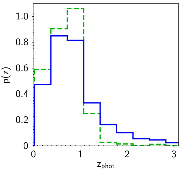
In order to show the improvement of photo-$z$ measurements by adding near-infrared data, we estimate the photo-$z$ using VOICE optical bands data (4-band photo-$z$) only. We then match the 4-band photo-$z$ catalog with the 8-band photo-$z$ for non-zero LensFit weight galaxies. The redshift distribution histograms for the matched galaxies are shown in Fig. 15. A significant difference is seen at $z>1$ between the two photo-$z$ estimates. Without the near-infrared data, $\sim$15% of galaxies with 8-band $z>1$ are assigned to lower redshifts.

As in Sect. 3.4, we also compare the 4-band photo-$z$ with the spec-$z$. The median value of $\delta z=($photo-$z-$spec-$z)/(1+$spec-$z)$ and MAD values are $-0.010$ and $0.073$, respectively, which are $\sim$20% larger than those of 8-band photo-$z$ (see Table 4). We further separate galaxies into low-$z$ (4-band photo-$z<$ 0.83) and high-$z$ (4-band photo-$z\geq$ 0.83) bins, and list median $\delta z$ and MAD values in Table 4. In comparison with the results of 8-band photo-$z$, about one-third of 8-band high-$z$ galaxies are shifted to the 4-band low-$z$ bin. The offset $\delta z$ in high-$z$ bin is $\sim$3 times larger than that of 8-band photo-$z$.

Figure 15: The normalized histogram of photo-$z$ estimated using optical bands (4-band photo-$z$, green dash line), optical and near-infared bands (8-band photo-$z$, blue solid line) are shown, without considering the shear weight.

Table 4: The number of spec-$z$ matched galaxies, their median $\delta z$ and MAD values are listed for all $z$, low-$z$ and high-$z$ bins.

			Ngal	$\delta z$	MAD
8-band photo-$z$		all	23638	$-0.008$	0.060
		low-$z$	19389	$-0.012$	0.055
		high-$z$	4069	0.022	0.104
4-band photo-$z$		all	23638	$-0.010$	0.073
		low-$z$	20168	$-0.015$	0.067
		high-$z$	3300	$0.063$	0.160

Fig. 16 shows the cosmological constraints of $\sigma_{8}$ and $\Omega_{\rm m}$ under the $\Lambda$CDM model using the 4-band photo-$z$. Compared to the constraints using 8-band photo-$z$, the contours are shifted to the higher $\sigma_{8}$ and $\Omega_{\rm m}$ side. The $\Sigma_{8}=\sigma_{8}(\Omega_{\rm m}/0.3)^{0.5}$ is shifted from $0.68^{+0.11}_{-0.15}$ to $0.74^{+0.13}_{-0.16}$. Such a shift is in line with the fact that 15% of the high-$z$ galaxies in the 8-band photo-$z$ catalog are assigned to low-$z$ bin.

Figure 16: Marginalized posterior density contours (68.3 per cent and 95.5 per cent) for $\Omega_{\rm m}$ and $\sigma_{8}$ are constrained from $\langle M_{\rm ap}^{2}\rangle$ in the case of flat $\Lambda$CDM. The blue contours are the constraints using 8-band photo-$z$, while the green are the results using 4-band photo-$z$.

References

- Aihara et al. (2018) Aihara H., et al., 2018, PASJ, 70, S4
- Anderson (2003) Anderson T. W., 2003, An introduction to multivariate statistical analysis, 3rd edn.. Wiley-Interscience
- Barbary (2016) Barbary K., 2016, The Journal of Open Source Software, 1
- Bartelmann & Schneider (2001) Bartelmann M., Schneider P., 2001, Phys. Rep., 340, 291
- Becker et al. (2016) Becker M. R., et al., 2016, Phys. Rev. D, 94, 022002
- Benítez (2011) Benítez N., 2011, BPZ: Bayesian Photometric Redshift Code, Astrophysics Source Code Library (ascl:1108.011)
- Benítez et al. (2004) Benítez N., et al., 2004, ApJS, 150, 1
- Benjamin et al. (2013) Benjamin J., et al., 2013, MNRAS, 431, 1547
- Bertin (2011) Bertin E., 2011, in Evans I. N., Accomazzi A., Mink D. J., Rots A. H., eds, Astronomical Society of the Pacific Conference Series Vol. 442, Astronomical Data Analysis Software and Systems XX. p. 435
- Bertin & Arnouts (1996) Bertin E., Arnouts S., 1996, A&AS, 117, 393
- Botticella et al. (2017) Botticella M. T., et al., 2017, A&A, 598, A50
- Capaccioli & Schipani (2011) Capaccioli, M., & Schipani, P. 2011, The Messenger, 146, 2
- Cappellaro et al. (2015) Cappellaro E., et al., 2015, A&A, 584, A62
- Chang et al. (2013) Chang C., et al., 2013, MNRAS, 434, 2121
- Coleman et al. (1980) Coleman G. D., Wu C.-C., Weedman D. W., 1980, ApJS, 43, 393
- Crittenden et al. (2002) Crittenden R. G., Natarajan P., Pen U.-L., Theuns T., 2002, ApJ, 568, 20
- de Jong et al. (2015) de Jong J. T. A., et al., 2015, A&A, 582, A62
- de Jong et al. (2017) de Jong J. T. A., et al., 2017, A&A, 604, A134
- De Cicco et al. (2015) De Cicco D., et al., 2015, A&A, 574, A112
- Falocco et al. (2015) Falocco S., et al., 2015, A&A, 579, A115
- Fu & Fan (2014) Fu L.-P., Fan Z.-H., 2014, Research in Astronomy and Astrophysics, 14, 1061
- Fu et al. (2014) Fu L., et al., 2014, MNRAS, 441, 2725
- Gaia Collaboration et al. (2016) Gaia Collaboration et al., 2016, A&A, 595, A2
- Grado et al. (2012) Grado A., Capaccioli M., Limatola L., Getman F., 2012, Memorie della Societa Astronomica Italiana Supplementi, 19, 362
- Hartlap et al. (2007) Hartlap J., Simon P., Schneider P., 2007, A&A, 464, 399
- Heymans et al. (2012a) Heymans C., et al., 2012a, MNRAS, 427, 146
- Heymans et al. (2012b) Heymans C., et al., 2012b, MNRAS, 427, 146
- Hildebrandt et al. (2017) Hildebrandt H., et al., 2017, MNRAS, 465, 1454
- Hinshaw et al. (2013) Hinshaw G., et al., 2013, ApJS, 208, 19
- Huang et al. (2011) Huang Z., Radovich M., Grado A., Puddu E., Romano A., Limatola L., Fu L., 2011, A&A, 529, A93
- Jarvis et al. (2013) Jarvis M. J., et al., 2013, MNRAS, 428, 1281
- Jarvis et al. (2016) Jarvis M., et al., 2016, MNRAS, 460, 2245
- Jee et al. (2013) Jee M. J., Tyson J. A., Schneider M. D., Wittman D., Schmidt S., Hilbert S., 2013, ApJ, 765, 74
- Jee et al. (2016) Jee M. J., Tyson J. A., Hilbert S., Schneider M. D., Schmidt S., Wittman D., 2016, ApJ, 824, 77
- Kaiser (1992) Kaiser N., 1992, ApJ, 388, 272
- Kilbinger (2015) Kilbinger M., 2015, Reports on Progress in Physics, 78, 086901
- Kilbinger et al. (2011) Kilbinger M., et al., 2011, preprint, (arXiv:1101.0950)
- Kilbinger et al. (2013) Kilbinger M., et al., 2013, MNRAS, 430, 2200
- Kinney et al. (1996) Kinney A. L., Calzetti D., Bohlin R. C., McQuade K., Storchi-Bergmann T., Schmitt H. R., 1996, ApJ, 467, 38
- Kitching et al. (2008) Kitching T. D., Miller L., Heymans C. E., van Waerbeke L., Heavens A. F., 2008, MNRAS, 390, 149
- Kuijken et al. (2015) Kuijken K., et al., 2015, MNRAS, 454, 3500
- Liu et al. (2014) Liu X., Wang Q., Pan C., Fan Z., 2014, ApJ, 784, 31
- Liu et al. (2015) Liu X., et al., 2015, MNRAS, 450, 2888
- Liu et al. (2016) Liu X., et al., 2016, Physical Review Letters, 117, 051101
- Liu et al. (2018) Liu D., et al., 2018, MNRAS, in press
- Mandelbaum (2017) Mandelbaum R., 2017, preprint, (arXiv:1710.03235)
- Mandelbaum et al. (2018) Mandelbaum R., et al., 2018, PASJ, 70, S25
- Miller et al. (2007) Miller L., Kitching T. D., Heymans C., Heavens A. F., van Waerbeke L., 2007, MNRAS, 382, 315
- Miller et al. (2013) Miller L., et al., 2013, MNRAS, 429, 2858
- Planck Collaboration et al. (2016) Planck Collaboration et al., 2016, A&A, 594, A13
- Rowe et al. (2015) Rowe B. T. P., et al., 2015, Astronomy and Computing, 10, 121
- Schneider et al. (2002a) Schneider P., Van Waerbeke L., Mellier Y., 2002a, A&A, 389, 729
- Schneider et al. (2002b) Schneider P., van Waerbeke L., Kilbinger M., Mellier Y., 2002b, A&A, 396, 1
- Schrabback et al. (2010) Schrabback T., et al., 2010, A&A, 516, A63
- Semboloni et al. (2006) Semboloni E., et al., 2006, A&A, 452, 51
- Skrutskie et al. (2006) Skrutskie M. F., et al., 2006, AJ, 131, 1163
- Vaccari (2015) Vaccari M., 2015, Proceedings of ”The many facets of extragalactic radio surveys: towards new scientific challenges” Conference, 20-23 October 2015, Bologna, Italy, Proceedings of Science, 267, 27
- Vaccari et al. (2010) Vaccari M., et al., 2010, A&A, 518, L20
- Vaccari et al. (2016) Vaccari M., et al., 2016, Proceedings of the 4th Annual Conference on High Energy Astrophysics in Southern Africa, 25-26 August 2016, Cape Town, South Africa, Proceedings of Science, 275, 26