Nonlinear dynamics of a semiquantum Hamiltonian in the vicinity of quantum unstable regimes

Abstract

We examine the emergence of chaos in a non-linear model derived from a semiquantum Hamiltonian describing the coupling between a classical field and a quantum system. The latter corresponds to a bosonic version of a BCS-like Hamiltonian, and possesses stable and unstable regimes. The dynamics of the whole system is shown to be strongly influenced by the quantum subsystem. In particular, chaos is seen to arise in the vicinity of a quantum critical case, which separates the stable and unstable regimes of the bosonic system.

I Introduction

The interplay between quantum and classical systems is a topic of great interest in quantum dynamics and quantum chaos. Whenever quantum effects in one of the systems are negligible in comparison with those of the other, its consideration as classical simplifies the description and provides deep insight into the combined system dynamics. Examples can be readily found, such as Bloch equations Bloch , two-level systems interacting with an electromagnetic field within a cavity and Jaynes-Cummings semi-classical model Milonni ; Sa.91 , collective nuclear motion Ring , etc. Here we will consider a semiquantum bipartite system in which the quantum component, representing the matter and described by a quadratic Hamiltonian in boson operators or generalized coordinates and momenta, can exhibit distinct dynamical regimes RK.05 ; RK.09 (bounded or unbounded), whereas the classical component represents a single mode of an electromagnetic field. Such type of composite system is of interest in Quantum Optics and Condensed Matter Milonni ; Sa.91 ; K0 ; K1 . The essential point we want to discuss is how the different regimes of the quantum system influence those of the combined semiquantum system, and in particular examine if the onset of chaos can be related to this effect.

As is well known, quadratic Hamiltonians in generalized coordinates and momenta, or equivalently in boson operators, are a common presence in theoretical models of physical systems. They often emerge through diverse linearization procedures of the pertinent equations of motion around a stationary point Ring ; BR.86 , providing a tractable description of the small amplitude fluctuations which is exact if the deviations from equilibrium are sufficiently small. They play in particular a fundamental role in the description of Bose-Einstein condensates (BEC) GM.97 ; PB.97 ; AK.02 ; F.07 ; E.07 ; F.08 as well as in other fields like disordered systems GC.02 , quantum optics Sa.91 , dynamical systems P.97 ; Do.00 ; Ko.00 and collective nuclear motion Ring . While the treatment of such quadratic systems in the stable regime is of course standard, leading to a set of normal coordinates which evolve independently, that of the unstable regime, in which the quadratic Hamiltonian is no longer positive definite, is less trivial and requires the introduction of non-hermitian normal coordinates (complex normal modes) RK.05 ; RK.09 ; RRC.14 , which exhibit exponential evolutions. Moreover, at the boundary between stable and unstable sectors, non-separable regimes can arise in which the dynamics is described by non-diagonalizable evolution matrices and the equations of motion cannot be fully decoupled RK.09 .

Non-positive quadratic bosonic forms naturally emerge in the description of BEC instabilities F.07 ; E.07 ; F.08 and fast rotating condensates D.05 ; BDS.08 ; Ft.01 ; Ft.07 ; O.04 ; A.09 , as well as in generalized RPA treatments A.97 ; RC.97 . The methods developed in RK.05 were used for describing the onset of instabilities in trapped BEC’s with a highly quantized vortex F.07 ; E.07 ; F.08 through the Bogoliubov-de Gennes equations. Here we will apply this methodology for studying the dynamics of a quantum systems interacting with a classical system, showing that non-diagonalizable regimes can be related to the onset of chaos.

II The model

We consider a semi-quantum system composed of two quantum harmonic modes coupled to a classical oscillator which represents a single-mode of an electromagnetic field. The complete Hamiltonian is of the form

$$H=\varepsilon_{+}(b_{+}^{\dagger}b_{+}+\frac{1}{2})+\varepsilon_{-}(b_{-}^{\dagger}b_{-}+\frac{1}{2})+(\Delta+\alpha X)\,(b_{+}b_{-}+b_{-}^{\dagger}b_{+}^{\dagger})+\frac{\omega}{2}(P_{X}^{\,\,\,2}+X^{\,2}),$$ (1)

where $b^{\dagger}_{\pm}$, $b_{\pm}$ are boson creation and annihilation operators satisfying the standard commutation relations ($[b_{\mu},b^{\dagger}_{\nu}]=\delta_{\mu\nu}$, $[b_{\mu},b_{\nu}]=[b^{\dagger}_{\mu},b^{\dagger}_{\nu}]=0$ for $\mu,\nu=\pm$), $\varepsilon_{\pm}>0$ are the single boson energies and $X$, $P_{X}$ are classical coordinate and momentum variables, with $\omega$ the corresponding oscillator frequency.

The dynamical equations for the quantum observables are the canonical ones K0 ; K1 , i.e., any operator $O$ evolves in the Heisenberg picture as

$$i\frac{dO}{dt}=-[\>H,O\>]\,.$$ (2)

The concomitant evolution equation for its mean value $\langle O\rangle\equiv{\rm Tr}\,[\rho\,O(t)]$ is

$$i\frac{d\langle O\rangle}{dt}=-\langle[\>H,O\>]\rangle,$$ (3)

where the average is taken with respect to a proper quantum density operator $\rho$. Additionally, the classical variables obey classical Hamiltonian equations of motion, i.e.,

$$\frac{dX}{dt} = \frac{\partial\langle H\rangle}{\partial P_{X}},$$ (4a)

$$\frac{dP_{X}}{dt} = -\frac{\partial\langle H\rangle}{\partial X}.$$ (4b)

The complete set of equations (3) + (4) constitute an autonomous set of coupled first-order ordinary differential equations (ODE). They allow for a dynamical description in which no quantum rules are violated, i.e., the commutation-relations are trivially conserved for all times, since the quantum evolution is the canonical one for an effective time-dependent Hamiltonian ($X$ plays the role of a time-dependent parameter for the quantum system) and the initial conditions are determined by a proper quantum density operator $\rho$.

Defining the hermitian operators

$$N = b_{+}^{\dagger}b_{+}+b_{-}^{\dagger}b_{-}\,,\;\;\;\delta N=b_{+}^{\dagger}b_{+}-b_{-}^{\dagger}b_{-}\,,$$ (5)

$$O_{+} = b_{+}b_{-}+b_{-}^{\dagger}b_{+}^{\dagger}\,,\;\;O_{-}=i(b_{+}b_{-}-b_{-}^{\dagger}b_{+}^{\dagger})\,,$$ (6)

we can rewrite the Hamiltonian (1) as

$$H=\varepsilon\,(N+1)+\gamma\,\delta N+(\Delta+\alpha X)\,O_{+}+\frac{\omega}{2}(P_{X}^{\,\,\,2}+X^{\,2}),$$ (7)

where $\varepsilon=(\varepsilon_{+}+\varepsilon_{-})/2>0$ and $\gamma=(\varepsilon_{+}-\varepsilon_{-})/2$, with $|\gamma|<\varepsilon$. Using Eqs. (3)–(4) we then obtain the following closed system of equations for the previous set of operators and classical variables:

$$\frac{d\langle N+1\rangle}{dt} = 2(\Delta+\alpha X)\langle O_{-}\rangle,$$ (8a)

$$\frac{d\langle O_{-}\rangle}{dt} = 2(\Delta+\alpha X)\,\langle N+1\rangle+2\varepsilon\langle O_{+}\rangle,$$ (8b)

$$\frac{d\langle O_{+}\rangle}{dt} = -2\varepsilon\langle O_{-}\rangle,$$ (8c)

$$\frac{dX}{dt} = \omega P_{X},$$ (8d)

$$\frac{dP_{X}}{dt} = -(\omega X+\alpha\langle O_{+}\rangle)$$ (8e)

with $d\langle\delta N\rangle/dt=0$.

Eqs. (8) constitute a nonlinear closed ODEs system. Nonlinearity is introduced by the coupling factor between the two systems controlled by the parameter $\alpha$. For $\alpha=0$ the two systems become decoupled and previous equations reduce, accordingly, to two independent linear systems.

The mean value $\langle O_{-}\rangle$ represents a “current” while $\langle O_{+}\rangle$ determines the expectation value of the quantum part of the interaction potential. Each level population can be recovered as $\langle b^{\dagger}_{\pm}b_{\pm}\rangle=(\langle N\rangle\pm\langle\delta N\rangle)/2$. The full system (8) possesses in addition the following Bloch-like invariant of motion,

$$I=\langle N+1\rangle^{2}-4|\langle b_{+}b_{-}\rangle|^{2}=\langle N+1\rangle^{2}-\langle O_{-}\rangle^{2}-\langle O_{+}\rangle^{2},$$ (9)

which satisfies $dI/dt=0$ in both the linear ($\alpha=0$) and nonlinear ($\alpha\neq 0$) cases, as can be directly verified.

The conservation of $\langle\delta N\rangle$ makes it convenient to work with the effective energy $E_{\rm eff}=\langle H\rangle-\gamma\,\langle\delta N\rangle-\varepsilon$ instead of the total energy $\langle H\rangle$. Both quantities are invariants of motion. Using $I$ together with the effective energy, we can reduce the original number of degrees of freedom of the system (8) to three. This property allows us to use tools like the Poincare sections to analyze the system dynamics.

In the linear case $\alpha=0$, the evolution of the quantal subsystem is fully determined by the quantum Hamiltonian

$$H_{q}=\varepsilon_{+}(b_{+}^{\dagger}b_{+}+\frac{1}{2})+\varepsilon_{-}(b_{-}^{\dagger}b_{-}+\frac{1}{2})+\Delta\,(b_{+}b_{-}+b_{-}^{\dagger}b_{+}^{\dagger})\,.$$ (10)

The ensuing dynamics exhibits three distinct regimes according to the value of the coupling strength $\Delta$ RK.05 :
a) The dynamically stable regime, which holds for $|\Delta|<\varepsilon$, where the evolution is bounded and quasiperiodic. Here $H_{q}$ can be written as a sum of two independent standard normal modes

$$H_{q}=\lambda_{+}(a^{\dagger}_{+}a_{+}+\frac{1}{2})+\lambda_{-}(a^{\dagger}_{-}a_{-}+\frac{1}{2})\,,$$ (11)

where the eigenfrequencies $\lambda_{\pm}$ are real and given by

$$\lambda_{\pm}=\sqrt{\varepsilon^{2}-\Delta^{2}}\pm\gamma\,.$$ (12)

Here $a_{\pm}=ub_{\pm}+vb_{\mp}^{\dagger}$, $a^{\dagger}_{\pm}=ub^{\dagger}_{\pm}+vb_{\mp}$, are normal boson creation and annihilation operators ($[a_{\mu},a^{\dagger}_{\nu}]=\delta_{\mu\nu}$, $[a_{\mu},a_{\nu}]=[a^{\dagger}_{\mu},a^{\dagger}_{\nu}]=0$) related to the original ones through a Bogoliubov transformation Ring (with $u=\sqrt{\frac{\varepsilon+\eta}{2\eta}}$, $v=\sqrt{\frac{\varepsilon-\eta}{2\eta}}$ and $\eta=\sqrt{\varepsilon^{2}-\Delta^{2}}$ real). Their evolution is then given by Eq. (2), i.e., $ida_{\pm}/dt=\lambda_{\pm}a_{\pm}$, which leads to $a_{\pm}(t)=e^{-i\lambda_{\pm}t}a_{\pm}(0)$ and hence $a^{\dagger}_{\pm}(t)=e^{i\lambda_{\pm}t}a^{\dagger}_{\pm}(0)$.

This regime can actually be divided in three subregimes according to the spectrum of $H$ RK.05 , which in this case is discrete, i.e., $E_{mn}=\lambda_{+}(m+\frac{1}{2})+\lambda_{-}(n+\frac{1}{2})$, with $m,n\in\mathbb{N}$:
a₁) $|\Delta|<\sqrt{\varepsilon_{+}\varepsilon_{-}}=\sqrt{\varepsilon^{2}-\gamma^{2}}$, where $\lambda_{\pm}$ are both positive and $H$ is then positive definite;
a₂) $|\Delta|=\sqrt{\varepsilon^{2}-\gamma^{2}}$, where $\lambda_{+}>0$ but $\lambda_{-}=0$, implying $H$ positive semidefinite with a discrete yet infinitely degenerate spectrum;
a₃) $\sqrt{\varepsilon^{2}-\gamma^{2}}<\Delta<\varepsilon$, where $\lambda_{+}>0$ but $\lambda_{-}<0$, entailing that $H$ is non longer positive and has no longer a minimum energy.

b) The dynamically unstable regime, existing for $|\Delta|>\varepsilon$, where the dynamics is exponentially unbounded. Here $H_{q}$ can be written as a sum of two complex normal modes RK.05 ,

$$H_{q}=\lambda_{+}(\bar{a}_{+}a_{+}+\frac{1}{2})+\lambda_{-}(\bar{a}_{-}a_{-}+\frac{1}{2})\,,$$ (13)

where $\lambda_{\pm}$ are still given by Eq. (12) but are now complex, and where $a_{\pm}=ub_{\pm}+vb_{\mp}^{\dagger}$, $\bar{a}_{\pm}=ub^{\dagger}_{\pm}+vb_{\mp}$, with $u,v$ given by the same previous expressions, still satisfy boson commutation relations ($[a_{\mu},\bar{a}_{\nu}]=\delta_{\mu\nu}$, $[a_{\mu},a_{\nu}]=[\bar{a}_{\mu},\bar{a}_{\nu}]=0$) but $\bar{a}_{\pm}\neq a^{\dagger}_{\pm}$, since $u,v$ are now also complex (complex normal modes). These operators then exhibit, according to Eq. (2), exponential-type evolutions $a_{\pm}(t)=e^{-i\lambda_{\pm}t}a_{\pm}(0)$, $\bar{a}_{\pm}(t)=e^{i\lambda_{\pm}t}\bar{a}_{\pm}(0)$, which diverge either for $t\rightarrow\infty$ or $t\rightarrow-\infty$. Note that hermiticity is preserved, since $\lambda_{\pm}^{*}=-\lambda_{\mp}$ and $(\bar{a}_{\pm}a_{\pm})^{\dagger}=-a_{\mp}\bar{a}_{\mp}$.

c) The non-separable case $|\Delta|=\varepsilon$, where $\lambda_{\pm}=\pm\gamma$ and $H$ can no longer be written as a sum of two-independent modes. This case, which lies at the border between the dynamically stable and unstable regimes, corresponds to a non-diagonalizable evolution matrix RK.05 and hence to a linear system which cannot be fully decoupled. Instead, $H_{q}$ can be written here as

$$H_{q}=\gamma\,(\bar{a}_{+}a_{+}-\bar{a}_{-}a_{-})+2\Delta\bar{a}_{-}\bar{a}_{+}\,,$$ (14)

where $a_{\pm}=\frac{b_{\pm}-b^{\dagger}_{\mp}}{\sqrt{2}}$, $\bar{a}_{\pm}=\frac{b_{\pm}-b^{\dagger}_{\mp}}{\sqrt{2}}$ still satisfy boson-like commutation relationships. In this form, $H_{q}$ is “maximally decoupled”, in the sense that the evolution equations for $\bar{a}_{\pm}$ are fully decoupled, while those for $a_{\pm}$ are coupled just to $\bar{a}_{\mp}$. This leads to $\bar{a}_{\pm}(t)=e^{\pm i\gamma t}\bar{a}_{\pm}(0)$, $a_{\pm}(t)=e^{\mp i\gamma t}[a_{\pm}(0)-2it\Delta\bar{a}_{\mp}(0)]$, and hence to a polynomially unbounded evolution RK.05 .

Previous expressions for $a_{\pm}(t)$ and $\bar{a}_{\pm}(t)$ allow one to obtain the final explicit expressions for the averages of the relevant observables. In the diagonalizable cases a) and b), we obtain

$$\langle N+1\rangle = -\frac{-\varepsilon(\varepsilon\langle N+1\rangle_{0}+\Delta\langle O_{+}\rangle_{0})+\Delta(\Delta\langle N+1\rangle_{0}+\varepsilon\langle O_{+}\rangle_{0})\cos 2\eta t-\Delta\eta\langle O_{-}\rangle_{0}\sin 2\eta t}{\eta^{2}},$$

$$\langle O_{-}\rangle = \langle O_{-}\rangle_{0}\cos 2\eta t+(\Delta\langle N+1\rangle_{0}+\varepsilon\langle O_{+}\rangle_{0})\frac{\sin 2\eta t}{\eta},$$ (16)

$$\langle O_{+}\rangle = -\frac{\Delta(\varepsilon\langle N+1\rangle_{0}+\Delta\langle O_{+}\rangle_{0})-\varepsilon(\Delta\langle N+1\rangle_{0}+\varepsilon\langle O_{+}\rangle_{0})\cos 2\eta t+\varepsilon\eta\langle O_{-}\rangle_{0}\sin 2\eta t}{\eta^{2}},$$

where $\eta=\sqrt{\varepsilon^{2}-\Delta^{2}}$ is real for $|\Delta|<\varepsilon$ (case a) and imaginary for $|\Delta|>\varepsilon$ (case b). In the non-diagonalizable transition regime $|\Delta|=\varepsilon$ ($\eta=0$), the explicit expressions become

$$\langle N+1\rangle = \langle N+1\rangle_{0}+2\langle O_{-}\rangle_{0}\varepsilon t+2\langle N+1+O_{+}\rangle_{0}\varepsilon^{2}t^{2},$$ (18)

$$\langle O_{-}\rangle = \langle O_{-}\rangle_{0}+2\langle N+1+O_{+}\rangle_{0}\varepsilon t,$$ (19)

$$\langle O_{+}\rangle = \langle O_{+}\rangle_{0}-2\langle O_{-}\rangle_{0}\varepsilon t-2\langle N+1+O_{+}\rangle_{0}\varepsilon^{2}t^{2}.$$ (20)

III Results

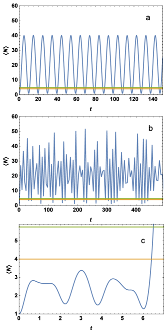
Figure 1: Plot of $\langle N\rangle$ (blue solid lines) and the invariants $E_{\rm eff}$ (green lines) and $I$ (orange lines) for the initial conditions $\langle N\rangle_{0}=1$, $\langle O_{\pm}\rangle_{0}=0$, $X_{0}=1$ and $P_{0}=-2.54950976$, with parameters $\omega=1$ and $\alpha/\Delta=0.0001$ (a), 0.015 (b) and 1.1 (c), while $\varepsilon/\Delta=1.05$ (a)–(b), and $2$ (c). Fig. 1a corresponds to the oscillatory zone and 1b to the non-linear and chaotic one. In 1c, $\langle N\rangle$ diverges for large $t$.

     

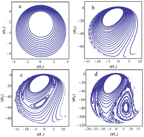
Figure 2: Poincare sections $\langle O_{+}\rangle$ vs. $\langle O_{-}\rangle$ for $X=0$, corresponding to $E_{\rm eff}=4.8$ and $I=4$, with $X_{0}=1$, $\langle N\rangle_{0}=1$, $\langle O_{+}\rangle_{0}=0$ and $\omega=1$. The values of $\langle O_{-}\rangle_{0}$ and $P_{0}$ change in order to generate the 21 curves. We set $\alpha/\Delta=0.015$ while the ratios $\varepsilon/\Delta$ are given by (a) $\varepsilon/\Delta=1.5$, (b) $\varepsilon/\Delta=1.075$, (c) $\varepsilon/\Delta=1.065$, (d) $\varepsilon/\Delta=1.05$. For decreasing values of $\varepsilon/\Delta$, the behavior evolves from periodic curves to complex quasiperiodic curves and finally to chaos.

The numerical results were obtained for initial conditions consistent with a proper density operator, such that the pertinent uncertainty relations are satisfied for all times. We have also checked their accuracy by verifying the constancy in time of the dynamical invariants $E_{\rm eff}$ and $I$ (within a precision of $10^{-10}$).

The obtained numerical results indicate that the distinct regimes obeyed by the semiclassical system are determined by the relation between $\varepsilon$, $\Delta$ and $\alpha$ irrespective of the initial conditions and the value of $\omega$. When $|\alpha|\geq\varepsilon$, the dynamics is always divergent (with or without oscillations), as occurs in the linear case, with $\alpha$ playing the role of $\Delta$. In Fig. 1 we show a characteristic evolution of $\langle N\rangle$ (together with those of the invariants, as check). When $\varepsilon>|\alpha|$, the dynamics is determined by $\varepsilon$, $\Delta$ y $\alpha$, competing $\varepsilon$ with the two coupling constants, but as $\alpha$ decreases, the system approaches the linear case and hence the relation between $\Delta$ and $\varepsilon$ becomes dominant. In Figs. 2 and 3 we show the Poincare sections obtained from the $X(t)=0$ plane, for the same values of $E_{\rm eff}$ and $I$. In Figs. 2, $\alpha<\varepsilon$ is kept fixed but the ratio $\varepsilon/\Delta$ is varied. It is seen that for $\varepsilon>|\Delta|$ the dynamics is periodic (Fig. 1a and Figs. 2a-2b) as in the linear case for most ratios, but becomes quasiperiodic (Fig. 2c) in the vicinity of the non-diagonalizable regime $\varepsilon=|\Delta|$, showing increasing nonlinear effects as this region is approached (Fig. 1b). For $\varepsilon<|\Delta|$ the regime becomes divergent as in the linear case.

Figure 3: Poincare sections $\langle O_{+}\rangle$ vs. $\langle O_{-}\rangle$ for $X=0$ as in Fig. 2, with the same inital conditions and parameter values, but setting $\varepsilon/\Delta=1.05$ (fixed) and varying $\alpha/\Delta$: (a) $\alpha/\Delta=0.0001$, (b) $\alpha/\Delta=0.01$, (c) $\alpha/\Delta=0.015$. For increasing values of $\alpha/\Delta$, the behavior evolves again from periodic curves to complex quasiperiodic curves and finally to chaos. Fig. (c) coincides with Fig. 2 (d).

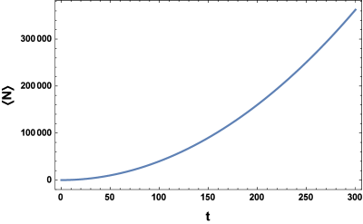
Figure 4: $\langle N\rangle$ vs. $t$. The initial conditions and parameter values are those of Fig. 1, but now $\varepsilon=\Delta=1$ and $\alpha=10^{-6}$. This is the non-diagonalizable region of the linear case. For the depicted times this curve is practically similar to that of the linear case.

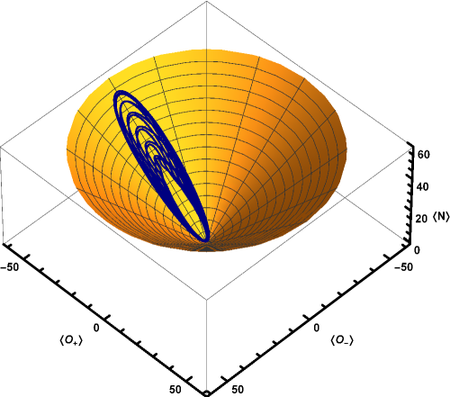
Figure 5: Solution of the subsystem (8) for one of the cuasiperiodic curves of Fig. 2d). In this case Eq. (9) represents a two-sheet hyperboloid ($I=4$).

     

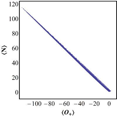
Figure 6: Poincare section $\langle N\rangle$ vs. $\langle O_{+}\rangle$ for $X=0$. This plot corresponds to Fig. 2 (d) (same initial conditions and parameter values). In the nonlinear case it is no longer a surface.

The most remarkable behavior occurs in the critical regime $\varepsilon\simeq|\Delta|$, i.e. in the vicinity of the non-diagonalizable case of the linear system, at border with the unstable case. Here we find complex quasiperiodic evolution curves (Fig. 2c). Moreover, for appropriate “small” values of $\alpha$ ($\alpha<\Delta$), chaos is seen to emerge, as shown in Fig. 2d, where the characteristic presence of chaotic see is recognized. In Figs. 3, we see the same behavior for different values of $\alpha<\varepsilon$, maintaining the same ratio $\varepsilon/\Delta$. Fig. 3c, coincides with Fig. 2d. The existence of chaos was verified by the calculation of the Lyapunov characteristic exponent, which is positive for the curves in question. On the other hand, the linear regime is approached when $\alpha$ decreases (Fig. 4). Here we have $\varepsilon=\Delta$ for $\alpha=10^{-6}$. The result is practically the same as in the linear case (Eq. (18)).

Eq. (9) represents different types of surfaces in the space $(\langle N\rangle,\langle O_{-}\rangle,\langle O_{+}\rangle)$. If $I>0$ it represents a two-sheet hyperboloid whereas for $I=0$ it is a cone. Surfaces are obviously limited by the condition $\langle N\rangle\geq 0$.

In Fig. 5, we depict a solution of subsystem (8), corresponding to a quasiperiodic curve of Fig. 2d. This solution rests on the intersection of surface $I=4$ and the region $E_{\rm eff}=4.8$. This last quantity represents a plane in the linear case ($\alpha=0$), but in the nonlinear case is no longer a surface, as seen in Fig.  6. The curves, are no longer plane, and this fact enables the onset of chaos.

IV Conclusions

In this article we have studied the dynamics of a semiquantum system resulting from the interaction of a bosonic system with a classical field. The dynamics of the bosonic version of a BCS-like pairing Hamiltonian was solved with a methodology RK.05 ; RK.09 suitable for completely general, not necessarily positive, quadratic forms. Through this methodology we found the existence of a quasi-periodic regime, a divergent regime and an intermediate regime that corresponds to a non-diagonalizable (i.e., non-separable) case. These zones are determined by the relation between the parameter $\varepsilon$ and the quantum coupling constant $\Delta$ ( $\varepsilon>|\Delta|$, $\varepsilon<|\Delta|$, $\varepsilon=|\Delta|$ respectively) RK.05 .

This quantum Hamiltonian is coupled to a classical harmonic oscillator that represents a mode of the electromagnetic field. The coupling introduces nonlinear effects in the equations of motion. The nonlinear dynamics of the composite system is determined by $\varepsilon$ and the two coupling constants $\Delta$ and $\alpha$. If $\varepsilon\leq|\alpha|$ the dynamic is divergent (Fig. 1). If $\varepsilon>|\alpha|$, it will depend on the relation between the three constants, competing $\varepsilon$ with the two coupling constants. The dynamics can be periodic, quasi-periodic and also complex and even chaotic as is observed in Figs. 2-3. In these figures Poincare sections are shown for fixed values of the effective energy $E_{\rm eff}$ and of the invariant of motion $I$, together with the plane $X=0$. When $\alpha$ tends to zero, the relationship between $\varepsilon$ and $\Delta$ of the linear case is recovered. In Fig. 4 this situation is observed for a case corresponding to a non-diagonalizable linear regime.

The most remarkable behavior occurs for specific small finite values of $\alpha$. In this case, in the vicinity of the non-diagonalizable linear regime ($\varepsilon\simeq\Delta$), we can observe the emergence of chaos (Figs. 2d -3c). This result was tested by the calculation of the pertinent Lyapunov characteristic exponent, which is positive for these curves.

We can conclude that the use of the aforementioned methodology has facilitated the analysis of the dynamics of the semiquantal nonlinear system through that of the associated linear subsystem. It has also allowed us to understand the appearance of the chaotic phenomenon by its relation to the non-diagonalizable linear case. Although the presence of the classical system enables the existence of chaos, the previous fact allows us to visualize this effect as a phenomenon emerging from the quantum system.

Acknowledgment. The authors acknowledge support from CIC and UNLP of Argentina.

References

- (1) E. Bloch, Phys. Rev. 70, 460 (1946); 70, 474 (1946).
- (2) P. Milonni, M. Shih, J.R. Ackerhalt, Chaos in Laser-Matter Interactions, World Scientific Publishing Co., Singapore, 1987.
- (3) P. Meystre, M. Sargent, Elements of Quantum Optics, Springer, NY, 1991.
- (4) P. Ring, P. Schuck, The Nuclear Many-Body Problem, Springer-Verlag: Berlin, Germany, 1980.
- (5) R. Rossignoli, A.M. Kowalski, Phys. Rev. A 72, 032101 (2005).
- (6) R. Rossignoli, A.M. Kowalski, Phys. Rev. A 79, 062103 (2009).
- (7) A.M. Kowalski, A. Plastino, A.N. Proto, Phys. Rev. E 52, 165 (1995).
- (8) A.M. Kowalski, Physica A 458, 106 (2016).
- (9) J.P. Blaizot and G. Ripka, Quantum Theory of Finite Systems, MIT Press, MA, 1986.
- (10) E.V. Goldstein, P. Meystre, Phys. Rev. A 55, 2935 (1997).
- (11) H. Pu, N.P. Bigelow, Phys. Rev. Lett. 80, 1134 (1998); C.K. Law, H. Pu, N.P. Bigelow, J.H. Eberly, Phys. Rev. Lett. 79, 3105 (1997).
- (12) S. Alexandrov, V.V. Kavanov, J.Phys. Condens. Matter 14, L327 (2002); V.I. Yukalov and E.P. Yukalova, Laser Phys. Lett. 1, 50 (2004);
- (13) E. Fukuyama, M. Mine, M. Okumura, T. Sunaga, Y. Yamanaka, Phys. Rev. A 76, 043608 (2007); M. Mine et al, Ann. Phys. 322, 2327 (2007).
- (14) T. Sunaga et al, J. Low Temp Phys. 148, 381 (2007); M. Mine et al, J. Low Temp. Phys. 148, 331 (2007).
- (15) Y. Nakamura, M. Mine, M. Okumura, Y. Yamanaka, Phys. Rev. A 77, 043601 (2008).
- (16) V. Gurarie, J.T. Chalker, Phys. Rev. Lett. 89, 136801 (2002).
- (17) I.A. Pedrosa, Phys. Rev. A 55, 3219 (1997).
- (18) V.V. Dodonov, J. Phys. A 33, 7721 (2000).
- (19) A.M. Kowalski et al, Phys. Lett. A 297, 162 (2002).
- (20) L. Rebón, R. Rossignoli, N. Canosa, Phys. Rev. A 89, 042312 (2014).
- (21) A. Aftalion, X. Blanc, J. Dalibard, Phys. Rev. A 71, 023611 (2005); S. Stock et al, Laser Phys. Lett. 2, 275 (2005).
- (22) I. Bloch, J. Dalibard, W. Zwerger, Rev. Mod. Phys. 80, 885 (2008).
- (23) M. Linn, M. Niemeyer, A. L. Fetter, Phys. Rev. A 64, 023602 (2001).
- (24) A. L. Fetter, Phys. Rev. A 75, 013620 (2007).
- (25) M. Ö. Oktel, Phys. Rev. A 69, 023618 (2004).
- (26) A. Aftalion, X. Blanc, N. Lerner, Phys. Rev. A 79 011603(R) (2009).
- (27) H. Attias, Y. Alhassid, Nucl. Phys. A 625, 363 (1997).
- (28) R. Rossignoli, N. Canosa, Phys. Lett. B 394, 242 (1997); R. Rossignoli, N. Canosa, P. Ring, Phys. Rev. Lett. 80 1853 (1998); Phys. Rev. B 67, 144517 (2003).