RACORN-K: Risk-Aversion Pattern Matching-based Portfolio Selection

Abstract

Portfolio selection is the central task for assets management, but it turns out to be very challenging. Methods based on pattern matching, particularly the CORN-K algorithm, have achieved promising performance on several stock markets. A key shortage of the existing pattern matching methods, however, is that the risk is largely ignored when optimizing portfolios, which may lead to unreliable profits, particularly in volatile markets. We present a risk-aversion CORN-K algorithm, RACORN-K, that penalizes risk when searching for optimal portfolios. Experiments on four datasets (DJIA, MSCI, SP500(N), HSI) demonstrate that the new algorithm can deliver notable and reliable improvements in terms of return, Sharp ratio and maximum drawdown, especially on volatile markets.

Index Terms—  Risk Aversion, Portfolio Selection, Pattern Matching, RACORN-K

1 Introduction

Portfolio selection has gained much interest for its theoretical importance and practical value. It aims at optimizing the assets allocation so that higher returns can be obtained while taking less risk. According to the assumptions of the financial signal, existing portfolio selection strategies can be classified into three categories [1]: follow-the-winner [2, 3, 4, 5], follow-the-loser [6, 7, 8, 9], and pattern matching [10, 11, 12]. The first two categories heavily rely on the trend of the market, thus may lead to a huge loss if the trend is not as assumed [13]. The pattern matching approach, in contrast, relies on a more practical assumption that patterns will reoccur, hence more practically applicable.

A typical pattern matching algorithm involves two stages: similar period retrieval and portfolio optimization. Most of the existing researches focus on the first stage, in particular how to measure the similarity between the market status in the past and that at present. For example, Gyorfi et al. [10, 11] uses Euclidean distance, while Li et al. [12] adopts the Pearson correlation coefficient. Empirical studies demonstrate that the correlation-based pattern matching approach, denoted by CORN-K, can generally achieve better performance than other pattern matching-based methods [12].

In spite of the success of CORN-K (and some other pattern matching methods), a potential problem of this approach is that no risk is considered when searching for optimal portfolios, i.e., the second stage of the algorithm. This is clearly a shortcoming as risky portfolios will lead to reduced long-term return. This problem is particularly severe for volatile markets that involve many risky assets. A natural idea is to penalize the risky portfolios when searching for the optimal portfolio. In this work, we propose a risk-aversion CORN-K algorithm, RACORN-K, that penalizes risky portfolios by adding a regularization term in the optimization objective function. We evaluate this new algorithm with four datasets (DJIA, MSCI, SP500(N), HSI). The results demonstrate that RACORN-K delivers notable and consistent performance improvements, in terms of long-term return, Sharp ratio and maximum drawdown. The improvements on the volatile markets DJIA and SP500(N) are particularly remarkable, demonstrating the value of the proposal.

2 Problem Setting

Consider an investment over $m$ assets on $n$ trading periods. Define the relative price vector at trading period $t$ by $\mathbf{x}_{t}=(x_{t,1},...,x_{t,m})\in\mathbb{R}^{m}_{+}$, whose $i$-th component $x_{t,i}=\frac{P(t,i)}{P(t-1,i)}$ and $P(t,i)$ is the closing price of the $i$-th asset at the $t$-th trading period. Given a window size $w$, the market window for period $t$ is defined as $\mathbf{X}^{t-1}_{t-w}=(\mathbf{x}_{t-w},...,\mathbf{x}_{t-1})$, which is assumed to represent the status of the market at period $t$.

A portfolio denoted by $\mathbf{b}_{t}=(b_{t,1},...,b_{t,m})^{T}\in\mathbb{R}^{m}$ is defined as a distribution over the $m$ assets, where $b_{t,i}$ is the proportion of the investment on the $i$-th asset at period $t$. In this study, we assume that only long positions are allowed, which implies the following constraint on $\mathbf{b}_{t}$: $b_{t,i}\geq 0,\sum_{i}b_{t,i}=1$.

At the trading period $t$, an investor selects a portfolio $\mathbf{b}_{t}$ given the past market relative prices $\{\mathbf{x}_{1},...,\mathbf{x}_{t-1}\}$. The instant return is computed by $s_{t}=\sum_{i}b_{t,i}x_{t,i}=\mathbf{b}_{t}^{T}\mathbf{x}_{t}$, and the accumulated return produced by $\{\mathbf{b}_{1},...,\mathbf{b}_{n}\}$ is $S_{t}=\prod_{j=1}^{n}\mathbf{b}_{j}^{T}\mathbf{x}_{j}$.

3 Algorithm

In this section, we first give a brief description of the classical CORN-K algorithm, and then propose our RACORN-K algorithm. A conservative version of RACORN-K, denoted by RACORN(C)-K, will be also proposed.

3.1 CORN-K algorithm

At the $t$-th trading period, the CORN-K algorithm first selects all the historical periods whose market status is similar to that of the present market, where the similarity is measured by the Pearson correlation coefficient. This patten matching process produces a set of similar periods, denoted by $C(\mathbf{x}_{t};w,\rho)$, where $w$ is the size of the market window, and $\rho$ is the threshold when selecting similar periods. This is formulated as follows:

$$C(\mathbf{x}_{t};w,\rho)=\{\mathbf{x}_{j}|corr(\mathbf{X}^{j-1}_{j-w},\mathbf{X}^{t-1}_{t-w})>\rho\},$$

where $corr(X,Y)$ is the correlation coefficient between $X$ and $Y$, and $w<j<t$. Note that when calculating the correlation coefficient, the columns in $\mathbf{X}^{j-1}_{j-w}$ (the same for $\mathbf{X}^{t-1}_{t-w}$) are concatenated into a $(m\times w)$-dimensional vector. Once the similar periods have been selected, the portfolio on the $m$ assets can be obtained following the BCRP principle [14]:

$$\mathbf{b}^{*}_{t}(w,\rho)=\mathop{argmax}_{\mathbf{b}\in\Delta_{m}}\sum_{\mathbf{x}\in C(\mathbf{x}_{t};w,\rho)}log(\mathbf{b}^{T}\mathbf{x}),$$ (1)

where $\Delta_{m}=\{\mathbf{b}:\sum_{i=1}^{m}b_{i}=1,b_{i}\geq 0\}$ represents a simplex with $m$ components.

Finally, CORN-K selects various $w$ and $\rho$. By each setting of these parameters $(w,\rho)$, an optimal portfolio $\mathbf{b}^{*}_{t}(w,\rho)$ is computed following (1). Note that $\mathbf{b}^{*}_{t}(w,\rho)$ is a particular strategy, also called an ‘expert’, denoted by $\epsilon(w,\rho)$. The experts which achieve top-k accumulated returns are selected to compose an expert ensemble $E_{t}$, where the accumulated return of an expert $\epsilon(w,\rho)$ is denoted by $S_{t}(w,\rho)$. With the expert ensemble $E_{t}$, the ensemble-based optimal portfolio is derived by:

$$\mathbf{b}^{*}_{t}=\frac{\sum_{\epsilon(w,\rho)\in E_{t}}S_{t-1}(w,\rho)\mathbf{b}^{*}_{t}(w,\rho)}{\sum_{\epsilon(w,\rho)\in E_{t}}S_{t-1}(w,\rho)}.$$ (2)

It is expected that this ensemble-based average leads to more robust portfolios.

3.2 Risk-Aversion CORN-K (RACORN-K)

The portfolio optimization is crucial for the success of CORN-K. A potential problem of the existing form (1), however, is that the optimization is purely profit-driven. This is clearly dangerous as the high-profit assets it selects may exhibit high variation, leading to a risky portfolio that suffers from unexpected loss. It is particularly true for volatile markets where the prices of many assets are unstable. A natural idea to solve this problem is to penalize risky portfolios when searching for the optimal portfolio. This leads to a risk-aversion CORN-K, denoted by RACORN-K. More specifically, the objective function in (1) is augmented by a risk-penalty term, formulated as follows:

$$\mathbf{b}^{*}_{t}(w,\rho,\lambda)=\mathop{argmax}_{\mathbf{b}\in\Delta_{m}}\frac{\sum_{\mathbf{x}\in C(\mathbf{x}_{t};w,\rho)}log(\mathbf{b}^{T}\mathbf{x})}{|C(\mathbf{x}_{t};w,\rho)|}-\lambda\sigma_{t}(w,\rho)$$ (3)

where $\lambda$ is the risk-aversion coefficient, $|C(\mathbf{x}_{t};w,\rho)|$ is the size of $C(\mathbf{x}_{t};w,\rho)$ , and $\sigma_{t}(w,\rho)$ is the risk:

$$\sigma_{t}(w,\rho)=std(log(\mathbf{b}^{T}\mathbf{x}))|_{\mathbf{x}\in C(\mathbf{x}_{t};w,\rho)},$$

where $std(\cdot)$ denotes the standard deviation function.

We emphasize that the risk-penalty term $std(log(\mathbf{b}^{T}\mathbf{x}))$ is different from $\mathbf{b}^{T}std(log(\mathbf{x}))$: the former is the risk of the portfolio, while the latter is the sum of the risk of the assets according to the portfolio. This form is similar to the classical mean-variance model [15]. A key difference from the mean-variance model (and most other risk-aversion models) is that the risk is computed over the historical price relatives in $C(\mathbf{x}_{t};w,\rho)$, rather than on the whole trading periods. It therefore estimates the risk of the portfolio with a particular pattern matching strategy, i.e., the CORNK-K algorithm, rather than the unconstrained market risk of the selected assets.

With the new optimization objective (3), the ensemble-based optimal portfolio is derived similarly as in CORN-K. The only difference is that we have introduced a new hyper-parameter $\lambda$, so the expert should be extended to $\epsilon(w,\rho,\lambda)$. The derivation is similar to (2), formulated by:

$$\mathbf{b}^{*}_{t}=\frac{\sum_{\epsilon(w,\rho,\lambda)\in E_{t}}S_{t-1}(w,\rho,\lambda)\mathbf{b}^{*}_{t}(w,\rho,\lambda)}{\sum_{\epsilon(w,\rho,\lambda)\in E_{t}}S_{t-1}(w,\rho,\lambda)}.$$

3.3 Conservative RACORN-K (RACORN(C)-K)

In the above RACORN-K algorithm, the risk-aversion coefficient $\lambda$ is treated as a new free parameter and is combined with $w$ and $\rho$ to derive ensemble-based optimal portfolio. A potential problem of this type of ‘naive ensemble’ is that it does not consider the time-variant property of the risk. In fact, the risk of the portfolio derived from each expert tends to change quickly in an volatile market and therefore the weights of individual experts should be adjusted timely. To achieve the quick adjustment, we use the instant return $s_{t}(w,\rho,\lambda)$ to weight the experts with different $\lambda$, rather than the accumulated return $S_{t-1}(w,\rho,\lambda)$. This is formulated as follows:

$$\mathbf{b}^{*}_{t}(w,\rho)=\frac{\sum_{\lambda}s_{t}(w,\rho,\lambda)\mathbf{b}^{*}_{t}(w,\rho,\lambda)}{\sum_{\lambda}s_{t}(w,\rho,\lambda)}.$$ (4)

Since $s_{t}$ is not available when estimating $\mathbf{b}^{*}_{t}$, we approximate it by the geometric average of the returns achieved in $C(\mathbf{x}_{t};w,\rho)$, given by:

$$s_{t}(w,\rho,\lambda)\approx exp(\frac{\sum_{\mathbf{x}_{j}\in C(\mathbf{x}_{t};w,\rho)}log(\mathbf{b}_{t}^{*}(w,\rho,\lambda)^{T}\mathbf{x}_{j})}{|C(\mathbf{x}_{t};w,\rho)|}).$$

In practice, we find that omitting the normalization term $\frac{1}{|C(\mathbf{x}_{t};w,\rho)|}$ can deliver slightly better results.

Once $\mathbf{b}^{*}_{t}(w,\rho)$ is obtained, the ensemble-based optimal portfolio can be derived as CORN-K following (2), where the accumulated return $S_{t-1}(w,\rho)$ is achieved by applying the portfolios derived by (4). Compared to RACORN-K, this variant algorithm is more risk-aware and thus assumed to be more conservative. We denote this conservative version of RACORN-K as RACORN(C)-K.

4 Experiments

We evaluate RACORN-K and RACORN(C)-K on four datasets, and compare the performance with the classical CORN-K algorithm. The performances of some other popular strategies are also reported.

4.1 Dataset

Table 1: Datasets used in the experiments.

Dataset	Region	Time range	Trading days	Assets
DJIA	US	2001/01/14 - 2003/01/14	507	30
MSCI	GLOBAL	2006/04/01 - 2010/03/31	1043	24
SP500(N)	US	2000/01/03 - 2014/12/31	3773	10
HSI	HK	2000/01/03 - 2014/12/31	3702	10

Table 1 shows the four datasets used in our experiments. The DJIA (Dow Jones Industrial Average) dataset is a collection of $30$ large publicly owned companies based in the United States, collected by Borodin et al. [6]. The MSCI dataset is a collection of $24$ global equity indices which are the constituents of MSCI World Index. These two datasets are relatively old. In order to evaluate the performance of the proposed algorithms on more recent data, we collected another two datasets: SP500(N) and HSI. The SP500(N) dataset consists of $10$ equities with the largest market capitalization (as of Apr. 2003) from the S&P 500 Index. Note that this dataset is different from the SP500 dataset collected by Li et al. [12]. The latter is a little old and may not reflect the trend of the current market. The HSI dataset contains $10$ equities with the largest market capitalization (as of Jan. 2005) from Hang Seng Index. It is worth noting that SP500(N) and HSI cover both bull markets and bear markets, particularly the finance crisis in 2009.

4.2 Implement details

The OLPS toolbox [16] is used to implement the baseline strategies, where the default values are set for the hyper-parameters. For RACORN-K, the maximum window size is set to $5$. The correlation coefficient threshold $\rho$ ranges from $0$ to $0.9$, with the step set to be $0.1$. The risk-aversion coefficient $\lambda$ ranges from $0$ to $0.03$, with a step $0.01$. While combining the outputs of experts, top 10% experts are selected to compose the ensemble $E_{t}$. As for RACORN(C)-K, all the parameters are the same as RACORN-K, except that $\lambda$ ranges from $0$ to $0.1$ with a step $0.01$, as we found RACORN(C)-K has the capability to accept a larger maximum risk aversion. These parameters are used in the experiments on all the four datasets.

4.3 Experimental results

Three metrics are adopted to evaluate the performance of a strategy: accumulated return (RET), Sharpe ratio (SR) and maximum drawdown (MDD). Among these metrics, SR and MDD are more concerned as our main goal is to control the risk. And the improvement on SR and the reduction on MDD are often more important for investors, particularly for asset managers who can leverage various financial tools to magnify returns.

Table 2: Performances of different strategies on four datasets.

	Dataset	DJIA			MSCI			SP500(N)			HSI
	Criteria	RET	SR	MDD	RET	SR	MDD	RET	SR	MDD	RET	SR	MDD
Main Results	RACORN(C)-K	0.93	0.01	0.32	78.38	3.73	0.21	12.55	0.77	0.53	202.04	1.60	0.28
	RACORN-K	0.83	-0.19	0.37	79.52	3.67	0.21	13.03	0.72	0.57	264.02	1.60	0.29
	CORN-K	0.80	-0.24	0.38	77.54	3.63	0.21	12.50	0.70	0.60	254.27	1.56	0.30
Naive Methods	UBAH	0.76	-0.43	0.39	0.90	0.02	0.65	1.52	0.24	0.50	3.54	0.53	0.58
	UCRP	0.81	-0.28	0.38	0.92	0.05	0.64	1.78	0.28	0.68	4.25	0.58	0.55
Follow the Winner	UP	0.81	-0.29	0.38	0.92	0.04	0.64	1.79	0.29	0.68	4.26	0.59	0.55
	EG	0.81	-0.29	0.38	0.92	0.04	0.64	1.75	0.28	0.67	4.22	0.58	0.55
	ONS	1.53	0.80	0.32	0.85	0.02	0.68	0.78	0.27	0.96	4.42	0.52	0.68
Follow the Loser	ANTICOR	1.62	0.85	0.34	2.75	0.96	0.51	1.16	0.24	0.93	9.10	0.74	0.56
	ANTICOR2	2.28	1.24	0.35	3.20	1.02	0.48	0.71	0.22	0.97	12.27	0.77	0.55
	PAMR_2	0.70	-0.15	0.76	16.73	2.07	0.54	0.01	-0.28	1.00	1.19	0.20	0.86
	CWMR_Stdev	0.69	-0.17	0.76	17.14	2.07	0.54	0.02	-0.26	0.99	1.28	0.22	0.85
	OLMAR1	2.53	1.16	0.37	14.82	1.85	0.48	0.03	-0.11	1.00	4.19	0.46	0.77
	OLMAR2	1.16	0.40	0.58	22.34	2.08	0.42	0.03	-0.11	1.00	3.65	0.43	0.84
Pattern Matching based Algorithms	BK	0.69	-0.68	0.43	2.62	1.06	0.51	1.97	0.31	0.59	13.90	0.88	0.45
	BNN	0.88	-0.15	0.31	13.40	2.33	0.33	6.81	0.67	0.41	104.97	1.40	0.33

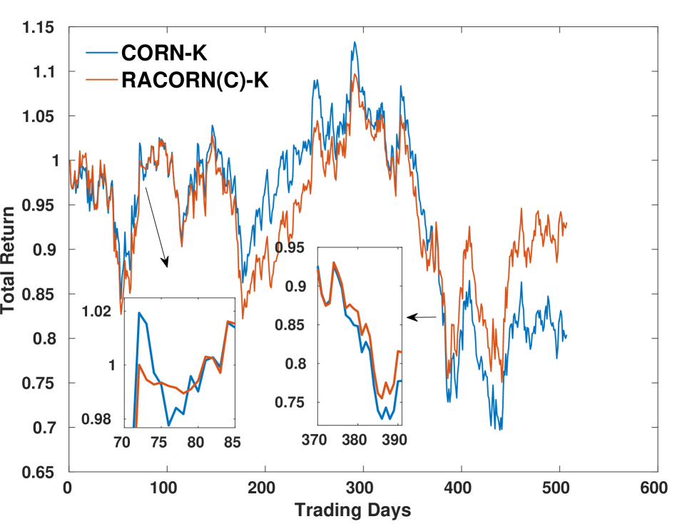
(a) DJIA

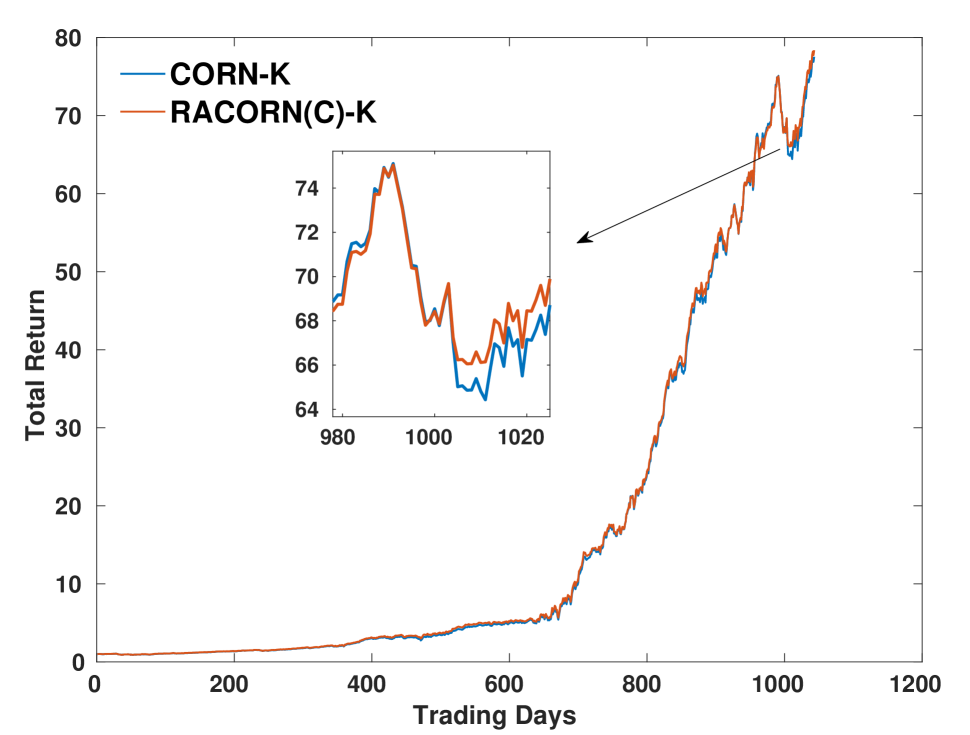
(b) MSCI

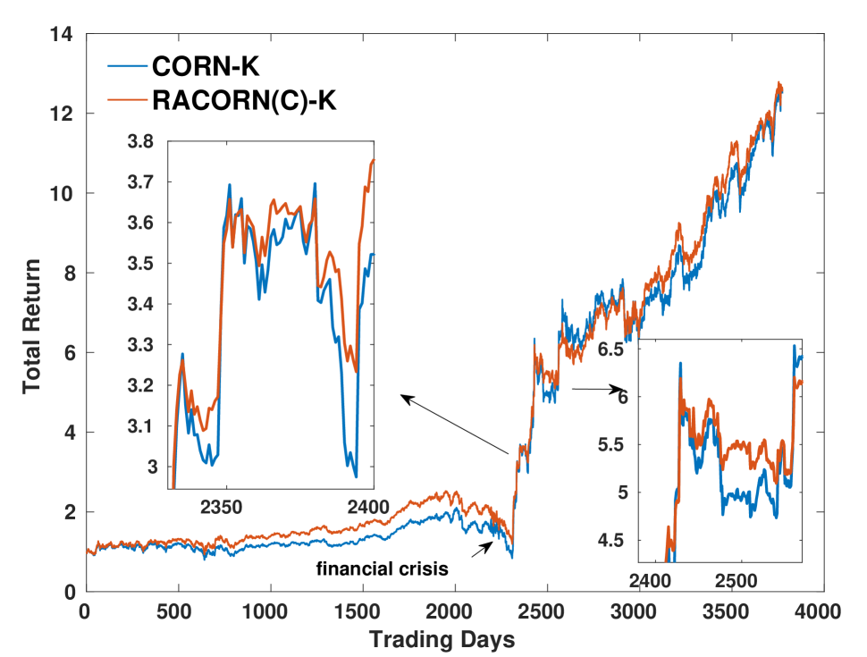
(c) SP500(N)

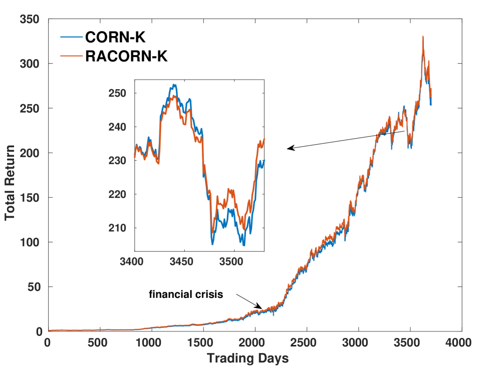
(d) HSI

Fig. 1: RET curves with CORN-K and RACORN-K/RACORN(C)-K on four datasets.

4.3.1 General results

Table 2 summarizes the results, where the improvements compared to CORN-K have been marked as bold face. From these results, it can be seen that RACORN-K consistently improves SR and MDD on all the datasets, which confirms that involving risk aversion does reduce the risk of the derived portfolio. The conservative version, RACORN(C)-K, delivers even better performance in terms of SR and MDD, though the long-term return (RET) is slightly reduced. In most cases, both RACORN-K and RACORN(C)-K obtain larger RETs than the CORN-K baseline, demonstrating that controlling risk will ultimately improve long-term profits. The only exception is that the RET on HSI drops with RACORN(C)-K; however, the absolute RET has been very high, so this RET reduction can be regarded as a reasonable cost for the risk control.

Fig. 1 shows the RET curves with CORN-K and RACORN-K/RACORN(C)-K. It can be seen that RACORN-K or RACORN(C)-K has the same trend as CORN-K in general, particularly on relatively stable markets (MSCI and HSI). However, in periods where CORN-K is risky, RACORN(C)-K behaves less bumpy and hence more reliable. This can be seen clearly in (a) DJIA and (c) SP500(N). Fig. 1 presents some ‘key points’ where RACORN(C)-K behaves more ‘smooth’ than CORN-K. Due to this smoothness, the risk of the strategy is reduced, and extremely poor trading can be largely avoided.

When comparing to other baselines, it can be seen that the CORN-K family performs much better and more consistent. For example, OLMAR1, a classical follow-the-loser strategy, performs the best on DJIA, but the advantage is totally lost on other datasets. These results re-confirm the reliability of pattern matching methods.

4.3.2 Detailed analysis

Analyzing the performance of RACORN-K/RACORN(C)-K on different markets sheds more light on the property of the risk-aversion approach. From Table 2, we can see that RACORN-K/RACORN(C)-K obtains the most significant SR improvement on DJIA, and the most significant MDD reduction on DJIA and SP500(N). Interestingly, these two datasets are the ones that the conventional CORN-K does not work well (less RET, smaller SR, higher MDD). This can be also seen from Fig. 1, where the RET curves with CORN-K exhibit more risk on DJIA and SP500(N) compared to the curves on MSCI and HSI. This indicates that RACORN-K/RACORN(C)-K are more effective when the conventional CORN-K is risky.

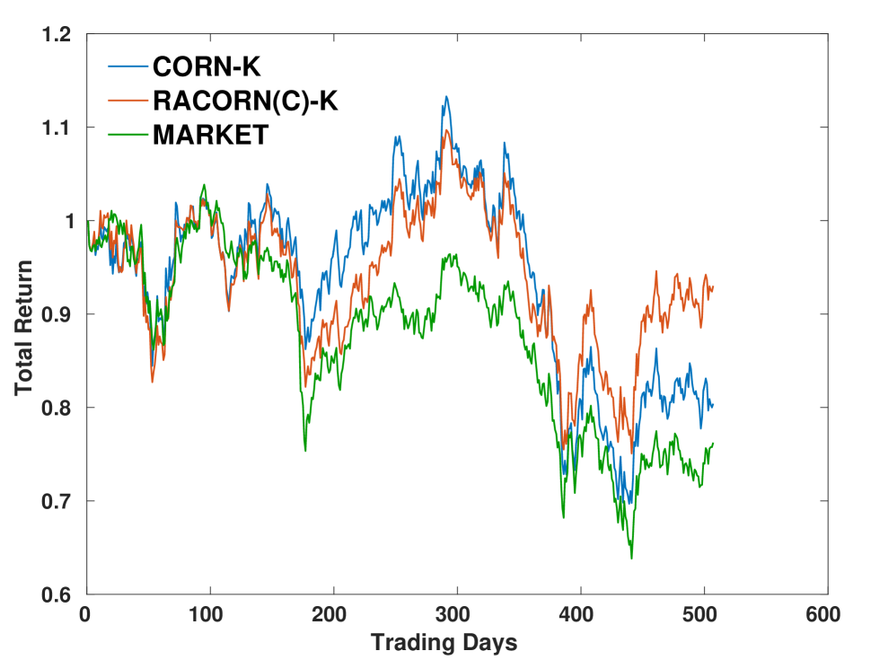
(a) DJIA

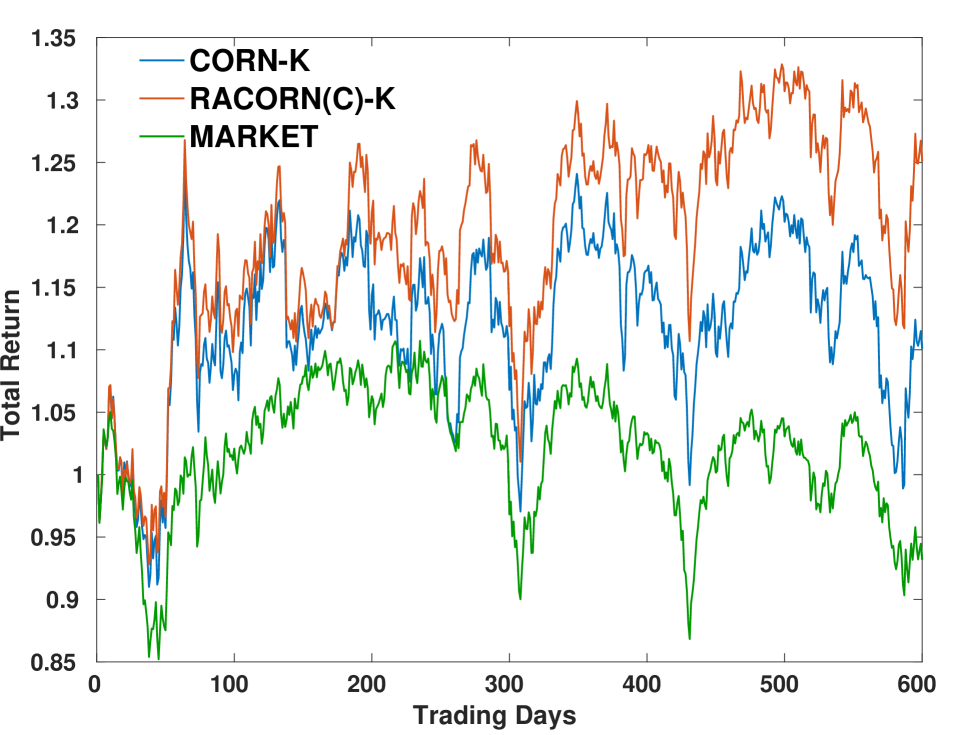
(b) SP500(N)

Fig. 2: Market and RET curves with CORN-K and RACORN(C)-K on DJIA and SP500(N).

More analysis shows that the risk of CORN-K is largely attributed to the risk of the market. To make it clear, the market returns of DJIA and SP500(N) are plotted together with the RET curves of CORN-K and RACORN(C)-K in Fig. 2. For a clear presentation, only the first 600 trading days of SP500(N) are plotted as during this period the market is volatile. It shows clearly that on the markets with huge volatility, involving risk-aversion largely reduced the risk, hence a more reliable strategy. As a summary, CORN-K may perform less effective on risky markets, and the risk-aversion algorithms can largely alleviate this problem. Fortunately, this advantage on risky markets does not degrade its performance on stable markets (where CORN-K works well). This is a nice property and indicates that RACORN-K/RACORN(C)-K is a safe and effective extension/substitution of CORN-K.

5 Conclusion

This paper presented two risk-aversion CORN-K algorithms, RACORN-K and RACORN(C)-K that involve a risk-aversion penalty when searching for optimal portfolios. Experimental results on four datasets demonstrate that the new algorithms can consistently improve the Sharpe ratio and reduce maximum drawdown. This improvement is particularly significant on high-risk markets where the conventional CORN-K tends to perform not as well. Fortunately, this risk control does not degrade the long-term profit in general, and in many cases, it leads to even better returns. Future work involves exploring more suitable regularizations, e.g., group penalty and temporal continuity constraint.

References

- [1] Bin Li and Steven CH Hoi, “Online portfolio selection: A survey,” ACM Computing Surveys (CSUR), vol. 46, no. 3, pp. 35, 2014.
- [2] Thomas M Cover, “Universal portfolios,” Mathematical finance, vol. 1, no. 1, pp. 1–29, 1991.
- [3] David P Helmbold, Robert E Schapire, Yoram Singer, and Manfred K Warmuth, “On-line portfolio selection using multiplicative updates,” Mathematical Finance, vol. 8, no. 4, pp. 325–347, 1998.
- [4] Amit Agarwal, Elad Hazan, Satyen Kale, and Robert E Schapire, “Algorithms for portfolio management based on the newton method,” in Proceedings of the 23rd international conference on Machine learning. ACM, 2006, pp. 9–16.
- [5] Yoram Singer, “Switching portfolios,” International Journal of Neural Systems, vol. 8, no. 04, pp. 445–455, 1997.
- [6] Allan r, Ran El-Yaniv, and Vincent Gogan, “Can we learn to beat the best stock.,” J. Artif. Intell. Res.(JAIR), vol. 21, pp. 579–594, 2004.
- [7] Bin Li, Peilin Zhao, Steven CH Hoi, and Vivekanand Gopalkrishnan, “Pamr: Passive aggressive mean reversion strategy for portfolio selection,” Machine learning, vol. 87, no. 2, pp. 221–258, 2012.
- [8] Bin Li, Steven CH Hoi, Peilin Zhao, and Vivekanand Gopalkrishnan, “Confidence weighted mean reversion strategy for online portfolio selection,” ACM Transactions on Knowledge Discovery from Data (TKDD), vol. 7, no. 1, pp. 4, 2013.
- [9] Bin Li, Steven CH Hoi, Doyen Sahoo, and Zhi-Yong Liu, “Moving average reversion strategy for on-line portfolio selection,” Artificial Intelligence, vol. 222, pp. 104–123, 2015.
- [10] László Györfi, Gábor Lugosi, and Frederic Udina, “Nonparametric kernel-based sequential investment strategies,” Mathematical Finance, vol. 16, no. 2, pp. 337–357, 2006.
- [11] László Györfi, Frederic Udina, and Harro Walk, “Nonparametric nearest neighbor based empirical portfolio selection strategies,” Statistics & Decisions International mathematical journal for stochastic methods and models, vol. 26, no. 2, pp. 145–157, 2008.
- [12] Bin Li, Steven CH Hoi, and Vivekanand Gopalkrishnan, “Corn: Correlation-driven nonparametric learning approach for portfolio selection,” ACM Transactions on Intelligent Systems and Technology (TIST), vol. 2, no. 3, pp. 21, 2011.
- [13] Narasimhan Jegadeesh, “Evidence of predictable behavior of security returns,” The Journal of finance, vol. 45, no. 3, pp. 881–898, 1990.
- [14] Thomas M Cover and David H Gluss, “Empirical bayes stock market portfolios,” Advances in applied mathematics, vol. 7, no. 2, pp. 170–181, 1986.
- [15] Harry M. Markowitz, “Portfolio selection: Efficient diversification of investments, 2nd edition,” Monograph, vol. 35, no. 1, pp. 243–265, 1991.
- [16] B Li, D Sahoo, and SCH Hoi, “Olps: A toolbox for online portfolio selection,” Journal of Machine Learning Research (JMLR), 2015.