Var-CNN: A Data-Efficient Website Fingerprinting Attack Based on Deep Learning

Abstract

In recent years, there have been several works that use website fingerprinting techniques to enable a local adversary to determine which website a Tor user visits. While the current state-of-the-art attack, which uses deep learning, outperforms prior art with medium to large amounts of data, it attains marginal to no accuracy improvements when both use small amounts of training data. In this work, we propose Var-CNN, a website fingerprinting attack that leverages deep learning techniques along with novel insights specific to packet sequence classification. In open-world settings with large amounts of data, Var-CNN attains over 1% higher true positive rate (TPR) than state-of-the-art attacks while achieving $4\times$ lower false positive rate (FPR). Var-CNN’s improvements are especially notable in low-data scenarios, where it reduces the FPR of prior art by 3.12% while increasing the TPR by 13%. Overall, insights used to develop Var-CNN can be applied to future deep learning based attacks, and substantially reduce the amount of training data needed to perform a successful website fingerprinting attack. This shortens the time needed for data collection and lowers the likelihood of having data staleness issues.

1 Introduction

Due to increases in mass surveillance and other attacks on privacy, many Internet users have turned to Tor [11] to protect their anonymity. Over the years, Tor has grown to over 6,000 volunteer servers and 4 million daily users [9]. Tor protects its users’ identities by routing each packet through a number of Tor servers. Each server learns only the immediate hop before and after itself, and as a result, no single server learns both the identity of the user and the destination of the packet.

Unfortunately, Tor does not provide anonymity against a powerful global adversary who can monitor a significant portion of the traffic due to traffic analysis attacks. In such attacks, the adversary monitors traffic entering and leaving the Tor network. Then, she uses traffic patterns such as packet sequences to correlate packets across the two ends of the network and determine the identities of the two communicating parties. Recently, a variant of the traffic analysis attack called the website fingerprinting (WF) attack allows an adversary who observes only the connection between the user and the Tor network to identify which website the user visits. To do so, the adversary first learns the traffic patterns of certain websites, creating a unique digital fingerprint for each site. Then, the adversary compares these fingerprints to a user’s network traffic (typically using machine learning algorithms) to determine which website the user visits.

Most prior WF attacks [7, 40, 19, 30, 18, 4, 32, 43, 34, 16, 44, 35, 6] use manually extracted features to carry out the attack. That is, the attacker carefully studies different protocols such as HTTP and Tor, and manually determines features that could potentially identify a website from a network trace (e.g., the total number of packets and the total transmission time). While these attacks achieved good accuracy in many settings, it remains difficult to generalize the attacks across different protocols or reason about their strengths, since the attacker must manually specify the features.

Recently, deep learning neural networks have become the state-of-the-art machine learning technique in several different domains such as Computer Vision and Natural Language Processing [28]. While they can take in standard manually extracted features, one of their main advantages is their ability to automatically learn salient features just by analyzing input and output pairs. This provides them the opportunity to discover more powerful features than previously known, achieving higher accuracy. Current state-of-the-art WF attacks [36, 38] indeed outperform prior manual feature extraction attacks in settings with sufficient amounts of data.

One significant drawback of deep learning, however, is that it generally requires a large amount of training data. As a result, deep learning WF attacks have struggled to outperform traditional WF attacks in low-data scenarios. The current best deep learning WF model by Sirinam et al., for example, achieves similar results as CUMUL, the state-of-the-art manual feature extraction attack, when both use small amounts of training data [38]. Performance issues in low-data scenarios can be a serious issue for WF attacks: since website traces change quickly (i.e., in the span of a few hours to a few days), the attacker must frequently update her database of traces to match user traffic [24]. Consequently, the adversary naturally needs to be stronger to collect the larger amounts of traces required for deep learning based attacks, which weakens the attack in practice.

1.1 Our Contributions

In this work, we focus on answering the following question:

Can deep learning WF attacks achieve improved accuracy over prior state-of-the-art WF attacks even with small amounts of training data?

We answer this question affirmatively using our new attack called Var-CNN, a semi-automated feature extraction (i.e., benefitting from both manual feature extraction and automated feature extraction) WF attack based on deep learning. To the best of our knowledge, Var-CNN is the first deep learning WF attack specifically tailored to network packet sequence classification. Var-CNN’s base architecture uses ResNets [17], state-of-the-art convolutional neural networks (CNNs) in Computer Vision. Beyond the standard model architecture, Var-CNN uses the following key insights about the nature of packet sequences to achieve high performance:

1. Packet sequences have a fundamentally different structure than images or other datasets traditionally classified using CNNs. For instance, numerical digits in the MNIST [29] dataset are composed of individual edges that can be detected by small feature detectors. Packets, on the other hand, typically have a more intertwined, global relationship (e.g., packets at the beginning of a trace can cause a large ripple effect throughout the whole trace). Unfortunately, simply increasing the size of individual feature detectors results in an unwieldy increase in the computational and memory overhead. Instead, we explore the use of dilated causal convolutions, a variation found in Audio Synthesis [42] and Computational Biology [15] research, to exponentially increase feature detector size without increasing runtime (§4.3).

2. Unlike Computer Vision model inputs, which are highly abstract, network packet sequences naturally leak some cumulative statistical information such as the total number of packets, total time, etc. Although these manually extracted cumulative features achieve poor standalone accuracy, we overcome this problem by combining them with our dilated ResNet during training rather than after. This allows Var-CNN to be the first deep learning WF attack that combines both manually extracted and automatically extracted features to improve the model’s overall performance (§4.4).

3. To the best of our knowledge, packet timing information has only been used minimally in prior art WF attacks. In contrast, the input generality and power from ResNets and dilated causal convolutions allow us to retain performance under a domain change from direction information to packet timing information, showing that timing leaks a significant amount of information (§4.5). Moreover, we show that combining the direction and timing information of a packet sequence results in a more accurate overall model (§4.6).

By incorporating the above three insights into Var-CNN, we achieve substantial improvements over prior art in both the open- and closed-world in every experimental scenario tested. For instance, with 900 monitored sites and 2500 monitored traces per site in our largest closed-world, Var-CNN improves prior art accuracy from 96.5% to 98.8%. In our largest open-world setting tested, Var-CNN attains over a 1% better true positive rate (TPR) than prior art while achieving a $4\times$ lower false positive rate (FPR).

In addition, Var-CNN has significant improvements over prior art in settings with small amounts of training data, making the WF attack easier to carry out by weaker attackers. For instance, with 100 traces for each of 100 monitored sites in a low-data closed-world, Var-CNN achieves 97.8% accuracy, whereas it would take prior art $5\times$ as much training data to achieve a comparable accuracy of 98.1%. In a low-data open-world with just 60 monitored traces and 6000 unmonitored training traces, Var-CNN reduces prior-art FPR by 3.12% while increasing TPR by 13%. In §6.2, we provide an intuitive explanation for why Var-CNN works well in these settings. Moreover, although we used ResNets here as our baseline CNN architecture, many of our insights are architecture-independent and thus can be applied to any future deep learning-based attack.

2 Background and threat model

Fig. 1: The website fingerprinting threat model.

Tor [11] consists of decentralized volunteer servers that relay their users’ packets without any delays or cover traffic. While this has allowed Tor to scale to a large number of users, this also enables adversaries monitoring traffic entering and leaving the Tor network to potentially deanonymize users. In particular, the website fingerprinting (WF) threat model allows an adversary to monitor just the connection between a user and the network, as shown in Figure 1. The adversary is a passive observer, meaning she will not drop, modify, or insert any packets. Examples of such adversaries include routers, internet service providers, autonomous services, and compromised Tor servers.

The adversary is interested in identifying visitors of a number of websites, which we call monitored websites; we call all other websites unmonitored websites. The adversary visits the websites on her own and creates a database of traces, sequences of packets and their timestamps generated while visiting a website. From here on, we refer to whether a packet was incoming or outgoing as direction data and the time delay between two consecutive packets as time data. Once the database is created, the adversary monitors and collects users’ traces and uses the database to classify them as belonging to either the monitored or unmonitored set of websites.

2.1 Attacker settings

We consider two different attacker settings, closed-world and open-world.

Closed-world. In this setting, we assume that users only visit a well-known set of monitored websites. Here, the adversary trains on a number of traces from these sites and aims to classify different traces from the training set into one of the monitored websites. We use accuracy to define the effectiveness of the attacker, which is simply the proportion of monitored traces correctly identified. Although the closed-world is less realistic—it assumes the adversary knows every site a user visits—it is a useful measure of a classifier’s ability to distinguish between websites.

Open-world. In the real world, users can visit websites that the adversary does not know. Open-world settings emulate this scenario by allowing users to visit both monitored and unmonitored websites (i.e., websites that the adversary does not deem sensitive). Just like in the closed-world, the adversary trains on different traces from those being tested on. In addition, the adversary can bias her classifier by training on some number of unmonitored sites. Though there is no overlap between unmonitored training and testing sites, learning how to distinguish one set of unmonitored sites often helps with others, as we will see empirically in §5.2.4.

In the open-world setting, we use three metrics to measure classification performance, two-class true positive rate (Two-TPR), multi-class true positive rate (Multi-TPR), and false positive rate (FPR). Two-TPR is the proportion of monitored traces correctly classified as any monitored site, and it applies to an adversary who only cares about identifying users who visit the monitored class in general. Multi-TPR is the ratio of monitored traces correctly classified as a specific monitored site. An adversary using this metric might assign different penalties to different monitored sites. Finally, FPR, the ratio of unmonitored traces incorrectly classified as a monitored site, measures the adversary’s level of false identification.

2.2 Assumptions

Prior WF attacks and Var-CNN assume the following [24]:

• Replicability. Given the uncertainty of real user conditions, the WF attacker assumes her training data will be representative of actual Tor traffic sequences.

• Applicability. The adversary assumes she can apply the WF attack effectively in practice.

There are, however, several criticisms regarding these assumptions. First, the replicability assumption may be too strong for a few reasons:

1. Unless sites with dynamic content changes such as AJAX or Javascript are adequately represented in the training set, the adversary would believe a non-static page is actually static.

2. Training on one Tor Browser version while a user uses a different version could possibly result in different underlying protocols being used.

3. Varying latency in Tor connections causes different inter-packet timings.

4. The types of websites the adversary trains on may not match the types of websites real users visit. For instance, the adversary might train her classifier on Alexa’s most popular sites [1] whereas real Tor users might visit more private sites.

Second, the applicability assumption faces the following issues:

1. The adversary might not know when traffic from one website starts or stops, or whether a user visits multiple websites at the same time.

2. Noise traffic (e.g., from listening to music or downloading a file in the background) might confuse an attacker.

While some work has been done in applicability such as learning how to split traces and remove background noise [45], there remain important problems in replicability due to the privacy concerns of collecting realistic datasets from actual Tor users. Our work does touch upon the replicability concern of data freshness with dynamic websites, showing that deep learning attacks can perform well with small amounts of training data. However, we acknowledge that, similar to most prior work on WF attacks [35, 12, 6, 44, 43, 34, 16], there still exist replicability and applicability assumptions that could make the WF attack less powerful in practice.

3 Related work

We now describe prior work in greater detail.

3.1 Manual feature extraction attacks

In the past, several WF attacks with manually extracted features have been proposed, each directing attention towards the susceptible components of the protocol studied [7, 40, 19, 30, 18, 4, 32, 35, 12, 6, 44, 43, 34, 16]. For example, early work used weaknesses in HTTP 1.0 to take advantage of distinct resource length leakage, such as the size of images, scripts, and videos [7, 40, 19]. Subsequent protocols hid resource lengths, so later attacks focused instead on extracting information from packet lengths leaked by HTTP 1.1, VPNs, and SSH tunneling [30, 18, 4, 32]. Since then, Tor and other anonymous networks that hide packet lengths have emerged. Consequently, attacks in the last few years have focused on using a broad set of manually extracted features [35, 12, 6, 44]. For example, Wang et al. used a modified $k$-Nearest Neighbors ($k$-NN) classifier with a weight adjustment system to effectively train on a wide feature set [43], including packet lengths, packet orderings, packet concentrations, and bursts. Panchenko et al. developed CUMUL, a Support Vector Machine (SVM) that mainly relied on cumulative packet length features [34]. Finally, Hayes et al. in their $k$-FP attack used a slightly smaller feature set than Wang et al. and fed it into a Random Forest classifier, an ensemble of Decision Trees [16]. After training the Random Forest, they fed the output into a vanilla $k$-NN classifier to control TPR and FPR. Currently, Panchenko et al.’s CUMUL [34] is the best performing manual feature extraction attack in vanilla WF settings, achieving 97.3% accuracy in a small closed-world with a large number of traces [38].

While manual feature extraction attacks work well in some settings, they are fundamentally restricted by their feature set. For instance, Hayes et al. pointed out that since CUMUL primarily relies on packet ordering, it suffers significant decreases in accuracy against simple defenses that perturb this information [16]. In addition, even though a broad feature set as in Hayes et al.’s $k$-FP [16] and Wang et al.’s $k$-NN [43] mitigates information loss to a defense, these attacks are still only as good as their feature set. For instance, while neither could effectively use timing, our model achieves a non-trivial increase in performance when incorporating timing. This exemplifies how difficult it can be for humans to manually extract features.

3.2 Automated feature extraction attacks

Recently, a few authors have proposed work on automated feature extraction (AFE) WF attacks using deep learning neural networks [3, 36]. Compared to traditional attacks, these attacks perform AFE over raw input sequences, removing the need for feature design. In an earlier work, Abe and Goto [3] used a stacked-denoising autoencoder (SDAE), a neural network that tries to create a compressed version of its input, to perform AFE. Their model performed worse than Wang et al.’s $k$-NN with manual features. Later, Rimmer et al. [36] studied preliminary applications of SDAEs, recurrent neural networks (RNNs), and convolutional neural networks (CNNs) and showed that AFE models can slightly outperform prior art when using large amounts of training data.

The current state-of-the-art WF attack is Sirinam et al.’s [38] Deep Fingerprinting (DF) attack, which uses a CNN architecture similar to Simonyan et al.’s VGG model [37]. DF showed improvements over prior art in both closed- and open-world settings. However, with small amounts of training data (i.e., less than 200 traces in a closed-world with 95 monitored sites), DF achieved marginal to no improvements over prior art, with both attacks at around 90% accuracy when using 50 traces [38]. Even so, to the best of our knowledge DF is currently the strongest attack to date in all domains. Thus, we note several key differences between Var-CNN and DF:

• We employ several novel insights specific to packet sequence classification including dilated causal convolutions, cumulative statistical information, and timing data (§4).

• We show that Var-CNN outperforms DF in every open- and closed-world setting tested, regardless of the amount of data used (§5).

• Our model has noticeable improvements in settings with small amounts of training data. This is significant because of the following reasons:

  1. Deep learning models typically do not work well with smaller training sets.

  2. Smaller training sets result in faster training times.

  3. Smaller training sets directly correspond to less work for the adversary as she needs fewer resources and less time to collect a database.

  The last point in particular strengthens WF attacks by allowing weaker adversaries to launch successful WF attacks and by reducing the chance of data staleness.

4 Var-CNN: Model variations on CNN

We first give a short background on convolutional neural networks and then present details of Var-CNN.

4.1 Convolutional neural networks

Convolutional neural networks are part of a class of machine learning techniques called deep learning. Unlike traditional machine learning, deep learning has the expressive power to automatically extract features from raw input data by using several hidden layers and non-linear activation functions such as ReLUs [28]. In our application, we use a convolutional neural network (CNN) due to its hierarchical abstraction of features and reuse of features through local connectivity. CNNs, which consist of three basic types of layers, can express complex relationships between locally-defined features to construct more abstract features [27].

Specifically, convolutional layers make use of input translational invariance (i.e., a feature appearing in multiple places) to have locally-connected filters convolve over the entire input and create feature maps. By default, each filter spans a small receptive field, which will be further discussed in §4.3. Pooling layers combine adjacent activations from feature maps and downsample their input. Finally, fully-connected layers at the end of the network do away with local connectivity to have every neuron connected to every neuron in the prior layer. In recent CNNs [17, 41], fully-connected layers have only been used in the final softmax layer since they introduce a large number of additional parameters. The softmax layer, discussed in §4.7, represents a probability distribution over the set of possible classes and gives the network’s confidence in a certain prediction.

Fig. 2: A graphical model of the Var-CNN baseline CNN architecture, a ResNet-18, with dilated causal convolutions. The indices in each convolutional layer signify the kernel size, the number of filters, the dilation rate, and an optional /2 if that convolution downsamples its input by using a stride size of 2 instead of 1. Connections with a plus sign next to them indicate skip connections, which add the input of a block to its output. A dotted skip connection indicates that the input is downsampled before being added so that its dimensionality matches that of the block’s output.

4.2 Var-CNN baseline architecture

Our baseline CNN architecture (Figure 2) is based on the state-of-the-art CNN for Computer Vision, ResNet [17]. ResNet comes in several different sizes, and here, we use the smallest variant with just 18 layers total to minimize training costs. ResNet-18 has 4 separate stages each consisting of 2 convolutional blocks. Each block contains 2 convolutional layers with batch normalization [22] and ReLU non-linearity in-between. In addition, the key feature of ResNets that helps in the optimization of larger networks is a residual “skip” connection between the input and output of a block. The idea here is that deeper networks can be hypothetically created from shallower networks by simply making deeper blocks copy previous blocks.

For instance, consider a regular block that transforms its input $out=F(x)$, where $F(x)$ is a series of convolution layers and nonlinearities. If the aforementioned identity mappings are optimal, then the block will have to fit the identity function, something hard to do for a sequence of nonlinear layers. On the other hand, if we explicitly introduce the identity into each block, $out=F(x)+x$, it is much easier for Stochastic Gradient Descent to fit the nonlinear block to zero than to the identity function [17]. Therefore, residual connections add the identity from each block to the output, easing larger network optimization. This aids in higher-level feature extraction and increases expressive power.

We train using the Adam optimizer, a variant of stochastic gradient descent, to increase computational efficiency and accelerate convergence [26]. By default, our ResNet-18 takes in packet direction information as input (i.e., 1’s and -1’s that represent packets going to and away from the web server, respectively). In the following sections, we present our augmentations to the baseline ResNet-18.

4.3 Dilated causal convolutions

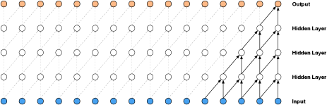
Fig. 3: A pictorial representation of regular causal convolutions (figure replicated from Oord et al. [42]). Observe how the receptive field size increases linearly with the number of layers.

Fig. 4: A pictorial representation of dilated causal convolutions (figure replicated from Oord et al. [42]). Each layer doubles the dilation rate, starting from a dilation rate of 1, or normal causal convolutions. This results in an exponential increase in receptive field size compared to a linear increase with normal causal convolutions (see Figure 3).

With traditional convolutional operations, filters in each layer convolve with their input volumes to produce feature maps. Specifically, in ResNet-18, each filter has a small receptive field of size 3, meaning that it can only operate on inputs that are at most two apart from each other. Of course, higher-up layers operate on lower layers, compounding receptive field, but this still results in each layer having a receptive field that only grows linearly with the number of layers, as shown in Figure 3.

While a linear increase may be sufficient in image classification problems where the inputs typically contain smaller and more locally-defined features, packet sequences often have a much more long-term and intertwined structure. For instance, consider classifying a human face. Typically, the classifier would first detect smaller facial features such as eyes, mouth, and ears, and combine these features at a higher level to detect a face. The smaller features happen within local spatial regions and can thus be detected with linear receptive field increases. In contrast, when a user contacts a server to download data, that might cause a cascading ripple effect wherein several hundred streams of packets are sent before that one transmission is completed. This insight about the long-term and temporally-related nature of packet sequences motivates the following exploration of dilated convolutions.

Strictly speaking, a larger increase in receptive field size could be achieved through uniformly larger filters. However, in practice this results in far more weight parameters and thus increases training time and memory. RNNs such as Long Short-term Memory Networks [20] have also traditionally provided support for temporal data, but we found that the length of our packet sequence proved to be prohibitively long for current RNN optimization techniques.

Instead, we build long-term temporal understanding into our CNN model by utilizing dilated convolutions [47, 42], convolutions that skip inputs at a certain dilation rate. Intuitively, instead of taking a fine-grain view of a small input region, dilated convolutions allow the network to take a coarse, wide view of the network, as shown in Figure 4. Since the actual filter used in dilated convolutions is still the same as in regular convolutions, the number of parameters and training cost do not increase.

Our model doubles dilation rates in every convolutional layer until hitting an upper-bound of dilation 8, upon which it cycles back to dilation 1 (i.e., dilation rates are {1, 2, 4, 8, 1, 2, 4, 8, …}). Instead of a linear increase in receptive field size, this results in an exponential increase, albeit for a small number of steps, as shown in Figure 4. This technique has shown to be effective in Image Segmentation [47], Audio Synthesis [42], and Computational Biology [15].

Finally, as did Oord et al. in their WaveNet model [42], we also combine dilated convolutions with causal convolutions, which simply restrict every neuron to only look at neurons from previous timesteps. This helps Var-CNN better map the inherent temporal dependencies of packet sequences. For instance, we found that using dilated causal convolutions results in an increase in accuracy from 94% to 96% in a closed-world of 100 monitored sites and 90 monitored instances.

4.4 Cumulative statistical features

In addition to automatically extracting features from the raw data with ResNet-18, we also provide seven basic cumulative features to the model. These features include the total number of packets, the total number of incoming packets, the total number of outgoing packets, the ratio of incoming to total packets, the ratio of outgoing to total packets, the total transmission time, and the average number of seconds to send each packet.

Based on our experiments, a fully-connected layer with cumulative features as input achieves only 35% accuracy in a small closed-world (100 sites, 90 instances). Due to the low accuracy, if we combined the metadata input and ResNet-18 post-training by averaging their softmax outputs, it would reduce the overall accuracy (see Appendix A for further details). For example, in a small closed-world, adding metadata post-training results in an accuracy decrease in the dilated causal ResNet-18 from 96% to 95%. Instead, we combine the fully-connected metadata layer with the ResNet-18 during training by concatenating their outputs, as shown in Figure 5. Finally, after concatenation, the combined output is sent through another fully-connected layer with Dropout regularization [39] before going to the final softmax output. Intuitively, this in-training ensemble scheme allows for the ResNet-18 AFE model to automatically learn how to supplement its strong predictions with the weak predictions from cumulative manually extracted features. In practice, for a small closed-world, this results in an accuracy increase from 96% to 97% for the dilated causal ResNet-18. We note that while improvements seem marginal in this small closed-world setting, they are amplified in more complex settings where accuracies are lower (e.g., see §5.2.1).

Var-CNN is the first WF attack to supplement automatically extracted ResNet-18 features with cumulative manually extracted features. Because of this, we consider Var-CNN a semi-automated feature extraction model.

4.5 Inter-packet timing

To the best of our knowledge, low-level timing data (i.e., the timestep at which a packet was sent or a close derivative of it) has never been effectively used in prior art. For instance, Bissias et al. [4] used inter-packet timings in an early WF attack. However, compared to prior art at the time using different features, their attack did not perform as well [16]. More recently, Wang et al. [43] used total transmission time as one of their features, and Hayes et al. [16] did a feature importance study using inter-packet times. As shown by Hayes et al., however, these low-level time features ranked 40^th–70^th in feature importance, making them essentially useless for classification.

Rather than dismiss packet timing, we applied the dilated ResNet-18 without metadata (§4.3) and observed some interesting outcomes. Without changing any parameters and only switching direction information with inter-packet times, the ResNet-18 with packet timing data achieved accuracy nearly comparable to that of a ResNet-18 with direction data (96% to 93%, respectively, in a closed-world with 100 sites and 90 instances). Moreover, by combining it with the basic cumulative features described in §4.4, we were able to achieve a 1% accuracy improvement from 93% to 94% that is on par with what we observed for the direction ResNet.

In contrast to prior work with manually extracted timing features, the high accuracy of ResNet-18 with timing data indicates that packet timing does leak a significant amount of information. Apart from the suggested privacy leakage, Var-CNN with timing data highlights one of the key benefits of AFE over manual feature extraction: performance under domain shifts. Though no prior features have been discovered to effectively use timing data, the ResNet-18 is both general enough to take in any sequence-like input and powerful enough (with a strong ResNet architecture and our augmentations) to perform well with these inputs.

As we will see in §5.2.1, ResNet-18 with time data is not as accurate as ResNet-18 with direction data. However, we describe a way to combine the two in §4.6 to improve the performance of the final classifier.

4.6 Ensemble of timing and direction

Fig. 5: A graphical representation of our ensemble model with just three output classes, 2 monitored sites and the unmonitored (UM) class. Each of the direction and time models is trained separately in conjunction with metadata inputs. Finally, the two models’ softmax layers are averaged post-training. TH signifies a minimum confidence threshold of a certain value over the averaged softmax outputs. The internals of the dilated causal ResNet-18 are shown in Figure 2.

In §4.4, we combined the ResNet-18 with cumulative features in-training since the fully-connected layer with cumulative features alone was far less accurate than the ResNet. In contrast, both the time and direction ResNets with cumulative features are highly accurate (as we will see in §5.2.1). Consequently, we found that their accuracy actually dropped (from 97% for the direction model to 95% for the direction and time model in a small closed-world) when combining them during training. This is most likely due to overfitting caused by training on essentially $2\times$ the number of parameters, which makes the underlying optimization problem much more difficult (see Appendix A for further details).

Instead, to effectively combine direction and timing, we take the arithmetic mean of their softmax outputs after training each model separately. This has the advantage of making each individual optimization procedure no more parameter-intensive than the original, single-model optimizations. We experimented with other averaging schemes (see Appendix A for further details) and found that even the optimal weighted average (i.e., the highest performing average over the test set) always used each model equally, plus or minus a small $\epsilon$. Since a simple arithmetic mean is near-optimal, the final Var-CNN model performs this over the outputs of the ResNet-18 direction and time models with cumulative features, as shown in Figure 5. In §5.2.1, we provide empirical results that show how the averaging scheme described here provides consistent improvements over the accuracy of each individual model.

4.7 Confidence threshold

As the final step of our attack, we apply a post-training threshold on the softmax probability output of the network (indicated by the “TH” block in Figure 5). If the output class probability is less than this threshold, we change the predicted class to the unmonitored class. Intuitively, this can be explained as defining a certain minimum bound on model certainty before classifying a sample. If a model is not certain about its classification as a monitored website, we assume that the testing input was really an unmonitored website that only partially matched a monitored site, and we classify it as unmonitored.

The threshold constraint also allows for direct control over TPR and FPR trade-off. Prior manual feature extraction work achieved this using methods such as classify-verify [24], using an additional classifier on top of features outputted from a primary classifier [16], and changing the number of nearest neighbors in $k$-NN [43, 16]. However, in the case of using a different model to perform final classification, this results in increased computational time due to training multiple models and decreased accuracy due to information loss between the feature extractor and classifier. Additional schemes such as classify-verify and adjusting the number of nearest neighbors require re-training to adjust trade-offs.

In contrast, Var-CNN allows us to easily adjust thresholds post-training. With a threshold of 0, this is the equivalent of not applying any model constraint. When the threshold is 1, we restrict the network to only classify websites as monitored if it is 100% certain, decreasing the number of true positives and false positives. We discuss empirical results for the TPR-FPR trade-off in §5.2.2. We further note that since confidence thresholds result from having a final discrete softmax probability output, both Rimmer et al.’s [36] and Sirinam et al.’s [38] deep learning-based attacks have them.

5 Var-CNN evaluation

In this section, we describe our experimental setup and evaluate Var-CNN.

5.1 Experimental setup

5.1.1 Dataset

Unfortunately, Sirinam et al.’s dataset was not available at the time of writing. Instead, we evaluate our attack on the Rimmer et al. dataset [36], which was publicly available. However, since the public dataset does not have enough information to extract inter-packet time and metadata, we processed their unfiltered dataset, which we obtained upon request.

This dataset has a total of 900 monitored sites each with 2,500 traces. For open-world, there are a total of 500,000 additional unmonitored sites, each with only 1 trace. Both the monitored and unmonitored pages were compiled from the Alexa list of most popular sites [1], and with over 2.75 million total traces, it is one of the largest and most up-to-date WF datasets in existence.

For each of our three different models, we feed in a different set of features representing a given trace. The direction ResNet-18 takes in a set of 1’s and -1’s that represents the direction of each packet. The numbers 1 and -1 respectively denote outgoing packets (which travel toward the web server) and incoming packets (which travel toward the client). The time ResNet-18 takes in a sequence of floats that represent the time delay between when a current packet and the previous packet is sent. The metadata model takes in seven floats (for the seven cumulative statistical features described in §4.4). Since CNNs only take in a fixed-length input, we pad and truncate each set of inputs to the direction and time models to the first 5,000 values. This is consistent with prior work [36, 38] and strikes a balance between the computational overhead of larger sequences and the information loss of smaller sequences.

5.1.2 Training/Validation/Test Split

In all our experiments, we use the exact same training, validation, and test data for both Var-CNN and DF [38]. Although manually extracted attacks used cross-validation on smaller datasets [43, 34, 16], this is computationally infeasible on our larger dataset. Instead, we follow the best practices of the deep learning community and the practices of Sirinam et al. [38] and split data into a training, validation, and test set. No random data split favors any model because we use the same split for both models.

In all our settings, we used a random 10% of all monitored traces (i.e., 10% of the traces from each website) for testing and a random 5% of the remaining 90% of all monitored traces (regardless of website) for validation. While the number of unmonitored training and testing sites differs with every setting, we use a random 5% of all unmonitored training sites for validation. There is no overlap between data used for training, validation, and testing. In addition, note that we use the validation set to time learning rate decays and stop model training (see Appendix A.2 for further details).

5.1.3 Model Implementation

To implement Var-CNN, we use Keras [8] with the TensorFlow [2] backend. As Sirinam et al.’s code was not available at the time of writing, we reimplemented their model with their guidance in the same Keras and Tensorflow environment they used [38]. Given that neural networks train several times faster on GPUs due to data parallelism, we run our experiments on NVIDIA GTX 1080Ti workstations at our organization with 11 GB of GPU memory.

5.1.4 Hyperparameter Tuning

To determine hyperparameters for Var-CNN, we systematically go through each hyperparameter, sweeping a certain range of values while keeping all other hyperparameters constant. After finding a well-performing value, we fix it and then test other hyperparameters. As mentioned in §4, we measure performance using accuracy on the test set for a small closed-world with 100 sites and 90 instances. After selecting hyperparameters (e.g., architecture, regularization, and starting learning rate) on this small closed-world, we fix them for all subsequent open- and closed-world evaluations in §5.2. Our main reason for selecting hyperparameters once using a small dataset was to increase the speed of our research, and we reported closed-world accuracies in §4 simply to provide a metric for the performance differences of various Var-CNN architectural choices, not as a point of comparison against other attacks.

For further details on the specific parameters we used and for additional information on model design choices that worked and did not work, see Appendix A. Note that our parameter search was by no means extensive, especially for the ResNet-18 with packet timing data. It is entirely possible that different Var-CNN configurations perform differently on direction data versus time data, but we made a simplifying assumption to use the same configuration. In addition, this showcases Var-CNN’s input generality and high performance under domain changes.

5.2 Experimental results

In this section, we discuss our various experiments and their implications.

5.2.1 Comparison of Var-CNN variants

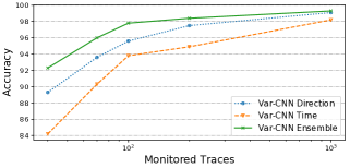
Fig. 6: Closed-world accuracies of Var-CNN direction, Var-CNN time, and Var-CNN ensemble. Experiments are run with 100 monitored sites and a varying number of traces per site. Accuracies are in % and the x-axis is logarithmically scaled.

We first compare the three different configurations of Var-CNN: direction, time, and ensemble.

Figure 6 shows accuracies for these three configurations as we change the number of monitored traces in a closed-world setting. First, we observe that while the time model always gets less accuracy than the direction model, both are still highly comparable. For instance, with 1000 traces, the accuracy difference is only 0.9%, meaning both models are highly accurate. While prior art was unable to effectively use low-level timing data (§4.5), we show that AFE can take advantage of this information. Var-CNN effectively classifies websites solely based on timing data without any major modifications.

Second, the ensemble model combining direction and time always has higher accuracy than either of its constituents. While this may seem obvious at first—two models must always be better than one—it suggests that the two models seem to complement each other’s predictions. If both were highly confident on the exact same predictions, then the ensemble created by averaging their outputs would not improve. Instead, it appears that there are some situations where one model is more confident than the other, and vice-versa. These situations average out such that the ensemble model produces better overall predictions than either of its constituents.

5.2.2 TPR-FPR trade-off

Fig. 7: The TPR and FPR trade-off for an open-world setting with 100 monitored sites, 1,500 monitored traces, 150,000 unmonitored training sites, and 100,000 unmonitored testing sites. Multi-TPR and FPR are in % and the upper left corner is the best. Data points farther up and to the right use lower confidence thresholds.

As discussed in §4.7, Var-CNN allows TPR-FPR trade-off by changing the confidence threshold post-training. Using a higher confidence threshold, the attacker can lower FPR by assuming that traces predicted as a monitored site with low confidence are actually false positives. This greedy scheme naturally causes true negatives, i.e., monitored traces classified as unmonitored due to their relative dissimilarity to other monitored traces. A similar technique can also be applied to DF, and in Figure 7, we plot this trade-off for both attacks in our largest open-world setting tested.

As can be seen, both TPR and FPR decrease as the confidence threshold increases and the graph goes to the bottom left. For instance, with a threshold of 0.5, Var-CNN has a 98.01% Multi-TPR and a 0.36% FPR. As the threshold increases to 0.9, Var-CNN’s TPR goes down to 93.68% but its FPR also goes down to 0.10%. With 100,000 unmonitored testing sites, this is a reduction of 260 false positives to only 100 false positives compared to the initial 360 false positives.

Another interesting trend is the difference between Var-CNN and DF FPR for the same Multi-TPR. When both attacks use a threshold of 0, for nearly the same TPR, DF has an FPR of 3.28%, which is over $7\times$ that of Var-CNN at 0.45%. In addition, this difference gets larger for increasing Multi-TPR, indicating that Var-CNN has significant FPR benefits when the attacker needs to maximize TPR.

5.2.3 Closed-world performance

Fig. 8: Var-CNN and DF closed-world accuracy as a function of the number of monitored traces for each of 100 monitored sites. Results are in % and the x-axis is logarithmically scaled.

Fig. 9: Var-CNN and DF closed-world accuracies for larger settings with 2500 monitored traces and a varying number of monitored sites. Results are in %.

We now consider closed-world experiments with varying amounts of training data. Figure 8 shows Var-CNN and Deep Fingerprinting accuracy as the number of traces increases for each of 100 monitored sites. First, observe Var-CNN’s high accuracy even in settings with relatively small numbers of traces. For instance, with 100 traces, Var-CNN achieves 97.8% accuracy while DF achieves 93.6% accuracy. It would take $5\times$ as much training data (i.e., 500 traces) for DF to achieve a comparable accuracy of 98.1%.

In general, this accuracy difference does not stay stagnant over time. Rather, Var-CNN’s accuracy improvements tend to increase as the number of traces decreases. For example, at 2000 traces, our largest amount tested, there is a 0.39% accuracy gap. This increases to 0.8% with 500 traces, 2.1% with 200 traces, 4.2% with 100 traces, 6.8% with 50 traces, and 11.75% with 40 traces.

As shown in Figure 9, Var-CNN also has large accuracy increases in closed-world settings with many sites and a large number of traces per site. For instance, with just 100 sites and 2500 traces, both attacks achieve near comparable accuracy with a difference of 0.3%. However, as the number of monitored sites increases with no additional traces, the gap between Var-CNN and DF accuracy also increases to 0.6% with 200 sites (99.5% compared to 98.9%), 1.8% with 500 sites (99.2% compared to 97.4%), and 2.3% with 900 sites (98.8% compared to 96.5%). §6.2 provides a unifying explanation for the increasing accuracy gap phenomenon in both low-data and high-data scenarios.

5.2.4 Open-world performance

(a)

(b)

(c)

Fig. 10: Var-CNN and DF’s (a) Two-TPR, (b) Multi-TPR, and (c) FPR as a function of the attacker’s data collection capabilities. Here, we use 100 monitored sites and 100,000 unmonitored testing sites. For each setting, we use monitored traces and unmonitored training sites in a 1:100 ratio. We choose a confidence threshold of 0.5 for Var-CNN and 0.8 for DF. Results are in % and the x-axis is logarithmically scaled.

We now evaluate Var-CNN and DF in the open-world setting. Here, both the number of monitored traces per monitored site and the number of unmonitored training sites affect TPR and FPR. Generally, more monitored traces leads to a better knowledge of the monitored class and a higher TPR, while more unmonitored training sites biases the attack model towards correctly separating monitored from unmonitored, reducing FPR. Of course, these trends are not exact, as strictly increasing the number of unmonitored training sites also introduces noise in monitored classification, slightly reducing TPR.

We assume that the adversary can collect enough of both types of traces to balance out possible negating effects. Specifically, we quantify the attacker’s data collection capabilities by using a varying number of monitored traces and unmonitored training sites in a 1:100 ratio. We now study how Var-CNN and DF perform under an adversary with varying data collection capabilities. For all our experiments, we picked confidence thresholds such that both attacks had a good balance of TPR and FPR and used these across all data settings.

In large open-worlds where the attacker must separate perhaps billions of unmonitored sites from monitored, false positives are often the limiting factor [34]. For example, with a million unmonitored traces, an FPR of even 0.1% results in 1,000 false positives. Observe in Figures 10(a), 10(b), and 10(c) that for both Var-CNN and DF, Two-TPR increases, Multi-TPR increases, and FPR decreases as the adversary’s data collection capabilities increase. Assuming the probability of an unmonitored site falsely classified as a monitored site stays the same for an arbitrarily sized open-world, an adversary can thus reduce false positives and increase true positives by scaling the amount of training data. Furthermore, Var-CNN performs better than DF in these high-data settings (i.e., settings with a large number of traces per trial), with over $4\times$ lower FPR (1.47% to 0.36%), over 1% better Two-TPR (96.45% to 98.07%), and over 1% better Multi-TPR (96.39% to 98.01%).

While Var-CNN outperforms DF in high-data settings, its accuracy improvements are especially useful as the amount of training data decreases. In Figures 10(a), 10(b), and 10(c), we observe that the gap between Var-CNN and DF generally tends to increase as the amount of data decreases. For instance, the Multi-TPR gap is 2.22% with 1000 traces, 7.13% with 80 traces, and 13% with 60 traces. At these same scales, the FPR gap is 1.11%, 2.21%, and 3.12%, respectively, and the Two-TPR gap is 2.13%, 6.62%, and 11.34%, respectively. This indicates that an attacker with fewer capabilities for collecting large amounts of training data has a better probability of both fingerprinting a user while not falsely identifying them with Var-CNN. §6.2 relates this phenomenon to those observed in the closed-world setting and provides a possible unifying explanation.

5.2.5 Comparison against other attacks in the presence of WF defenses

Table 1: Open-world Multi-TPR and FPR for Var-CNN evaluated against three other state-of-the-art attacks. Evaluations are done in both natural settings (None) and WF defense settings against a constant-flow WF defense (Tamaraw) and a WF defense based on adaptive padding (WTF-PAD). We use 100 monitored sites, 100 monitored traces, 90000 unmonitored training sites, and 10000 unmonitored testing sites for this evaluation and simulate the attacks and defenses with the original code from each author. Note that Var-CNN gets higher Multi-TPR and lower FPR than any other attack, even in settings with WF defenses. Furthermore, note that Multi-TPR and FPR for Tamaraw is zero across nearly all attacks since the strong defense causes all attacks to classify every trace as unmonitored. The only exception is with $k$-FP, which we further explain in §5.2.5.

Defenses	Overhead		Var-CNN		DF [38]		$k$-FP [16]		CUMUL [34]
	Bandwidth	Latency	Multi-TPR	FPR	Multi-TPR	FPR	Multi-TPR	FPR	Multi-TPR	FPR
[]None	0%	0%	89.2%	1.1%	88.4%	8.6%	70.4%	9.1%	85.6%	10.2%
Tamaraw [5]	63%	51%	0.0%	0.0%	0.0%	0.0%	4.1%	54.3%	0.0%	0.0%
WTF-PAD [25]	27%	0%	88.8%	0.7%	86.2%	5.4%	71.1%	9.5%	78.1%	12.6%

While DF outperformed prior art on Sirinam et al.’s dataset [38], these attacks have never been simultaneously tested on the Rimmer dataset [36]. In this experiment, we evaluate Var-CNN and DF against prior art in settings with and without WF defenses. Note that here we exclude $k$-NN [43] from our evaluation since it has been shown by several researchers to be less accurate than both $k$-FP and CUMUL [16, 34, 36, 38].

First, we assess our original assumption that DF is the current state-of-the-art WF attack. The first row in Table 1 shows Multi-TPR and FPR for all attacks in a medium-sized open-world with no WF defense. Since DF has a higher Multi-TPR and lower FPR than all prior art, it is still the current state-of-the-art attack, even on the Rimmer dataset [36]. As noted by Sirinam et al. [38], it also performs comparably or slightly better than all prior art in WF defenses settings against Tamaraw and WTF-PAD.

Having shown DF to be the best prior-art attack in settings with and without WF defenses, we now assess Var-CNN’s performance relative to DF. In the undefended scenario, Var-CNN (with a confidence threshold of 0.5) attains similar Multi-TPR to DF (with a confidence threshold of 0.7), 89.2% compared to 88.4%. However, it has a nearly $8\times$ lower FPR, going from 8.6% to 1.1%. Thus, compared to Var-CNN, DF would incorrectly classify several more unmonitored websites as being monitored, thereby falsely identifying users.

In the WF defense setting against Tamaraw and WTF-PAD, Var-CNN still retains significant improvements over DF and the rest of the prior-art. For example, with a Multi-TPR comparable to that of DF (88.8% compared to 86.2%, respectively), Var-CNN achieves a nearly $8\times$ reduction in FPR from 5.4% to 0.7%. Against other attacks such as $k$-FP and CUMUL, Var-CNN has even greater improvements in both Multi-TPR and FPR.

Finally, we note that after trying several configurations of Tamaraw, we were unable to get a configuration that yielded non-zero Multi-TPR and FPR for all attacks. While $k$-FP did manage to get a 4% Multi-TPR against Tamaraw, the resulting FPR of 54.3% is too high to make reliable predictions. Indeed, it appears that our Tamaraw configurations were so strong that they caused most attacks to classify every instance as being unmonitored, resulting in 0% TPR and 0% FPR. In contrast, WTF-PAD (at least under the configuration we tested) sacrifices too much security for low overheads. As noted by Sirinam et al. [38], it fails to protect against attacks like Var-CNN and DF, which achieve relatively high TPR and relatively low FPR.

6 Discussion

In this section, we discuss pertinent aspects of Var-CNN.

6.1 A note on runtimes

Note that with some experimental settings, both DF and Var-CNN could possibly achieve better accuracies if allowed to train for longer. However, this adds yet another parameter the attacker must optimize for and introduces additional training time overheads. We therefore made a simplifying assumption here to use the same stopping scheme for each model across all experiments (see Appendix A for more details).

One of the weaknesses of Var-CNN is that it takes a longer time on average to train than DF due to the more complex underlying model (ResNet-18), additional fully-connected layer for basic cumulative features, and time model. For example, for a closed-world with 100 monitored sites and 100 traces per site, it took approximately 25 minutes to train Var-CNN using one GPU while it took around 4 minutes to train DF. These runtimes scale roughly proportionally with the amount of training data used.

While Var-CNN does cause increased runtimes, we believe they are offset by its much improved performance in all settings tested. For example, for DF to reach a comparable accuracy to Var-CNN in a closed-world with 100 sites and 100 traces, it would need approximately $5\times$ the number of traces (§5.2.3). Moreover, we can parallelize the training procedure to decrease runtimes. Since Var-CNN direction and Var-CNN time are independent models ensembled after training, they can be trained separately on two GPUs. In addition, recent work in Deep Learning research has shown that models can be massively parallelized by using larger batch sizes, special learning rate schemes, and more GPUs. A prime example of this is Goyal et al. [14], who trained a ResNet-50 on a very large image classification dataset in just one hour. Previously, it would have taken several days to train on a single GPU.

6.2 Why does Var-CNN work in low-data settings?

As noted in §5.2.3 and §5.2.4, Var-CNN’s accuracy improvements over DF increase in the following scenarios:

1. A fixed number of monitored sites and a decreasing number of monitored traces in the closed-world.

2. A fixed number of monitored traces and an increasing number of monitored sites in the closed-world.

3. A decreasing number of monitored traces and unmonitored training sites in the open-world.

In this section, we provide a possible general explanation for these trends and relate them to the model techniques used in Var-CNN.

For the following discussion, consider neural network optimization as finding a good hypothesis (i.e., one that achieves low training and generalization errors) among the overall hypothesis space. All of the above settings make the hypothesis space more vast and ambiguous to traverse. For instance, decreasing the number of monitored traces and unmonitored train sites (i.e., reducing the training data available to the classifier) provides less information for the optimizer to find a good hypothesis with low generalization error. On the other hand, increasing the number of monitored sites as in the second scenario expands the overall size of the hypothesis space with no additional optimization help from more monitored traces. As the hypothesis space changes, a modern convolutional neural network with enough weight parameters would still likely achieve good training accuracy, as shown by Zhang et al. [48]. However, as the optimization landscape is more vast and ambiguous to traverse, it would have an increasingly difficult time finding hypotheses that don’t overfit to the training data (i.e., that have low generalization error).

In contrast, one of the key benefits of ensembles, as noted by seminal work [10], is statistical. When the hypothesis space becomes unclear as with the above scenarios, ensembles help filter out bad hypotheses that overfit to the training data, making the overall model have better generalization capabilities. Given that Var-CNN is composed of two types of ensembles, one with an in-training combination of a dilated causal ResNet-18 and cumulative features and the other with a post-training ensemble of direction and timing models, we suspect that these ensembles enable Var-CNN to perform especially well when the optimization landscape gets more complex to navigate. Empirically, this was also observed in §5.2.1, where the gap between the ensemble model and the best performing constituent increases as the number of monitored traces decreases.

7 Future work

Although Var-CNN outperforms prior WF attacks in every setting tested, especially with small amounts of training data, there are still many directions where it could improve. In this section, we discuss limitations of our work and possible avenues for future work.

More powerful baseline models. Since deep learning is a rapidly accelerating field [28], applications of new model architecture breakthroughs could lead to better results. For instance, here, we used the ResNet architecture as our baseline CNN since it is currently the most widely used state-of-the-art Image Classification CNN. There are other Image Classification models such as larger variants of ResNets or DenseNets [21] that could give better results. In our preliminary tests with these architectures, however, we did not see significant-enough accuracy improvements to justify their increased computational costs.

In addition, recent work on Synthetic Gradients [23] could lead to RNNs with the ability to train on much longer inputs (e.g., the packet sequences used in this work). Since RNNs were specifically made for temporal sequences, this model might understand long-term packet interactions better than dilated causal convolutions.

Regardless of the architecture choice, we would like to note that nearly all of the packet sequence classification insights used in this paper are architecture-independent and can thus be applied to most future deep learning attacks. For instance, dilated causal convolutions work with any CNN architecture and ensembles with cumulative features and timing data work with nearly all neural network models.

Data augmentation. A common technique in Computer Vision research is to artificially expand the training data size by using data augmentation—cropping, rotating, flipping, shifting, and rescaling the image. This technique works in Computer Vision because the artificial data is often similar-enough to real-world data that it is useful to the model. Similar techniques for packet sequences, such as shifting them a random number of packets one way or the other, could be used to achieve even better low-data performance.

User-sourced datasets. As described in §2.2, there are two main types of assumptions, replicability and applicability. Both of these assumptions could be tested in a real-world user trial study. Here, an adversary would draft a number of real-world Tor users and monitor their packet sequences, sites visited (including background traffic), and metadata settings (Tor versions, circuit latencies, etc.). This would enable them to know how strong the WF assumptions are in the real-world.

Adversarial machine learning. Regular WF defenses such as recent work by Lu et al. [31] and Wang et al. [46] degrade accuracy by blocking information leakage from sources such as inter-packet timing, packet sequence length, and burst patterns. However, more precise WF defenses could exist within the context of adversarial attacks on machine learning models [13]. Assuming the WF defender has some knowledge of the WF attacker model, she might be able to craft specialized perturbations to reduce the model’s classification ability while introducing less overhead than more traditional WF defenses.

One challenging problem here is defining a useful constraint for adversarial attacks. Most work in adversarial machine learning has focused on image classification, where $\ell_{p}$ norms constrain the total amount of pixel-level perturbation allowed for an image. With packet sequences, however, it is much harder to change individual inputs as they must obey temporal orderings. For example, an outgoing packet cannot be changed to incoming if that information is necessary in the future. The same argument applies to changing the timestamp of a packet. Thus, creating a specialized constraint for the set of all allowable perturbations will most likely be the focus of future work.

Finally, as with all attack-defense paradigms, while adversarial machine learning WF defenses might be able to initially defeat WF attacks, new WF attacks could be trained to become robust against these defenses. For instance, recent work by Mądry et al. has shown that by viewing adversarial machine learning within the context of convex optimization, one can train a model that is robust to adversarial input [33]. This would allow for a WF attack to be resistant to adversarial WF defense perturbations.

Code release. To support future work, we have made our code, including our re-implementation of DF, publicly available at https://github.com/sanjit-bhat/Var-CNN. Please refer to Rimmer et al.’s paper [36] for instructions on downloading their dataset.

8 Conclusion

In this work, we present Var-CNN, a novel website fingerprinting attack that combines a strong baseline ResNet CNN model with several powerful insights for packet sequence classification: dilated causal convolutions, automatically extracted direction and timing features, and manually extracted cumulative features. In open-world settings with large amounts of data, Var-CNN achieves over 1% better TPR and $4\times$ lower FPR than prior-art. In addition, Var-CNN’s improvements are especially relevant in low-data scenarios, where deep learning models typically suffer. Here, it reduces prior-art FPR by 3.12% while increasing TPR by 13%.

Overall, Var-CNN’s model insights, which can be applied to most future neural network models, allow it to need less training data than prior art. This lowers the likelihood of data staleness performance issues and allows a weaker attacker with fewer data collection resources to successfully perform a powerful WF attack.

9 Acknowledgements

This work was done as part of the MIT PRIMES program while Sanjit Bhat and David Lu were students at Acton-Boxborough Regional High School. The authors were partially supported by National Science Foundation grant No. 1813087. The authors would like to thank Dimitris Tsipras and the Mądry Lab at MIT for providing some of the compute resources used to run these experiments.

Appendix A Var-CNN model design

To come up with the final Var-CNN model, we performed several different experiments testing various aspects of the model design. Here, we mention a few important results. For full parameter choices, please refer to our code.

A.1 Ensemble schemes

One of our main problems was deciding how to most effectively combine the direction, time, and metadata models. First, note that each model yielded varying standalone performance. For instance, in a closed-world with 100 sites and 90 monitored traces, both the direction and time models achieved above 90% accuracy while the metadata model consistently got 35% accuracy. If we just averaged all three models post-training, this caused an accuracy decrease since the metadata model was significantly worse than the other two. This finding led us to use metadata during training rather than after. In our tests, we noticed that adding metadata to both the direction and time ResNets acted as a stabilizer, reducing stochasticity and improving final accuracy. Intuitively, the overall model learned when to use the automatically extracted ResNet features over the manually extracted cumulative features, and vice-versa, balancing each source of information.

Now that we knew to combine the ResNet with the cumulative features in-training, one remaining question was how to combine the direction and timing information. In early experiments, we tried to use in-training weight-sharing techniques. While this certainly did not double the number of model parameters, it resulted in an accuracy drop compared to the individual direction and timing models. This was likely due to the dissimilarity between direction and timing inputs (e.g., on a meta-level, the former is sampled from a discrete distribution while the latter from a continuous distribution). As a result, features learned from direction inputs were markedly different from those learned from timing inputs, and the shared model struggled to find a set of shared weights.

Unfortunately, the alternative to weight sharing—an in-training combination of two separate direction and timing models—often led to reduced accuracy as the fundamental optimization problem got much harder with twice the number of parameters. Instead, we ensembled these models post-training by combining their softmax outputs. In our experiments, we compared various schemes for combining, such as using the validation set to find a weighted average and doing simple averaging, against a simple sweep to find the optimal weight. In most cases, our results indicated that the first method was overfitting the validation set, whereas a simple average usually achieved near-optimal accuracy. Therefore, for the final Var-CNN model we performed a simple average over the softmax outputs of the direction and time models trained jointly with metadata, as shown in Figure 5.

A.2 Learning rate decay and early stopping

Rather than having a fixed learning rate drop-off scheme with a fixed number of epochs, we found it much more effective to decide these based on validation set performance. Specifically, we started training with a learning rate of 0.001, the default value for the Adam optimizer [26], and allowed the network to train for 5 epochs without improving validation accuracy before we reduced learning rate by a factor of $\sqrt{0.1}$ (i.e., $new\textunderscore lr=\sqrt{0.1}*old\textunderscore lr$). The minimum possible learning rate was 0.00001, and we stopped training after not improving validation accuracy for 10 epochs, twice the number used for learning rate decay. We saved the best performing model on the validation set and reloaded this model to perform final classification on the test set.

Two parameters we experimented with here were the initial learning rate and the base patience used for learning rate decay. From our experiments, reducing learning rate from the default resulted in higher local minima in the loss landscape, while increasing learning rate did not improve model accuracy. Increasing base patience sometimes allowed for slightly better accuracy, but it also significantly increased the average number of epochs for training. With a base patience of 5, both the direction and time models used between 30–50 epochs across all experimental settings.

A.3 Dropout and $\ell_{2}$ decay

With both the direction and time models, training accuracy reached around 99.99% by the end of training, indicating that the model may have overfit to the training data. To curb this, we tried various mechanisms, such as introducing Dropout [39] and $\ell_{2}$ decay to the ResNet model and the final fully-connected layer after concatenating the ResNet and metadata models. We observed that $\ell_{2}$ decay did not manage to reduce overfitting on the ResNet. However, using a Dropout rate of 0.5 on the final fully-connected layer did reduce overfitting to some extent, decreasing the generalization error.

References

- [1] The Top 500 Sites on the Web. https://www.alexa.com/topsites, 2017.
- [2] Martín Abadi, Ashish Agarwal, Paul Barham, Eugene Brevdo, Zhifeng Chen, Craig Citro, Gregory S. Corrado, Andy Davis, Jeffrey Dean, Matthieu Devin, Sanjay Ghemawat, Ian J. Goodfellow, Andrew Harp, Geoffrey Irving, Michael Isard, Yangqing Jia, Rafal Józefowicz, Lukasz Kaiser, Manjunath Kudlur, Josh Levenberg, Dan Mané, Rajat Monga, Sherry Moore, Derek Gordon Murray, Chris Olah, Mike Schuster, Jonathon Shlens, Benoit Steiner, Ilya Sutskever, Kunal Talwar, Paul A. Tucker, Vincent Vanhoucke, Vijay Vasudevan, Fernanda B. Viégas, Oriol Vinyals, Pete Warden, Martin Wattenberg, Martin Wicke, Yuan Yu, and Xiaoqiang Zheng. TensorFlow: Large-Scale Machine Learning on Heterogeneous Systems. arXiv preprint arXiv:1603.04467, 2015.
- [3] Kota Abe and Shigeki Goto. Fingerprinting Attack on Tor Anonymity using Deep Learning. In Proceedings of the Asia-Pacific Advanced Network Research Workshop, volume 42, pages 15–20, 2016.
- [4] George D. Bissias, Marc Liberatore, David Jensen, and Brian N. Levine. Privacy Vulnerabilities in Encrypted HTTP Streams. Privacy Enhancing Technologies, pages 1–11, 2006.
- [5] Xiang Cai, Rishab Nithyanand, Tao Wang, Rob Johnson, and Ian Goldberg. A Systematic Approach to Developing and Evaluating Website Fingerprinting Defenses. In Proceedings of the ACM Conference on Computer and Communications Security, pages 227–238, 2014.
- [6] Xiang Cai, Xin C. Zhang, Brijesh Joshi, and Rob Johnson. Touching from a Distance: Website Fingerprinting Attacks and Defenses. In Proceedings of the ACM Conference on Computer and Communications Security, pages 605–616, 2012.
- [7] Heyning Cheng and Ron Avnur. Traffic Analysis of SSL Encrypted Web Browsing. https://pdfs.semanticscholar.org/1a98/7c4fe65fa347a863dece665955ee7e01791b.pdf, 1998.
- [8] François Chollet et al. Keras. https://keras.io, 2015.
- [9] Tor Developers. Tor metrics portal. https://metrics.torproject.org, 2018.
- [10] Thomas G. Dietterich. Ensemble Methods in Machine Learning. In Proceedings of the International Workshop on Multiple Classifier Systems, 2000.
- [11] Roger Dingledine, Nick Mathewson, and Paul Syverson. Tor: The Second-Generation Onion Router. In Proceedings of the 13th USENIX Security Symposium, pages 303–320, 2004.
- [12] Kevin P. Dyer, Scott E. Coull, Thomas Ristenpart, and Thomas Shrimpton. Peek-a-Boo, I Still See You: Why Efficient Traffic Analysis Countermeasures Fail. In Proceedings of the IEEE Symposium on Security and Privacy, pages 332–346, 2012.
- [13] Ian J. Goodfellow, Jonathon Shlens, and Christian Szegedy. Explaining and Harnessing Adversarial Examples. In Proceedings of the International Conference on Learning Representations, 2015.
- [14] Priya Goyal, Piotr Dollár, Ross Girshick, Pieter Noordhuis, Lukasz Wesolowski, Aapo Kyrola, Andrew Tulloch, Yangqing Jia, and Kaiming He. Accurate, Large Minibatch SGD: Training ImageNet in 1 Hour. arXiv preprint arXiv:1706.02677, 2017.
- [15] Ankit Gupta and Alexander M. Rush. Dilated Convolutions for Modeling Long-Distance Genomic Dependencies. In Proceedings of the 34th International Conference on Machine Learning, Workshop on Computational Biology, 2017.
- [16] Jamie Hayes and George Danezis. -fingerprinting: A Robust Scalable Website Fingerprinting Technique. In Proceedings of the 25th USENIX Security Symposium, pages 1187–1203, 2016.
- [17] Kaiming He, Xiangyu Zhang, Shaoqing Ren, and Jian Sun. Deep Residual Learning for Image Recognition. arXiv preprint arXiv:1512.03385, 2015.
- [18] Dominik Herrmann, Rolf Wendolsky, and Hannes Federrath. Website Fingerprinting: Attacking Popular Privacy Enhancing Technologies with the Multinomial Naïve-Bayes Classifier. In Proceedings of the ACM Workshop on Cloud Computing Security, pages 31–42, 2009.
- [19] Andrew Hintz. Fingerprinting Websites Using Traffic Analysis. Privacy Enhancing Technologies, pages 171–178, 2003.
- [20] Sepp Hochreiter and Jürgen Schmidhuber. Long Short-Term Memory. Neural Computation, 9(8):1735–1780, 1997.
- [21] Gao Huang, Zhuang Liu, Laurens van der Maaten, and Kilian Q. Weinberger. Densely connected convolutional networks. In Proceedings of the IEEE Conference on Computer Vision and Pattern Recognition, 2017.
- [22] Sergey Ioffe and Christian Szegedy. Batch Normalization: Accelerating Deep Network Training by Reducing Internal Covariate Shift. In Proceedings of the 32nd International Conference on Machine Learning, 2015.
- [23] Max Jaderberg, Wojciech M. Czarnecki, Simon Osindero, Oriol Vinyals, Alex Graves, David Silver, and Koray Kavukcuoglu. Decoupled Neural Interfaces using Synthetic Gradients. In Proceedings of the 34th International Conference on Machine Learning, 2017.
- [24] Marc Juarez, Sadia Afroz, Gunes Acar, Claudia Diaz, and Rachel Greenstadt. A Critical Evaluation of Website Fingerprinting Attacks. In Proceedings of the ACM Conference on Computer and Communications Security, 2014.
- [25] Marc Juarez, Mohsen Imani, Mike Perry, Claudia Diaz, and Matthew Wright. Toward an Efficient Website Fingerprinting Defense. In Proceedings of the European Symposium on Research in Computer Security, pages 27–46, 2016.
- [26] Diederik P. Kingma and Jimmy Ba. Adam: A Method for Stochastic Optimization. In Proceedings of the 3rd International Conference on Learning Representations, 2015.
- [27] Alex Krizhevsky, Ilya Sutskever, and Geoffrey E. Hinton. ImageNet Classification with Deep Convolutional Neural Networks. In Proceedings of the Conference on Neural Information Processing Systems, pages 1097–1105, 2012.
- [28] Yann LeCun, Yoshua Bengio, and Geoffrey E. Hinton. Deep Learning. Nature, 521:436–444, 2015.
- [29] Yann LeCun, Leon Bottou, Yoshua Bengio, and Patrick Haffner. Gradient-Based Learning Applied to Document Recognition. Proceedings of the IEEE, 86(11):2278–2324, 1998.
- [30] Marc Liberatore and Brian N. Levine. Inferring the Source of Encrypted HTTP Connections. In Proceedings of the 13th ACM Conference on Computer and Communications Security, pages 255–263, 2006.
- [31] David Lu, Sanjit Bhat, Albert Kwon, and Srinivas Devadas. DynaFlow: An Efficient Website Fingerprinting Defense Based on Dynamically-Adjusting Flows. In Proceedings of the ACM Workshop on Privacy in the Electronic Society, 2018.
- [32] Liming Lu, Ee-Chien Chang, and Mun C. Chan. Website Fingerprinting and Identification Using Ordered Feature Sequences. In Proceedings of the European Symposium on Research in Computer Security, pages 199–214, 2010.
- [33] Aleksander Mądry, Aleksandar Makelov, Ludwig Schmidt, Dimitris Tsipras, and Adrian Vladu. Towards Deep Learning Models Resistant to Adversarial Attacks. In Proceedings of the International Conference on Learning Representations, 2018.
- [34] Andriy Panchenko, Fabian Lanze, Aandreas Zinnen, and Martin Henze. Website Fingerprinting at Internet Scale. In Proceedings of the 16th Network and Distributed System Security Symposium, 2016.
- [35] Andriy Panchenko, Lukas Niessen, Andreas Zinnen, and Thomas Engel. Website Fingerprinting in Onion Routing Based Anonymization Networks. In Proceedings of the ACM Workshop on Privacy in the Electronic Society, pages 103–114, 2011.
- [36] Vera Rimmer, Davy Preuveneers, Marc Juarez, Tom V. Goethem, and Wouter Joosen. Automated Feature Extraction for Website Fingerprinting through Deep Learning. In Proceedings of the Network and Distributed System Security Symposium, 2018.
- [37] Karen Simonyan and Andrew Zisserman. Very Deep Convolutional Networks for Large-Scale Image Recognition. arXiv preprint arXiv:1409.1556, 2014.
- [38] Payap Sirinam, Mohsen Imani, Marc Juarez, and Matthew Wright. Deep Fingerprinting: Undermining Website Fingerprinting Defenses with Deep Learning. In Proceedings of the ACM Conference on Computer and Communications Security, 2018.
- [39] Nitish Srivastava, Geoffrey H. Hinton, Alex Krizhevsky, Ilya Sutskever, and Ruslan Salakhutdinov. Dropout: A Simple Way to Prevent Neural Networks from Overfitting. Journal of Machine Learning Research, 15:1929–1958, 2014.
- [40] Qixiang Sun, Daniel R. Simon, Yi-Min Wang, Wilf Russell, Venkata N. Padmanabhan, and Lili Qiu. Statistical Identification of Encrypted Web Browsing Traffic. In Proceedings of the IEEE Symposium on Security and Privacy, pages 19–30, 2002.
- [41] Christian Szegedy, Sergey Ioffe, Vincent Vanhoucke, and Alex Alemi. Inception-v4, Inception-ResNet and the Impact of Residual Connections on Learning. arXiv preprint arXiv:1602.07261, 2016.
- [42] Aaron van den Oord, Sander Dieleman, Heiga Zen, Karen Simonyan, Oriol Vinyals, Alex Graves, Nal Kalchbrenner, Andrew Senior, and Koray Kavukcuoglu. WaveNet: A Generative Model for Raw Audio. arXiv preprint arXiv:1609.03499, 2016.
- [43] Tao Wang, Xiang Cai, Rob Johnson, and Ian Goldberg. Effective Attacks and Provable Defenses for Website Fingerprinting. In Proceedings of the 23rd USENIX Security Symposium, pages 143–157, 2014.
- [44] Tao Wang and Ian Goldberg. Improved Website Fingerprinting on Tor. In Proceedings of the ACM Workshop on Privacy in the Electronic Society, 2013.
- [45] Tao Wang and Ian Goldberg. On Realistically Attacking Tor with Website Fingerprinting. In Proceedings on Privacy Enhancing Technologies, pages 21–36, 2016.
- [46] Tao Wang and Ian Goldberg. Walkie-Talkie: An Efficient Defense Against Passive Website Fingerprinting Attacks. In Proceedings of the USENIX Security Symposium, pages 1375–1390, 2017.
- [47] Fisher Yu and Vladlen Koltun. Multi-Scale Context Aggregation By Dilated Convolutions. In Proceedings of the International Conference on Learning Representations, 2016.
- [48] Chiyuan Zhang, Samy Bengio, Moritz Hardt, Benjamin Recht, and Oriol Vinyals. Understanding Deep Learning Requires Rethinking Generalization. In Proceedings of the International Conference on Learning Representations, 2017.