Spin-orbit and anisotropic strain effects on the electronic correlations of Sr₂RuO₄

Abstract

We present an implementation of the rotationally invariant slave boson technique as an impurity solver for density functional theory plus dynamical mean field theory (DFT+DMFT). Our approach provides explicit relations between quantities in the local correlated subspace treated with DMFT and the Bloch basis used to solve the DFT equations. In particular, we present an expression for the mass enhancement of the quasiparticle states in reciprocal space. We apply the method to the study of the electronic correlations in Sr₂RuO₄ under anisotropic strain. We find that the spin-orbit coupling plays a crucial role in the mass enhancement differentiation between the quasi-one-dimensional $\alpha$ and $\beta$ bands, and on its momentum dependence over the Fermi surface. The mass enhancement, however, is only weakly affected by either uniaxial or biaxial strain, even accross the Lifshitz transition induced by the strain.

I Introduction

The electronic properties of transition metal oxides continue to be a central problem in condensed matter physics. Part of the challenge is due to the sensitivity of the low energy physics of these systems to the complex interplay between the crystal structure, the amount of hybridization between oxygens and the transition metal Cava (2004), the Coulomb interaction, including the correct differentiation between intraorbital e interorbital interactions Mravlje et al. (2011); Han et al. (2016), and the spin-orbit coupling (SOC) Damascelli et al. (2000); Zhang et al. (2016). This interplay seems to be the key to understanding the normal state, magnetic, and superconducting properties of some of these compounds Tokura and Nagaosa (2000). In particular, the role of the SOC and of the proximity to a Lifshitz transition have recently attracted much interest.

It has been reported that the SOC is crucial to explaining the insulating character of Sr₂IrO₄ Martins et al. (2011), and the magnetic properties of Ca₂RuO₄ Zhang and Pavarini (2017) and Sr₃Ru₂O₇ Behrmann et al. (2012). It may also be relevant to determine the nature of the superconducting state in Sr₂RuO₄ Veenstra et al. (2014); Acharya et al. (2017). At the local density approximation (LDA) level, its inclusion is necessary to improve the Fermi surface shape of Sr₂RuO₄ and Sr₂RhO₄ as compared to ARPES data Pavarini and Mazin (2006); Zhang et al. (2016); Kim et al. (2017); Damascelli et al. (2000); Haverkort et al. (2008).

Recently, the possibility of inducing a Lifshitz transition in Sr₂RuO₄ by applying external strains has been addressed experimentally Steppke et al. (2017); Burganov et al. (2016). Single crystals under a uniaxial strain applied in the [100] direction present a peak in the superconducting critical temperature as a function of the stress. The peak position seems to coincide with the value of the stress at which the Lifshitz transition takes place and the associated Van Hove singularity (VHS) crosses the Fermi level Hicks et al. (2014); Steppke et al. (2017). This transition has been observed in ARPES measurements of epitaxial thin films of Sr₂RuO₄ and Ba₂RuO₄ grown over different substrates Burganov et al. (2016). Different values of the lattice parameter $a$ are obtained adjusting the lattice mismatch and the results can be interpreted as the behavior of Sr₂RuO₄ under a biaxial strain in the [100] and [010] directions.

These experiments have triggered theoretical investigations focused on understanding how the Lifshitz transition affects the pairing properties in the superconducting phase Hsu et al. (2016, 2017) or the spin susceptibility in the normal phase Cobo et al. (2016). An interesting open question is to what extent this transition affects the electronic correlations in the normal phase. Indeed, the proximity of the VHS to the Fermi level has been found to be important to understand the anisotropic mass enhancement of quasiparticles. The Fermi surface of this material is composed by the sheets $\alpha$, $\beta$ and $\gamma$ of mainly Ru $t_{2g}$ character, whose respective renormalized masses, $m^{*}/m_{LDA}$, have been reported to be 3, 3.5, and 5, respectively Mackenzie and Maeno (2003). Density functional theory suplemented by dynamical mean field theory (DFT+DMFT) calculations, have shown that the larger renormalization of the $\gamma$ sheet can be associated with the proximity of the VHS to the Fermi level, and Hund’s rule coupling effects Mravlje et al. (2011).

The purpose of this article is twofold. First, to introduce an implementation of the rotationally invariant slave-boson (RISB) method Li et al. (1989); Lechermann et al. (2007); Ferrero et al. (2009a, b); Piefke and Lechermann (2017) as an impurity solver for DFT+DMFT. The RISB method is a low weight numerical method geared to describe Fermi liquid behavior and has been successfully used, supplemented by DFT calculations, to describe the low energy correlations of materials Lechermann (2009); Behrmann et al. (2012); Grieger et al. (2010); Behrmann and Lechermann (2015); Piefke and Lechermann (2011); Schuwalow et al. (2010). Our approach provides an explicit relation between the mass enhancement calculated in the quantum impurity problem and the mass enhancement that different quasiparticle states acquire after embedding the impurity self-energy back in the lattice problem. This relation can also be applied when using other techniques to solve the quantum impurity problem. Second, we apply this methodology to Sr₂RuO₄. For the unstressed compound, using the above mentioned relation, we explain why Bloch states on the $\alpha$ and $\beta$ sheets of the Fermi surface, having mostly $xz$ and $yz$ character (which correspond in the quantum impurity problem to degenerated cubic Wannier orbitals), acquire a different renormalization, as experimentally observed. To finalize, motivated by the experiments of Ref. Steppke et al. (2017); Burganov et al. (2016), we analyze how the electronic correlations, as measured by the mass enhancement, evolve under biaxial or uniaxial stress, and to what extent they are affected by the Lifshitz transition.

The rest of this paper is organized as follows. In Section II we introduce our implementation of RISB as an impurity solver for DFT+DMFT. In Section III we analyze how the method describes the correlated metal Sr₂RuO₄. In Section IV we present results for the material under anisotropic stress. Finally, in Section V we present our concluding remarks.

II Method: DFT+DMFT using RISB as impurity solver

In this section we first outline the DFT+DMFT scheme as implemented in Refs. Aichhorn et al. (2009, 2016) in order to define the notation. We next describe the implementation of the RISB method as a multiorbital impurity solver and its use for DMFT calculations. Finally, we derive a relation between quantities in the correlated subspace and the Bloch space which allows to determine the mass renormalization of the Bloch states.

II.1 DFT+DMFT scheme.

The first step is the solution of the DFT Kohn-Sham equations, which yield the Kohn-Sham energies, $\varepsilon_{\vec{k}\nu}$, and the corresponding states, $|\psi_{\vec{k},\nu}\rangle$, classified by the crystal momentum $\vec{k}$ and a band index $\nu$. The second step is the treatment of the strong local correlations using DMFT. To that aim, a set of Wannier orbitals $|\chi^{\vec{R}}_{m}\rangle$ is constructed, where $\vec{R}$ labels a lattice site and $m$ denotes the orbital and spin degrees of freedom . We define $\mathcal{C}$ as the space spanned by the set of correlated Wannier orbitals at a given site, and we omit the site label in the following. In the so-called projective method, only Bloch bands whose energy lies within a predefined energy window $\mathcal{W}$ are used in the construction of the Wannier orbitals. We define $\mathcal{K}$ as the space spanned by all the Bloch states whose energy lies within $\mathcal{W}$, and $\mathcal{K}(\vec{k})$ as a subspace of $\mathcal{K}$ formed by states with a definite crystal momentum $\vec{k}$. We also define $\bm{P}(\vec{k})$ as the transformation operator from $\mathcal{K}(\vec{k})$ to $\mathcal{C}$ whose matrix elements are $P_{m,\nu}(\vec{k})=\langle\chi_{m}|\psi_{\vec{k},\nu}\rangle$. Denoting by $\bm{1}_{\mathcal{C}}$ and $\bm{1}_{\mathcal{K}(\vec{k})}$ the identity matrices in $\mathcal{C}$ and $\mathcal{K}(\vec{k})$ respectively, these transformations satisfy: $\bm{P}(\vec{k})\bm{P}^{\dagger}(\vec{k})=\bm{1}_{\mathcal{C}}$, but the converse ($\bm{P}^{\dagger}(\vec{k})\bm{P}(\vec{k})=\bm{1}_{\mathcal{K}(\vec{k})}$) only is fulfilled if the number of bands at $\vec{k}$ and within $\mathcal{W}$ is equal to the number of Wannier orbitals in $\mathcal{C}$.

The lattice Green’s function in Matsubara representation reads:

$$\bm{G}^{-1}(\vec{k},i\omega_{n})=\big{(}i\omega_{n}+\mu\big{)}\bm{1}_{\mathcal{K}(\vec{k})}-\bm{\varepsilon}(\vec{k})-\bm{\Sigma}(\vec{k},i\omega_{n}),$$ (1)

where $\bm{\varepsilon}(\vec{k})$ is a diagonal matrix formed by the Kohn-Sham eigenvalues of all the bands within $\mathcal{W}$ at a given $\vec{k}$ point, and $\bm{\Sigma}(\vec{k},i\omega_{n})$ is constructed by embedding in $\mathcal{K}$ a local self-energy, $\bm{\Sigma^{imp}}(i\omega_{n})$, calculated through an auxiliary quantum impurity problem introduced by DMFT:

$$\bm{\Sigma}(\vec{k},i\omega_{n})=\bm{P}^{\dagger}(\vec{k})\Big{(}\bm{\Sigma^{imp}}(i\omega_{n})-\bm{\Sigma^{dc}}\Big{)}\bm{P}(\vec{k}),$$ (2)

where $\bm{\Sigma^{dc}}$ is a correction included to reduce the double counting of interactions in the DFT+DMFT method.

The quantum impurity problem consists of a local term, $H^{loc}$, which includes one-body energies and interaction terms in $\mathcal{C}$; and an hybridization term, which describes the coupling of these Wannier orbitals to an effective non-interacting fermionic bath, which is determined selfconsistently. The local Hamiltonian reads

$$H^{loc}=\sum_{mm^{\prime}}\varepsilon^{0}_{mm^{\prime}}d^{\dagger}_{m}d_{m^{\prime}}+H^{int},$$ (3)

where $H^{int}$ describes the interactions, and $\bm{\varepsilon^{0}}$ are the one-body energies, which we compute as

$$\bm{\varepsilon^{0}}=\frac{1}{\mathcal{N}}\sum_{\vec{k}}\bm{P}(\vec{k})\bm{\varepsilon}(\vec{k})\bm{P}^{\dagger}(\vec{k})-\bm{\Sigma^{dc}}.$$ (4)

where $\mathcal{N}$ is the number of $k$-points. The effective bath is described by an hybridization function, $\bm{\Delta}(i\omega_{n})$, which is determined at each step of the DMFT cycle.

From the lattice Green’s function [see Eq. (1)] we define a local Green’s function in $\mathcal{C}$

$$\bm{G^{loc}}(i\omega_{n})=\sum_{\vec{k}}\bm{P}(\vec{k})\bm{G}(\vec{k},i\omega_{n})\bm{P}^{\dagger}(\vec{k}),$$ (5)

while the impurity Green’s function of the DMFT auxiliary problem reads

$$\bm{G^{imp}}(i\omega_{n})=[(i\omega_{n}+\mu)\bm{1}_{\mathcal{C}}-\bm{\varepsilon^{0}}-\bm{\Delta}(i\omega_{n})-\bm{\Sigma^{imp}}(i\omega_{n})]^{-1},$$ (6)

where $\bm{\Sigma^{imp}}(i\omega_{n})$ is determined solving the auxiliary quantum impurity problem for a given $\bm{\Delta}(i\omega_{n})$. The DMFT self-consistency is fulfilled for a $\bm{\Delta}(i\omega_{n})$ such that $\bm{G^{imp}}=\bm{G^{loc}}$.

II.2 RISB as impurity solver

In the RISB formalism Li et al. (1989); Lechermann et al. (2007); Ferrero et al. (2009a, b); Facio et al. (2017) the physical fermionic operators $d_{m}$, which destroy an electron in the Wannier state $|\chi_{m}\rangle$, are represented as a linear combination of an equal number of auxiliary fermionic operators $f_{m}$:

$$d_{m}=\sum_{m^{\prime}}R_{\mathcal{C}mm^{\prime}}[\{\phi_{AB}\}]f_{m^{\prime}}.$$ (7)

Here, the matrix $\mathbf{R}_{\mathcal{C}}$ is a function of a set of auxiliary boson fields $\{\phi_{AB}\}$, where the indices $A$ and $B$ refer to the local multiplets, and describes the different processes by which an electron can be destroyed. Its form ensures that the matrix elements of the $d_{m}$ operators remain the same in the new representation Lechermann et al. (2007).

In the enlarged Hilbert space, spanned by the auxiliary fermion and boson fields, $H^{loc}$ is represented as a quadratic form in the auxiliary boson operators:

$$H^{loc}=\sum_{AB}\langle A|H^{loc}|B\rangle\sum_{n}\phi_{An}^{\dagger}\phi_{Bn}.$$ (8)

A one-to-one mapping with the original local Hilbert space is obtained with the introduction of time-independent Lagrange multipliers $\lambda_{0}$ and ${\Lambda}_{\mathcal{C}mm^{\prime}}$ that enforce the following constraints:

$$\sum_{A,B,C}\phi_{CA}^{\dagger}\phi_{CB}\langle B|\hat{O}|A\rangle = \hat{O},$$ (9)

where $\hat{O}=\{1,\,f^{\dagger}_{m}f_{m^{\prime}}\}$.

In the saddle-point approximation, the boson fields are replaced by classical numbers, and the self-energy acquires a simple form

$$\bm{\Sigma^{imp}}(i\omega_{n})=i\omega_{n}\bm{\Sigma^{imp}}_{1}+\bm{\Sigma^{imp}}_{0},$$ (10)

where

$$\bm{\Sigma^{imp}}_{1} =\bm{1}_{\mathcal{C}}-[\bm{R}_{\mathcal{C}}\bm{R^{\dagger}}_{\mathcal{C}}]^{-1},$$ (11)

effectively renormalizes the hybridization with the non-interacting bath, and

$$\bm{\Sigma^{imp}}_{0} =\Big{(}\bm{1}_{\mathcal{C}}-[\bm{R}_{\mathcal{C}}\bm{R^{\dagger}}_{\mathcal{C}}]^{-1}\Big{)}\mu+\bm{R^{{\dagger}-1}}_{\mathcal{C}}\mathbf{\Lambda}_{\mathcal{C}}\bm{R^{-1}}_{\mathcal{C}}-\bm{\varepsilon_{0}},$$ (12)

renormalizes the level positions.

Replacing the self-energy of Eq. (10) in Eq. (6) the impurity Green’s function reads

$$\bm{G^{imp}}=\bm{R}_{\mathcal{C}}\Big{[}\big{(}i\omega_{n}+\mu\big{)}\bm{1}_{\mathcal{C}}-\mathbf{\Lambda}_{\mathcal{C}}-\bm{R^{\dagger}}_{\mathcal{C}}\bm{\Delta}(i\omega_{n})\bm{R}_{\mathcal{C}}\Big{]}^{-1}\bm{R^{\dagger}}_{\mathcal{C}}.$$ (13)

The auxiliary fermionic fields $f_{m}$ can be interpreted as quasiparticle degrees of freedom with a quasiparticle weight $\bm{Z}_{\mathcal{C}}=\bm{R}_{\mathcal{C}}\bm{R^{\dagger}}_{\mathcal{C}}$. Their associated Green’s function is [using Eq. (7)]

$$\bm{G_{qp}^{imp}}=\Big{[}\big{(}i\omega_{n}+\mu\big{)}\bm{1}_{\mathcal{C}}-\mathbf{\Lambda}_{\mathcal{C}}-\bm{R^{\dagger}}_{\mathcal{C}}\bm{\Delta}(i\omega_{n})\bm{R}_{\mathcal{C}}\Big{]}^{-1}.$$ (14)

II.3 RISB method in the DFT+DMFT scheme

When the RISB technique is used to solve DMFT’s impurity problem, the relations between physical and quasiparticle quantities (e.g. operators and correlators) introduced in the subspace $\mathcal{C}$ are expected to have analogues in $\mathcal{K}$. In particular, the physical fermionic operator $c^{\dagger}_{\vec{k}\nu}$ which creates an electron in the Kohn-Sham state $|\psi_{\vec{k},\nu}\rangle$ can be related to quasiparticle operators $\tilde{c}_{k\nu}$ through transformation matrices $R_{\mathcal{K}\nu\nu^{\prime}}(\vec{k})$:

$$c_{\vec{k}\nu}=\sum_{\nu^{\prime}}R_{\mathcal{K}\nu\nu^{\prime}}(\vec{k})\tilde{c}_{\vec{k}\nu^{\prime}}.$$ (15)

and accordingly, the lattice Green’s function [see Eq. (1)] be written in terms of the quasiparticle lattice Green’s function, $\bm{G_{qp}}(\vec{k},i\omega_{n})$:

$$\bm{G}(\vec{k},i\omega_{n})=\bm{R}_{\mathcal{K}}(\vec{k})\bm{G_{qp}}(\vec{k},i\omega_{n})\bm{R}_{\mathcal{K}}^{\dagger}(\vec{k}).$$ (16)

In the RISB saddle-point approximation the lattice self-energy reads:

$$\bm{\Sigma}(\vec{k},i\omega_{n}) =i\omega_{n}\bm{P}^{\dagger}(\vec{k})\bm{\Sigma^{imp}}_{1}\bm{P}(\vec{k})$$

$$+\bm{P}^{\dagger}(\vec{k})\big{[}\bm{\Sigma^{imp}}_{0}-\bm{\Sigma}^{dc}\big{]}\bm{P}(\vec{k}),$$ (17)

which leads to

$$\bm{P}^{\dagger}(\vec{k})\bm{\Sigma^{imp}}_{1}\bm{P}(\vec{k})=\bm{1}_{\mathcal{K}(\vec{k})}-\bm{Z}_{\mathcal{K}}^{-1}(\vec{k}),$$

and using Eq. (11) to

$$\bm{Z}^{-1}_{\mathcal{K}}(\vec{k})=\bm{1}_{\mathcal{K}(\vec{k})}-\bm{P}^{\dagger}(\vec{k})\bm{P}(\vec{k})+\bm{P}^{\dagger}(\vec{k})\bm{Z}_{\mathcal{C}}^{-1}\bm{P}(\vec{k}),$$ (18)

that accounts for the mass renormalization of the Bloch states due to the electronic correlations .

Equation (18) gives the quasiparticle weight in momentum space in terms of the quasiparticle weights obtained from DMFT’s auxiliary quantum impurity problem. Note that this relation was obtained using general assumptions for the low energy behavior of the self-energy in the Bloch and Wannier basis and can therefore be used independently of the quantum impurity solver employed to calculate $\bm{Z}_{\mathcal{C}}$. Within this theory, the $\vec{k}$ dependence of the mass enhancement stems from the different amplitudes the Bloch states have in the Wannier states of the correlated subspace $\mathcal{C}$.

The quasiparticle lattice Green’s function can be calculated from Eqs. (1) and (16) (see Appendix B). We have:

$$\bm{G^{-1}_{qp}}(\vec{k},i\omega_{n})=\big{(}i\omega_{n}+\mu\big{)}\bm{1}_{\mathcal{K}}-\bm{\Lambda}_{\mathcal{K}}(\vec{k})-\bm{R}_{\mathcal{K}}^{\dagger}(\vec{k})\bm{\tilde{\varepsilon}}(\vec{k})\bm{R}_{\mathcal{K}}(\vec{k}),$$ (19)

where $\bm{\Lambda}_{\mathcal{K}}(\vec{k})=\bm{P}^{\dagger}(\vec{k})\bm{\Lambda}_{\mathcal{C}}\bm{P}(\vec{k})$ and $\bm{\tilde{\varepsilon}}(\vec{k})=\bm{\varepsilon}(\vec{k})-\bm{P}^{\dagger}(\vec{k})\big{(}\bm{\varepsilon^{0}}+\bm{\Sigma^{dc}}\big{)}\bm{P}(\vec{k})$. From the definition of $\bm{\varepsilon^{0}}$ [see Eq. (4)] it follows that the energies $\bm{\tilde{\varepsilon}}(\vec{k})$ satisfy $\sum_{\vec{k}}\bm{P}(\vec{k})\bm{\tilde{\varepsilon}}(\vec{k})\bm{P}^{\dagger}(\vec{k})=0$, and the level energies are therefore controlled by $\bm{\Lambda}_{\mathcal{K}}(\vec{k})$ while the transformation matrix $\bm{R}_{\mathcal{K}}(\vec{k})$ renormalizes the bandwidth. In Appendix A we show that $\bm{R}_{\mathcal{C}}$ and $\bm{R}_{\mathcal{K}}$ can be related by an equation analogous to Eq. (18).

The quasiparticle wave-functions $|\psi^{QP}_{\vec{k},\nu}\rangle$ can be obtained as the eigenvectors of $\bm{{G}_{qp}}^{-1}(\vec{k},i\omega_{n}\to 0)$, and are linear combinations of the Kohn-Sham basis provided by the DFT calculation, $|\psi_{\vec{k},\nu}\rangle$.

$$|\psi^{QP}_{\vec{k},\nu}\rangle=\sum_{\nu^{\prime}}\mathcal{U}^{\dagger}_{\nu,\nu^{\prime}}(\vec{k})|\psi_{\vec{k},\nu^{\prime}}\rangle.$$ (20)

The mass renormalization of the quasiparticle states is obtained applying the unitary transformation $\mathcal{U}$ to the low energy expansion of the lattice self-energy function [given by Eq. (2)], which leads to

$$\bm{Z}_{\mathcal{K}}^{QP}(\vec{k})=\mathcal{U}(\vec{k})\bm{Z}_{\mathcal{K}}(\vec{k})\mathcal{U}^{\dagger}(\vec{k}).$$ (21)

A point $\vec{k}_{F}$ belongs to the renormalized Fermi surface $\mathcal{S}$ if there is a state $|\psi^{QP}_{\vec{k}_{F},\nu_{F}}\rangle$ which is a zero energy eigenvector of the function $\bm{{G}_{qp}}^{-1}(\vec{k}_{F},i\omega_{n}\to 0)$. In the general case, the matrix $\bm{Z}_{\mathcal{K}}^{QP}(\vec{k})$ is non-diagonal. We may, however estimate the quasiparticle weight associated with a Fermi sheet $\nu_{F}$ by projecting $\bm{Z}_{\mathcal{K}}(\vec{k})$ onto the corresponding quasiparticle states at the Fermi level:

$$Z_{\nu_{F}}^{QP}(\vec{k}_{F})=\langle\psi^{QP}_{\vec{k}_{F},\nu_{F}}|\bm{Z}_{\mathcal{K}}(\vec{k}_{F})|\psi^{QP}_{\vec{k}_{F},\nu_{F}}\rangle.$$ (22)

The quasiparticle weight $\bm{Z}^{QP}_{\mathcal{K}}(\vec{k})$ provides information about the mass renormalization obtained at particular line cuts of the Brilloin zone, which can be obtained performing Angle Resolved Photoemission (ARPES) or dHvA oscillations experiments.

As a benchmark of the method, in Appendix C we present a comparison of results obtained by solving the quantum impurity problem with RISB or with CTQMC for the cubic perovskite SrVO₃.

III Application to Sr₂RuO₄

The ruthenate Sr₂RuO₄ was analyzed in Ref. Mravlje et al. (2011) using LDA+DMFT(CTQMC) in the absence of SOC and more recently in Ref. Kim et al. (2017) including the SOC at the DFT level. These studies show that the Hund’s rule coupling plays a central role in explaining the magnitude of the quasiparticle weight and its orbital differentiation. The magnitude of the latter being also affected by the presence of a Van Hove’s singularity near the Fermi level. These results present a remarkable agreement with the experimental effective masses and with ARPES and NMR data. Although including the SOC reduces the degeneracy of the local multiplet structure it does not change the Hund’s correlated metal nature of the compound.

We apply below the DFT+DMFT(RISB) method detailed in the previous section to analyze the electronic structure of Sr₂RuO₄. We take the experimental crystal structure extracted from Ref. Chmaissem et al. (1998) with lattice parameters $a=3.862\,\text{\AA}$, $c=12.722\,\text{\AA}$. We use the wien2k code Blaha et al. (2001) with the triqs interface for DFT+DMFT Aichhorn et al. (2009, 2016, 2011) and consider the Local Density Approximation (LDA) for the exchange and correlation potential at the DFT level using a dense $k$ mesh of $39\times 39\times 39$ points . To construct the Wannier orbitals we take an energy window, $\mathcal{W}_{s}=[-3\,\text{eV},1.3\,\text{eV}]$, which basically contains the $t_{2g}$ bands of the Ru atom as indicated in Fig. 1.

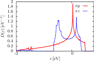
Figure 1: LDA density of states of Sr₂RuO₄ projected on the Ru-$t_{2g}$ orbitals and within the energy window $\mathcal{W}_{s}$ considered in this work to construct the Wannier orbitals.

The Coulomb interaction within the $t_{2g}$ manifold is described with the rotationally invariant Kanamori Hamiltonian:

$$H^{int} = U\sum_{m}n_{m\uparrow}n_{m\downarrow}+(U-2J)\sum_{m\neq m^{\prime}}n_{m\uparrow}n_{m^{\prime}\downarrow}+$$

$$+ (U-3J)\sum_{m>m^{\prime},\sigma}n_{m\sigma}n_{m^{\prime}\sigma}+$$

$$+ J\sum_{m\neq m^{\prime}}(d^{\dagger}_{m\uparrow}d^{\dagger}_{m\downarrow}d_{m^{\prime}\downarrow}d_{m^{\prime}\uparrow}-d^{\dagger}_{m\uparrow}d_{m\downarrow}d^{\dagger}_{m^{\prime}\downarrow}d_{m^{\prime}\uparrow}).$$

Here, $n_{m\sigma}=d^{\dagger}_{m\sigma}d_{m\sigma}$, $U$ is the intraorbital interaction and $J$ is the Hund’s rule coupling. The values of $U$ and $J$ have been estimated in Ref. Mravlje et al. (2011) using the constrained random phase approximation ($U$=2.3eV and $J$=0.4eV, with $J/U$=0.17) and in Ref. Pchelkina et al. (2007) using the constrained local density approximation ($U$=3.1eV and $J$=0.7eV, $J/U$=0.23). If the SOC interaction is not included in the calculations, the local multiplet structure is formed by a doublet $|xy\sigma\rangle$ and a quartet $\{|xz\sigma\rangle,|yz\sigma\rangle\}$, the former having a lower energy. Upon inclusion of the SOC in the DFT calculation, the degeneracy of the quartet is broken leading to three doublets, $|0\rangle,|1\rangle$ and $|2\rangle$. These were calculated by diagonalization of Eq. 4, and can be approximately associated with the states $|J=3/2,m_{J}=\pm 1/2\rangle$, $|J=1/2,m_{J}=\pm 1/2\rangle$, and $|J=3/2,m_{J}=\pm 3/2\rangle$, respectively. The results for the one body energies and the quasiparticle weights are presented in Table 1 for calculations using $U=3.1eV$ and $J/U=0.2$ and $T=5K$ .

	orbital	$\mathbf{\varepsilon^{0}}$ $[\text{eV}]$	$Z_{\mathcal{C}}$	n
Without SOC	$xy$	-0.44	0.61	1.34
	$xz$, $yz$	-0.36	0.56	1.33
With SOC	0	-0.48	0.62	1.38
	1	-0.24	0.53	1.25
	2	-0.42	0.58	1.37

Table 1: Diagonal one-body energies ($\mathbf{\varepsilon^{0}}$), quasiparticle weights ($Z_{\mathcal{C}}$), and occupancies ($n$) corresponding to Wannier orbitals constructed using the energy window $\mathcal{W}_{s}=[-3\,\text{eV},1.3\,\text{eV}]$, both with and without including the SOC. Occupancies and quasiparticle weights correspond to the LDA+RISB calculation with parameters $U=3.1\,\text{eV}$ and $J/U=0.2$.

Although the DFT-DMFT(RISB) results capture the Hund’s metal behavior of the system, showing a strong suppression of the charge fluctuations to states with spin other than the maximum, it underestimates the enhancement of quasiparticle renormalization compared to the one obtained by other numerically exact impurity solvers as CTQMC de’ Medici et al. (2011). This has been established before Behrmann et al. (2012) and is a feature shared with other related techniques like the Gutzwiller approximation Deng et al. (2009); Lanatà et al. (2013, 2015), or the slave-spins formalism Fanfarillo and Bascones (2015). One finds moderate enhancement of the quasiparticle mass $\sim 2$ with a slightly smaller enhancement in the $xy$ orbital. This is different to what is obtained using CTQMC where larger mass enhancements $\sim 4$ are found, even at smaller values of the interaction parameters. Additionally, the fact that the mass enhancement in the xy orbital is smaller may suggest that the slave-bosons are more sensitive to the overall bandwidth than to the low-energy fine-structure in the DOS. Later in the text we will see that in spite of this discrepancies the material trends, as the epitaxial strain is changed, are consistent with what is found using CTQMC.

As it was mentioned in Section I, the renormalized masses (with respect to LDA) of the $\alpha$ and $\beta$ sheets of the Fermi surface have been reported to be $\sim 3$ and $\sim 3.5$, respectively Mackenzie and Maeno (2003). Note that this experimental finding suggests that, altough possible smaller, there must be additional sources of momentum differentiation of the mass enhacement. Indeed, the inequality $\frac{m^{*}}{m_{LDA}}\large|_{\alpha}<\frac{m^{*}}{m_{LDA}}\large|_{\beta}$, or rather $Z_{\alpha}>Z_{\beta}$, is not evident since the Bloch states that conform these sheets have mainly $xz$ and $yz$ symmetry and, as a result, their weight in the correlated subspace lies on degenerate cubic Wannier orbitals. In the following, we show that the spin-orbit coupling enhances the $\vec{k}$ dependence of $\bm{Z}^{QP}_{\mathcal{K}}(\vec{k})$.

When the SOC is turned on, the doublet $|2\rangle$ is lower in energy than the degenerate orbitals $xz$ and $yz$ in the absence of SOC, as can be observed in Table 1. Consequently, while $|2\rangle$ increases its occupancy, which drives the orbital away from half-filling and, in turn, gives place to a larger quasiparticle weight, the opposite happens for $|1\rangle$. To better compare with the calculation done without SOC, it is naturally convenient to analyze the changes in the basis of cubic Wannier functions. We find that both the orbital polarization $n_{xy}-n_{xz}$ and the quasiparticle weights $Z^{\mathcal{C}}_{xy}$ and $Z^{\mathcal{C}}_{xz}$ remain essentially constant upon inclusion of the SOC . This agrees with the CTQMC results of Ref. Kim et al. (2017) and supports the conclusion that the SOC does not affect the coherence scale of Sr₂RuO₄.

The SOC does, however, modify the way the quasiparticle weight varies in $\mathcal{K}$ space. Figures 2(a) and 2(b) present the projected quasiparticle weight ${Z}_{\nu_{F}}^{QP}(\vec{k}_{F})$ (for $\nu_{F}=\alpha,\,\beta,\,\gamma$) [see Eq. (22)] associated with the Fermi surface Bloch states calculated without or with the SOC turned on in the DFT calculations, respectively. In the absence of SOC the only dependence on $\vec{k}$ comes from the difference between $Z^{\mathcal{C}}_{xy}$ and $Z^{\mathcal{C}}_{xz}$. Along each Fermi surface sheet the quasiparticle weight is essentially constant. The inclusion of the SOC leads to a richer momentum differentiation, which is larger at $k_{x}=k_{y}$, consistently with the stronger spin-orbital entanglement experimentally observed by spin-resolved ARPES at that line cut of the Brillouin zone Haverkort et al. (2008); Veenstra et al. (2014). In particular, the relation $Z_{\alpha}>Z_{\beta}$ can only be accounted for in our calculations if the SOC is included.

The effect of the SOC on $Z^{QP}_{\nu_{F}}(\vec{k}_{F})$ can be understood by analyzing the change in the local multiplets and the subsequent induced charge redistribution. Figs. 2(c-e) present the projections of the Bloch states of each sheet onto the different SO multiplets $|0\rangle$, $|1\rangle$ and $|2\rangle$ along the corresponding parametrized angles $\theta_{\alpha}$ and $\theta_{\beta\gamma}$, indicated in Fig. 2(b). The $\gamma$ band has most of its amplitude on the state $|0\rangle$ along almost the whole range of $\theta_{\beta\gamma}$. The $\alpha$ sheet has a larger amplitude on the doublet $|2\rangle$, while the $\beta$ one has it on $|1\rangle$, specially at $\theta_{\alpha}=\pi/4$. The charge redistribution produced by the SOC, which acts to decrease the quasiparticle weight of $|1\rangle$ while incresing that of $|2\rangle$ contributes, therefore, to obtaining $Z_{\alpha}>Z_{\beta}$.

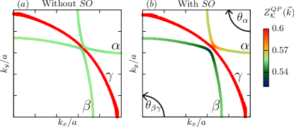
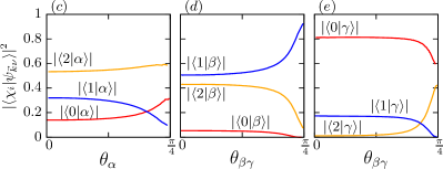
Figure 2: Quasiparticle weight on the Fermi surface calculated without including the spin-orbit interaction $(a)$ or including it $(b)$. $(c)$ Projection of the Bloch states of the $\alpha$ sheet of the Fermi surface on atomic multiplets, as a function of the angle $\theta_{\alpha}$ defined in $(b)$. $(d)$ and $(e)$ present as a function of the angle $\theta_{\beta\gamma}$ the projection on atomic multiplets of the Bloch states from the $\beta$ and $\gamma$ sheets, respectively.

IV Effects of anisotropic strains

Motivated by the recent experimental results reported in Ref. Steppke et al. (2017) and Burganov et al. (2016), in this section we analyze how the electronic correlations evolve in the presence of anisotropic strains. An interesting question is to what extent the Lifshitz transition, in which the Van Hove singularity (VHS) crosses the Fermi level, affects the electronic correlations. We study two situations that have been experimentally addressed and can induce this transition: a biaxial tension that leads to an increase of the lattice parameters $a$ and $b$, and also the response of the system to an uniaxial compression along the [100] direction. In all cases, we use the experimental lattice parameters $a$, $b$ and $c$ and relax within LDA the internal positions of the apical oxygen and of the transition metal atom.

Figure 3(a) shows the evolution of $h/d$ as a function of $a$, where $h$ is the calculated apical oxygen height and $d$=$a/2$ the distance between the Ru and its next oxygen neighbors. For both uniaxial and biaxial strains, $h/d$ evolves towards a more regular octahedron, from 1.07 to 1.03. In the biaxial case, consequently, the splitting between the t_2g bands diminishes. That is, the on-site $xy$ energy decreases while the $\{xz,yz\}$ increases, contributing to transfer charge from the $\{xz,yz\}$ orbitals to the $xy$ one, as confirmed by the evolution of the corresponding occupancies [see Fig. 3(b)] . The uniaxial compression mainly transfers charge from $xz$ to $yz$, the reason being the increased level energy of the $xz$ orbital due to the shorter distances along $x$.

In the presence of a VHS, it is convenient to analyze the strength of the correlations in terms of an effective bandwidth W_eff calculated through the second moment of the density of states, as suggested in Ref. Žitko et al. (2009). The calculated W_eff for the $t_{2g}$ bands are shown in Figs. 3(c) and 3(d). It can be observed that, even for the $xy$ orbital, the W_eff decreases smoothly with $a$. The relative change is only slightly larger in the $\{xz,yz\}$ bands than in the $xy$ one.

In the following, we present how the electronic correlations, as measured by the quasiparticle weight, evolve under the two kinds of deformation mentioned above.

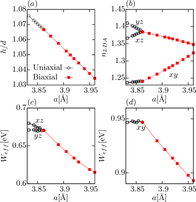
Figure 3: a) $h/d$ as a function of $a$, where $h$ is the height of oxygen octahedron and $d=a/2$ the distance betwen the rutenium atom and its first neighbor oxygen. Empty circles and red filled squares correspond to uniaxial and biaxial stress, respectively. b) Occupancy of Wannier orbitals according to LDA. Effective bandwidth of c) $xz$, $yz$ and d) $xy$ orbitals, as defined in the text.

IV.1 Biaxial strain

Here we present results for strained Sr₂RuO₄ obtained with the formalism introduced in Sec. II and DMFT calculations using CTQMC as impurity solver.

Figures 4(a) and 4(b) show the evolution of the quasiparticle weight associated with the $\{xz,yz\}$ and $xy$ orbitals, respectively, relative to the corresponding values for the unstressed compound (noted as $Z^{(0)}_{\alpha}$), as a function of the lattice parameter $a$. The RISB results depend very weakly on the temperature for $T\lesssim 30K$. The inclusion of the SOC introduces small changes in the quasiparticle weight. In the range of lattice parameters considered, the observed reduction upon including the SOC is less than 1%.

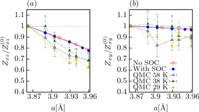
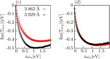
Figure 4: Quasiparticle weight of the $\{xz,yz\}$ $(a)$ and $xy$ orbitals $(b)$ as a function of lattice parameter $a$ calculated using RISB at $T=5K$. Empty red and filled blue symbol datapoints are obtained without and with SOC, respectively. Triangle symbols are CTQMC results without SOC. (c-d) Imaginary part of the self-energy calculated with CTQMC at different temperatures. The interaction parameters are $U=2.3\,\text{eV}$ and $J=0.4\,\text{eV}$.

Both $Z_{xy}$ and $Z_{xz,yz}$ decrease monotonically as $a$ increases from the unstrained case, in line with the monotonic reduction of W_eff shown in Figs. 3(c) and 3(d). The smaller variation rate of $Z_{xy}$ can be associated with two effects. First, the bandwidth reduction of the xy band is percentually smaller than that of the {xz,yz} bands. Second, there is a compensating effect in the correlations generated by the increase in the occupancy of the $xy$ orbital with $a$ which drives it further away from half-filling.

We also performed CTQMC calculations for Sr₂RuO₄ under biaxial strain. For these calculations we used the parameters $U$=2.3eV and $J$=0.4eV. The obtained quasiparticle weights, presented in Fig. 4, indicate, similarly to the RISB results, that the biaxial stress has a stronger effect on the $xz$, $yz$ orbitals. The mass enhancement is computed using a 4th order polynominal fit to the lowest six Matsubara points of the self-energy shown in Fig. 4(c-d). Typically, the values of mass renormalization fluctuate by the order of $10\%$ from DMFT iteration to iteration, hence we present the data with such errorbar. At $T=29\,K$, the effective mass of xz–yz orbitals presents an increment relative to the unstressed compound of $\sim 35\%$ (from 3.4 to 4.6), while that of the xy orbital is of the order of the statistical error, $\sim 10\%$.

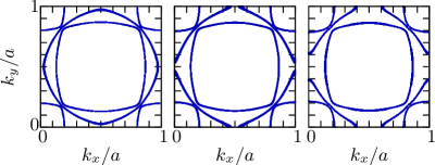
Figure 5: Evolution of the renormalized Fermi surfaces (calculated with SOC) for $a$= 3.862, 3.890, 3.929 Å (from left to right) showing that the system undergoes a Lifshitz transition close to $a$= 3.890 Å.

It is important to point out that the range of values of the lattice parameter $a$ studied, includes the Lifshitz transition of this compound. Figure 5 shows the Fermi surfaces calculated with RISB including the SOC for three different values of $a$= 3.862, 3.890, 3.929 Å. It can be observed that while the electron–like $\beta$ and the hole–like $\alpha$ sheets shrink with increasing $a$, the $\gamma$ one (having mainly $xy$ symmetry) undergoes a Lifshitz transition, changing its character from electron–like to hole–like. This theoretical result agrees with the experimental data reported in Ref. Burganov et al. (2016), obtained for thin films grown on top of different substrates.

The Lifshitz transition occurs already at the LDA level Hsu et al. (2016). The effect of an improved treatment of the correlations through RISB is to slightly decrease the value of $a$ at which the transition takes place ($a_{c}$). More precisely, LDA gives $a_{c}$=3.98 Å, RISB $a_{c}$=3.91 Å and RISB with SOC$a_{c}$=3.89 Å. The value of $a_{c}$ naturally depends on U because this parameter directly affects the occupancy of the $xy$ orbital.

The main conclusion to point out from these results is that there is no significant effect on the electronic correlations, as measured by $Z$, associated with the occurrence of the Lifshitz transition (see also Ref. Han et al. (2016)). This observation is in qualitative agreement with the experimental results of Ref. Burganov et al. (2016).

IV.2 Uniaxial strain

In this section, we study the evolution of the correlation strength as a function of the uniaxial compressive stress $\epsilon_{xx}$. As mentioned before, we use the experimental lattice parameters $a$, $b$ and $c$ Steppke et al. (2017) and relax the internal positions. The results are expected to be symmetric with respect to tensile stress.

Overall, the effect of uniaxial stress on Z is much weaker than in the biaxial case, basically because the induced [100] relative distortion is smaller (up to 0.8 $\%$). On average, the quasiparticle weight of the $t_{2g}$ states slightly increases with uniaxial pressure. Moreover, as the case of biaxial distortion, the correlation strength evolves monotonously through the Lifshitz transition. Figures 6(a) y 6(b) show the evolution of the quasiparticle weigth corresponding to the $xz$, $yz$ and $xy$ states, respectively. We present only the RISB results without SOC, since the effect of SOC is negligible for these small values of compression.

It can be observed that, again, the variation rate of $Z_{xy}$ is much smaller than that of $Z_{xz,yz}$. This is consistent with the almost constant behaviour of the corresponding effective bandwidth and occupancy under uniaxial strain in the former case [see Fig. 3 (d)].

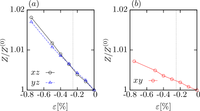
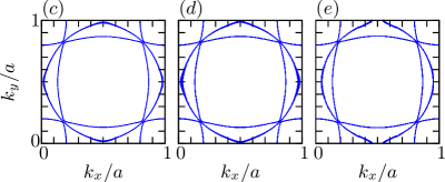
Figure 6: $(a)$ Quasiparticle weight of the orbital $\{xz,yz\}$ as function of the stress $\epsilon_{xx}$ at $T=5\,$K. $(b)$ Quasiparticle weight of the orbital $xy$ as function of the stress $\epsilon_{xx}$. c-e) Evolution of the renormalized Fermi surfaces for the percentage uniaxial stress $\epsilon_{xx}$= 0, -0.2 y -0.5$\%$ (from left to right) showing that the system undergoes a Lifshitz transition close to $\epsilon_{xx}$=0.2$\%$ around the $(\frac{\pi}{2a},0)$ point.

V Conclusions

In this article we presented an implementation of the multiorbital slave-boson rotationally invariant (RISB) quantum impurity solver within the LDA+DMFT approach to ab initio calculations of strongly correlated systems. The main disadvantage of the RISB solver is that in general it can only be trusted at a qualitative level and that it fails to describe non-Fermi liquid behaviors besides trivial insulating phases. Its main advantages, compared to other numerically exact solvers as Quantum Monte Carlo, are its much lower computational cost at low temperatures which allows to rapidly explore a wide range of parameters and materials, and the abilty of easily handling off-diagonal hybridizations at arbitrary low temperatures in problems that in general give place to a sign problem in CTQMC. It can therefore be used as a tool to explore and identify correlated regimes worth of a more detailed study using other techniques as CTQMC or numerical renormalization group approaches. An important result of our implementation is that we obtained transformation relations between physical quantities, as the quasiparticle mass renormalization, in the local correlated space and their counterparts in Bloch space. This transformation allows to obtain the momentum dependence of the quasiparticle mass renormalization independently of the quantum impurity solver used to treat the DMFT equations. We applied the RISB approach to study the electronic correlations, as measured by the quasiparticle mass enhancement, of Sr₂RuO₄. We found that it is necessary to include the spin-orbit coupling in the DFT calculations to explain the experimentally observed mass enhancement differentiation between the $\alpha$ and $\beta$ sheets of the Fermi surface. We also find that the SOC strongly enhances the momentum dependence of the quasiparticle weight on both sheets while the $\gamma$ sheet is largely unaffected.

A biaxial stretching of the compound on the $a-b$ plane leads to a monotonic increase of the mass enhancement that is larger for the $xz$ and $yz$ orbitals, which determine the mass enhancement of the $\alpha$ and $\beta$ Fermi sheets, than for the $xy$ orbital, which determines the mass enhancement of the $\gamma$ Fermi sheet. While the sample suffers a Lifshitz transition for $a=b\sim 3.9$Å, we did not find any significant change of behavior of the mass enhancement across it. We also performed calculations using the numerically exact CTQMC solver which confirmed the absence of any dramatic effect of the electronic correlations at the Lifshitz transition.

Finally, we analyzed the behavior of the mass enhancement when the sample is under uniaxial strain. As in the biaxial case, we found a monotonic behavior with no significant features across the Lifshitz transition.

Appendix A Inverse relations

The inverse of Eq. (18) can be obtained by applying $\bm{P}(\vec{k})$ and $\bm{P}^{\dagger}(\vec{k})$ at left and right, respectively, and using $\bm{P}(\vec{k})\bm{P}^{\dagger}(\vec{k})=\bm{1}_{\mathcal{C}}$, it reads:

$$\bm{P}(\vec{k})\bm{Z}^{-1}_{\mathcal{K}}(\vec{k})\bm{P}^{\dagger}(\vec{k})=\bm{Z}_{\mathcal{C}}^{-1}$$ (24)

The asymmetry between Eqs. (18) and (24) comes from the fact that the transformations $\bm{P}(\vec{k})$ are not unitary in the general case.

Based on Eq. (18), we define:

$$\bm{R}^{-1}_{\mathcal{K}}(\vec{k})=\bm{1}_{\mathcal{K}(\vec{k})}-\bm{P}^{\dagger}(\vec{k})\bm{P}(\vec{k})+\bm{P}^{\dagger}(\vec{k})\bm{R}_{\mathcal{C}}^{-1}\bm{P}(\vec{k})$$ (25)

and in analogy with Eq. (24) we obtain:

$$\bm{P}(\vec{k})\bm{R}^{-1}_{\mathcal{K}}(\vec{k})\bm{P}^{\dagger}(\vec{k}) =\bm{R}_{\mathcal{C}}^{-1}.$$ (26)

From Eq. (25) it can be shown by direct calculation that the quasiparticle mass renormalization in $\mathcal{K}$ space satisfies

$$\bm{Z}_{\mathcal{K}}(\vec{k})=\bm{R}_{\mathcal{K}}(\vec{k})\bm{R}_{\mathcal{K}}^{\dagger}(\vec{k}).$$ (27)

The relation between transformation matrices given by Eq. (25) is consistent with the relations between quasiparticle and physical Green’s functions in both $\mathcal{K}$ and $\mathcal{C}$ spaces. To show this we transform Eq. (16) to $\mathcal{C}$ space. We first derive the following relation between the transformation matrices in $\mathcal{C}$ and $\mathcal{K}$.

$$\bm{P}(\vec{k})\bm{R}_{\mathcal{K}}^{-1}(\vec{k})=\bm{R}_{\mathcal{C}}^{-1}\bm{P}(\vec{k}),$$ (28)

by applying $\bm{P}(\vec{k})$ to the left of Eq. (25). Similarly, we also obtain:

$$\bm{R}_{\mathcal{K}}^{{\dagger}-1}(\vec{k})\bm{P}^{\dagger}(\vec{k})=\bm{P}^{\dagger}(\vec{k})\bm{R}^{{\dagger}-1}_{\mathcal{C}}.$$ (29)

From Eq. (16) it follows that:

$$\bm{G_{qp}}(\vec{k},i\omega_{n})=\bm{R}_{\mathcal{K}}^{-1}(\vec{k})\bm{G}(\vec{k},i\omega_{n})[\bm{R}_{\mathcal{K}}^{\dagger}]^{-1}(\vec{k}).$$ (30)

We project this equation to $\mathcal{C}$ multiplying at left by $\bm{P}(\vec{k})$, at right by $\bm{P}^{\dagger}(\vec{k})$ and summing over $\vec{k}$:

$$\bm{G_{qp}^{loc}}(i\omega_{n})=\sum_{\vec{k}}\bm{P}(\vec{k})\bm{R}_{\mathcal{K}}^{-1}(\vec{k})\bm{G}(\vec{k},i\omega_{n})\bm{R}_{\mathcal{K}}^{{\dagger}-1}(\vec{k})\bm{P}^{\dagger}(\vec{k}).$$

Using Eqs. (28) and Eq. (29), we have:

$$\bm{G_{qp}^{loc}}(i\omega_{n})=\sum_{\vec{k}}\bm{R}_{\mathcal{C}}^{-1}\bm{P}(\vec{k})\bm{G}(\vec{k},i\omega_{n})\bm{P}^{\dagger}(\vec{k})\bm{R}^{{\dagger}-1}_{\mathcal{C}}$$

$$=\bm{R}_{\mathcal{C}}^{-1}\Big{(}\sum_{\vec{k}}\bm{P}(\vec{k})\bm{G}(\vec{k},i\omega_{n})\bm{P}^{\dagger}(\vec{k})\Big{)}\bm{R}^{{\dagger}-1}_{\mathcal{C}}$$

$$=\bm{R}_{\mathcal{C}}^{-1}\bm{G}^{loc}(i\omega_{n})\bm{R}^{{\dagger}-1}_{\mathcal{C}},$$ (31)

and finally

$$\bm{R}_{\mathcal{C}}\bm{G_{qp}^{loc}}(i\omega_{n})\bm{R}^{\dagger}_{\mathcal{C}}=\bm{G^{loc}}(i\omega_{n}),$$ (32)

which is the expected relation between the physical and the quasiparticle Green’s functions in $\mathcal{C}$.

Appendix B Derivation of Eq. (19).

The quasiparticle lattice Green’s function can be computed using the DFT+DMFT equations and the self-energy obtained in the RISB saddle-point approximation. To this aim, we substitute in Eq. (1) the self-energy given by Eq. (10). The terms linear in frequency and in the chemical potential read (in the following we omit the dependence in $\vec{k}$ of $\bm{P}$ and $\bm{R}_{\mathcal{K}}$):

$$(i\omega_{n}+\mu)[\bm{1}_{\mathcal{K}(\vec{k})}-\bm{P}^{\dagger}(\bm{1}_{\mathcal{C}}-\bm{Z}_{\mathcal{C}}^{-1})\bm{P}]=(i\omega_{n}+\mu)\bm{Z}^{-1}_{\mathcal{K}},$$ (33)

where we have used Eq. (18). The term proportional to $\mathbf{\Lambda}_{\mathcal{C}}$ reads:

$$\bm{P}^{\dagger}\bm{R}^{{\dagger}-1}_{\mathcal{C}}\bm{\Lambda}_{\mathcal{C}}\bm{R}^{-1}_{\mathcal{C}}\bm{P}=\bm{R}^{{\dagger}-1}_{\mathcal{K}}\bm{P}^{\dagger}\bm{\Lambda}_{\mathcal{C}}\bm{P}\bm{R}^{-1}_{\mathcal{K}},$$ (34)

where the equality follows using Eqs. (28) and (29). The other terms are:

$$-\bm{\varepsilon}(\vec{k})+\bm{P}^{\dagger}\big{(}\bm{\varepsilon^{0}}+\bm{\Sigma^{dc}}\big{)}\bm{P}.$$ (35)

The summation of these terms and use of Eq. (16) leads to Eq. (19).

Appendix C Application to SrVO₃

Here we present as a benchmark a comparison between results obtained with LDA+RISB and LDA+DMFT (CTQMC) for the compound SrVO₃. We use values of $U=4.5\,$eV and $J=0.6\,$eV, and construct Wannier functions for the $t_{2g}$ bands within the energy window $[-1,2]\,$eV. Fig. 7 presents the spectral density as function of the energy for each of the three-fold degenerated $t_{2g}$ Wannier orbitals. It can be observed that the RISB method provides a reasonably good approximation at low energies in spite of subestimating the bandwith renormalization. The values of $Z$ obtained are $\sim 0.5$ and $\sim 0.65$ for CTQMC and RISB, respectively.

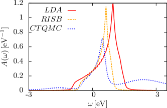
Figure 7: Density of states projected on the t${}_{2}g$ Wannier orbital, calculated using LDA, LDA+DMFT(RISB), and LDA+DMFT(CTQMC)