A Differential Privacy Mechanism Design
Under Matrix-Valued Query

Abstract

Traditionally, differential privacy mechanism design has been tailored for a scalar-valued query function. Although many mechanisms such as the Laplace and Gaussian mechanisms can be extended to a matrix-valued query function by adding i.i.d. noise to each element of the matrix, this method is often sub-optimal as it forfeits an opportunity to exploit the structural characteristics typically associated with matrix analysis. In this work, we consider the design of differential privacy mechanism specifically for a matrix-valued query function. The proposed solution is to utilize a matrix-variate noise, as opposed to the traditional scalar-valued noise. Particularly, we propose a novel differential privacy mechanism called the Matrix-Variate Gaussian (MVG) mechanism, which adds a matrix-valued noise drawn from a matrix-variate Gaussian distribution. We prove that the MVG mechanism preserves $(\epsilon,\delta)$-differential privacy, and show that it allows the structural characteristics of the matrix-valued query function to naturally be exploited. Furthermore, due to the multi-dimensional nature of the MVG mechanism and the matrix-valued query, we introduce the concept of directional noise, which can be utilized to mitigate the impact the noise has on the utility of the query. Finally, we demonstrate the performance of the MVG mechanism and the advantages of directional noise using three matrix-valued queries on three privacy-sensitive datasets. We find that the MVG mechanism notably outperforms four previous state-of-the-art approaches, and provides comparable utility to the non-private baseline. Our work thus presents a promising prospect for both future research and implementation of differential privacy for matrix-valued query functions.

1 Introduction

Differential privacy [2, 3, 4] has become the gold standard for a rigorous privacy guarantee, and there has been the development of many differentially-private mechanisms. Some popular mechanisms include the classical Laplace mechanism [3] and the Exponential mechanism [5]. In addition, there are other mechanisms that build upon these two classical ones such as those based on data partition and aggregation [6, 7, 8, 9, 10, 11, 12, 13, 14, 15, 16], and those based on adaptive queries [17, 18, 19, 20, 21, 22, 23]. From this observation, differentially-private mechanisms may be categorized into two groups: the basic mechanisms, and the derived mechanisms. The basic mechanisms’ privacy guarantee is self contained, whereas the derived mechanisms’ privacy guarantee is achieved through a combination of basic mechanisms, composition theorems, and the post-processing invariance property [24].

In this work, we consider the design of a basic mechanism for matrix-valued query functions. Existing basic mechanisms for differential privacy are designed usually for scalar-valued query functions. However, in many practical settings, the query functions are multi-dimensional and can be succinctly represented as matrix-valued functions. Examples of matrix-valued query functions in the real-world applications include the covariance matrix [25, 26, 27], the kernel matrix [28], the adjacency matrix [29], the incidence matrix [29], the rotation matrix [30], the Hessian matrix [31], the transition matrix [32], and the density matrix [33], which find applications in statistics [34], machine learning [35], graph theory [29], differential equations [31], computer graphics [30], probability theory [32], quantum mechanics [33], and many other fields [36].

One property that distinguishes the matrix-valued query functions from the scalar-valued query functions is the relationship and interconnection among the elements of the matrix. One may naively treat these matrices as merely a collection of scalar values, but that could prove sub-optimal since the structure and relationship among these scalar values are often informative and essential to the understanding and analysis of the system. For example, in graph theory, the adjacency matrix is symmetric for an undirected graph, but not for a directed graph [29] – an observation which is implausible to extract from simply looking at the collection of elements without considering how they are arranged in the matrix.

In differential privacy, the traditional method for dealing with a matrix-valued query function is to extend a scalar-valued mechanism by adding independent and identically distributed (i.i.d.) noise to each element of the matrix [3, 2, 37]. However, this method fails to utilize the structural characteristics of the matrix-valued noise and query function. Although some advanced methods have explored this possibility in an iterative/procedural manner [17, 18], the structural characteristics of the matrices are still largely under-investigated. This is partly due to the lack of a basic mechanism that is directly designed for matrix-valued query functions, making the utilization of matrix structures and application of available tools in matrix analysis challenging.

In this work, we formalize the study of the matrix-valued differential privacy, and present a new basic mechanism that can readily exploit the structural characteristics of the matrices – the Matrix-Variate Gaussian (MVG) mechanism. The high-level concept of the MVG mechanism is simple – it adds a matrix-variate Gaussian noise scaled to the $L_{2}$-sensitivity of the matrix-valued query function (cf. Figure 1). We rigorously prove that the MVG mechanism guarantees $(\epsilon,\delta)$-differential privacy, and show that, with the MVG mechanism, the structural characteristics of the matrix-valued query functions can readily be incorporated into the mechanism design. Specifically, we present an example of how the MVG mechanism can yield greater utility by exploiting the positive-semi definiteness of the matrix-valued query function. Moreover, due to the multi-dimensional nature of the noise and the query function, the MVG mechanism allows flexibility in the design via the novel notion of directional noise. An important consequence of the concept of directional noise is that the matrix-valued noise in the MVG mechanism can be devised to affect certain parts of the matrix-valued query function less than the others, while providing the same privacy guarantee. In practice, this property could be advantageous as the noise can be tailored to have minimal impact on the intended utility. We present simple algorithms to incorporate the directional noise into the differential privacy mechanism design, and theoretically present the optimal design for the MVG mechanism with directional noise that maximizes the power-to-noise ratio of the mechanism output.

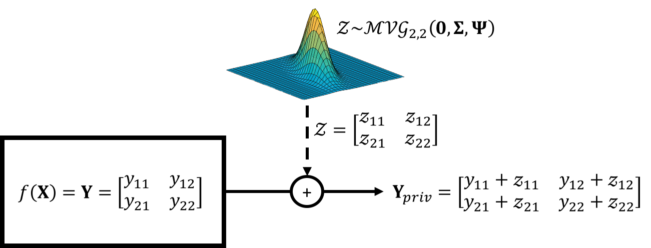
Figure 1: Given a matrix-valued query function $f(\mathbf{X})\in\mathbb{R}^{m\times n}$, the MVG mechanism adds a matrix-valued noise drawn from the matrix-variate Gaussian distribution $\mathcal{MVG}_{m,n}(\mathbf{0},\boldsymbol{\Sigma},\boldsymbol{\Psi})$ to guarantee $(\epsilon,\delta)$-differential privacy. The schematic shows an example when $m=n=2$.

Finally, to illustrate the effectiveness of the MVG mechanism, we conduct experiments on three privacy-sensitive real-world datasets – Liver Disorders [38, 39], Movement Prediction [40], and Cardiotocography [38, 41]. The experiments include three tasks involving matrix-valued query functions – regression, finding the first principal component, and covariance estimation. The results show that the MVG mechanism can evidently outperform four prior state-of-the-art mechanisms – the Laplace mechanism, the Gaussian mechanism, the Exponential mechanism, and the JL transform – in utility in all experiments, and can provide the utility similar to that achieved with the non-private methods, while guaranteeing differential privacy.

To summarize, the main contributions are as follows.

• We formalize the study of matrix-valued query functions in differential privacy and introduce the novel Matrix-Variate Gaussian (MVG) mechanism.

• We rigorously prove that the MVG mechanism guarantees $(\epsilon,\delta)$-differential privacy.

• We show that exploiting the structural characteristic of the matrix-valued query function can improve the utility performance of the MVG mechanism.

• We introduce a novel concept of directional noise, and propose two simple algorithms to implement this novel concept with the MVG mechanism.

• We theoretically exhibit how the directional noise can be devised to provide the maximum utility from the MVG mechanism.

• We evaluate our approach on three real-world datasets and show that our approach can outperform four prior state-of-the-art mechanisms in all experiments, and yields utility performance close to the non-private baseline.

2 Prior Works

Existing mechanisms for differential privacy may be categorized into two types: the basic [3, 2, 42, 5, 37, 43, 44, 45, 46]; and the derived mechanisms [16, 47, 6, 7, 8, 9, 10, 11, 12, 13, 14, 15, 48, 49, 18, 17, 50, 51, 52, 53, 54, 55, 19, 20, 17, 23, 22]. Since our work concerns the basic mechanism design, we focus our discussion on this type, and provide a general overview of the other.

2.1 Basic Mechanisms

Basic mechanisms are those whose privacy guarantee is self-contained, i.e. it does not deduce the guarantee from another mechanism. Here, we discuss four popular existing basic mechanisms: the Laplace mechanism, the Gaussian mechanism, the Johnson-Lindenstrauss transform method, and the Exponential mechanism.

2.1.1 Laplace Mechanism

The classical Laplace mechanism [3] adds noise drawn from the Laplace distribution scaled to the $L_{1}$-sensitivity of the query function. It was initially designed for a scalar-valued query function, but can be extended to a matrix-valued query function by adding i.i.d. Laplace noise to each element of the matrix. The Laplace mechanism provides the strong $\epsilon$-differential privacy guarantee and is relatively simple to implement. However, its generalization to a matrix-valued query function does not automatically utilize the structure of the matrices involved.

2.1.2 Gaussian Mechanism

The Gaussian mechanism [37, 2, 43] uses i.i.d. additive noise drawn from the Gaussian distribution scaled to the $L_{2}$-sensitivity of the query function. The Gaussian mechanism guarantees $(\epsilon,\delta)$-differential privacy. It suffers from the same limitation as the Laplace mechanism when extended to a matrix-valued query function, i.e. it does not automatically consider the structure of the matrices.

2.1.3 Johnson-Lindenstrauss Transform

The Johnson-Lindenstrauss (JL) transform method [42] uses multiplicative noise to guarantee $(\epsilon,\delta)$-differential privacy. It is, in fact, a rare basic mechanism designed for a matrix-valued query function. Despite its promise, previous works show that the JL transform method can be applied to queries with certain properties only, as we discuss here.

• Blocki et al. [42] use a random matrix, whose entries are drawn i.i.d. from a Gaussian distribution, and the method is applicable to the Laplacian of a graph and the covariance matrix.

• Blum and Roth [44] use a hash function that implicitly represents the JL transform, and the method is suitable for a sparse query.

• Upadhyay [45, 46] uses a multiplicative combination of random matrices to provide a JL transform that is applicable to any matrix-valued query function whose singular values are all above a minimum threshold.

Among these methods, Upadhyay’s works [45, 46] stand out as possibly the most general. In our experiments, we show that our approach can yield higher utility for the same privacy budget than these methods.

2.1.4 Exponential Mechanism

In contrast to additive and multiplicative noise used in previous approaches, the Exponential mechanism uses noise introduced via the sampling process [5]. The Exponential mechanism draws its query answers from a custom probability density function designed to preserve $\epsilon$-differential privacy. To provide reasonable utility, the Exponential mechanism designs its sampling distribution based on the quality function, which indicates the utility score of each possible sample. Due to its generality, the Exponential mechanism has been utilized for many types of query functions, including the matrix-valued query functions. We experimentally compare our approach to the Exponential mechanism, and show that, with slightly weaker privacy guarantee, our method can yield significant utility improvement.

Finally, we conclude that our method differs from the four existing basic mechanisms as follows. In contrast with the i.i.d. noise in the Laplace and Gaussian mechanisms, the MVG mechanism allows a non-i.i.d. noise (cf. Section 5). As opposed to the multiplicative noise in the JL transform and the sampling noise in the Exponential mechanism, the MVG mechanism uses an additive noise for matrix-valued query functions.

2.2 Derived Mechanisms

Derived mechanisms are those whose privacy guarantee is deduced from other basic mechanisms via the composition theorems and the post-processing invariance property [24]. Derived mechanisms are often designed to provide better utility by exploiting some properties of the query function or of the data. Blocki et al. [42] also define a similar categorization with the term “revised algorithm”.

The general techniques used by derived mechanisms are often translatable among basic mechanisms, including our MVG mechanism. Given our focus on a novel basic mechanism, these techniques are less relevant to our work, and we leave the investigation of integrating them into the MVG framework in future work. Some of the popular techniques used by derived mechanisms are summarized here.

2.2.1 Sensitivity Control

This technique avoids the worst-case sensitivity in basic mechanisms by using variant concepts of sensitivity. Examples include the smooth sensitivity framework [16] and elastic sensitivity [47].

2.2.2 Data Partition and Aggregation

This technique uses data partition and aggregation to produce more accurate query answers [6, 7, 8, 9, 10, 11, 12, 13, 14, 15]. The partition and aggregation processes are done in a differentially-private manner either via the composition theorems and the post-processing invariance property [24], or with a small extra privacy cost. Hay et al. [48] nicely summarize many works that utilize this concept.

2.2.3 Non-uniform Data Weighting

This technique lowers the level of perturbation required for the privacy protection by weighting each data sample or dataset differently [49, 18, 17, 50]. The rationale is that each sample in a dataset, or each instance of the dataset itself, has a heterogeneous contribution to the query output. Therefore, these mechanisms place a higher weight on the critical samples or instances of the database to provide better utility.

2.2.4 Data Compression

This approach reduces the level of perturbation required for differential privacy via dimensionality reduction. Various dimensionality reduction methods have been proposed. For example, Kenthapadi et al. [51], Xu et al. [53], and Li et al. [54] use random projection; Chanyaswad et al. [52] and Jiang et al. [55] use principal component analysis (PCA); Xiao et al. [6] use wavelet transform; and Acs et al. [15] use lossy Fourier transform.

2.2.5 Adaptive Queries

The derived mechanisms based on adaptive queries use prior and/or auxiliary information to improve the utility of the query answers. Examples include the matrix mechanism [19, 20], the multiplicative weights mechanism [17, 18], the low-rank mechanism [21], boosting [23], and the sparse vector technique [37, 22].

Finally, we conclude with three main observations. First, the MVG mechanism falls into the category of basic mechanism. Second, techniques used in derived mechanisms are generally applicable to multiple basic mechanisms, including our novel MVG mechanism. Third, therefore, for fair comparison, we will compare the MVG mechanism with the four state-of-the-art basic mechanisms presented in this section.

3 Background

We begin with a discussion of basic concepts pertaining to the MVG mechanism for matrix-valued query.

3.1 Matrix-Valued Query

In our analysis, we use the term dataset interchangeably with database, and represent it with the matrix $\mathbf{X}$. The matrix-valued query function, $f(\mathbf{X})\in\mathbb{R}^{m\times n}$, has $m$ rows and $n$ columns. We define the notion of neighboring datasets $\{\mathbf{X}_{1},\mathbf{X}_{2}\}$ as two datasets that differ by a single record, and denote it as $d(\mathbf{X}_{1},\mathbf{X}_{2})=1$. We note, however, that although the neighboring datasets differ by only a single record, $f(\mathbf{X}_{1})$ and $f(\mathbf{X}_{2})$ may differ in every element.

We denote a matrix-valued random variable with the calligraphic font, e.g. $\mathcal{Z}$, and its instance with the bold font, e.g. $\mathbf{Z}$. Finally, as will become relevant later, we use the columns of $\mathbf{X}$ to denote the records (samples) in the dataset.

3.2 $(\epsilon,\delta)$-Differential Privacy

In the paradigm of data privacy, differential privacy [4, 2] provides a rigorous privacy guarantee, and has been widely adopted in the community [24]. Differential privacy guarantees that the involvement of any one particular record of the dataset would not drastically change the query answer.

Definition 1.

A mechanism $\mathcal{A}$ on a query function $f(\cdot)$ is $(\epsilon,\delta)$- differentially-private if for all neighboring datasets $\{\mathbf{X}_{1},\mathbf{X}_{2}\}$, and for all possible measurable matrix-valued outputs $\mathbf{Y}\subseteq\mathbb{R}^{m\times n}$,

$$\Pr[\mathcal{A}(f(\mathbf{X}_{1}))\in\mathbf{Y}]\leq e^{\epsilon}\Pr[\mathcal{A}(f(\mathbf{X}_{2}))\in\mathbf{Y}]+\delta.$$

3.3 Matrix-Variate Gaussian Distribution

One of our main innovations is the use of the noise drawn from a matrix-variate probability distribution. More specifically, in the MVG mechanism, the additive noise is drawn from the matrix-variate Gaussian distribution, defined as follows [56, 57, 58, 59, 60, 61].

Definition 2.

An $m\times n$ matrix-valued random variable $\mathcal{X}$ has a matrix-variate Gaussian distribution, denoted as $\mathcal{MVG}_{m,n}(\mathbf{M},\boldsymbol{\Sigma},\boldsymbol{\Psi})$, if it has the probability density function:

$$p_{\mathcal{X}}(\mathbf{X})=\frac{\exp\{-\frac{1}{2}\mathrm{tr}[\boldsymbol{\Psi}^{-1}(\mathbf{X}-\mathbf{M})^{T}\boldsymbol{\Sigma}^{-1}(\mathbf{X}-\mathbf{M})]\}}{(2\pi)^{mn/2}\left|\boldsymbol{\Psi}\right|^{m/2}\left|\boldsymbol{\Sigma}\right|^{n/2}},$$

where $\mathrm{tr}(\cdot)$ is the matrix trace [62], $\left|\cdot\right|$ is the matrix determinant [62], $\mathbf{M}\in\mathbb{R}^{m\times n}$ is the mean, $\boldsymbol{\Sigma}\in\mathbb{R}^{m\times m}$ is the row-wise covariance, and $\boldsymbol{\Psi}\in\mathbb{R}^{n\times n}$ is the column-wise covariance.

Noticeably, the probability density function (pdf) of $\mathcal{MVG}_{m,n}(\mathbf{M},\boldsymbol{\Sigma},\boldsymbol{\Psi})$ looks similar to that of the $m$-dimensional multivariate Gaussian distribution, $\mathcal{N}_{m}(\boldsymbol{\mu},\boldsymbol{\Sigma})$. Indeed, $\mathcal{MVG}_{m,n}(\mathbf{M},\boldsymbol{\Sigma},\boldsymbol{\Psi})$ is a generalization of $\mathcal{N}_{m}(\boldsymbol{\mu},\boldsymbol{\Sigma})$ to a matrix-valued random variable. This leads to a few notable additions. First, the mean vector $\boldsymbol{\mu}$ now becomes the mean matrix $\mathbf{M}$. Second, in addition to the traditional row-wise covariance matrix $\boldsymbol{\Sigma}$, there is also the column-wise covariance matrix $\boldsymbol{\Psi}$. The latter addition is due to the fact that, not only could the rows of the matrix be distributed non-uniformly, but also could its columns.

We may intuitively explain this addition as follows. If we draw $n$ i.i.d. samples from $\mathcal{N}_{m}(\mathbf{0},\boldsymbol{\Sigma})$ denoted as $\mathbf{x}_{1},\mathbf{x}_{2},\ldots,\mathbf{x}_{n}\in\mathbb{R}^{m}$, and concatenate them into a matrix $\mathbf{X}=[\mathbf{x}_{1},\mathbf{x}_{2},\ldots,\mathbf{x}_{n}]\in\mathbb{R}^{m\times n}$, then, it can be shown that $\mathbf{X}$ is drawn from $\mathcal{MVG}_{m,n}(\mathbf{0},\boldsymbol{\Sigma},\mathbf{I})$, where $\mathbf{I}$ is the identity matrix [56]. However, if we consider the case when the columns of $\mathbf{X}$ are not i.i.d., and are distributed with the covariance $\boldsymbol{\Psi}$ instead, then, it can be shown that this is distributed according to $\mathcal{MVG}_{m,n}(\mathbf{0},\boldsymbol{\Sigma},\boldsymbol{\Psi})$ [56].

3.4 Relevant Matrix Algebra Theorems

We recite major theorems in matrix algebra that are essential to the subsequent analysis and discussion as follows.

Theorem 1 (Singular value decomposition (SVD) [62]).

A matrix $\mathbf{A}\in\mathbb{R}^{m\times n}$ can be decomposed into two unitary matrices $\mathbf{W}_{1}\in\mathbb{R}^{m\times m},\mathbf{W}_{2}\in\mathbb{R}^{n\times n}$, and a diagonal matrix $\boldsymbol{\Lambda}$, whose diagonal elements are ordered non-increasingly downward. These diagonal elements are the singular values of $\mathbf{A}$ denoted as $\sigma_{1}\geq\sigma_{2}\geq\cdots\geq 0$, and $\mathbf{A}=\mathbf{W}_{1}\boldsymbol{\Lambda}\mathbf{W}_{2}^{T}$.

Lemma 1 (Laurent-Massart [63]).

For a matrix-variate random variable $\mathcal{N}\sim\mathcal{MVG}_{m,n}(\mathbf{0},\mathbf{I}_{m},\mathbf{I}_{n})$, $\delta\in[0,1]$, and $\zeta(\delta)=2\sqrt{-mn\ln\delta}-2\ln\delta+mn$, the following inequality holds:

$$\Pr[\left\|\mathcal{N}\right\|_{F}^{2}\leq\zeta(\delta)^{2}]\geq 1-\delta,$$

where $\left\|\cdot\right\|_{F}$ is the Frobenius norm of a matrix.

Lemma 2 (Merikoski-Sarria-Tarazaga [64]).

The non-increasingly ordered singular values of a matrix $\mathbf{A}\in\mathbb{R}^{m\times n}$ have the values of

$$0\leq\sigma_{i}\leq\frac{\left\|\mathbf{A}\right\|_{F}}{\sqrt{i}},$$

where $\left\|\cdot\right\|_{F}$ is the Frobenius norm of a matrix.

Lemma 3 (von Neumann [65]).

Let $\mathbf{A},\mathbf{B}\in\mathbb{R}^{m\times n}$, and let $\sigma_{i}(\mathbf{A})$ and $\sigma_{i}(\mathbf{B})$ be the non-increasingly ordered singular values of $\mathbf{A}$ and $\mathbf{B}$, respectively. Then

$$\mathrm{tr}(\mathbf{A}\mathbf{B}^{T})\leq\Sigma_{i=1}^{r}\sigma_{i}(\mathbf{A})\sigma_{i}(\mathbf{B}),$$

where $r=\min\{m,n\}$.

Lemma 4 (Trace magnitude bound [66]).

Let $\mathbf{A}\in\mathbb{R}^{m\times n}$, and let $\sigma_{i}(\mathbf{A})$ be the non-increasingly ordered singular values of $\mathbf{A}$. Then

$$\left|\mathrm{tr}(\mathbf{A})\right|\leq\sum_{i=1}^{r}\sigma_{i}(\mathbf{A}),$$

where $r=\min\{m,n\}$.

Lemma 5 (Hadamard’s inequality [67]).

Let $\mathbf{A}\in\mathbb{R}^{m\times m}$ be non-singular and $\mathbf{a}_{i}$ be the $i^{th}$ column vector of $\mathbf{A}$ . Then,

$$\left|\mathbf{A}\right|^{2}\leq\prod_{i=1}^{m}\left\|\mathbf{a}_{i}\right\|^{2},$$

where $\left|\cdot\right|$ is the matrix determinant [62], and $\left\|\cdot\right\|$ is the $L_{2}$-norm of a vector.

4 MVG Mechanism: Differential Privacy with Matrix-Valued Query

Matrix-valued query functions are different from their scalar counterparts in terms of the vital information contained in how the elements are arranged in the matrix. To fully exploit these structural characteristics of matrix-valued query functions, we present a novel mechanism for matrix-valued query functions: the Matrix-Variate Gaussian (MVG) mechanism.

4.1 Definitions

First, let us introduce the sensitivity of the matrix-valued query function used in the MVG mechanism.

Definition 3 (Sensitivity).

Given a matrix-valued query function $f(\mathbf{X})\in\mathbb{R}^{m\times n}$, define the $L_{2}$-sensitivity as,

$$s_{2}(f)=\sup_{d(\mathbf{X}_{1},\mathbf{X}_{2})=1}\left\|f(\mathbf{X}_{1})-f(\mathbf{X}_{2})\right\|_{F},$$

where $\left\|\cdot\right\|_{F}$ is the Frobenius norm [62].

Then, we present the MVG mechanism as follows.

Definition 4 (MVG mechanism).

Given a matrix-valued query function $f(\mathbf{X})\in\mathbb{R}^{m\times n}$, and a matrix-valued random variable $\mathcal{Z}\sim\mathcal{MVG}_{m,n}(\mathbf{0},\boldsymbol{\Sigma},\boldsymbol{\Psi})$, the MVG mechanism is defined as,

$$\mathcal{MVG}(f(\mathbf{X}))=f(\mathbf{X})+\mathcal{Z},$$

where $\boldsymbol{\Sigma}$ is the row-wise covariance matrix, and $\boldsymbol{\Psi}$ is the column-wise covariance matrix.

Note that so far, we have not specified how to pick $\boldsymbol{\Sigma}$ and $\boldsymbol{\Psi}$ according to the sensitivity $s_{2}(f)$ in the MVG mechanism. We discuss the explicit form of $\boldsymbol{\Sigma}$ and $\boldsymbol{\Psi}$ next.

As the additive matrix-valued noise of the MVG mechanism is drawn from $\mathcal{MVG}_{m,n}(\mathbf{0},\boldsymbol{\Sigma},\boldsymbol{\Psi})$, the parameters to be designed for the mechanism are the covariance matrices $\boldsymbol{\Sigma}$ and $\boldsymbol{\Psi}$. In the following discussion, we derive the sufficient conditions on $\boldsymbol{\Sigma}$ and $\boldsymbol{\Psi}$ such that the MVG mechanism preserves $(\epsilon,\delta)$-differential privacy. Furthermore, since one of the motivations of the MVG mechanism is to facilitate the exploitation of the structural characteristics of the matrix-value query, we demonstrate how the structural knowledge about the matrix-value query can improve the sufficient condition for the MVG mechanism. The term improve here certainly requires further specification, and we provide such clarification when the context is appropriate later in this section.

Hence, the subsequent discussion proceeds as follows. First, we present a sufficient condition for the values of $\boldsymbol{\Sigma}$ and $\boldsymbol{\Psi}$ to ensure that the MVG mechanism preserves $(\epsilon,\delta)$-differential privacy without assuming structural knowledge about the matrix-valued query. Second, we present an alternative sufficient condition for $\boldsymbol{\Sigma}$ and $\boldsymbol{\Psi}$ to ensure that the MVG mechanism preserves $(\epsilon,\delta)$-differential privacy with the assumption that the matrix-value query is symmetric positive semi-definite (PSD). Finally, we rigorously prove that, by incorporating the knowledge of positive semi-definiteness about the matrix-value query, we improve the sufficient condition to guarantee $(\epsilon,\delta)$-differential privacy with the MVG mechanism.

4.2 Differential Privacy Analysis for General Matrix-Valued Query (No Structural Assumption)

$\mathbf{X}$	database/dataset whose columns are data records and rows are attributes/features.
$\mathcal{MVG}_{m,n}(\mathbf{0},\boldsymbol{\Sigma},\boldsymbol{\Psi})$	$m\times n$ matrix-variate Gaussian distribution with zero mean, the row-wise covariance $\boldsymbol{\Sigma}$, and the column-wise covariance $\boldsymbol{\Psi}$.
$f(\mathbf{X})\in\mathbb{R}^{m\times n}$	matrix-valued query function
$r$	$\min\{m,n\}$
$H_{r}$	generalized harmonic numbers of order $r$
$H_{r,1/2}$	generalized harmonic numbers of order $r$ of $1/2$
$\gamma$	$\sup_{\mathbf{X}}\left\|f(\mathbf{X})\right\|_{F}$
$\zeta(\delta)$	$2\sqrt{-mn\ln\delta}-2\ln\delta+mn$
$\boldsymbol{\sigma}(\boldsymbol{\Sigma}^{-1})$	vector of non-increasing singular values of $\boldsymbol{\Sigma}^{-1}$
$\boldsymbol{\sigma}(\boldsymbol{\Psi}^{-1})$	vector of non-increasing singular values of $\boldsymbol{\Psi}^{-1}$

Table 1: Notations for the differential privacy analysis.

First, we consider the most general differential privacy analysis of the MVG mechanism. More specifically, we do not make explicit structural assumption about the matrix-query function in this analysis. The following theorem presents the key result under this general setting.

Theorem 2.

Let $\boldsymbol{\sigma}(\boldsymbol{\Sigma}^{-1})=[\sigma_{1}(\boldsymbol{\Sigma}^{-1}),\ldots,\sigma_{m}(\boldsymbol{\Sigma}^{-1})]^{T}$ and $\boldsymbol{\sigma}(\boldsymbol{\Psi}^{-1})=[\sigma_{1}(\boldsymbol{\Psi}^{-1}),\ldots,\sigma_{n}(\mathbf{\boldsymbol{\Psi}}^{-1})]^{T}$ be the vectors of non-increasingly ordered singular values of $\boldsymbol{\Sigma}^{-1}$ and $\boldsymbol{\Psi}^{-1}$, respectively, and let the relevant variables be defined according to Table 1. Then, the MVG mechanism guarantees $(\epsilon,\delta)$-differential privacy if $\boldsymbol{\Sigma}$ and $\boldsymbol{\Psi}$ satisfy the following condition,

$$\left\|\boldsymbol{\sigma}(\boldsymbol{\Sigma}^{-1})\right\|_{2}\left\|\boldsymbol{\sigma}(\boldsymbol{\Psi}^{-1})\right\|_{2}\leq\frac{(-\beta+\sqrt{\beta^{2}+8\alpha\epsilon})^{2}}{4\alpha^{2}},$$ (1)

where $\alpha=[H_{r}+H_{r,1/2}]\gamma^{2}+2H_{r}\gamma s_{2}(f)$, and $\beta=2(mn)^{1/4}\zeta(\delta)H_{r}s_{2}(f)$.

Proof.

The MVG mechanism guarantees differential privacy if for every pair of neighboring datasets $\{\mathbf{X}_{1},\mathbf{X}_{2}\}$ and all possible measurable sets $\mathbf{S}\subseteq\mathbb{R}^{m\times n}$,

$$\Pr\left[f(\mathbf{X}_{1})+\mathcal{Z}\in\mathbf{S}\right]\leq\exp(\epsilon)\Pr\left[f(\mathbf{X}_{2})+\mathcal{Z}\in\mathbf{S}\right].$$

The proof now follows by observing that (cf. Section 6.3.2),

$$\mathcal{Z}=\mathbf{W}_{\boldsymbol{\Sigma}}\boldsymbol{\Lambda}_{\boldsymbol{\Sigma}}^{1/2}\mathcal{N}\boldsymbol{\Lambda}_{\boldsymbol{\Psi}}^{1/2}\mathbf{W}_{\boldsymbol{\Psi}}^{T},$$

and defining the following events:

$$\mathbf{R}_{1}=\{\mathcal{N}:\|\mathcal{N}\|_{F}^{2}\leq\zeta(\delta)^{2}\},\,\mathbf{R}_{2}=\{\mathcal{N}:\|\mathcal{N}\|_{F}^{2}>\zeta(\delta)^{2}\},$$

where $\zeta(\delta)$ is defined in Theorem 1. Next, observe that

$$\Pr\left[f(\mathbf{X}_{1})+\mathcal{Z}\in\mathbf{S}\right] =\Pr\left[\left(\{f(\mathbf{X}_{1})+\mathcal{Z}\in\mathbf{S}\}\cap\mathbf{R}_{1}\right)\cup\left(\{f(\mathbf{X}_{1})+\mathcal{Z}\in\mathbf{S}\}\cap\mathbf{R}_{2}\right)\right]$$

$$\leq\Pr\left[\{f(\mathbf{X}_{1})+\mathcal{Z}\in\mathbf{S}\}\cap\mathbf{R}_{1}\right]+\Pr\left[\{f(\mathbf{X}_{1})+\mathcal{Z}\in\mathbf{S}\}\cap\mathbf{R}_{2}\right],$$

where the last inequality follows from the union bound. By Theorem 1 and the definition of the set $\mathbf{R}_{2}$, we have,

$$\Pr\left[\{f(\mathbf{X}_{1})+\mathcal{Z}\in\mathbf{S}\}\cap\mathbf{R}_{2}\right]\leq\Pr\left[\mathbf{R}_{2}\right]=1-\Pr\left[\mathbf{R}_{1}\right]\leq\delta.$$

In the rest of the proof, we find sufficient conditions for the following inequality to hold:

$$\Pr\left[f(\mathbf{X}_{1})+\mathcal{Z}\in(\mathbf{S}\cap\mathbf{R}_{1})\right]\leq\exp(\epsilon)\Pr\left[f(\mathbf{X}_{2})+\mathcal{Z}\in\mathbf{S}\right].$$

this would complete the proof of differential privacy guarantee.

Using the definition of $\mathcal{MVG}_{m,n}(\mathbf{0},\boldsymbol{\Sigma},\boldsymbol{\Psi})$ (Definition 2), this is satisfied if we have,

$$\int_{\mathbf{S}\cap\mathbf{R}_{1}}\exp\{-\frac{1}{2}\mathrm{tr}[\boldsymbol{\Psi}^{-1}(\mathbf{Y}-f(\mathbf{X}_{1}))^{T}\boldsymbol{\Sigma}^{-1}(\mathbf{Y}-f(\mathbf{X}_{1}))]\}d\mathbf{Y} \leq$$

$$\exp(\epsilon)\cdot\int_{\mathbf{S}\cap\mathbf{R}_{1}}\exp\{-\frac{1}{2}\mathrm{tr}[\boldsymbol{\Psi}^{-1}(\mathbf{Y}-f(\mathbf{X}_{2}))^{T}\boldsymbol{\Sigma}^{-1}(\mathbf{Y}-f(\mathbf{X}_{2}))]\}d\mathbf{Y}.$$

By inserting $\frac{\exp\{-\frac{1}{2}\mathrm{tr}[\boldsymbol{\Psi}^{-1}(\mathbf{Y}-f(\mathbf{X}_{2}))^{T}\boldsymbol{\Sigma}^{-1}(\mathbf{Y}-f(\mathbf{X}_{2}))]\}}{\exp\{-\frac{1}{2}\mathrm{tr}[\boldsymbol{\Psi}^{-1}(\mathbf{Y}-f(\mathbf{X}_{2}))^{T}\boldsymbol{\Sigma}^{-1}(\mathbf{Y}-f(\mathbf{X}_{2}))]\}}$ inside the integral on the left side, it suffices to show that

$$\frac{\exp\{-\frac{1}{2}\mathrm{tr}[\boldsymbol{\Psi}^{-1}(\mathbf{Y}-f(\mathbf{X}_{1}))^{T}\boldsymbol{\Sigma}^{-1}(\mathbf{Y}-f(\mathbf{X}_{1}))]\}}{\exp\{-\frac{1}{2}\mathrm{tr}[\boldsymbol{\Psi}^{-1}(\mathbf{Y}-f(\mathbf{X}_{2}))^{T}\boldsymbol{\Sigma}^{-1}(\mathbf{Y}-f(\mathbf{X}_{2}))]\}}\leq\exp(\epsilon),$$

for all $\mathbf{Y}\in\mathbf{S}\cap\mathbf{R}_{1}$. With some algebraic manipulations, the left hand side of this condition can be expressed as,

$$= \exp\{-\frac{1}{2}\mathrm{tr}[\boldsymbol{\Psi}^{-1}\mathbf{Y}{}^{T}\mathbf{\boldsymbol{\Sigma}}^{-1}(f(\mathbf{X}_{2})-f(\mathbf{X}_{1}))+\boldsymbol{\Psi}^{-1}(f(\mathbf{X}_{2})-f(\mathbf{X}_{1}))^{T}\boldsymbol{\Sigma}^{-1}\mathbf{Y}$$

$$-\boldsymbol{\Psi}^{-1}f(\mathbf{X}_{2})^{T}\boldsymbol{\Sigma}^{-1}f(\mathbf{X}_{2})+\boldsymbol{\Psi}^{-1}f(\mathbf{X}_{1})^{T}\boldsymbol{\Sigma}^{-1}f(\mathbf{X}_{1})]\}$$

$$= \exp\{\frac{1}{2}\mathrm{tr}[\boldsymbol{\Psi}^{-1}\mathbf{Y}^{T}\mathbf{\boldsymbol{\Sigma}}^{-1}\boldsymbol{\Delta}+\boldsymbol{\Psi}^{-1}\boldsymbol{\Delta}^{T}\boldsymbol{\Sigma}^{-1}\mathbf{Y}$$

$$+\boldsymbol{\Psi}^{-1}f(\mathbf{X}_{2})^{T}\boldsymbol{\Sigma}^{-1}f(\mathbf{X}_{2})-\boldsymbol{\Psi}^{-1}f(\mathbf{X}_{1})^{T}\boldsymbol{\Sigma}^{-1}f(\mathbf{X}_{1})]\},$$

where $\boldsymbol{\Delta}=f(\mathbf{X}_{1})-f(\mathbf{X}_{2})$. This quantity has to be bounded by $\leq\exp(\epsilon)$, so we present the following characteristic equation, which has to be satisfied for all possible neighboring $\{\mathbf{X}_{1},\mathbf{X}_{2}\}$ and all $\mathbf{Y}\in\mathbf{S}\cap\mathbf{R}_{1}$, for the MVG mechanism to guarantee $(\epsilon,\delta)$-differential privacy:

$$\mathrm{tr}[\boldsymbol{\Psi}^{-1}\mathcal{Y}^{T}\boldsymbol{\Sigma}^{-1}\boldsymbol{\Delta}+\boldsymbol{\Psi}^{-1}\boldsymbol{\Delta}^{T}\boldsymbol{\Sigma}^{-1}\mathcal{Y}+\boldsymbol{\Psi}^{-1}f(\mathbf{X}_{2})^{T}\boldsymbol{\Sigma}^{-1}f(\mathbf{X}_{2})-\boldsymbol{\Psi}^{-1}f(\mathbf{X}_{1})^{T}\boldsymbol{\Sigma}^{-1}f(\mathbf{X}_{1})]\leq 2\epsilon$$ (2)

Specifically, we want to show that this inequality holds with probability $1-\delta$.

From the characteristic equation, the proof analyzes the four terms in the sum separately since the trace is additive.

The first term: $\mathrm{tr}[\boldsymbol{\Psi}^{-1}\mathcal{Y}^{T}\boldsymbol{\Sigma}^{-1}\boldsymbol{\Delta}]$. First, let us denote $\mathcal{Y}=f(\mathbf{X})+\mathcal{Z}$, where $f(\mathbf{X})$ and $\mathcal{Z}$ are any possible instances of the query and the noise, respectively. Then, we can rewrite the first term as, $\mathrm{tr}[\boldsymbol{\Psi}^{-1}f(\mathbf{X})^{T}\boldsymbol{\Sigma}^{-1}\boldsymbol{\Delta}]+\mathrm{tr}[\boldsymbol{\Psi}^{-1}\mathcal{Z}^{T}\boldsymbol{\Sigma}^{-1}\boldsymbol{\Delta}]$. The earlier part can be bounded from Lemma 3:

$$\mathrm{tr}[\boldsymbol{\Psi}^{-1}f(\mathbf{X})^{T}\boldsymbol{\Sigma}^{-1}\boldsymbol{\Delta}]\leq\sum_{i=1}^{r}\sigma_{i}(\boldsymbol{\Psi}^{-1}f(\mathbf{X})^{T})\sigma_{i}(\boldsymbol{\Delta}^{T}\boldsymbol{\Sigma}^{-1}).$$

Lemma 2 can then be used to bound each singular value. In more detail,

$$\sigma_{i}(\boldsymbol{\Psi}^{-1}f(\mathbf{X})^{T})\leq\frac{\left\|\boldsymbol{\Psi}^{-1}f(\mathbf{X})^{T}\right\|_{F}}{\sqrt{i}}\leq\frac{\left\|\boldsymbol{\Psi}^{-1}\right\|_{F}\left\|f(\mathbf{X})\right\|_{F}}{\sqrt{i}},$$

where the last inequality is via the sub-multiplicative property of a matrix norm [68]. It is well-known that $\bigl{\|}\boldsymbol{\Psi}^{-1}\bigr{\|}_{F}=\bigl{\|}\boldsymbol{\sigma}(\boldsymbol{\Psi}^{-1})\bigr{\|}_{2}$ (cf. [62, p. 342]), and since $\gamma=\sup_{\mathbf{X}}\bigl{\|}f(\mathbf{X})\bigr{\|}_{F}$,

$$\sigma_{i}(\boldsymbol{\Psi}^{-1}f(\mathbf{X})^{T})\leq\gamma\left\|\boldsymbol{\sigma}(\boldsymbol{\Psi}^{-1})\right\|_{2}/\sqrt{i}.$$

Applying the same steps to the other singular value, and using Definition 3, we can write,

$$\sigma_{i}(\boldsymbol{\Delta}^{T}\boldsymbol{\Sigma}^{-1})\leq s_{2}(f)\left\|\boldsymbol{\sigma}(\boldsymbol{\Sigma}^{-1})\right\|_{2}/\sqrt{i}.$$

Substituting the two singular value bounds, the earlier part of the first term can then be bounded by,

$$\mathrm{tr}[\boldsymbol{\Psi}^{-1}f(\mathbf{X})^{T}\boldsymbol{\Sigma}^{-1}\boldsymbol{\Delta}]\leq\gamma s_{2}(f)H_{r}\left\|\boldsymbol{\sigma}(\boldsymbol{\Sigma}^{-1})\right\|_{2}\left\|\boldsymbol{\sigma}(\boldsymbol{\Psi}^{-1})\right\|_{2}.$$ (3)

The latter part of the first term is more complicated since it involves $\mathcal{Z}$, so we will derive the bound in more detail. First, let us define $\mathcal{N}$ to be drawn from $\mathcal{MVG}_{m,n}(\mathbf{0},\mathbf{I}_{m},\mathbf{I}_{n})$, so we can write $\mathcal{Z}$ in terms of $\mathcal{N}$ using affine transformation [56]: $\mathcal{Z}=\mathbf{B}_{\boldsymbol{\Sigma}}\mathcal{N}\mathbf{B}_{\boldsymbol{\Psi}}^{T}$. To specify $\mathbf{B}_{\boldsymbol{\Sigma}}$ and $\mathbf{B}_{\boldsymbol{\Psi}}$, we solve the following linear equations, respectively,

$$\mathbf{B}_{\boldsymbol{\Sigma}}\mathbf{B}_{\boldsymbol{\Sigma}}^{T} =\boldsymbol{\Sigma};$$

$$\mathbf{B}_{\boldsymbol{\Psi}}\mathbf{B}_{\boldsymbol{\Psi}}^{T} =\boldsymbol{\Psi}.$$

This can be readily solved with SVD (cf. [62, p. 440]); hence, $\mathbf{B}_{\boldsymbol{\Sigma}}=\mathbf{W}_{\boldsymbol{\Sigma}}\boldsymbol{\Lambda}_{\boldsymbol{\Sigma}}^{\frac{1}{2}}$, and $\mathbf{B}_{\boldsymbol{\Psi}}=\mathbf{W}_{\boldsymbol{\Psi}}\boldsymbol{\Lambda}_{\boldsymbol{\Psi}}^{\frac{1}{2}}$, where $\boldsymbol{\Sigma}=\mathbf{W}_{\boldsymbol{\Sigma}}\boldsymbol{\Lambda}_{\boldsymbol{\Sigma}}\mathbf{W}_{\boldsymbol{\Sigma}}^{T}$, and $\boldsymbol{\Psi}=\mathbf{W}_{\boldsymbol{\Psi}}\boldsymbol{\Lambda}_{\boldsymbol{\Psi}}\mathbf{W}_{\boldsymbol{\Psi}}^{T}$ from SVD. Therefore, $\mathcal{Z}$ can be written as,

$$\mathcal{Z}=\mathbf{W}_{\boldsymbol{\Sigma}}\boldsymbol{\Lambda}_{\boldsymbol{\Sigma}}^{1/2}\mathcal{N}\boldsymbol{\Lambda}_{\boldsymbol{\Psi}}^{1/2}\mathbf{W}_{\boldsymbol{\Psi}}^{T}.$$

Substituting into the latter part of the first term yields,

$$\mathrm{tr}[\boldsymbol{\Psi}^{-1}\mathcal{Z}^{T}\boldsymbol{\Sigma}^{-1}\boldsymbol{\Delta}]=\mathrm{tr}[\mathbf{W}_{\boldsymbol{\Psi}}\boldsymbol{\Lambda}_{\boldsymbol{\Psi}}^{-1/2}\mathcal{N}\boldsymbol{\Lambda}_{\boldsymbol{\Sigma}}^{-1/2}\mathbf{W}_{\boldsymbol{\Sigma}}^{T}\boldsymbol{\Delta}].$$

This can be bounded by Lemma 3 as,

$$\mathrm{tr}[\boldsymbol{\Psi}^{-1}\mathcal{Z}^{T}\boldsymbol{\Sigma}^{-1}\boldsymbol{\Delta}]\leq\sum_{i=1}^{r}\sigma_{i}(\mathbf{W}_{\boldsymbol{\Psi}}\boldsymbol{\Lambda}_{\boldsymbol{\Psi}}^{-1/2}\mathcal{N}\boldsymbol{\Lambda}_{\boldsymbol{\Sigma}}^{-1/2}\mathbf{W}_{\boldsymbol{\Sigma}}^{T})\sigma_{i}(\boldsymbol{\Delta}).$$

The two singular values can then be bounded by Lemma 2. For the first singular value,

$$\sigma_{i}(\mathbf{W}_{\boldsymbol{\Psi}}\boldsymbol{\Lambda}_{\boldsymbol{\Psi}}^{-1/2}\mathcal{N}\boldsymbol{\Lambda}_{\boldsymbol{\Sigma}}^{-1/2}\mathbf{W}_{\boldsymbol{\Sigma}}^{T}) \leq\frac{\left\|\mathbf{W}_{\boldsymbol{\Psi}}\boldsymbol{\Lambda}_{\boldsymbol{\Psi}}^{-1/2}\mathcal{N}\boldsymbol{\Lambda}_{\boldsymbol{\Sigma}}^{-1/2}\mathbf{W}_{\boldsymbol{\Sigma}}^{T}\right\|_{F}}{\sqrt{i}}$$

$$\leq\frac{\left\|\boldsymbol{\Lambda}_{\boldsymbol{\Sigma}}^{-1/2}\right\|_{F}\left\|\boldsymbol{\Lambda}_{\boldsymbol{\Psi}}^{-1/2}\right\|_{F}\left\|\mathcal{N}\right\|_{F}}{\sqrt{i}}.$$

By definition, $\left\|\boldsymbol{\Lambda}_{\boldsymbol{\Sigma}}^{-1/2}\right\|_{F}=\sqrt{\mathrm{tr}(\boldsymbol{\Lambda}_{\boldsymbol{\Sigma}}^{-1})}=\left\|\boldsymbol{\sigma}(\boldsymbol{\Sigma}^{-1})\right\|_{1}^{1/2}$, where $\left\|\cdot\right\|_{1}$ is the 1-norm. By norm relation, $\left\|\boldsymbol{\sigma}(\boldsymbol{\Sigma}^{-1})\right\|_{1}^{1/2}\leq m^{1/4}\left\|\boldsymbol{\sigma}(\boldsymbol{\Sigma}^{-1})\right\|_{2}^{1/2}$. With similar derivation for $\bigl{\|}\boldsymbol{\Lambda}_{\boldsymbol{\Psi}}^{-1/2}\bigr{\|}_{F}$ and with Theorem 1, the singular value can be bounded with probability $1-\delta$ as,

$$\sigma_{i}(\mathbf{W}_{\boldsymbol{\Psi}}\boldsymbol{\Lambda}_{\boldsymbol{\Psi}}^{-\frac{1}{2}}\mathcal{N}\boldsymbol{\Lambda}_{\boldsymbol{\Sigma}}^{-\frac{1}{2}}\mathbf{W}_{\boldsymbol{\Sigma}}^{T})\leq\frac{(mn)^{\frac{1}{4}}\zeta(\delta)\left\|\boldsymbol{\sigma}(\boldsymbol{\Sigma}^{-1})\right\|_{2}^{\frac{1}{2}}\left\|\boldsymbol{\sigma}(\boldsymbol{\Psi}^{-1})\right\|_{2}^{\frac{1}{2}}}{\sqrt{i}}.$$

Meanwhile, the other singular value can be readily bounded with Lemma 2 as $\sigma_{i}(\boldsymbol{\Delta})\leq s_{2}(f)/\sqrt{i}$. Hence, the latter part of the first term is bounded with probability $\geq 1-\delta$ as,

$$\mathrm{tr}[\boldsymbol{\Psi}^{-1}\mathcal{Z}^{T}\boldsymbol{\Sigma}^{-1}\boldsymbol{\Delta}]\leq(mn)^{\frac{1}{4}}\zeta(\delta)H_{r}s_{2}(f)\left\|\boldsymbol{\sigma}(\boldsymbol{\Sigma}^{-1})\right\|_{2}^{\frac{1}{2}}\left\|\boldsymbol{\sigma}(\boldsymbol{\Psi}^{-1})\right\|_{2}^{\frac{1}{2}}.$$ (4)

Since the parameter $(\left\|\boldsymbol{\sigma}(\boldsymbol{\Sigma}^{-1})\right\|_{2}\left\|\boldsymbol{\sigma}(\boldsymbol{\Psi}^{-1})\right\|_{2})^{1/2}$ appears a lot in the derivation, let us define

$$\phi=(\left\|\boldsymbol{\sigma}(\boldsymbol{\Sigma}^{-1})\right\|_{2}\left\|\boldsymbol{\sigma}(\boldsymbol{\Psi}^{-1})\right\|_{2})^{1/2}.$$

Finally, combining Eq. (3) and (4) yields the bound for the first term,

$$\mathrm{tr}[\boldsymbol{\Psi}^{-1}\mathcal{Y}^{T}\boldsymbol{\Sigma}^{-1}\boldsymbol{\Delta}]\leq\gamma H_{r}s_{2}(f)\phi^{2}+(mn)^{1/4}\zeta(\delta)H_{r}s_{2}(f)\phi.$$ (5)

The second term: $\mathrm{tr}[\boldsymbol{\Psi}^{-1}\boldsymbol{\Delta}^{T}\boldsymbol{\Sigma}^{-1}\mathcal{Y}]$. By following the same steps as in the first term, it can be shown that the second term has the exact same bound as the first terms, i.e.

$$\mathrm{tr}[\boldsymbol{\Psi}^{-1}\boldsymbol{\Delta}^{T}\boldsymbol{\Sigma}^{-1}\mathcal{Y}]\leq\gamma H_{r}s_{2}(f)\phi^{2}+(mn)^{1/4}\zeta(\delta)H_{r}s_{2}(f)\phi.$$ (6)

The third term: $\mathrm{tr}[\boldsymbol{\Psi}^{-1}f(\mathbf{X}_{2})^{T}\boldsymbol{\Sigma}^{-1}f(\mathbf{X}_{2})]$. Applying Lemma 3 and 2, we can readily bound it as,

$$\mathrm{tr}[\boldsymbol{\Psi}^{-1}f(\mathbf{X}_{2})^{T}\boldsymbol{\Sigma}^{-1}f(\mathbf{X}_{2})]\leq\gamma^{2}H_{r}\phi^{2}.$$

The fourth term: $-\mathrm{tr}[\boldsymbol{\Psi}^{-1}f(\mathbf{X}_{1})^{T}\boldsymbol{\Sigma}^{-1}f(\mathbf{X}_{1})]$. Since this term has the negative sign, we consider the absolute value instead. Using Lemma 4,

$$\left|\mathrm{tr}[\boldsymbol{\Psi}^{-1}f(\mathbf{X}_{1})^{T}\boldsymbol{\Sigma}^{-1}f(\mathbf{X}_{1})]\right|\leq\sum_{i=1}^{r}\sigma_{i}(\boldsymbol{\Psi}^{-1}f(\mathbf{X}_{1})^{T}\boldsymbol{\Sigma}^{-1}f(\mathbf{X}_{1})).$$

Then, using the singular value bound in Lemma 2,

$$\sigma_{i}(\boldsymbol{\Psi}^{-1}f(\mathbf{X}_{1})^{T}\boldsymbol{\Sigma}^{-1}f(\mathbf{X}_{1}))\leq\frac{\left\|\boldsymbol{\Psi}^{-1}\right\|_{F}\left\|f(\mathbf{X}_{1})\right\|_{F}^{2}\left\|\boldsymbol{\Sigma}^{-1}\right\|_{F}}{\sqrt{i}}.$$

Hence, the fourth term can be bounded by,

$$\left|\mathrm{tr}[\boldsymbol{\Psi}^{-1}f(\mathbf{X}_{1})^{T}\boldsymbol{\Sigma}^{-1}f(\mathbf{X}_{1})]\right|\leq\gamma^{2}H_{r,1/2}\phi^{2}.$$

Four terms combined: by combining the four terms and rearranging them, the characteristic equation becomes,

$$\alpha\phi^{2}+\beta\phi\leq 2\epsilon.$$ (7)

This is a quadratic equation, of which the solution is $\phi\in[\frac{-\beta-\sqrt{\beta^{2}+8\alpha\epsilon}}{2\alpha},\frac{-\beta+\sqrt{\beta^{2}+8\alpha\epsilon}}{2\alpha}]$. Since we know $\phi\geq 0$, due to the axiom of the norm, we only have the one-sided solution,

$$\phi\leq\frac{-\beta+\sqrt{\beta^{2}+8\alpha\epsilon}}{2\alpha},$$

which immediately implies the criterion in Theorem 2. ∎

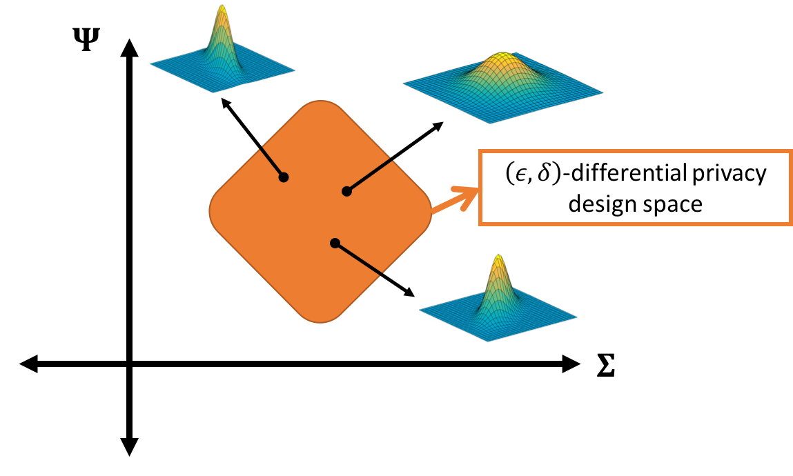
Figure 2: A conceptual display of the MVG design space. The illustration visualizes the design space coordinated by the two design parameters of $\mathcal{MVG}_{m,n}(\mathbf{0},\boldsymbol{\Sigma},\boldsymbol{\Psi})$. Each point on the space corresponds to an instance of $\mathcal{MVG}_{m,n}(\mathbf{0},\boldsymbol{\Sigma},\boldsymbol{\Psi})$. From this perspective, Theorem 2 suggests that any instance of $\mathcal{MVG}_{m,n}(\mathbf{0},\boldsymbol{\Sigma},\boldsymbol{\Psi})$ in the (conceptual) shaded area would preserve $(\epsilon,\delta)$-differential privacy.

Remark 1.

In Theorem 2, we assume that the Frobenius norm of the query function is bounded for all possible datasets by $\gamma$. This assumption is valid in practice because real-world data are rarely unbounded (cf. [69]), and it is a common assumption in the analysis of differential privacy for multi-dimensional query functions (cf. [3, 27, 70, 25]).

Remark 2.

The values of the generalized harmonic numbers – $H_{r}$, and $H_{r,1/2}$ – can be obtained from the table lookup for a given value of $r$, or can easily be computed recursively [71].

The sufficient condition in Theorem 2 yields an important observation: the privacy guarantee by the MVG mechanism depends only on the singular values of $\boldsymbol{\Sigma}$ and $\boldsymbol{\Psi}$ through their norm. In other words, we may have multiple instances of $\mathcal{MVG}_{m,n}(\mathbf{0},\boldsymbol{\Sigma},\boldsymbol{\Psi})$ that yield the exact same privacy guarantee (cf. Figure 2). This phenomenon gives rise to an interesting novel concept of directional noise, which will be discussed in Section 5.

We emphasize again that, in Theorem 2, we derive the sufficient condition for the MVG mechanism to guarantee $(\epsilon,\delta)$-differential privacy without making structural assumption about the matrix-valued query function. In the next two sections, we illustrate how incorporating the knowledge about the intrinsic structural characteristic of the matrix-valued query function of interest can yield an alternative sufficient condition. Then, we prove that such alternative sufficient condition can provide the better utility, when compared to the analysis without using the structural knowledge.

4.3 Differential Privacy Analysis for Symmetric Positive Semi-Definite (PSD) Matrix-Valued Query

To provide a concrete example of how the structural characteristics of the matrix-valued query function can be exploited via the MVG mechanism, we consider a matrix-valued query function that is symmetric positive semi-definite (PSD). To avoid being cumbersome, we will drop the explicit ’symmetric’ in the subsequent references, but the readers should keep in mind that we work with symmetric matrices here. First, let us define a positive semi-definite matrix in our context.

Definition 5.

A symmetric matrix $\mathbf{X}\in\mathbb{R}^{n\times n}$ is positive semi-definite (PSD) if $\mathbf{v}^{T}\mathbf{X}\mathbf{v}\geq 0$ for all non-zero $\mathbf{v}\in\mathbb{R}^{n}$.

Conceptually, we can think of a positive semi-definite matrix in matrix analysis as the similar notion to a non-negative number in scalar-valued analysis. More importantly, positive semi-definite matrices occur regularly in practical settings. Examples of positive semi-definite matrices in practice include the maximum likelihood estimate of the covariance matrix [62, chapter 7], the Hessian matrix [62, chapter 7], the kernel matrix in machine learning [28, 72], and the Laplacian matrix of a graph [29].

With respect to differential privacy analysis, the assumption of positive semi-definiteness on the query function is only applicable if it holds for every possible instance of the datasets. Fortunately, this is true for all of the aforementioned matrix-valued query functions because the positive semi-definiteness is the intrinsic nature of such functions. In other words, if a user queries the maximum likelihood estimate of the covariance matrix of the dataset, the (non-private) matrix-valued query answer would always be positive semi-definite regardless of the dataset from which it is computed. The same property applies to other examples given. We refer to this type of property as intrinsic to the matrix-valued query function since it holds due only to the nature of the query function regardless of the nature of the dataset. This is clearly crucial in differential privacy analysis as differential privacy considers the worst-case scenario, so any assumption made would only be valid if it applies even in such scenario.

Before presenting the main result, we emphasize that the intrinsic nature phenomenon is not unique to positive semi-definite matrix. In other words, there are many other structural properties of the matrix-valued query function that are also intrinsic. For example, the adjacency matrix for an undirected graph is always symmetric [29], and the bi-stochastic matrix always has all non-negative entries with each row and column sums up to one [32]. Therefore, the idea of exploiting structural characteristics of the matrix-valued query function is very applicable in practice under the setting of privacy-aware analysis.

Returning to the main result, we consider the MVG mechanism on a query function that is symmetric positive semi-definite. Due to the definitive symmetry of the query function output, it is reasonable to impose the design choice $\boldsymbol{\Sigma}=\boldsymbol{\Psi}$ on the MVG mechanism. The rationale is that, since the query function is symmetric, its row-wise covariance and column-wise covariance are necessarily equal if we view the query output as a random variable. Hence, it is reasonable to employ the matrix-valued noise with the same symmetry. As a result, this helps restrict our design space to that with $\boldsymbol{\Sigma}=\boldsymbol{\Psi}$. With this setting, we present the following theorem which states the sufficient condition for the MVG mechanism to preserve $(\epsilon,\delta)$-differential privacy when the query function is symmetric positive semi-definite.

Theorem 3.

Given a symmetric positive semi-definite (PSD) matrix-valued query function $f(\mathbf{X})\in\mathbb{R}^{r\times r}$, let $\boldsymbol{\sigma}(\boldsymbol{\Sigma}^{-1})=[\sigma_{1}(\boldsymbol{\Sigma}^{-1}),\ldots,\sigma_{r}(\boldsymbol{\Sigma}^{-1})]^{T}$ be the vectors of non-increasingly ordered singular values of $\boldsymbol{\Sigma}^{-1}$, let $\boldsymbol{\Psi}=\boldsymbol{\Sigma}$, and let the relevant variables be defined according to Table 1. Then, the MVG mechanism guarantees $(\epsilon,\delta)$-differential privacy if $\boldsymbol{\Sigma}$ satisfy the following condition,

$$\left\|\boldsymbol{\sigma}(\boldsymbol{\Sigma}^{-1})\right\|_{2}^{2}\leq\frac{(-\beta+\sqrt{\beta^{2}+8\omega\epsilon})^{2}}{4\omega^{2}},$$ (8)

where $\omega=4H_{r}\gamma s_{2}(f)$, and $\beta=2r{}^{1/2}\zeta(\delta)H_{r}s_{2}(f)$.

Proof.

The proof starts from the same characteristic equation (Eq. (2)) as in Theorem 2. However, since the query function is symmetric, $f(\mathbf{X})=f(\mathbf{X})^{T}$. Furthermore, since we impose $\boldsymbol{\Psi}=\boldsymbol{\Sigma}$, the characteristic equation can be simplified as,

$$\mathrm{tr}[\boldsymbol{\Sigma}^{-1}\mathcal{Y}^{T}\boldsymbol{\Sigma}^{-1}\boldsymbol{\Delta}+\boldsymbol{\Sigma}^{-1}\boldsymbol{\Delta}^{T}\boldsymbol{\Sigma}^{-1}\mathcal{Y}+\boldsymbol{\Sigma}^{-1}f(\mathbf{X}_{2})\boldsymbol{\Sigma}^{-1}f(\mathbf{X}_{2})-\boldsymbol{\Sigma}^{-1}f(\mathbf{X}_{1})\boldsymbol{\Sigma}^{-1}f(\mathbf{X}_{1})]\leq 2\epsilon.$$ (9)

Again, this condition needs to be met with probability $\geq 1-\delta$ for the MVG mechanism to preserve $(\epsilon,\delta)$-differential privacy.

First, consider the first term: $\mathrm{tr}[\boldsymbol{\Sigma}^{-1}\mathcal{Y}^{T}\boldsymbol{\Sigma}^{-1}\boldsymbol{\Delta}]$. This term is exactly the same as the first term in the proof of Theorem 2, i.e. the first term of Eq. (2). Hence, we readily have the upper bound on this term as

$$\mathrm{tr}[\boldsymbol{\Sigma}^{-1}\mathcal{Y}^{T}\boldsymbol{\Sigma}^{-1}\boldsymbol{\Delta}]\leq\gamma s_{2}(f)H_{r}\left\|\boldsymbol{\sigma}(\boldsymbol{\Sigma}^{-1})\right\|_{2}^{2}+m^{1/2}\zeta(\delta)H_{r}s_{2}(f)\left\|\boldsymbol{\sigma}(\boldsymbol{\Sigma}^{-1})\right\|_{2},$$ (10)

with probability $\geq 1-\delta$. We note two minor differences between Eq. (5) and Eq. (10). First, the factor of $(mn)^{1/4}$ becomes $m^{1/2}$. This is simply due to the fact that $n=m$ in the current setup with a PSD query function. Second, the variable $\phi=(\left\|\boldsymbol{\sigma}(\boldsymbol{\Sigma}^{-1})\right\|_{2}\left\|\boldsymbol{\sigma}(\boldsymbol{\Psi}^{-1})\right\|_{2})^{1/2}$ in Eq. (5) becomes simply $\left\|\boldsymbol{\sigma}(\boldsymbol{\Sigma}^{-1})\right\|_{2}$ in Eq. (10). This is due to the fact that $\boldsymbol{\Psi}=\boldsymbol{\Sigma}$ with the current PSD setting. Apart from these, Eq. (5) and Eq. (10) are equivalent.

Second, consider the second term: $\mathrm{tr}[\boldsymbol{\Sigma}^{-1}\boldsymbol{\Delta}^{T}\boldsymbol{\Sigma}^{-1}\mathcal{Y}]$. Again, the second term of Eq. (9) is the same as that of Eq. (2). Hence, we can readily write,

$$\mathrm{tr}[\boldsymbol{\Sigma}^{-1}\boldsymbol{\Delta}^{T}\boldsymbol{\Sigma}^{-1}\mathcal{Y}]\leq\gamma H_{r}s_{2}(f)\left\|\boldsymbol{\sigma}(\boldsymbol{\Sigma}^{-1})\right\|_{2}^{2}+m{}^{1/2}\zeta(\delta)H_{r}s_{2}(f)\left\|\boldsymbol{\sigma}(\boldsymbol{\Sigma}^{-1})\right\|_{2},$$ (11)

with probability $\geq 1-\delta$. Again, we note the same two differences between Eq. (6) and Eq. (11) as those between Eq. (5) and Eq. (10).

Next, consider the third term and fourth term combined: $\mathrm{tr}[\boldsymbol{\Sigma}^{-1}f(\mathbf{X}_{2})\boldsymbol{\Sigma}^{-1}f(\mathbf{X}_{2})-\boldsymbol{\Sigma}^{-1}f(\mathbf{X}_{1})\boldsymbol{\Sigma}^{-1}f(\mathbf{X}_{1})]$. Let us denote for a moment $\mathbf{A}=\boldsymbol{\Sigma}^{-1}f(\mathbf{X}_{2})$ and $\mathbf{B}=\boldsymbol{\Sigma}^{-1}f(\mathbf{X}_{1})$. Then, this combined term can be re-written as, $\mathrm{tr}[\mathbf{A}^{2}-\mathbf{B}^{2}]$. Next, we show that

$$\mathrm{tr}[\mathbf{A}^{2}-\mathbf{B}^{2}]=\mathrm{tr}[(\mathbf{A}-\mathbf{B})(\mathbf{A}+\mathbf{B})]$$

by starting from the right hand side and proceeding to equate it to the left hand side.

$$\mathrm{tr}([\mathbf{A}-\mathbf{B}][\mathbf{A}+\mathbf{B}])= \mathrm{tr}(\mathbf{A}\mathbf{A}+\mathbf{A}\mathbf{B}-\mathbf{B}\mathbf{A}-\mathbf{B}\mathbf{B})$$

$$= \mathrm{tr}(\mathbf{A}^{2})+\mathrm{tr}(\mathbf{A}\mathbf{B})-\mathrm{tr}(\mathbf{B}\mathbf{A})-\mathrm{tr}(\mathbf{B}^{2})$$

$$= \mathrm{tr}(\mathbf{A}^{2})+\mathrm{tr}(\mathbf{A}\mathbf{B})-\mathrm{tr}(\mathbf{A}\mathbf{B})-\mathrm{tr}(\mathbf{B}^{2})$$

$$= \mathrm{tr}(\mathbf{A}^{2})-\mathrm{tr}(\mathbf{B}^{2})$$

$$= \mathrm{tr}(\mathbf{A}^{2}-\mathbf{B}^{2}),$$

whereas the first-to-second line uses the additive property of the trace, and the second-to-third line uses the commutative property of the trace. Therefore, from this equation, we can write

$$\mathrm{tr}[\boldsymbol{\Sigma}^{-1}f(\mathbf{X}_{2})\boldsymbol{\Sigma}^{-1}f(\mathbf{X}_{2})-\boldsymbol{\Sigma}^{-1}f(\mathbf{X}_{1})\boldsymbol{\Sigma}^{-1}f(\mathbf{X}_{1})]$$

$$= \mathrm{tr}[(\boldsymbol{\Sigma}^{-1}f(\mathbf{X}_{2})-\boldsymbol{\Sigma}^{-1}f(\mathbf{X}_{1}))(\boldsymbol{\Sigma}^{-1}f(\mathbf{X}_{2})+\boldsymbol{\Sigma}^{-1}f(\mathbf{X}_{1}))]$$

$$= \mathrm{tr}[\boldsymbol{\Sigma}^{-1}(f(\mathbf{X}_{2})-f(\mathbf{X}_{1}))\boldsymbol{\Sigma}^{-1}(f(\mathbf{X}_{2})+f(\mathbf{X}_{1}))]$$

$$= \mathrm{tr}[\boldsymbol{\Sigma}^{-1}\tilde{\boldsymbol{\Delta}}\boldsymbol{\Sigma}^{-1}(f(\mathbf{X}_{2})+f(\mathbf{X}_{1}))],$$

where $\tilde{\boldsymbol{\Delta}}=-\boldsymbol{\Delta}$. Then, we can use Lemma 3 to write,

$$\mathrm{tr}[\boldsymbol{\Sigma}^{-1}\tilde{\boldsymbol{\Delta}}\boldsymbol{\Sigma}^{-1}(f(\mathbf{X}_{2})+f(\mathbf{X}_{1}))]\leq\sum_{i=1}^{r}\sigma_{i}(\boldsymbol{\Sigma}^{-1}\tilde{\boldsymbol{\Delta}})\sigma_{i}(\boldsymbol{\Sigma}^{-1}(f(\mathbf{X}_{2})+f(\mathbf{X}_{1}))).$$

Next, we use Lemma 2 to bound the two sets of singular values as follows. For the first set of singular values,

$$\sigma_{i}(\boldsymbol{\Sigma}^{-1}\tilde{\boldsymbol{\Delta}})\leq\frac{\left\|\boldsymbol{\Sigma}^{-1}\tilde{\boldsymbol{\Delta}}\right\|_{F}}{\sqrt{i}}\leq\frac{\left\|\boldsymbol{\Sigma}^{-1}\right\|_{F}\left\|\tilde{\boldsymbol{\Delta}}\right\|_{F}}{\sqrt{i}}\leq\frac{\left\|\boldsymbol{\sigma}(\boldsymbol{\Sigma}^{-1})\right\|_{2}s_{2}(f)}{\sqrt{i}},$$

whereas the last step follows from the fact that $\left\|\tilde{\boldsymbol{\Delta}}\right\|_{F}=\left\|-\boldsymbol{\Delta}\right\|_{F}=\left\|\boldsymbol{\Delta}\right\|_{F}\leq s_{2}(f)$. For the second set of singular values,

$$\sigma_{i}(\boldsymbol{\Sigma}^{-1}(f(\mathbf{X}_{2})+f(\mathbf{X}_{1}))) \leq\frac{\left\|\boldsymbol{\Sigma}^{-1}(f(\mathbf{X}_{2})+f(\mathbf{X}_{1}))\right\|_{F}}{\sqrt{i}}$$

$$\leq\frac{\left\|\boldsymbol{\Sigma}^{-1}\right\|_{F}\left\|(f(\mathbf{X}_{2})+f(\mathbf{X}_{1}))\right\|_{F}}{\sqrt{i}}$$

$$\leq\frac{\left\|\boldsymbol{\Sigma}^{-1}\right\|_{F}(\left\|f(\mathbf{X}_{2})\right\|_{F}+\left\|f(\mathbf{X}_{1})\right\|_{F})}{\sqrt{i}}$$

$$\leq\frac{\left\|\boldsymbol{\sigma}(\boldsymbol{\Sigma}^{-1})\right\|_{2}2\gamma}{\sqrt{i}},$$

whereas the second-to-third line follows from the triangular inequality. Then, we combine the two bounds on the two sets of singular values to get a bound for the third term and fourth term combined as,

$$\mathrm{tr}[\boldsymbol{\Sigma}^{-1}f(\mathbf{X}_{2})\boldsymbol{\Sigma}^{-1}f(\mathbf{X}_{2})-\boldsymbol{\Sigma}^{-1}f(\mathbf{X}_{1})\boldsymbol{\Sigma}^{-1}f(\mathbf{X}_{1})]\leq 2\gamma s_{2}(f)H_{r}\left\|\boldsymbol{\sigma}(\boldsymbol{\Sigma}^{-1})\right\|_{2}.$$

Four terms combined: by combining the four terms and rearranging them, the characteristic equation becomes,

$$\omega\left\|\boldsymbol{\sigma}(\boldsymbol{\Sigma}^{-1})\right\|_{2}^{2}+\beta\left\|\boldsymbol{\sigma}(\boldsymbol{\Sigma}^{-1})\right\|_{2}\leq 2\epsilon.$$ (12)

This is a quadratic equation, of which the solution is $\left\|\boldsymbol{\sigma}(\boldsymbol{\Sigma}^{-1})\right\|_{2}\in[\frac{-\beta-\sqrt{\beta^{2}+8\omega\epsilon}}{2\omega},\frac{-\beta+\sqrt{\beta^{2}+8\omega\epsilon}}{2\omega}]$. Since we know that $\left\|\boldsymbol{\sigma}(\boldsymbol{\Sigma}^{-1})\right\|_{2}\geq 0$ due to the axiom of the norm, we only have the one-sided solution,

$$\left\|\boldsymbol{\sigma}(\boldsymbol{\Sigma}^{-1})\right\|_{2}\leq\frac{-\beta+\sqrt{\beta^{2}+8\omega\epsilon}}{2\omega},$$

which immediately implies the criterion in Theorem 3. ∎

The sufficient condition in Theorem 3 shares the similar observation to that in Theorem 2, i.e. the privacy guarantee by the MVG mechanism with a positive semi-definite query function depends only on the singular values of $\boldsymbol{\Sigma}$ (and $\boldsymbol{\Psi}$, effectively). However, the two theorems differ slightly in that one is a function of $\alpha$, while the other is a function of $\omega$. This is clearly the result of the PSD assumption made by Theorem 3, but not by Theorem 2. In the next section, we claim that, if the matrix-valued query function of interest is positive semi-definite, it is more beneficial to apply Theorem 3 than Theorem 2 in most practical cases. This fosters the notion that exploiting the structure of the matrix-valued query function is attractive.

4.4 Comparative Analysis on the Benefit of Exploiting Structural Characteristics of Matrix-Valued Query Functions

In Section 4.2 and Section 4.3, we discuss two sufficient conditions for the MVG mechanism to guarantee $(\epsilon,\delta)$-differential privacy in Theorem 2 and Theorem 3, respectively. The two theorems differ in one significant way – Theorem 2 does not utilize the structural characteristic of the matrix-valued query function, whereas Theorem 3 does. More specifically, Theorem 3 utilizes the positive semi-definiteness of the matrix-valued query function.

In this section, we establish the claim that such utilization can be beneficial to the MVG mechanism for privacy-aware data analysis. To establish the benefit notion, we first observe that both Theorem 2 and Theorem 3 put an upper-bound on the singular values $\boldsymbol{\sigma}(\boldsymbol{\Sigma}^{-1})$ and $\boldsymbol{\sigma}(\boldsymbol{\Psi}^{-1})$. Let us consider only $\boldsymbol{\sigma}(\boldsymbol{\Sigma}^{-1})$ for the moment. It is well-known that the singular values of an inverted matrix is the inverse of the singular values, i.e. $\sigma_{i}(\boldsymbol{\Sigma}^{-1})=1/\sigma_{i}(\boldsymbol{\Sigma})$. Hence, we can write

$$\left\|\boldsymbol{\sigma}(\boldsymbol{\Sigma}^{-1})\right\|_{2}=\sqrt{\sum_{i=1}^{m}\frac{1}{\sigma_{i}^{2}(\boldsymbol{\Sigma})}}.$$ (13)

This representation of $\left\|\boldsymbol{\sigma}(\boldsymbol{\Sigma}^{-1})\right\|_{2}$ provides a very intuitive view of the sufficient conditions in Theorem 2 and Theorem 3 as follows.

In the MVG mechanism, the privacy preservation is achieved via the addition of the matrix noise. Higher level of privacy guarantee requires more perturbation. For additive noise, the notion of “more” here can be quantified by the variance of the noise. Specifically, the noise with higher variance provides more perturbation. The last connection we need to make is that between the notion of the noise variance and the singular values of the covariance $\sigma_{i}(\boldsymbol{\Sigma})$. In Section 5.2, we provide the detail of this connection. Here, it suffices to say that each singular value of the covariance matrix, $\sigma_{i}(\boldsymbol{\Sigma})$, corresponds to a component of the overall variance of the matrix-variate Gaussian noise. Therefore, intuitively, the larger the singular values are, the larger the overall variance becomes, i.e. the higher the perturbation is. However, there is clearly a tradeoff. Although higher variance can provide better privacy protection, it can also inadvertently hurt the utility of the MVG mechanism. In signal-processing terminology, this degradation of the utility can be described by the reduction in the signal-to-noise ratio (SNR) due to the increase in the perturbation level, i.e. the increase in noise variance. Hence, our notion of better MVG mechanism, and, more broadly, better mechanism for differential privacy, corresponds to that of higher SNR as follows.

Axiom 1.

A differential-private mechanism has the higher signal-to-noise ratio (SNR) if it employs the perturbation with the lower variance.

With this axiom and the given intuition about $\sigma_{i}(\boldsymbol{\Sigma})$, let us revisit Eq. (13). To achieve low noise variance, $\sigma_{i}(\boldsymbol{\Sigma})$ needs to be as low as possible. From Eq. (13), it is clear that low $\sigma_{i}(\boldsymbol{\Sigma})$ corresponds to large $\left\|\boldsymbol{\sigma}(\boldsymbol{\Sigma}^{-1})\right\|_{2}$. Hence, from Axiom 1, it is desirable to have $\left\|\boldsymbol{\sigma}(\boldsymbol{\Sigma}^{-1})\right\|_{2}$ as large as possible, while still preserving differential privacy. However, the sufficient conditions in Theorem 2 and Theorem 3 put the (different) constraints on how large $\left\|\boldsymbol{\sigma}(\boldsymbol{\Sigma}^{-1})\right\|_{2}$ can be in order to preserve $(\epsilon,\delta)$-differential privacy. Then, clearly, for fixed $(\epsilon,\delta)$, the better mechanism according to Axiom 1 is the one with the higher upper-bound on $\left\|\boldsymbol{\sigma}(\boldsymbol{\Sigma}^{-1})\right\|_{2}$. Therefore, we establish the following axiom for our comparative analysis.

Axiom 2.

For the MVG mechanism, the ($\epsilon,\delta$)-differential privacy sufficient condition with the higher SNR is the one with the larger upper-bound on $\left\|\boldsymbol{\sigma}(\boldsymbol{\Sigma}^{-1})\right\|_{2}$ and $\left\|\boldsymbol{\sigma}(\boldsymbol{\Psi}^{-1})\right\|_{2}$ for any fixed $(\epsilon,\delta)$.

Then, we can now return to the main objective of this section, i.e. to establish the benefit of exploiting structural characteristics of matrix-valued query functions. Recall that the main difference in the setup of Theorem 2 and Theorem 3 is that the former does not utilize the structural characteristic of the matrix-valued query function, while the latter utilizes the positive semi-definiteness characteristic. As a result, Theorem 2 and Theorem 3 have different sufficient conditions. More specifically, taken into the fact that $\boldsymbol{\Psi}=\boldsymbol{\Sigma}$ in the setting of Theorem 3, the two sufficient conditions only differ by the upper-bound they constrain on how large $\left\|\boldsymbol{\sigma}(\boldsymbol{\Sigma}^{-1})\right\|_{2}$ and $\left\|\boldsymbol{\sigma}(\boldsymbol{\Psi}^{-1})\right\|_{2}$ can be. Therefore, to compare the two sufficient conditions, we only need to compare their upper-bounds. The following theorem presents the main result of this comparison.

Theorem 4.

Let $f(\mathbf{X})\in\mathbb{R}^{r\times r}$ be a symmetric positive semi-definite matrix-valued query function. Then, the MVG mechanism on $f(\mathbf{X})$ implemented by Theorem 3 – which utilizes the PSD characteristic – has higher SNR than that implemented by Theorem 2 – which does not utilize the PSD characteristic, if one of the following conditions is met:

$$s_{2}(f)\leq\gamma$$ (14)

or

$$r>12.$$ (15)

Proof.

Recall that the two upper-bounds are $(-\beta+\sqrt{\beta^{2}+8\alpha\epsilon})^{2}/4\alpha^{2}$ and $(-\beta+\sqrt{\beta^{2}+8\omega\epsilon})^{2}/4\omega^{2}$ for Theorem 2 and Theorem 3, respectively. Recall also that both upper-bounds are derived from their respective quadratic equations (Eq. (7) and Eq. (12)). The proof is considerably simpler if we start from these two quadratic equations.

We first restate the two quadratic equations again here for Theorem 2 and Theorem 3, respectively:

$$\alpha\phi^{2}+\beta\phi-2\epsilon \leq 0$$ (16)

$$\omega\phi^{2}+\beta\phi-2\epsilon \leq 0.$$ (17)

Note that in the current setup, $f(\mathbf{X})\in\mathbb{R}^{r\times r}$ and $\boldsymbol{\Psi}=\boldsymbol{\Sigma}$, so $\phi=\left\|\boldsymbol{\sigma}(\boldsymbol{\Sigma}^{-1})\right\|_{2}$ in both theorems. Then, we use a lesser-known formula for finding roots of a quadratic equation, which has appeared in the Muller’s method for root-finding algorithm [73] and Vieta’s formulas for polynomial coefficient relations [74, 75].

$$\phi\in\left[\frac{4\epsilon}{\beta+\sqrt{\beta^{2}+8\alpha\epsilon}},\frac{4\epsilon}{\beta-\sqrt{\beta^{2}+8\alpha\epsilon}}\right],$$

and

$$\phi\in\left[\frac{4\epsilon}{\beta+\sqrt{\beta^{2}+8\omega\epsilon}},\frac{4\epsilon}{\beta-\sqrt{\beta^{2}+8\omega\epsilon}}\right],$$

for Eq. (16) and Eq. (17), respectively. Since we know that $\phi\geq 0$ in both cases due to the axiom of the norm, we have a one-sided solution for both as,

$$\phi\leq\frac{4\epsilon}{\beta-\sqrt{\beta^{2}+8\alpha\epsilon}},$$ (18)

and

$$\phi\leq\frac{4\epsilon}{\beta-\sqrt{\beta^{2}+8\omega\epsilon}},$$ (19)

for Eq. (16) and Eq. (17), respectively. These two solutions are particularly simple to compare since they are similar except for the term $\alpha$ and $\omega$ in the denominator. Recall from Axiom 2 that the better MVG mechanism is the one with the larger upper-bound. Hence, from Eq. (18) and Eq. (19), we want to show that,

$$\frac{4\epsilon}{\beta-\sqrt{\beta^{2}+8\omega\epsilon}}\geq\frac{4\epsilon}{\beta-\sqrt{\beta^{2}+8\alpha\epsilon}}.$$

The denominator is always positive since $\epsilon,\theta,\alpha>0$, so we can simplify this condition as follows.

$$\frac{4\epsilon}{\beta-\sqrt{\beta^{2}+8\omega\epsilon}} \geq\frac{4\epsilon}{\beta-\sqrt{\beta^{2}+8\alpha\epsilon}}$$

$$\beta-\sqrt{\beta^{2}+8\alpha\epsilon} \geq\beta-\sqrt{\beta^{2}+8\omega\epsilon}$$

$$\beta^{2}+8\alpha\epsilon \geq\beta^{2}+8\omega\epsilon$$

$$\alpha \geq\omega.$$

Substitute in the definition of $\alpha$ and $\omega$ and we have,

$$[H_{r}+H_{r,1/2}]\gamma^{2}+2H_{r}\gamma s_{2}(f) \geq 4H_{r}\gamma s_{2}(f)$$

$${}[H_{r}+H_{r,1/2}]\gamma^{2} \geq 2H_{r}\gamma s_{2}(f)$$

$${}[H_{r}+H_{r,1/2}]\gamma \geq 2H_{r}s_{2}(f).$$ (20)

From the inequality in Eq. (20), we can take two routes to ensure that this inequality is satisfied, and that gives rise to the two either-or conditions in Theorem 4. We explore each route separately next.

Route I. First, let us consider the relationship between $\gamma$ and $s_{2}(f)$ for PSD query functions, and show that, for PSD matrix-valued query functions, $s_{2}(f)\leq\sqrt{2}\gamma$. From the definition of the Frobenius norm,

$$s_{2}(f)= \sup_{d(\mathbf{X}_{1},\mathbf{X}_{2})=1}\left\|\mathbf{X}_{1}-\mathbf{X}_{2}\right\|_{F}$$

$$= \sup_{d(\mathbf{X}_{1},\mathbf{X}_{2})=1}\sqrt{\mathrm{tr}[(\mathbf{X}_{1}-\mathbf{X}_{2})(\mathbf{X}_{1}-\mathbf{X}_{2})^{T}]}$$

$$= \sup_{d(\mathbf{X}_{1},\mathbf{X}_{2})=1}\sqrt{\mathrm{tr}[\mathbf{X}_{1}\mathbf{X}_{1}^{T}-\mathbf{X}_{1}\mathbf{X}_{2}^{T}-\mathbf{X}_{2}\mathbf{X}_{1}^{T}+\mathbf{X}_{2}\mathbf{X}_{2}^{T}]}$$

$$= \sup_{d(\mathbf{X}_{1},\mathbf{X}_{2})=1}\sqrt{\mathrm{tr}[\mathbf{X}_{1}\mathbf{X}_{1}^{T}]-2\mathrm{tr}[\mathbf{X}_{1}\mathbf{X}_{2}^{T}]+\mathrm{tr}[\mathbf{X}_{2}\mathbf{X}_{2}^{T}]}$$

Since both $\mathbf{X}_{1}$ and $\mathbf{X}_{2}$ are PSD, $\mathbf{X}_{1}\mathbf{X}_{2}^{T}$ is also PSD [76]. Hence, it follows from a property of the trace and the PSD matrix that,

$$\mathrm{tr}[\mathbf{X}_{1}\mathbf{X}_{2}^{T}]=\sum\lambda_{i}(\mathbf{X}_{1}\mathbf{X}_{2}^{T})\geq 0.$$

With this fact, along with the fact that $\left\|\mathbf{X}\right\|_{F}=\sqrt{\mathrm{tr}(\mathbf{X}\mathbf{X}^{T})}\leq\gamma$, it immediately follows that,

$$s_{2}(f)\leq\sqrt{\mathrm{tr}[\mathbf{X}_{1}\mathbf{X}_{1}^{T}]+\mathrm{tr}[\mathbf{X}_{2}\mathbf{X}_{2}^{T}]}\leq\sqrt{2\gamma^{2}}=\sqrt{2}\gamma.$$

Next, let us return to the inequality in Eq. (20) and substitute in $s_{2}(f)\leq\sqrt{2}\gamma$.

$$[H_{r}+H_{r,1/2}]\gamma \geq 2\sqrt{2}H_{r}\gamma$$

$$H_{r}+H_{r,1/2} \geq 2\sqrt{2}H_{r}$$

$$H_{r,1/2} \geq(2\sqrt{2}-1)H_{r}.$$ (21)

Using the definition of the harmonic number, we can write

$$\sum_{i=1}^{r}\frac{1}{\sqrt{r}}\geq(2\sqrt{2}-1)\sum_{i=1}^{r}\frac{1}{r}.$$

Since $\frac{1}{\sqrt{r}}>\frac{1}{r}$ for all $r>1$, it is clear that this condition is met for all $r$ greater than a certain threshold. The threshold can easily be acquired numerically or analytically to be $r>12$. This completes the proof of the first route.

Route II. Second, we use the fact that $\frac{1}{\sqrt{r}}\geq\frac{1}{r}$ for $r>0$. Then, it is clear from the definition of the harmonic number that $H_{r,1/2}\geq H_{r}$. Hence, we can write the inequality in Eq. (20) as,

$$[H_{r}+H_{r,1/2}]\gamma \geq 2H_{r}s_{2}(f)$$

$$2H_{r}\gamma \geq 2H_{r}s_{2}(f)$$

$$\gamma \geq s_{2}(f),$$

which immediately completes the proof of the second route. ∎

One final necessary remark regarding this comparative analysis is to justify the practicality of the conditions in Theorem 4. We reiterate that only one of the two conditions needs to be met and discuss separately the practicality of each.

The first condition, i.e $s_{2}(f)\leq\gamma$, can be interpret conceptually as that the sensitivity should not be greater than the largest value of the query output. Two observations support the pragmatism of this condition. First, the sensitivity is derived from the change in the query output when only one input record changes. Intuitively, this suggests that such change should be confined to the largest possible value of the query output, especially for a positive semi-definite query function whose output is always non-negative. Second, one of the premises of differential privacy for statistical query is that the query can be answered accurately if the sensitivity of such query is small [3]. Hence, this condition coincides properly with the primary premise of differential privacy. To concretely illustrate its practicality, we consider two examples of matrix-valued query functions as follows.

Example 1.

Let us consider a dataset consisting of $n$ records drawn i.i.d. from an unknown $\mathbb{R}^{m}$ distribution with zero mean, and consider the covariance estimation as the query function [62, chapter 7], i.e. $f(\mathbf{X})=\frac{\mathbf{X}\mathbf{X}^{T}}{n}$. Let us assume without the loss of generality that $\mathbf{X}\in[-c,c]^{m\times n}$. Then, the largest query output value can be computed as,

$$\gamma=\sup_{\mathbf{X}}\left\|\frac{\mathbf{X}\mathbf{X}^{T}}{n}\right\|_{F}=\sup_{\mathbf{X}}\left\|\frac{1}{n}\sum_{i=1}^{n}\mathbf{x}_{i}\mathbf{x}_{i}^{T}\right\|_{F}=mc^{2}.$$

Next, the sensitivity can be computed by considering that $f(\mathbf{X})=\frac{1}{n}\mathbf{X}\mathbf{X}^{T}=\frac{1}{n}\sum_{i=1}^{n}\mathbf{x}_{i}\mathbf{x}_{i}^{T}$. Hence, for neighboring datasets $\mathbf{X}$ and $\mathbf{X}^{\prime}$, the query outputs differ by only one summand and the sensitivity can be computed as,

$$s_{2}(f)=\sup_{\mathbf{X},\mathbf{X}^{\prime}}\frac{\left\|\mathbf{x}_{j}\mathbf{x}_{j}^{T}-\mathbf{x}_{j}^{\prime}\mathbf{x}_{j}^{\prime T}\right\|_{F}}{n}\leq\frac{2\sqrt{\sum_{j=1}^{m^{2}}x_{j}(i)^{4}}}{n}=\frac{2mc^{2}}{n}.$$

Clearly, $s_{2}(f)\ll\gamma$ for any reasonably-sized dataset.

Example 2.

Let us consider the kernel matrix often used in machine learning [28, 72]. Given a kernel function $k(\mathbf{x}_{i},\mathbf{x}_{j})\in\mathbb{R}$, the kernel matrix query is $f(\mathbf{X})=\mathbf{G}\in\mathbb{R}^{n\times n}$, where $[\mathbf{G}]_{ij}=k(\mathbf{x}_{i},\mathbf{x}_{j})$. We note that the notation $[\cdot]_{ij}$ indicates the $[i^{th},j^{th}]$-element of the matrix. Let us assume further without the loss of generality that $k(\mathbf{x}_{i},\mathbf{x}_{j})\leq c$. Then, the largest query output value can be computed as,

$$\gamma=\sup_{\mathbf{X}}\left\|\mathbf{G}\right\|_{F}=\sup\sqrt{\sum_{i,j}k(\mathbf{x}_{i},\mathbf{x}_{j})^{2}}=nc.$$

Next, the sensitivity can be computed by considering that the $[i^{th},j^{th}]$-element of the matrix $\mathbf{G}$ only depends on $\mathbf{x}_{i},\mathbf{x}_{j}\in\mathbf{X}$, but not on any other record. Hence, for neighboring datasets $\mathbf{X}$ and $\mathbf{X}^{\prime}$, the query outputs differ by only one row and column. Then, the sensitivity can be computed as,

$$s_{2}(f)=\sup_{\mathbf{X},\mathbf{X}^{\prime}}\left\|\mathbf{G}-\mathbf{G}^{\prime}\right\|_{F}=\sup\sqrt{2\sum_{i=1}^{n}4k(\mathbf{x}_{k},\mathbf{x}_{i})^{2}-4k(\mathbf{x}_{k},\mathbf{x}_{k})^{2}}=c\sqrt{8n-4}.$$

From the values of $\gamma$ and $s_{2}(f)$, it can easily be shown that $s_{2}(f)<\gamma$ for $n>7$. For the kernel matrix used in machine learning, $n$ corresponds to the number of samples in the dataset. Clearly, in practice, the dataset has considerably more than 7 samples, so this condition is always met for the kernel matrix query function.

Next, let us consider the second condition, i.e. $r>12$, which simply states that the dimension of the positive semi-definite matrix-valued query function should be larger than 12. This can be justified simply by noting that many real-world positive semi-definite matrix-valued query functions have dimensions significantly larger than 12. For example, as seen in Example 1 and Example 2, the dimensions of the covariance matrix and the kernel matrix depend on the number of features and data samples, respectively. Both quantities are generally considerably larger than 12 in practice. Similarly, the Laplacian matrix of a graph has its dimension depending upon the number of nodes in the graph, which is usually considerably larger than 12 [29].

Finally, we emphasize that only one of the two conditions, i.e. $s_{2}(f)\leq\gamma$ or $r>12$, needs to be satisfied in order for the MVG mechanism to fully exploit the positive semi-definiteness characteristic of the matrix-valued query function. As we have shown, this poses little restriction in practice.

As a segue to the next section, we revisit the sufficient conditions for the MVG mechanism to guarantee ($\epsilon,\delta$)-differential privacy in Theorem 2 and Theorem 3. In both theorems, the sufficient conditions put an upper-bound only on the singular values of the two covariance matrices $\boldsymbol{\Sigma}$ and $\boldsymbol{\Psi}$. We briefly describe in this section that each singular value can be interpret as a variance of the noise. In the next section, we provide a detailed analysis on this interpretation and how it can be exploited for the application of privacy-aware data analysis with the MVG mechanism.

5 Directional Noise for Matrix-Valued Query

Recall from the differential privacy analysis of the MVG mechanism (Theorem 2 and Theorem 3) that the sufficient conditions for the MVG mechanism to guarantee $(\epsilon,\delta)$-differential privacy in both theorems only apply to the singular values of the two covariance matrices $\boldsymbol{\Sigma}$ and $\boldsymbol{\Psi}$. Here, we investigate the ramification of this result via the novel notion of directional noise.

5.1 Motivation for Non-i.i.d. Noise for Matrix-Valued Query

For a matrix-valued query function, the standard method for basic mechanisms that use additive noise is by adding the independent and identically distributed (i.i.d.) noise to each element of the matrix query. However, as common in matrix analysis [62], the matrices involved often have some geometric and algebraic characteristics that can be exploited. As a result, it is usually the case that only certain “parts” – the term which will be defined more precisely shortly – of the matrices contain useful information. In fact, this is one of the rationales behind many compression techniques such as the popular principal component analysis (PCA) [28, 77, 78]. Due to this reason, adding the same amount of noise to every “part” of the matrix query may be highly suboptimal.

5.2 Directional Noise as a Non-i.i.d. Noise

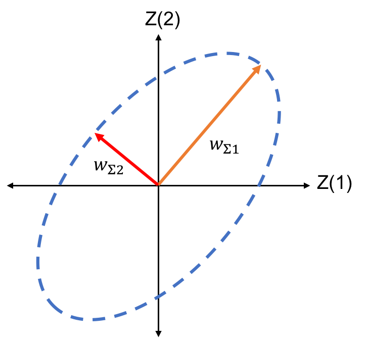
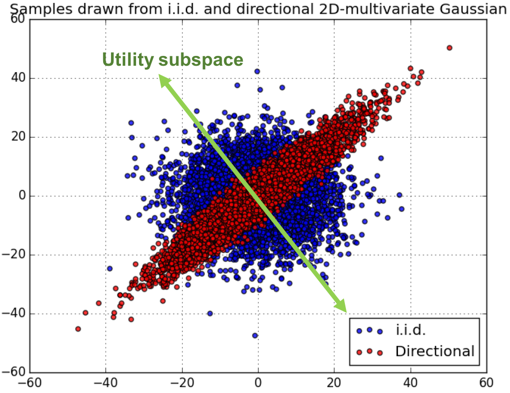
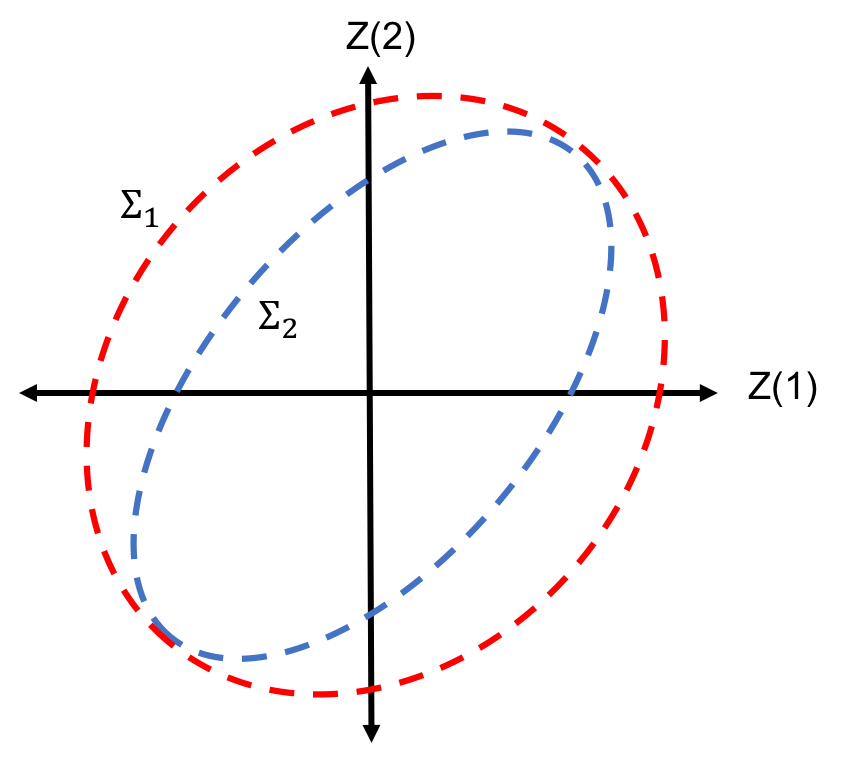
Figure 3: (Left) An ellipsoid of equi-density contour of a 2D multivariate Gaussian distribution. The blue contour represents every point in this 2D space which has the same probability density under this distribution. The two arrows indicate the principal axes of this ellipsoid. (Middle) Directional noise (red) and i.i.d. noise (blue) drawn from a 2D-multivariate Gaussian distribution. The green line represents a possible utility subspace that can benefit from this instance of directional noise. (Right) Graphical comparison of the noise generated from two different values of $\boldsymbol{\Sigma}$. The dash ellipsoids represent the equi-density contours corresponding to the noise generated by the two different values of $\boldsymbol{\Sigma}$. Clearly, from the signal-to-noise ratio (SNR) point of view, the blue contour ($\boldsymbol{\Sigma}_{2}$) is more preferable to the red contour ($\boldsymbol{\Sigma}_{1}$) since its noise has smaller overall variance.

Let us elaborate further on the “parts” of a matrix. In matrix analysis, the prevalent paradigm to extract underlying properties of a matrix is via matrix factorization [62]. This is a family of algorithms and the specific choice depends upon the application and types of insights it requires. Particularly, in our application, the factorization that is informative is the singular value decomposition (SVD) (Theorem 1) of the two covariance matrices of $\mathcal{MVG}_{m,n}(\mathbf{0},\boldsymbol{\Sigma},\boldsymbol{\Psi})$.

Consider first the covariance matrix $\boldsymbol{\Sigma}\in\mathbb{R}^{m\times m}$, and write its SVD as, $\boldsymbol{\Sigma}=\mathbf{W}_{1}\boldsymbol{\Lambda}\mathbf{W}_{2}^{T}$. It is well-known that, for the covariance matrix, we have the equality $\mathbf{W}_{1}=\mathbf{W}_{2}$ since it is positive definite (cf. [79, 62]). Hence, let us more concisely write the SVD of $\boldsymbol{\Sigma}$ as,

$$\boldsymbol{\Sigma}=\mathbf{W}_{\boldsymbol{\Sigma}}\boldsymbol{\Lambda}_{\boldsymbol{\Sigma}}\mathbf{W}_{\boldsymbol{\Sigma}}^{T}.$$

This representation gives us a very useful insight to the noise generated from $\mathcal{MVG}_{m,n}(\mathbf{0},\boldsymbol{\Sigma},\boldsymbol{\Psi})$: it tells us the directions of the noise via the column vectors of $\mathbf{W}_{\boldsymbol{\Sigma}}$, and variance of the noise in each direction via the singular values in $\boldsymbol{\Lambda}_{\boldsymbol{\Sigma}}$.

For simplicity, let us consider a two-dimensional multivariate Gaussian distribution, i.e. $m=2$, so there are two column vectors of $\mathbf{W}_{\boldsymbol{\Sigma}}=[\mathbf{w}_{\boldsymbol{\Sigma}1},\mathbf{w}_{\boldsymbol{\Sigma}2}]$. The geometry of this distribution can be depicted by an ellipsoid, e.g. the dash contour in Figure 3, Left (cf. [77, ch. 4], [78, ch. 2]). This ellipsoid is characterized by its two principal axes – the major and the minor axes. It is well-known that the two column vectors from SVD, i.e. $\mathbf{w}_{\boldsymbol{\Sigma}1}$ and $\mathbf{w}_{\boldsymbol{\Sigma}2}$, are unit vectors pointing in the directions of the major and minor axes of this ellipsoid, and more importantly, the length of each axis is characterized by its corresponding singular value, i.e. $\sigma_{\boldsymbol{\Sigma}1}$ and $\sigma_{\boldsymbol{\Sigma}2}$, respectively (cf. [77, ch. 4]) (recall from Theorem 1 that $diag(\boldsymbol{\Lambda}_{\boldsymbol{\Sigma}})=[\sigma_{\boldsymbol{\Sigma}1},\sigma_{\boldsymbol{\Sigma}2}]$). This is illustrated by Figure 3, Left. Therefore, when we consider the noise generated from this 2D multivariate Gaussian distribution, we arrive at the following interpretation of the SVD of its covariance matrix: the noise is distributed toward the two principal directions specified by $\mathbf{w}_{\boldsymbol{\Sigma}1}$ and $\mathbf{w}_{\boldsymbol{\Sigma}2}$, with the variance scaled by the corresponding singular values, $\sigma_{\boldsymbol{\Sigma}1}$ and $\sigma_{\boldsymbol{\Sigma}2}$.

We can extend this interpretation to a more general case with $m>2$, and also to the other covariance matrix $\boldsymbol{\Psi}$. Then, we have a full interpretation of $\mathcal{MVG}_{m,n}(\mathbf{0},\boldsymbol{\Sigma},\boldsymbol{\Psi})$ as follows. The matrix-valued noise distributed according to $\mathcal{MVG}_{m,n}(\mathbf{0},\boldsymbol{\Sigma},\boldsymbol{\Psi})$ has two components: the row-wise noise, and the column-wise noise. The row-wise noise and the column-wise noise are characterized by the two covariance matrices, $\boldsymbol{\Sigma}$ and $\boldsymbol{\Psi}$, respectively, as follows.

5.2.1 For the row-wise noise

• The row-wise noise is characterized by $\boldsymbol{\Sigma}$.

• SVD of $\boldsymbol{\Sigma}=\mathbf{W}_{\boldsymbol{\Sigma}}\boldsymbol{\Lambda}_{\boldsymbol{\Sigma}}\mathbf{W}_{\boldsymbol{\Sigma}}^{T}$ decomposes the row-wise noise into two components – the directions and the variances of the noise in those directions.

• The directions of the row-wise noise are specified by the column vectors of $\mathbf{W}_{\boldsymbol{\Sigma}}$.

• The variance of each row-wise-noise direction is indicated by its corresponding singular value in $\boldsymbol{\Lambda}_{\boldsymbol{\Sigma}}$.

5.2.2 For the column-wise noise

• The column-wise noise is characterized by $\boldsymbol{\Psi}$.

• SVD of $\boldsymbol{\Psi}=\mathbf{W}_{\boldsymbol{\Psi}}\boldsymbol{\Lambda}_{\boldsymbol{\Psi}}\mathbf{W}_{\boldsymbol{\Psi}}^{T}$ decomposes the column-wise noise into two components – the directions and the variances of the noise in those directions.

• The directions of the column-wise noise are specified by the column vectors of $\mathbf{W}_{\boldsymbol{\Psi}}$.

• The variance of each column-wise-noise direction is indicated by its corresponding singular value in $\boldsymbol{\Lambda}_{\boldsymbol{\Psi}}$.

Since $\mathcal{MVG}_{m,n}(\mathbf{0},\boldsymbol{\Sigma},\boldsymbol{\Psi})$ is fully characterized by its covariances, these two components of the matrix-valued noise drawn from $\mathcal{MVG}_{m,n}(\mathbf{0},\boldsymbol{\Sigma},\boldsymbol{\Psi})$ provide a complete interpretation of the matrix-variate Gaussian noise.

5.3 Directional Noise via the MVG Mechanism

With the notion of directional noise, we now revisit Theorem 2 and Theorem 3. Recall that the sufficient conditions for the MVG mechanism to preserve $(\epsilon,\delta)$-differential privacy according to both theorems put the constraint only on the singular values of $\boldsymbol{\Sigma}$ and $\boldsymbol{\Psi}$. However, as we discuss in the previous section, the singular values of $\boldsymbol{\Sigma}$ and $\boldsymbol{\Psi}$ only indicate the variance of the noise in each direction, but not the directions they are attributed to. In other words, Theorem 2 and Theorem 3 suggest that the MVG mechanism preserves $(\epsilon,\delta)$-differential privacy as long as the overall variances of the noise satisfy a certain threshold, but these variances can be attributed non-uniformly in any direction.

This major claim certainly warrants further discussion, and we will defer it to Section 6, where we present the technical detail on how to actually implement this concept of directional noise in practical settings. It is important to only note here that this claim does not mean that we can avoid adding noise in any particular direction altogether. On the contrary, there is still a minimum amount of noise required in every direction for the MVG mechanism to guarantee differential privacy, but the noise simply can be attributed unevenly in different directions (cf. Fig. 3, Right, for an example).

Finally, with the understanding of directional noise via the MVG mechanism, we can revisit the discussion in Sec. 4.4. Conceptually, the sufficient conditions in Theorem 2 and Theorem 3 impose a threshold on the minimum overall variance of the noise in every direction. Therefore, intuitively, to achieve the most utility out of the noisy query output, we want the threshold to be as low as possible (cf. Figure 3, Right). As discussed in Section 4.4, since both sufficient conditions put the constraint upon the inverse of the variance, this means that we want the upper-bound of the sufficient conditions to be as large as possible for maximum utility, and, hence, the derivation of Theorem 4.

5.4 Utility Gain via Directional Noise

As the concept of the directional noise is established, one important remaining question is how we can exploit this to enhance the utility of differential privacy. The answer to this question depends on the query function. Here, we present examples for two popular matrix-valued query functions: the identity query and the covariance matrix.

5.4.1 Identity Query

Formally, the identity query is $f(\mathbf{X})=\mathbf{X}$. We illustrate how to exploit directional noise for enhancing utility via the following two examples.

Example 3.

Consider the personalized warfarin dosing problem [80], which can be considered as the regression problem with the identity query. In the i.i.d. noise scheme, every feature used in the warfarin dosing prediction is equally perturbed. However, domain experts may have prior knowledge that some features are more critical than the others, so adding directional noise designed such that the more critical features are perturbed less can potentially yield better prediction performance.

We note from this example that the directions chosen here are among the standard basis, e.g. $\mathbf{e}_{1}=[1,0,\ldots,0]^{T},\mathbf{e}_{2}=[0,1,\ldots,0]^{T}$, which is one of the simplest forms of directions. Moreover, the directions in this example are decided based on the domain expertise. When domain knowledge is unavailable, we may still identify the useful directions by spending a fraction of the privacy budget on deriving the directions.

Example 4.

Consider again the warfarin dosing problem [80], and assume that we do not possess any prior knowledge about the predictive features. We can still learn this information from the data by spending a small privacy budget on deriving differentially-private principal components (P.C.) from available differentially-private PCA algorithms [52, 25, 27, 42, 26, 81, 82]. Each P.C. can then serve as a direction and, with directional noise, we can selectively add less noise in the highly informative directions as indicated by PCA.

As opposed to the previous example, the directions in this example are not necessary among the standard basis, but can be any unit vector. Nevertheless, this example illustrates how directional noise can provide additional utility benefit even with no assumption on the prior knowledge.

Figure 3, Middle, illustrates an example of how directional noise can provide the utility gain over i.i.d. noise. In the illustration, we assume the data with two features, and assume that we have obtained the utility direction, e.g. from PCA, represented by the green line. This can be considered as the utility subspace we desire to be least perturbed. The many small circles in the illustration represent how the i.i.d. noise and directional noise are distributed under the 2D multivariate Gaussian distribution. Clearly, directional noise can reduce the perturbation experienced on the utility subspace when compared to the i.i.d. noise.

5.4.2 Covariance Matrix

Let us consider a slightly more involved matrix-valued query similar to Example 1: the covariance matrix, i.e. $f(\mathbf{X})=\frac{1}{n}\mathbf{X}\mathbf{X}^{T}$. Here, we consider the dataset with $n$ samples and $m$ features. The following example illustrates how we can utilize directional noise for this query function.

Example 5.

Consider the Netflix prize dataset [83, 84]. A popular method for solving the Netflix challenge is via the low-rank approximation [85]. One way to perform this method is to query the covariance matrix of the dataset [26, 86, 27]. Suppose we use output perturbation to preserve differential privacy, i.e. $\mathcal{A}(f(\mathbf{X}))=f(\mathbf{X})+\mathcal{Z}$, and suppose we have prior knowledge from domain experts that some features are more informative than the others. Since the covariance matrix has the underlying property that each row and column correspond to a single feature [77], we can use this prior knowledge with directional noise by adding less noise to the rows and columns corresponding to the informative features.

This example emphasizes the usefulness of the concept of directional noise even when the query function is more complex than the simple identity query.

In the recent three examples, we derive the directions for the noise either from PCA or prior knowledge. PCA, however, is probably only suitable to the data-release type of query, e.g. the identity query. It is, therefore, still unclear how to derive the directions of the noise for a general matrix-valued query function when prior knowledge may not be available. We discuss a possible solution to this problem in the next section.

5.4.3 Directional Noise for General Matrix-Valued Query

For a general matrix-valued query function, one general possible approach to derive the directions of the noise is to use the SVD. As discussed in Section 5, SVD can decompose a matrix into its directions and variances. Hence, for a general matrix-valued query function, we can cast aside a small portion of privacy budget to derive the directions from the SVD of the query function. Clearly, the direction-derivation process via SVD needs to be private. Fortunately, there have been many works on differentially-private SVD [81, 82, 26]. We experimentally demonstrate the feasibility of the approach in Section 9.

In the next section, we discuss how we implement directional noise with the MVG mechanism in practice and propose two simple algorithms for two types of directional noise.

6 Practical Implementation of MVG Mechanism

The differential privacy condition in Theorem 2 and Theorem 3, even along with the notion of directional noise in the previous section, still leads to a large design space for the MVG mechanism. In this section, we present two simple algorithms to implement the MVG mechanism with two types of directional noise that can be appropriate for a wide range of real-world applications. Then, we conclude the section with a discussion on the sampling algorithms for $\mathcal{MVG}_{m,n}(\mathbf{0},\boldsymbol{\Sigma},\boldsymbol{\Psi})$ necessary for the practical implementation of our mechanism.

As discussed in Section 5.3, Theorem 2 and Theorem 3 state that the MVG mechanism satisfies $(\epsilon,\delta)$-differential privacy as long as the singular values of the row-wise and column-wise covariance matrices satisfy the sufficient condition. This provides tremendous flexibility in the choice of the directions of the noise. First, we notice from the sufficient condition in Theorem 2 that the singular values for $\boldsymbol{\Sigma}$ and $\boldsymbol{\Psi}$ are decoupled, i.e. they can be designed independently, whereas Theorem 3 explicitly imposes $\boldsymbol{\Psi}=\boldsymbol{\Sigma}$. Hence, the row-wise noise and column-wise noise can be considered as the two modes of noise in the MVG mechanism. By this terminology, we discuss two types of directional noise: the unimodal and equi-modal directional noise.

6.1 Unimodal Directional Noise

For the unimodal directional noise, we select one mode of the noise to be directional noise, whereas the other mode of the noise is set to be i.i.d. For this discussion, we assume that the row-wise noise is directional noise, while the column-wise noise is i.i.d. However, the opposite case can be readily analyzed with the similar analysis. Furthermore, for simplicity, we only consider the differential privacy guarantee provided by Theorem 2 for the unimodal directional noise.

We note that, apart from simplifying the practical implementation that we will discuss shortly, this type of directional noise can be appropriate for many applications. For example, for the identity query, we may not possess any prior knowledge on the quality of each sample, so the best strategy would be to consider the i.i.d. column-wise noise (recall that in our notation, samples are the column vectors).

Formally, the unimodal directional noise sets $\boldsymbol{\Psi}=\mathbf{I}_{n}$, where $\mathbf{I}_{n}$ is the $n\times n$ identity matrix. This, consequently, reduces the design space for the MVG mechanism with directional noise to only the design of $\boldsymbol{\Sigma}$. Next, consider the left side of the sufficient condition in Theorem 2, and we have

$$\left\|\boldsymbol{\sigma}(\boldsymbol{\Sigma}^{-1})\right\|_{2}=\sqrt{\sum_{i=1}^{m}\frac{1}{\sigma_{i}^{2}(\boldsymbol{\Sigma})}}\ \textrm{, and}\ \left\|\boldsymbol{\sigma}(\boldsymbol{\Psi}^{-1})\right\|_{2}=\sqrt{n}.$$ (22)

If we square both sides of the sufficient condition and re-arrange it, we get a form of the condition such that the row-wise noise in each direction is completely decoupled:

$$\sum_{i=1}^{m}\frac{1}{\sigma_{i}^{2}(\boldsymbol{\Sigma})}\leq\frac{1}{n}\frac{(-\beta+\sqrt{\beta^{2}+8\alpha\epsilon})^{4}}{16\alpha^{4}}.$$ (23)

This form gives a very intuitive interpretation of the directional noise. First, we note that, to have small noise in the $i^{th}$ direction, $\sigma_{i}(\boldsymbol{\Sigma})$ has to be small (cf. Section 5.2). However, the sum of $1/\sigma_{i}^{2}(\boldsymbol{\Sigma})$ of the noise in all directions, which should hence be large, is limited by the quantity on the right side of Eq. (23). This, in fact, explains why even with directional noise, we still need to add noise in every direction to guarantee differential privacy. Consider the case when we set the noise in one direction to be zero, and we have $\underset{\sigma\rightarrow 0}{\lim}\frac{1}{\sigma}=\infty$, which immediately violates the sufficient condition in Eq. (23).

From Eq. (23), the quantity $1/\sigma_{i}^{2}(\boldsymbol{\Sigma})$ is the inverse of the variance of the noise in the $i^{th}$ direction, so we may think of it as the precision measure of the query answer in that direction. The intuition is that the higher this value is, the lower the noise added in that direction, and, hence, the more precise the query value in that direction is. From this description, the constraint in Eq. (23) can be aptly named as the precision budget, and we immediately have the following theorem.

Theorem 5.

For the MVG mechanism with $\boldsymbol{\Psi}=\mathbf{I}_{n}$, the precision budget is $(-\beta+\sqrt{\beta^{2}+8\alpha\epsilon})^{4}/(16\alpha^{4}n)$.

Finally, the remaining task is to determine the directions of the noise and form $\boldsymbol{\Sigma}$ accordingly. To do so systematically, we first decompose $\boldsymbol{\Sigma}$ by SVD as,

$$\boldsymbol{\Sigma}=\mathbf{W}_{\boldsymbol{\Sigma}}\boldsymbol{\Lambda}_{\boldsymbol{\Sigma}}\mathbf{W}_{\boldsymbol{\Sigma}}^{T}.$$

This decomposition represents $\boldsymbol{\Sigma}$ by two components – the directions of the row-wise noise indicated by $\mathbf{W}_{\boldsymbol{\Sigma}}$, and the variance of the noise indicated by $\boldsymbol{\Lambda}_{\boldsymbol{\Sigma}}$. Since the precision budget only puts constraint upon $\boldsymbol{\Lambda}_{\boldsymbol{\Sigma}}$, this decomposition allows us to freely chose any unitary matrix for $\mathbf{W}_{\boldsymbol{\Sigma}}$ such that each column of $\mathbf{W}_{\boldsymbol{\Sigma}}$ indicates each independent direction of the noise.

Therefore, we present the following simple approach to design the MVG mechanism with the unimodal directional noise: under a given precision budget, allocate more precision to the directions of more importance.

Algorithm 1 formalizes this procedure. It takes as inputs, among other parameters, the precision allocation strategy $\boldsymbol{\theta}\in(0,1)^{m}$, and the directions $\mathbf{W}_{\boldsymbol{\Sigma}}\in\mathbb{R}^{m\times m}$. The precision allocation strategy is a vector of size $m$, whose elements, $\theta_{i}\in(0,1)$, corresponds to the importance of the $i^{th}$ direction indicated by the $i^{th}$ orthonormal column vector of $\mathbf{W}_{\boldsymbol{\Sigma}}$. The higher the value of $\theta_{i}$, the more important the $i^{th}$ direction is. Moreover, the algorithm enforces that $\sum_{i=1}^{m}\theta_{i}\leq 1$ to ensure that we do not overspend the precision budget. The algorithm, then, proceeds as follows. First, compute $\alpha$ and $\beta$ and, then, the precision budget $P$. Second, assign precision to each direction based on the precision allocation strategy. Third, derive the variance of the noise in each direction accordingly. Then, compute $\boldsymbol{\Sigma}$ from the noise variance and directions, and draw a matrix-valued noise from $\mathcal{MVG}_{m,n}(\mathbf{0},\boldsymbol{\Sigma},\mathbf{I})$. Finally, output the query answer with additive matrix noise.

We make a remark here about choosing directions of the noise. As discussed in Section 5, any orthonormal set of vectors can be used as the directions. The simplest instance of such set is the the standard basis vectors, e.g. $\mathbf{e}_{1}=[1,0,0]^{T},\mathbf{e}_{2}=[0,1,0]^{T},\mathbf{e}_{3}=[0,0,1]^{T}$ for $\mathbb{R}^{3}$.

Input: (a) privacy parameters: $\epsilon,\delta$; (b) the query function and its sensitivity: $f(\mathbf{X})\in\mathbb{R}^{m\times n},s_{2}(f)$; (c) the precision allocation strategy $\boldsymbol{\theta}\in(0,1)^{m}:\left|\boldsymbol{\theta}\right|_{1}=1$; and (d) the $m$ directions of the row-wise noise $\mathbf{W}_{\boldsymbol{\Sigma}}\in\mathbb{R}^{m\times m}$.

1. Compute $\alpha$ and $\beta$ (cf. Theorem 2).

2. Compute the precision budget $P=\frac{(-\beta+\sqrt{\beta^{2}+8\alpha\epsilon})^{4}}{16\alpha^{4}n}$.

3. for $i=1,\ldots,m$:

   1. Set $p_{i}=\theta_{i}P$.

   2. Compute the $i^{th}$ direction’s variance, $\sigma_{i}(\boldsymbol{\Sigma})=1/\sqrt{p_{i}}$.

4. Form the diagonal matrix $\boldsymbol{\Lambda}_{\boldsymbol{\Sigma}}=diag([\sigma_{1}(\boldsymbol{\Sigma}),\ldots,\sigma_{m}(\boldsymbol{\Sigma})])$.

5. Derive the covariance matrix: $\boldsymbol{\Sigma}=\mathbf{W}_{\boldsymbol{\Sigma}}\boldsymbol{\Lambda}_{\boldsymbol{\Sigma}}\mathbf{W}_{\boldsymbol{\Sigma}}^{T}$.

6. Draw a matrix-valued noise $\mathbf{Z}$ from $\mathcal{MVG}_{m,n}(\mathbf{0},\boldsymbol{\Sigma},\mathbf{I})$.

Output: $f(\mathbf{X})+\mathbf{Z}$.

Algorithm 1 MVG mechanism with unimodal directional noise.

6.2 Equi-Modal Directional Noise

Next, we consider the type of directional noise of which the row-wise noise and column-wise noise are distributed identically, which we call the equi-modal directional noise. We recommend this type of directional noise for a symmetric query function, i.e. $f(\mathbf{X})=f(\mathbf{X})^{T}\in\mathbb{R}^{m\times m}$. This covers a wide-range of query functions including the covariance matrix [25, 26, 27], the kernel matrix [28], the adjacency matrix of an undirected graph [29], and the Laplacian matrix [29]. The motivation for this recommendation is that, for symmetric query functions, any prior information about the rows would similarly apply to the columns, so it is reasonable to use identical row-wise and column-wise noise. Since Theorem 3 considers the symmetric positive semi-definite matrix-valued query function, the equi-modal directional noise can be used with both Theorem 2 and Theorem 3. However, we note that to use the equi-modal directional noise with Theorem 3, the matrix-valued query function also has to be positive semi-definite.

Formally, this type of directional noise imposes that $\boldsymbol{\Psi}=\boldsymbol{\Sigma}$. Following a similar derivation to the unimodal type, we have the following precision budget.

Theorem 6.

For the MVG mechanism with $\boldsymbol{\Psi}=\boldsymbol{\Sigma}$, the precision budget is $(-\beta+\sqrt{\beta^{2}+8\alpha\epsilon})^{2}/(4\alpha^{2})$ with Theorem 2, or $(-\beta+\sqrt{\beta^{2}+8\omega\epsilon})^{2}/(4\omega^{2})$ with Theorem 3.

We emphasize again that the choice between applying Theorem 2 or Theorem 3 for the precision budget depends on the particular query function, as discussed in Sec. 4.4. Then, following a similar procedure to the unimodal type, we present Algorithm 2 for the MVG mechanism with the equi-modal directional noise. The algorithm follows the same steps as Algorithm 1, except it derives the precision budget from Theorem 6, and draws the noise from $\mathcal{MVG}_{m,m}(\mathbf{0},\boldsymbol{\Sigma},\boldsymbol{\Sigma})$.

Input: (a) privacy parameters: $\epsilon,\delta$; (b) the query function and its sensitivity: $f(\mathbf{X})\in\mathbb{R}^{m\times m},s_{2}(f)$; (c) the precision allocation strategy $\boldsymbol{\theta}\in(0,1)^{m}:\left|\boldsymbol{\theta}\right|_{1}=1$; and (d) the $m$ noise directions $\mathbf{W}_{\boldsymbol{\Sigma}}\in\mathbb{R}^{m\times m}$.

1. Compute $\alpha$ and $\beta$ (cf. Theorem 2), or $\omega$ and $\beta$ (cf. Theorem 3) depending on the query function (cf. Section 4.4).

2. Compute the precision budget $P=\frac{(-\beta+\sqrt{\beta^{2}+8\alpha\epsilon})^{2}}{4\alpha^{2}}$ or $P=\frac{(-\beta+\sqrt{\beta^{2}+8\omega\epsilon})^{2}}{4\omega^{2}}$, according to the choice in step 1.

3. for $i=1,\ldots,m$:

   1. Set $p_{i}=\theta_{i}P$.

   2. Compute the the $i^{th}$ direction’s variance, $\sigma_{i}(\boldsymbol{\Sigma})=1/\sqrt{p_{i}}$.

4. Form the diagonal matrix $\boldsymbol{\Lambda}_{\boldsymbol{\Sigma}}=diag([\sigma_{1}(\boldsymbol{\Sigma}),\ldots,\sigma_{m}(\boldsymbol{\Sigma})])$.

5. Derive the covariance matrix: $\boldsymbol{\Sigma}=\mathbf{W}_{\boldsymbol{\Sigma}}\boldsymbol{\Lambda}_{\boldsymbol{\Sigma}}\mathbf{W}_{\boldsymbol{\Sigma}}^{T}$.

6. Draw a matrix-valued noise $\mathbf{Z}$ from $\mathcal{MVG}_{m,m}(\mathbf{0},\boldsymbol{\Sigma},\boldsymbol{\Sigma})$.

Output: $f(\mathbf{X})+\mathbf{Z}$.

Algorithm 2 MVG mechanism with equi-modal directional noise.

6.3 Sampling from $\mathcal{MVG}_{m,n}(\mathbf{0},\boldsymbol{\Sigma},\boldsymbol{\Psi})$

One remaining question on the practical implementation of the MVG mechanism is how to efficiently draw the noise from $\mathcal{MVG}_{m,n}(\mathbf{0},\boldsymbol{\Sigma},\boldsymbol{\Psi})$. Here, we present two methods to implement the $\mathcal{MVG}_{m,n}(\mathbf{0},\boldsymbol{\Sigma},\boldsymbol{\Psi})$ samplers from currently available samplers of other distributions. The first is based on the equivalence between $\mathcal{MVG}_{m,n}(\mathbf{0},\boldsymbol{\Sigma},\boldsymbol{\Psi})$ and the multivariate Gaussian distribution, and the second is based on the affine transformation of the i.i.d. normal distribution.

6.3.1 Sampling via the Multivariate Gaussian

This method uses the equivalence between $\mathcal{MVG}_{m,n}(\mathbf{0},\boldsymbol{\Sigma},\boldsymbol{\Psi})$ and the multivariate Gaussian distribution via the vectorization operator $vec(\cdot)$, and the Kronecker product $\otimes$ [62]. The relationship is described by the following lemma [59, 56, 61].

Lemma 6.

$\mathcal{X}\sim\mathcal{MVG}_{m,n}(\mathbf{M},\boldsymbol{\Sigma},\boldsymbol{\Psi})$ if and only if $vec(\mathcal{X})\sim\mathcal{N}_{mn}(vec(\mathbf{M}),\boldsymbol{\Psi}\otimes\boldsymbol{\Sigma})$, where $\mathcal{N}_{mn}(vec(\mathbf{M}),\boldsymbol{\Psi}\otimes\boldsymbol{\Sigma})$ denotes the $mn$-dimensional multivariate Gaussian distribution with mean $vec(\mathbf{M})$ and covariance $\boldsymbol{\Psi}\otimes\boldsymbol{\Sigma}$.

There are many available packages that implement the $\mathcal{N}_{mn}(vec(\mathbf{M}),\boldsymbol{\Psi}\otimes\boldsymbol{\Sigma})$ samplers [87, 88, 89], so this relationship allows us to use them to build a sampler for $\mathcal{MVG}_{m,n}(\mathbf{0},\boldsymbol{\Sigma},\boldsymbol{\Psi})$. To do so, we take the following steps:

1. Convert the desired $\mathcal{MVG}_{m,n}(\mathbf{0},\boldsymbol{\Sigma},\boldsymbol{\Psi})$ into its equivalent $\mathcal{N}_{mn}(vec(\mathbf{M}),\boldsymbol{\Psi}\otimes\boldsymbol{\Sigma})$.

2. Draw a sample from $\mathcal{N}_{mn}(vec(\mathbf{M}),\boldsymbol{\Psi}\otimes\boldsymbol{\Sigma})$.

3. Convert the vectorized sample into its matrix form.

The computational complexity of this sampling method depends on the multivariate Gaussian sampler used. Plus, the Kronecker product has an extra complexity of $\mathcal{O}(m^{2}n^{2})$ [90].

6.3.2 Sampling via the Affine Transformation of the i.i.d. Normal Noise

The second method to implement a sampler for $\mathcal{MVG}_{m,n}(\mathbf{0},\boldsymbol{\Sigma},\boldsymbol{\Psi})$ is via the affine transformation of samples drawn i.i.d. from the standard normal distribution, i.e. $\mathcal{N}(0,1)$. The transformation is described by the following lemma [56].

Lemma 7.

Let $\mathcal{N}\in\mathbb{R}^{m\times n}$ be a matrix-valued random variable whose entries are drawn i.i.d. from the standard normal distribution $\mathcal{N}(0,1)$. Then, the matrix $\mathcal{Z}=\mathbf{B}_{\boldsymbol{\Sigma}}\mathcal{N}\mathbf{B}_{\boldsymbol{\Psi}}^{T}$ is distributed according to $\mathcal{Z}\sim\mathcal{MVG}_{m,n}(\mathbf{0},\mathbf{B}_{\boldsymbol{\Sigma}}\mathbf{B}_{\boldsymbol{\Sigma}}^{T},\mathbf{B}_{\boldsymbol{\Psi}}\mathbf{B}_{\boldsymbol{\Psi}}^{T})$.

This transformation consequently allows the conversion between $mn$ samples drawn i.i.d. from $\mathcal{N}(0,1)$ and a sample drawn from $\mathcal{MVG}_{m,n}(\mathbf{0},\mathbf{B}_{\boldsymbol{\Sigma}}\mathbf{B}_{\boldsymbol{\Sigma}}^{T},\mathbf{B}_{\boldsymbol{\Psi}}\mathbf{B}_{\boldsymbol{\Psi}}^{T})$. To derive $\mathbf{B}_{\boldsymbol{\Sigma}}$ and $\mathbf{B}_{\boldsymbol{\Psi}}$ from given $\boldsymbol{\Sigma}$ and $\boldsymbol{\Psi}$ for $\mathcal{MVG}_{m,n}(\mathbf{0},\boldsymbol{\Sigma},\boldsymbol{\Psi})$, we solve the two linear equations: $\mathbf{B}_{\boldsymbol{\Sigma}}\mathbf{B}_{\boldsymbol{\Sigma}}^{T}=\boldsymbol{\Sigma}$, and $\mathbf{B}_{\boldsymbol{\Psi}}\mathbf{B}_{\boldsymbol{\Psi}}^{T}=\boldsymbol{\Psi}$, and the solutions of these two equations can be acquired readily via the Cholesky decomposition or SVD (cf. [62]). We summarize the steps for this implementation here using SVD:

1. Draw $mn$ samples from $\mathcal{N}(0,1)$, and form a matrix $\mathcal{N}$.

2. Let $\mathbf{B}_{\boldsymbol{\Sigma}}=\mathbf{W}_{\boldsymbol{\Sigma}}\boldsymbol{\Lambda}_{\boldsymbol{\Sigma}}^{1/2}$ and $\mathbf{B}_{\boldsymbol{\Psi}}=\mathbf{W}_{\boldsymbol{\Psi}}\boldsymbol{\Lambda}_{\boldsymbol{\Psi}}^{1/2}$, where $\mathbf{W}_{\boldsymbol{\Sigma}},\boldsymbol{\Lambda}_{\boldsymbol{\Sigma}}$ and $\mathbf{W}_{\boldsymbol{\Psi}},\boldsymbol{\Lambda}_{\boldsymbol{\Psi}}$ are derived from SVD of $\boldsymbol{\Sigma}$ and $\boldsymbol{\Psi}$, respectively.

3. Compute the sample $\mathcal{Z}=\mathbf{B}_{\boldsymbol{\Sigma}}\mathcal{N}\mathbf{B}_{\boldsymbol{\Psi}}^{T}$.

The complexity of this method depends on that of the $\mathcal{N}(0,1)$ sampler used. Plus, there is an additional $\mathcal{O}(\max\{m^{3},n^{3}\})$ complexity from SVD [90].

6.4 Complexity Analysis

Comparing the complexity of the two sampling methods presented in Section 6.3, it is apparent that the choice between the two methods depends primarily on the values of $m$ and $n$. From this, we can show that Algorithm 1 is $\mathcal{O}(\min\{\max\{m^{3},n^{3}\},(mn)^{2}\}\})$, while Algorithm 2 is $\mathcal{O}(m^{3})$ as follows.

For Algorithm 1, the two most expensive steps are the matrix multiplication in step 5 and the sampling in step 6. The multiplication in step 5 is $\mathcal{O}(m^{3})$, while the sampling in step 6 is $\mathcal{O}(\min\{\max\{m^{3},n^{3}\},(mn)^{2}\}\})$ if we pick the faster sampling methods among the two presented in Section 6.3. Hence, the complexity of Algorithm 1 is $\mathcal{O}(\min\{\max\{m^{3},n^{3}\},(mn)^{2}\}\})$.

For Algorithm 2, the two most expensive steps are similarly the matrix multiplication in step 5 and the sampling in step 6. The multiplication in step 5 is $\mathcal{O}(m^{3})$, while the sampling in step 6 is $\mathcal{O}(m^{3})$ if we use the affine transformation method (cf. Section 6.3). Hence, the complexity of Algorithm 2 is $\mathcal{O}(m^{3})$.

7 The Design of the Precision Allocation Strategy

Algorithm 1 and Algorithm 2 take as an input the precision allocation strategy $\boldsymbol{\theta}\in(0,1)^{m}$:$\bigl{|}\boldsymbol{\theta}\bigr{|}_{1}=1$. As discussed in Section 6.1, elements of $\boldsymbol{\theta}$ are chosen to emphasize how informative or useful each direction is. The design of $\boldsymbol{\theta}$ to optimize the utility gain via the directional noise is an interesting topic for future research. For example, one strategy we use in our experiments is the binary allocation strategy, i.e. give most precision budget to the useful directions in equal amount, and give the rest of the budget to the other directions in equal amount. This strategy follows from the intuition that our prior knowledge only tells us whether the directions are informative or not, but we do not know the granularity of the level of usefulness of these directions.

7.1 Power-to-Noise Ratio (PNR)

However, in other situations when we have more granular knowledge about the directions, the problem of designing the best strategy can be more challenging. Here, we propose a method to optimize the utility with the MVG mechanism and directional noise based on maximizing the power-to-noise ratio (PNR) [91, 34, 92]. The formulation treats the matrix-valued query function output as a random variable. Let us denote this matrix-valued random variable of the query function as $\mathcal{S}\in\mathbb{R}^{m\times n}$. Then, the output of the MVG mechanism, denoted by $\mathcal{Y}\in\mathbb{R}^{m\times n}$, can be written as $\mathcal{Y}=\mathcal{S}+\mathcal{Z}$, where $\mathcal{Z}\sim\mathcal{MVG}_{m,n}(\mathbf{0},\boldsymbol{\Sigma},\boldsymbol{\Psi})$. From this description, the PNR can be defined in statistical sense based on the covariance of each random variable as (cf. [91, 34, 92]),

$$PNR=\frac{signal+noise}{noise}=\left|\frac{cov(\mathcal{S})+cov(\mathcal{Z})}{cov(\mathcal{Z})}\right|,$$ (24)

where the $cov(\cdot)$ operator indicates the covariance of the random variable, and $\left|\cdot\right|$ is the matrix determinant. We note that the determinant operation is necessary here since the covariance of each random variable is a matrix, but the PNR is generally interpret as a scalar value. We may use either the trace or determinant operator for this purpose, but for mathematical simplicity which will be clear later, we adopt the determinant here.

7.2 Maximizing PNR under ($\epsilon,\delta$)-Differential Privacy Constraint

With the definition of PNR in Eq. (24), we need to make a connection to the sufficient conditions in Theorem 2 and Theorem 3 to ensure that the MVG mechanism guarantees ($\epsilon,\delta$)-differential privacy. For brevity, throughout the subsequent discussion and unless otherwise stated, we assume that we implement the MVG mechanism according to Theorem 2. This presents no limitation to our approach since the same technique can be readily applied to Theorem 3 simply by changing the ($\epsilon,\delta$)-differential privacy constraint based on its sufficient condition.

First, we can utilize the equivalence in Lemma 6 and write the noise term as $cov(\mathcal{Z})=\boldsymbol{\Psi}\otimes\boldsymbol{\Sigma}\in\mathbb{R}^{mn\times mn}$. Then, we formulate the constrained optimization problem of maximizing PNR with ($\epsilon,\delta$)-differential privacy constraint as follows.

Problem 1.

Given a matrix-valued query function with the covariance $cov(\mathcal{S})=\mathbf{K}_{f}\in\mathbb{R}^{mn\times mn}$, find $\boldsymbol{\Sigma}\in\mathbb{R}^{m\times m}$ and $\boldsymbol{\Psi}\in\mathbb{R}^{n\times n}$ that optimize

$$\max_{\boldsymbol{\Sigma},\boldsymbol{\Psi}}\>\frac{|{\bf K}_{f}+\boldsymbol{\Psi}\otimes\boldsymbol{\Sigma}|}{|\boldsymbol{\Psi}\otimes\boldsymbol{\Sigma}|}$$

$$\mathrm{s.t.}\ \left\|\boldsymbol{\sigma}(\boldsymbol{\Sigma}^{-1})\right\|_{2}\left\|\boldsymbol{\sigma}(\boldsymbol{\Psi}^{-1})\right\|_{2}\leq \frac{(-\beta+\sqrt{\beta^{2}+8\alpha\epsilon})^{2}}{4\alpha^{2}}.$$

This problem is difficult to solve, but the following relaxation allows the problem to be solved analytically. Hence, we consider the following relaxed problem.

Problem 2.

Given the matrix-valued query function with the covariance $cov(\mathcal{S})=\mathbf{K}_{f}\in\mathbb{R}^{mn\times mn}$, find $\boldsymbol{\Sigma}\in\mathbb{R}^{m\times m}$ and $\boldsymbol{\Psi}\in\mathbb{R}^{n\times n}$ that optimize

$$\max_{\boldsymbol{\Sigma},\boldsymbol{\Psi}}\>\frac{|{\bf K}_{f}+\boldsymbol{\Psi}\otimes\boldsymbol{\Sigma}|}{|\boldsymbol{\Psi}\otimes\boldsymbol{\Sigma}|}$$

$$\mathrm{s.t.}\ \left\|\boldsymbol{\sigma}(\boldsymbol{\Sigma}^{-1})\right\|_{1}\left\|\boldsymbol{\sigma}(\boldsymbol{\Psi}^{-1})\right\|_{1}= \frac{(-\beta+\sqrt{\beta^{2}+8\alpha\epsilon})^{2}}{4\alpha^{2}}.$$

The fact that the relaxation still satisfies the same differential privacy as Problem 1 can be readily verified by the the norm inequality $\|\mathbf{x}\|_{2}\leq\|\mathbf{x}\|_{1}$ [62].

Before we delve into its solution, we first clarify the connection between this optimization and the precision allocation strategy. Recall from Section 5 that the covariances $\boldsymbol{\Sigma}$ and $\boldsymbol{\Psi}$ can be decomposed via the SVD into the directions and variances. The inverses of the variances then correspond to the singular values $\boldsymbol{\sigma}(\boldsymbol{\Sigma}^{-1})$ and $\boldsymbol{\sigma}(\boldsymbol{\Psi}^{-1})$. This, hence, relates the objective function in Problem 1 to its inequality constraint. Recall further that, for a given set of directions of the noise, the precision allocation strategy $\boldsymbol{\theta}$ indicates the importance of each direction. More precisely, high value of $\theta(i)$ for the $i^{th}$ direction means that the variance of the noise in that direction would be small, i.e. large $\sigma_{i}(\boldsymbol{\Sigma}^{-1})$ or $\sigma_{i}(\boldsymbol{\Psi}^{-1})$. In other words, for a given set of noise directions, the design of $\boldsymbol{\theta}$ is equivalently done via the design of $\boldsymbol{\sigma}(\boldsymbol{\Sigma}^{-1})$ and $\boldsymbol{\sigma}(\boldsymbol{\Psi}^{-1})$. Since the optimization in Problem 1 or Problem 2 directly concerns with the design of $\boldsymbol{\sigma}(\boldsymbol{\Sigma}^{-1})$ and $\boldsymbol{\sigma}(\boldsymbol{\Psi}^{-1})$, this completes the connection between the optimization in Problem 1 or Problem 2 and the design of the precision allocation strategy $\boldsymbol{\theta}$.

Next, we seek for a solution to the optimization in Problem 2 in order to guide us to the optimal design of the precision allocation strategy. The following theorem summarizes the solution.

Theorem 7.

Consider the optimization in Problem 2. Let the SVD of ${\bf K}_{f}$ be given by ${\bf K}_{f}={\bf Q}{\bf\Lambda}_{f}{\bf Q}^{T}\in\mathbb{R}^{mn\times mn}$, and let $\mathbf{\Lambda}_{\mathcal{Z}}\in\mathbb{R}^{mn\times mn}$ be a a diagonal matrix whose diagonal entries are positive and are given by,

$$[\mathbf{\Lambda}_{\mathcal{Z}}]_{ii}^{-1}=c-[{\bf\Lambda}_{f}]_{ii}^{-1},$$ (25)

where $[\cdot]_{ii}$ indicates the $[i^{th},i^{th}]$-element of the matrix, and the scalar $c$ is given by

$$c=\frac{(-\beta+\sqrt{\beta^{2}+8\alpha\epsilon})^{2}+4\alpha^{2}\mathrm{tr}(\boldsymbol{\Lambda}_{f}^{-1})}{4mn\alpha^{2}}.$$

Then, the solution to the optimization in Problem 2 is given by,

$$\boldsymbol{\Psi}\otimes\boldsymbol{\Sigma}={\bf Q}^{T}\mathbf{\Lambda}_{\mathcal{Z}}{\bf Q}.$$ (26)

Proof.

We observe that the optimization in Problem 2 is in the form close to the water filling problem in communication systems design [93, chapter 9]. Hence, the goal is to modify our optimization problem into the form solvable by the water filling algorithm. We seek to find the optimal solution to the following optimization problem.

$$\max_{\left\|\boldsymbol{\sigma}(\boldsymbol{\Sigma}^{-1})\right\|_{1}\left\|\boldsymbol{\sigma}(\boldsymbol{\Psi}^{-1})\right\|_{1}=d}\frac{|{\bf K}_{f}+\boldsymbol{\Psi}\otimes\boldsymbol{\Sigma}|}{|\boldsymbol{\Psi}\otimes\boldsymbol{\Sigma}|},$$

where $d=\frac{(-\beta+\sqrt{\beta^{2}+8\alpha\epsilon})^{2}}{4\alpha^{2}}$. By using multiplicative property of the determinant and the SVD of ${\bf K}_{f}={\bf Q}{\bf\Lambda}_{f}{\bf Q}^{T}$ we have that,

$$\frac{\left|{\bf K}_{f}+\boldsymbol{\Psi}\otimes\boldsymbol{\Sigma}\right|}{\left|\boldsymbol{\Psi}\otimes\boldsymbol{\Sigma}\right|} =\frac{\left|{\bf K}_{f}+\boldsymbol{\Psi}\otimes\boldsymbol{\Sigma}\right|}{\left|\boldsymbol{\Psi}\otimes\boldsymbol{\Sigma}\right|}$$

$$=\left|{\bf K}_{f}(\boldsymbol{\Psi}\otimes\boldsymbol{\Sigma})^{-1}+{\bf I}\right|$$

$$=\left|{\bf K}_{f}\right|\left|(\boldsymbol{\Psi}\otimes\boldsymbol{\Sigma})^{-1}+{\bf K}_{f}^{-1}\right|$$

$$=\left|{\bf K}_{f}\right|\left|(\boldsymbol{\Psi}\otimes\boldsymbol{\Sigma})^{-1}+{\bf Q}^{T}{\bf\Lambda}_{f}^{-1}{\bf Q}\right|$$

$$=\left|{\bf K}_{f}\right|\left|{\bf Q}^{T}\right|\left|{\bf Q}(\boldsymbol{\Psi}\otimes\boldsymbol{\Sigma})^{-1}{\bf Q}^{T}+{\bf Q}^{T}{\bf\Lambda}_{f}^{-1}\right|\left|{\bf Q}\right|$$

$$=\left|{\bf K}_{f}\right|\left|{\bf Q}(\boldsymbol{\Psi}\otimes\boldsymbol{\Sigma})^{-1}{\bf Q}^{T}+{\bf\Lambda}_{f}^{-1}\right|.$$

Therefore, find the optimizer of Problem 2 is equivalent to finding the optimizer of

$$\max_{\left\|\boldsymbol{\sigma}(\boldsymbol{\Psi}^{-1})\right\|_{1}\left\|\boldsymbol{\sigma}(\boldsymbol{\Sigma}^{-1})\right\|_{1}=d}\left|{\bf Q}(\boldsymbol{\Psi}\otimes\boldsymbol{\Sigma})^{-1}{\bf Q}^{T}+{\bf\Lambda}_{f}^{-1}\right|$$

$$\stackrel{{\scriptstyle(a)}}{{=}} \max_{\boldsymbol{\Sigma},\boldsymbol{\Psi}:{\rm tr}\left(\boldsymbol{\Psi}^{-1}\otimes\boldsymbol{\Sigma}^{-1}\right)=d}\left|{\bf Q}(\boldsymbol{\Psi}\otimes\boldsymbol{\Sigma})^{-1}{\bf Q}^{T}+{\bf\Lambda}_{f}^{-1}\right|$$

$$\stackrel{{\scriptstyle(b)}}{{=}} \max_{{\rm tr}\left({\bf Q}(\boldsymbol{\Psi}\otimes\boldsymbol{\Sigma})^{-1}{\bf Q}^{T}\right)=d}\left|{\bf Q}(\boldsymbol{\Psi}\otimes\boldsymbol{\Sigma})^{-1}{\bf Q}^{T}+{\bf\Lambda}_{f}^{-1}\right|$$

$$\stackrel{{\scriptstyle(c)}}{{=}} \max_{\mathbf{\Lambda}_{\mathcal{Z}}:{\rm tr}\left(\mathbf{\Lambda}_{\mathcal{Z}}^{-1}\right)=d}\left|\mathbf{\Lambda}_{\mathcal{Z}}^{-1}+{\bf\Lambda}_{f}^{-1}\right|$$

$$\stackrel{{\scriptstyle(d)}}{{\leq}} \max_{\mathbf{\Lambda}_{\mathcal{Z}}:{\rm tr}\left(\mathbf{\Lambda}_{\mathcal{Z}}^{-1}\right)=d}\prod_{i=1}^{mn}\left([\mathbf{\Lambda}_{\mathcal{Z}}]_{ii}^{-1}+[{\bf\Lambda}_{f}]_{ii}^{-1}\right),$$ (27)

where (in)-equalities follow from the following properties.

• Step (a) uses the property of the Kronecker product that ${\rm tr}\left(\boldsymbol{\Psi}^{-1}\otimes\boldsymbol{\Sigma}^{-1}\right)={\rm tr}\left(\boldsymbol{\Psi}^{-1}\right)\cdot{\rm tr}\left(\boldsymbol{\Sigma}^{-1}\right)$ [94], and then uses the property of the trace that $\mathrm{tr}(\boldsymbol{\Sigma}^{-1})=\left\|\boldsymbol{\sigma}(\boldsymbol{\Sigma}^{-1})\right\|_{1}$ and $\mathrm{tr}(\boldsymbol{\Psi}^{-1})=\left\|\boldsymbol{\sigma}(\boldsymbol{\Psi}^{-1})\right\|_{1}$ since $\boldsymbol{\Sigma}$ and $\boldsymbol{\Psi}$ are positive definite [62, p. 108], [95, 96].

• Step (b) follows from the identity of the Kronecker product that $(\boldsymbol{\Psi}^{-1}\otimes\boldsymbol{\Sigma}^{-1})=(\boldsymbol{\Psi}\otimes\boldsymbol{\Sigma})^{-1}$ [66, chapter 4], and the unitary invariance property of the trace, i.e. $\mathrm{tr}(\mathbf{A})=\mathrm{tr}(\mathbf{A}\mathbf{Q}^{T}\mathbf{Q})=\mathrm{tr}(\mathbf{Q}\mathbf{A}\mathbf{Q}^{T})$ since ${\bf Q}^{T}{\bf Q}={\bf I}$.

• Step (c) follows from the unitary transformation ${\bf Q}(\boldsymbol{\Psi}\otimes\boldsymbol{\Sigma})^{-1}{\bf Q}^{T}=\mathbf{Q}(\mathbf{Q}^{T}\mathbf{\Lambda}_{\mathcal{Z}}\mathbf{Q})^{-1}\mathbf{Q}^{T}=\mathbf{Q}(\mathbf{Q}^{T}\mathbf{\Lambda}_{\mathcal{Z}}^{-1}\mathbf{Q})\mathbf{Q}^{T}=\mathbf{\Lambda}_{\mathcal{Z}}^{-1}$.

• Finally, step (d) uses the Hadamard’s inequality (Lemma 5), which holds with equality if and only if $\mathbf{\Lambda}_{\mathcal{Z}}^{-1}$ is a diagonal matrix [93].

The solution to the problem in Eq. (27) is given by the water filling solution [93, chapter 9] to be,

$$[\mathbf{\Lambda}_{\mathcal{Z}}]_{ii}^{-1}=\left(c-[{\bf\Lambda}_{f}]_{ii}^{-1}\right)^{+},$$

where $c$ is chosen such that

$$\sum_{i=1}^{mn}\left(c-[{\bf\Lambda}_{f}]_{ii}^{-1}\right)^{+}=d.$$

Then, we can solve for $c$ by some elementary algebraic modifications as

$$c=\frac{d+\sum_{i=1}^{mn}[\boldsymbol{\Lambda}_{f}]_{ii}^{-1}}{mn}=\frac{d+\mathrm{tr}(\boldsymbol{\Lambda}_{f}^{-1})}{mn}.$$

Substitute in the definition of $d$ and this concludes the proof. ∎

The solution in Theorem 7 has a very intuitive interpretation. Consider first the decomposition of the solution $\boldsymbol{\Psi}\otimes\boldsymbol{\Sigma}={\bf Q}^{T}\mathbf{\Lambda}_{\mathcal{Z}}{\bf Q}.$ This is a decomposition of the total covariance of the noise $cov(\mathcal{Z})$ into its directions specified by $\mathbf{Q}$ and the corresponding variances specified by $\boldsymbol{\Lambda}_{\mathcal{Z}}$. Noticeably, the directions $\mathbf{Q}$ are directly taken from the SVD of the covariance of the query function, i.e. ${\bf K}_{f}={\bf Q}{\bf\Lambda}_{f}{\bf Q}^{T}$, and the directional variances $\boldsymbol{\Lambda}_{\mathcal{Z}}$ are a function of $\boldsymbol{\Lambda}_{f}$. This matches our intuition in Section 5.4 – given the SVD of the query function, we know which directions of the matrix-valued query function are more informative than the others, so we should design the directional noise of the MVG mechanism to minimize its impact on the informative directions.

In more detail, the solution in Theorem 7 suggests the following procedure for designing the MVG mechanism with directional noise to maximize the utility.

1. Pick the noise directions from the SVD of the matrix-valued query function.

2. To determine the noise variance for each direction, consider the singular values of the matrix-valued query function as follows.

   1. Suppose for the direction $\mathbf{q}_{i}$, the singular value of the query function – which indicates how informative that direction is – is $\sigma_{i}(\mathbf{K}_{f})$. Then, we design the noise variance in that direction, $\sigma_{i}(\mathcal{Z})$ to be proportional to the inverse of the singular value of the query function, i.e. $\sigma_{i}(\mathcal{Z})\propto\sigma_{i}^{-1}(\mathbf{K}_{f})$.

   2. Furthermore, since the overall noise variance is constrained by the ($\epsilon,\delta$)-differential privacy condition, we design the scalar $c$ to ensure that $\boldsymbol{\Lambda}_{\mathcal{Z}}$ satisfies the constraint.

   3. Finally, the proportional $\sigma_{i}(\mathcal{Z})\propto\sigma_{i}^{-1}(\mathbf{K}_{f})$ is achieved by Eq. (25).

3. Compose the overall covariance of the noise via Eq. (26).

8 Experimental Setups

	Exp. I	Exp. II	Exp. III
Task	Regression	$1^{st}$ P.C.	Covariance est.
Dataset	Liver [38, 39]	Movement [40]	CTG [38, 41]
# samples	248	10,176	2,126
# features	6	4	21
Query $f(\mathbf{X})$	$\mathbf{X}$	$\mathbf{X}\mathbf{X}^{T}/n$	$\mathbf{X}$
Query size	$6\times 248$	$4\times 4$	$21\times 2126$
Evaluation metric	RMSE	$\Delta\rho$ (Eq. (28))	RSS (Eq. (29))
MVG algorithm	1	2	1
Source of directions	Domain knowledge [97] /SVD	Inspection on data collection setup [40]	Domain knowledge [98]

Table 2: The three experimental setups.

We evaluate the proposed MVG mechanism on three experimental setups and datasets. Table 2 summarizes our setups. In all experiments, 100 trials are carried out and the average and 95% confidence interval are reported. These experimental setups are discussed in detail here.

8.1 Experiment I: Regression

8.1.1 Task and Dataset

The first experiment considers the regression application on the Liver Disorders dataset [38, 99]. The dataset derives 5 features from the blood sample of 345 patients. We leave out the samples from 97 patients for testing, so the private dataset contains 248 patients. We follow the suggestion of Forsyth and Rada [39] by using these features to predict the average daily alcohol consumption of the patients. All features and the teacher values are centered-adjusted and are $\in[-1,1]$.

8.1.2 Query Function and Evaluation Metric

We perform the regression task in a differentially-private manner via the identity query, i.e. $f(\mathbf{X})=\mathbf{X}$. Since regression involves the teacher values, we treat them as a feature, so the query size becomes $6\times 248$. We use the kernel ridge regression (KRR) [28, 100] as the regressor, and the root-mean-square error (RMSE) [77, 28] as the evaluation metric.

8.1.3 MVG Mechanism Design

As discussed in Section 6.1, Algorithm 1 is appropriate for the identity query, so we employ it for this experiment. The $L_{2}$-sensitivity of this query can be derived as follows. The query function is $f(\mathbf{X})=\mathbf{X}\in[-1,1]^{6\times 248}$. For neighboring datasets $\{\mathbf{X},\mathbf{X}^{\prime}\}$, the $L_{2}$-sensitivity is

$$s_{2}(f)=\sup_{\mathbf{X},\mathbf{X}^{\prime}}\left\|\mathbf{X}-\mathbf{X}^{\prime}\right\|_{F}=\sup_{\mathbf{X},\mathbf{X}^{\prime}}\sqrt{\sum_{i=1}^{6}(x(i)-x^{\prime}(i))^{2}}=2\sqrt{6}.$$

To design the noise directions, we employ two methods as follows.

Via Domain Knowledge with Binary Allocation Strategy

For this method, to identify the informative directions to allocate the precision budget, we refer to the domain knowledge by Alatalo et al. [97], which indicates that alanine aminotransferase (ALT) is the most indicative feature for predicting the alcohol consumption behavior. Additionally, from our prior experience working with regression problems, we recognize that the teacher value (Y) is another important feature to allocate more precision budget to. With this setup, we use the standard basis vectors as the directions (cf. Section 6) and employ the following binary allocation strategy.

• Allocate $\tau$% of the precision budget to the two important features (ALT and Y) by equal amount.

• Allocate the rest of the precision budget equally to the rest of the features.

We vary $\tau\in\{55,65,\ldots,95\}$ and report the best results. The rationale for this strategy is from the intuition that our prior knowledge only tells us whether the directions are highly informative or not, but we do not know the granularity of the level of usefulness of these directions. Hence, this strategy give most precision budget to the useful directions in equal amount, and give the rest of the budget to the other directions in equal amount.

Via Differentially-Private SVD with Max-PNR Allocation Strategy

To illustrate the feasibility of the directional noise when prior knowledge may not be available, we design another implementation of the MVG mechanism with directional noise according to the method described in Section 5.4.3. This method derives the directions from the SVD of the query function. However, since the SVD itself can leak sensitive information about the dataset, the algorithm for SVD also needs to be differentially-private. This means that we need to allocate some privacy budget into this process. In this experiment, we employ the differentially-private SVD algorithm in [26], and allocate 20% of the total $\epsilon$ and $\delta$ privacy budget to it. We pick this fraction based on an observation on our results from other experiments, which show that the MVG mechanism can yield good performance even when we pick the wrong informative directions (cf. Section 10.1). Hence, it is advantageous to allocate more budget to the MVG mechanism than to the noise direction derivation.

In addition, to illustrate the full capability of the MVG mechanism, we employ the optimal precision allocation strategy presented in Section 7.2. However, since we consider the unimodal directional noise, we only need to design $\boldsymbol{\Sigma}$ since we set $\boldsymbol{\Psi}=\mathbf{I}$. Consequently, the term $\boldsymbol{\Psi}\otimes\boldsymbol{\Sigma}$ in Theorem 7 can be replaced by simply $\boldsymbol{\Sigma}$, and we can estimate $\mathbf{K}_{f}=\mathbf{X}\mathbf{X}^{T}\in\mathbb{R}^{6\times 6}$, which is the covariance among the features. This takes into account the fact that the covariance among the samples are not considered in the unimodal directional noise for this task (cf. Section 6.1).

8.2 Experiment II: 1^st Principal Component (1^st P.C.)

8.2.1 Task and Dataset

The second experiment considers the problem of determining the first principal component ($1^{st}$ P.C.) from the principal component analysis (PCA). This is one of the most popular problem both in machine learning and differential privacy. Note that we only consider the first principal component here for two reasons. First, many prior works in differentially-private PCA algorithm consider this problem or the similar problem of deriving a few major P.C. (cf. [27, 42, 25]), so this allows us to compare our approach to the state-of-the-art approaches of a well-studied problem. Second, in practice, this method for deriving the $1^{st}$ P.C. can be used iteratively along with an orthogonal projection method to derive the rest of the principal components (cf. [102]).

We use the Movement Prediction via RSS (Movement) dataset [40], which consists of the radio signal strength measurement from 4 sensor anchors (ANC{0-3}) – corresponding to the 4 features – from 10,176 movement samples. The features are center-adjusted and are $\in[-100,100]$.

8.2.2 Query Function and Evaluation Metric

We consider the setting presented in Example 1, so the query is $f(\mathbf{X})=\frac{1}{n}\mathbf{X}\mathbf{X}^{T}$. Then, we use SVD to derive the $1^{st}$ P.C. from it. Hence, the query size is $4\times 4$.

We adopt the common quality metric traditionally used for P.C. [28] and also used by Dwork et al. [25] – the captured variance $\rho$. For a given P.C. $\mathbf{v}$, the capture variance by $\mathbf{v}$ on the covariance matrix $\bar{\mathbf{S}}$ is defined as $\rho=\mathbf{v}^{T}\bar{\mathbf{S}}\mathbf{v}$. To be consistent with other experiments, we use the absolute error in $\rho$ as deviated from the maximum $\rho$ for a given $\bar{\mathbf{S}}$. It is well-established that the maximum $\rho$ is equal to the largest eigenvalue of $\bar{\mathbf{S}}$ (cf. [62, Theorem 4.2.2], [103]). Hence, this metric can be written concisely as,

$$\Delta\rho(\mathbf{v})=\lambda_{1}-\rho(\mathbf{v}),$$ (28)

where $\lambda_{1}$ is the largest eigenvalue of $\bar{\mathbf{S}}$. For the ideal, non-private case, the error would clearly be zero.

8.2.3 MVG Mechanism Design

As discussed in Section 6.2, Algorithm 2 is appropriate for the covariance query, so we employ it for this experiment. The $L_{2}$-sensitivity of this query is derived as follows. The query function is $f(\mathbf{X})=\frac{1}{n}\mathbf{X}\mathbf{X}^{T}$, where $\mathbf{X}\in[-100,100]^{4\times 2021}$. For neighboring datasets $\{\mathbf{X},\mathbf{X}^{\prime}\}$, the $L_{2}$-sensitivity is

$$s_{2}(f)=\sup_{\mathbf{X},\mathbf{X}^{\prime}}\frac{\left\|\mathbf{x}_{j}\mathbf{x}_{j}^{T}-\mathbf{x}_{j}^{\prime}\mathbf{x}_{j}^{\prime T}\right\|_{F}}{10,176}=\frac{2\sqrt{\sum_{j=1}^{4^{2}}x_{j}(i)^{4}}}{10,176}=\frac{8\cdot 10^{4}}{10,176}.$$

To identify the informative directions to allocate the precision budget, we inspect the data collection setup described by Bacciu et al. [40], and hypothesize that that two of the four anchors should be more informative due to their proximity to the movement path (ANC0 & ANC3). Hence, we use the standard basis vectors as the directions (cf. Section 6) and allocate more precision budget to these two features using the same strategy as in Exp. I.

Since this query function is positive semi-definite, we can use either Theorem 2 or Theorem 3 to guarantee the same $(\epsilon,\delta)$-differential privacy. Therefore, to illustrate the improvement achievable via the exploitation of the structural characteristic of the matrix-valued query function, we implement the MVG mechanism with both theorems.

8.3 Experiment III: Covariance Estimation

8.3.1 Task and Dataset

The third experiment considers the similar problem to Exp. II but with a different flavor. In this experiment, we consider the task of estimating the covariance matrix from the perturbed database. This differs from Exp. II in three major ways. First, for covariance estimation, we are interested in every P.C., rather than just the first one. Second, as mentioned in Exp. II, many previous works do not consider every P.C. in their design, so the previous works for comparison are different. Third, to give a different taste of our approach, we consider the method of input perturbation for estimating the covariance, i.e. we query the database itself and use it to compute the covariance.

We use the Cardiotocography (CTG) dataset [38, 41], which consists of 21 features from 2,126 fetal samples. All features have the range of $[0,1]$.

8.3.2 Query Function and Evaluation Metric

We consider covariance estimation via input perturbation, so we use the identity query, i.e. $f(\mathbf{X})=\mathbf{X}$. The query size is $21\times 2126$.

We adopt the captured variance as the quality metric similar to Exp. II, but since we are interested in every P.C., we consider the residual sum of square (RSS) [34] of every P.C. This is similar to the total residual variance used by Dwork et al. [25, p. 5]. Formally, given the perturbed database $\tilde{\mathbf{X}}$, the covariance estimate is $\tilde{\mathbf{S}}=\frac{1}{n}\tilde{\mathbf{X}}\tilde{\mathbf{X}}^{T}$. Let $\{\tilde{\mathbf{v}}_{i}\}$ be the set of P.C.’s derived from $\tilde{\mathbf{S}}$, and the RSS is,

$$RSS(\tilde{\mathbf{S}})=\sum_{i}(\lambda_{i}-\rho(\tilde{\mathbf{v}}_{i}))^{2},$$ (29)

where $\lambda_{i}$ is the $i^{th}$ eigenvalue of $\bar{\mathbf{S}}$ (cf. Exp. II), and $\rho(\tilde{\mathbf{v}}_{i})$ is the captured variance of the $i^{th}$ P.C. derived from $\tilde{\mathbf{S}}$. Clearly, in the non-private case, $RSS(\bar{\mathbf{S}})=0$.

8.3.3 MVG Mechanism Design

Since we consider the identity query, we employ Algorithm 1 for this experiment. The query function is the same as Exp. I, so the $L_{2}$-sensitivity can be readily derived as $s_{2}(f)=\sup_{\mathbf{X},\mathbf{X}^{\prime}}\sqrt{\sum_{i=1}^{21}(x(i)-x^{\prime}(i))^{2}}=\sqrt{21}$. To identify the informative directions to allocate the precision budget to, we refer to the domain knowledge from Costa Santos et al. [98], which identifies three features to be most informative, i.e. fetal heart rate (FHR), %time with abnormal short term variability (ASV), and %time with abnormal long term variability (ALV). Hence, we use the standard basis vectors as the directions and allocate more precision budget to these three features using the similar strategy to that in Exp. I.

8.4 Comparison to Previous Works

Since our approach falls into the category of basic mechanism, we compare our work to four prior state-of-the-art basic mechanisms discussed in Section 2.1, namely, the Laplace mechanism, the Gaussian mechanism, the Exponential mechanism, and the JL transform method.

For Exp. I and III, since we consider the identity query, the four previous works for comparison are the works by Dwork et al. [3], Dwork et al. [2], Blum et al. [104], and Upadhyay [46], for the four basic mechanisms respectively.

For Exp. II, we consider the $1^{st}$ P.C. As this problem has been well-investigated, we compare our approach to the state-of-the-art algorithms specially designed for this problem. These algorithms using the four prior basic mechanisms are, respectively: Dwork et al. [3], Dwork et al. [25], Chaudhuri et al. [27], and Blocki et al. [42].

For all previous works, we use the parameter values as suggested by the authors of the method, and vary the free variable before reporting the best performance.

Finally, we recognize that some of these prior works have a different privacy guarantee from ours, namely, $\epsilon$-differential privacy. Nevertheless, we present these prior works for comprehensive coverage of prior basic mechanisms, and we will keep this difference in mind when discussing the results.

9 Experimental Results

Method	$\epsilon$	$\delta$	RMSE ($\times 10^{-2}$)
Non-private	-	-	1.226
Random guess	-	-	$\sim 3.989$
MVG using the binary allocation strategy	1.0	$1/n$	$1.624\pm 0.026$
MVG using the max-PNR allocation strategy	1.0	$1/n$	$1.611\pm 0.046$
Gaussian (Dwork et al. [2])	1.0	$1/n$	$1.913\pm 0.069$
JL transform (Upadhyay [46])	1.0	$1/n$	$1.682\pm 0.015$
Laplace (Dwork et al. [3])	1.0	0	$2.482\pm 0.189$
Exponential (Blum et al. [104])	1.0	0	$2.202\pm 0.721$

Table 3: Results from Experiment I: regression.

9.1 Experiment I: Regression

Table 3 reports the results for Exp. I. Here are the key observations.

• Compared to the non-private baseline, the MVG mechanisms using both precision allocation strategies yield similar performance (difference of .004 in RMSE).

• Compared to other $(\epsilon,\delta)$-basic mechanisms, i.e. Gaussian and JL transform, the MVG mechanism provides better utility with the same privacy guarantee (by .003 and .0006 in RMSE, respectively).

• Compared to other $\epsilon$-basic mechanisms, i.e. Laplace and Exponential, the MVG mechanism provides significantly better utility (up to ~150%) with slightly weaker $(\epsilon,1/n)$-differential privacy guarantee.

• Among the compared methods, the MVG mechanism using the directional noise derived from SVD and the max-PNR allocation strategy has the best performance.

Overall, the results from regression show the promise of the MVG mechanism. Our approach can outperform all other $(\epsilon,\delta)$-basic mechanisms. Although it provides a weaker privacy guarantee than other $\epsilon$-basic mechanisms, it can provide considerably more utility (up to ~150%). As advocated by Duchi et al. [105] and Fienberg et al. [106], this trade-off could be attractive in some settings, e.g. critical medical situation. In addition, it shows that, even when domain knowledge is not available to design the noise directions, the process in Section 8.1.3, which uses differentially-private SVD and the PNR maximization based on Section 7.2, can provide an even better – and, in fact, the best – performance.

9.2 Experiment II: 1^st Principal Component

Method	$\epsilon$	$\delta$	Error $\Delta\rho$ ($\times 10^{-1})$
Non-private	-	-	$0$
Random guess	-	-	$\sim 4.370$
MVG with Theorem 2	1.0	$1/n$	$2.138\pm 0.192$
MVG with Theorem 3	1.0	$1/n$	$1.434\pm 0.192$
Gaussian (Dwork et al. [25])	1.0	$1/n$	$2.290\pm 0.185$
JL transform (Blocki et al. [42])	1.0	$1/n$	$2.258\pm 0.186$
Laplace (Dwork et al. [3])	1.0	0	$2.432\pm 0.177$
Exponential (Chaudhuri et al. [27])	1.0	0	$1.742\pm 0.188$

Table 4: Results from Experiment II: $1^{st}$ principal component. The MVG with Theorem 2 does not utilize the PSD structure of the query function, whereas the MVG with Theorem 3 does utilize the PSD characteristic of the query function.

Table 4 reports the results for Exp. II. Here are the key observations.

• Compared to the non-private baseline, the MVG mechanism has very small error $\Delta\rho$ as low as $0.1434$, which is achieved when the PSD structure of the query function is exploited by the mechanism via Theorem 3.

• Compared to other $(\epsilon,\delta)$-basic mechanisms, i.e. the Gaussian mechanism and the JL transform, the best MVG mechanism, which exploits the PSD structure of the query via Theorem 3, provides significantly better utility (error of 0.1434 vs 0.2290/0.2258) with the same privacy guarantee.

• Compared to other $\epsilon$-basic mechanisms, i.e. the Laplace and Exponential mechanisms, the best MVG mechanism, which exploits the PSD structure of the query via Theorem 3, also yields higher utility (error of 0.1434 vs 0.2432/0.1742) with a slightly weaker $(\epsilon,1/n)$-differential privacy guarantee.

• Comparing the two MVG mechanism designs, the one with utilizes the structural characteristic of the query function with Theorem 3 performs notably better (error of 0.1434 vs 0.2138) over its counterpart which uses Theorem 2.

Overall, the MVG mechanism which exploits the PSD structure of the query via Theorem 3 provides the best utility among competing methods. Noticeably, without the utilization of the PSD structure of the query function, the MVG mechanism which uses Theorem 2 actually performs worse than the state-of-the-art method by Chaudhuri et al. [27]. Though, it can be said that the method by Chaudhuri et al. [27] also utilizes the PSD property of the query function since the algorithm is designed specifically for deriving the $1^{st}$ P.C. This reinforces the notion that exploiting the structural characteristics of the matrix-valued query function can provide utility improvement.

9.3 Experiment III: Covariance Estimation

Method	$\epsilon$	$\delta$	RSS ($\times 10^{-2})$
Non-private	-	-	$0$
Random guess	-	-	$\sim 12.393$
MVG	1.0	$1/n$	$6.657\pm 0.193$
Gaussian (Dwork et al. [2])	1.0	$1/n$	$7.029\pm 0.216$
JL transform (Upadhyay [46])	1.0	$1/n$	$6.718\pm 0.229$
Laplace (Dwork et al. [3])	1.0	0	$7.109\pm 0.211$
Exponential (Blum et al. [104])	1.0	0	$7.223\pm 0.211$

Table 5: Results from Experiment III: covariance estimation.

Table 5 reports the results for Exp. III. Here are the key observations.

• Compared to the non-private baseline, the MVG mechanism has very small RSS error of $.06657$.

• Compared to other $(\epsilon,\delta)$-basic mechanisms, i.e. Gaussian and JL transform, the MVG mechanism provides better utility with the same privacy guarantee (.004 and .001 smaller RSS error, respectively).

• Compared to other $\epsilon$-basic mechanisms, i.e. Laplace and Exponential, the MVG mechanism gives better utility with slightly weaker $(\epsilon,1/n)$-differential privacy guarantee (.005 and .006 smaller RSS error, respectively).

Overall, the MVG mechanism provides the best utility (smallest error). When compared to other methods with stronger privacy guarantee, the MVG mechanism can provide much higher utility. Again, we point out that in some settings, the trade-off of weaker privacy for better utility might be favorable [106, 105], and our approach provides the best trade-off.

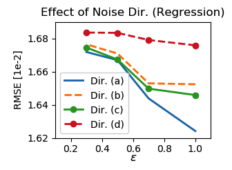
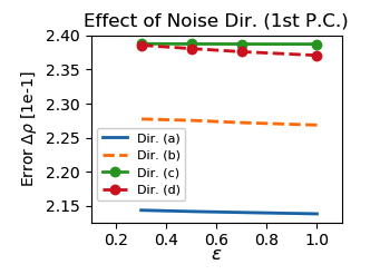
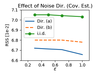
Figure 4: Effect of noise directions on the utility under various $\epsilon$, all with $\delta=1/n$. (Left) Exp. I: regression on the Liver dataset. The four directions shown put more precision budget on the following features based on the domain knowledge [97]: (a) {ALT, Y}, (b) {ALT}, (c) {Y}, (d) {ALT, AST, Y}. (Middle) Exp. II: $1^{st}$ P.C. (with Theorem 2) on the Movement dataset. The four directions emphasize the following features: (a) {ANC0, ANC3}, (b) {ANC0}, (c) {ANC3}, (d) {ANC1, ANC2}. (Right) Exp. III: covariance estimation on the CTG dataset. The two directions emphasize the two disjoint subsets of features: (a) {FHR, ASV, ALV}, (b) The rest of the features.

10 Discussion and Future Works

10.1 Effect of Noise Directions on the Utility

In Section 5.4, we discuss how the choice of noise directions can affect the utility. Here, we investigate this effect on the obtained utility in the three experiments. Figure 4 depicts our results, and we discuss our key observations here.

Figure 4, Left, shows the direction comparison from Exp. I with the directions derived from the domain knowledge [97]. We compare four choices of directions. Direction (a), which uses the domain knowledge (ALT) and the teacher label (Y), yields the best result when compared to: (b) using only the domain knowledge (ALT), (c) using only the teacher label (Y), and (d) using an arbitrary extra feature (ALT+Y+AST). In addition, it is noticeable that the MVG mechanism still generally provides good utility despite the less optimal directions being chosen.

Figure 4, Middle, shows the direction comparison from Exp. II using the MVG mechanism with Theorem 2. We compare four choices of directions. Direction (a), which makes full use of the prior information (ANC0 and ANC3), performs best when compared to: (b), (c) using only partial prior information (ANC0 or ANC3), and (d) having the wrong priors completely (ANC1 and ANC2).

Figure 4, Right, shows the comparison from Exp. III. We compare three choices of directions. Direction (a), which uses the domain knowledge (FHR, ASV, ALV3), gives the best performance compared to: (d) using the completely wrong priors (all other features), and (c) having no prior at all (i.i.d.).

Overall, these observations confirm the merit of both using directional noise for the utility gain, and using prior information to properly select the noise directions. However, we emphasize that, when prior information is not available, we can still exploit the notion of directional noise as shown in Section 9.

10.2 Directional Noise as a Generalized Subspace Analysis

Directional noise provides utility gain by adding less noise in useful directions and more in other directions. This has a connection to subspace projection or dimensionality reduction, in which the non-useful directions are simply removed. Clearly, the main difference between the two is that, in directional noise, the non-useful directions are kept, although are highly perturbed. However, despite being highly perturbed, these directions may still be able to contribute to the utility performance. With dimensionality reduction, which discards them completely, we forfeit that additional information.

We test this hypothesis by running two additional regression experiments (Exp. I) as follows. Given the same two important features used for the MVG mechanism (ALT & Y), we use the Gaussian mechanism [2] and the JL transform method [46] to perform the regression task using only these two features (i.e. discarding the rest of the features). With $\epsilon=1$ and $\delta=\frac{1}{n}$, the results are $(2.538\pm.065)\times 10^{-2}$ and $(2.863\pm.022)\times 10^{-2}$ of RMSE, respectively. Noticeably, these results are significantly worse (i.e. larger error) than that of the MVG mechanism ($(1.624\pm.026)\times 10^{-2}$ or $(1.611\pm.046)\times 10^{-2}$), with the same privacy guarantee. Specifically, by incorporating all features with directional noise via the MVG mechanism, we can achieve over 150% gain in utility over the dimensionality reduction alternatives.

10.3 Information Theoretic Perspective on the MVG Mechanism

In this work, we analyze the MVG mechanism primarily from the perspectives of differential privacy and signal processing. However, as discussed by Cuff and Yu [107], there is a strong connection between differential privacy and information theory. Therefore, in this section, we discuss several advantageous properties of the MVG mechanism from the perspective of information theory. First, we introduce the necessary definitions, concepts, lemmas, and theorems. Second, we discuss how maximizing PNR in Section 7.2 is equivalent to maximizing the mutual information between the MVG mechanism output and the true query answer. Third, we derive the optimal type of query function to be used with the MVG mechanism. Finally, we show that, under a certain condition, not only does the MVG mechanism preserves ($\epsilon,\delta$)-differential privacy, but it also guarantees the minimum correlation between the dataset and the output of the mechanism.

10.3.1 Background Concepts

From the perspective of information theory, we view both the query answer $f(\mathcal{X})$ and the mechanism output $\mathcal{MVG}(f(\mathcal{X}))$ as two random variables. One of the key measurements in information theory concerns the mutual information, defined as follows.

Definition 6 (Mutual information).

Let $\mathcal{X}$ and $\mathcal{Y}$ be two matrix-valued random variables with joint probability density given by $p_{\mathcal{X},\mathcal{Y}}(\mathcal{X},\mathcal{Y})$. Then, the mutual information between $\mathcal{X}$ and $\mathcal{Y}$ is defined as

$$I(\mathcal{X};\mathcal{Y})=\mathbb{E}\left[\log\frac{p_{\mathcal{X},\mathcal{Y}}(\mathcal{X},\mathcal{Y})}{p_{\mathcal{X}}(\mathcal{X})p_{\mathcal{Y}}(\mathcal{Y})}\right].$$

The mutual information $I(\mathcal{X};\mathcal{Y}$) is a non-negative quantity that measures the dependency between the two random variables (cf. [93]). In relation to our analysis, it is important to discuss a property of the mutual information with respect to entropy. To the best of our knowledge, the notion of entropy for a matrix-valued random variable has not been substantially studied. Therefore, we define the terms here, and note that this topic in itself might be of interest for future research in information theory and matrix analysis.

Definition 7.

Given a matrix-valued random variable $\mathcal{X}$ with the pdf $p_{\mathcal{X}}(\mathcal{X})$, the differential entropy is

$$h(\mathcal{X})=\mathbb{E}\left[-\log p_{\mathcal{X}}(\mathcal{X})\right].$$

For a joint pdf $p_{\mathcal{X},\mathcal{Y}}(\mathcal{X},\mathcal{Y})$, the conditional entropy is

$$h(\mathcal{X}\mid\mathcal{Y})=\mathbb{E}\left[-\log p_{\mathcal{X}\mid\mathcal{Y}}(\mathcal{X}\mid\mathcal{Y})\right].$$

For two pdfs $p_{\mathcal{X}}(\mathcal{X})$ and $p_{\mathcal{Y}}(\mathcal{Y})$, the relative entropy is

$$D(p_{\mathcal{X}}\parallel p_{\mathcal{Y}})=\mathbb{E}\left[\log\frac{p_{\mathcal{X}}(\mathcal{X})}{p_{\mathcal{Y}}(\mathcal{Y})}\right].$$

Using the definitions of entropy, the mutual information can be written as

$$I(\mathcal{X};\mathcal{Y})=h(\mathcal{Y})-h(\mathcal{Y}\mid\mathcal{X}).$$ (30)

Next, let us define

$$Cov(vec(\mathcal{X}))=\mathbb{E}\left[[vec(\mathcal{X})-\mathbb{E}\left[vec(\mathcal{X})\right]][vec(\mathcal{X})-\mathbb{E}\left[vec(\mathcal{X})\right]]^{T}\right],$$

and let $\preceq$ be the Loewner partial order defined as follows [62, chapter 7.7].

Definition 8.

Given $\mathbf{A},\mathbf{B}\in\mathbb{R}^{n\times n}$, we write $\mathbf{A}\preceq\mathbf{B}$ if $\mathbf{A}$ and $\mathbf{B}$ are symmetric and $\mathbf{B}-\mathbf{A}$ is positive semi-definite.

Then, we present the following two lemmas.

Lemma 8 (Maximum entropy principle).

Given a matrix-valued random variable $\mathcal{X}\in\mathbb{R}^{m\times n}$ with $Cov(vec(\mathcal{X}))\preceq\mathbf{K}$, the entropy of $\mathcal{X}$ has the property

$$h(\mathcal{X})\leq\frac{1}{2}\log\left[(2\pi e)^{mn}\left|\mathbf{K}\right|\right],$$

with equality if and only if $\mathcal{X}\sim\mathcal{MVG}_{m,n}(\mathbf{M},\boldsymbol{\Sigma},\boldsymbol{\Psi})$ with $\boldsymbol{\Psi}\otimes\boldsymbol{\Sigma}=\mathbf{K}$.

Proof.

The proof parallels the proof in [93], where we use the property that $D(f_{\mathcal{A}}\|g_{\mathcal{X}})$ is non-negative. Let $g_{\mathcal{X}}$ be the pdf of MVG random variable such that $Cov(vec(\mathcal{X}))=Cov(vec(\mathcal{A}))$. We observe that

$$0\leq D(f\|g) =\mathbb{E}\left[\log\frac{f_{\mathcal{A}}(\mathcal{A})}{g_{\mathcal{X}}(\mathcal{A})}\right]=-h(\mathcal{A})-\mathbb{E}\left[\log g_{\mathcal{X}}(\mathcal{A})\right].$$

Next, we show that $\mathbb{E}\left[\log g_{\mathcal{X}}(\mathcal{X})\right]=\mathbb{E}\left[\log g_{\mathcal{X}}(\mathcal{A})\right]$ as follows.

$$\mathbb{E}\left[\log g_{\mathcal{X}}(\mathcal{A})\right] =-\frac{1}{2}\mathbb{E}\left[\mathrm{tr}[\boldsymbol{\Sigma}^{-1}(\mathcal{A}-\mathbf{M})^{T}\boldsymbol{\Psi}^{-1}(\mathcal{A}-\mathbf{M})]\right]+\log\left((2\pi)^{mn/2}\left|\boldsymbol{\Sigma}\right|^{m/2}\left|\boldsymbol{\Psi}\right|^{n/2}\right)$$

$$=-\frac{1}{2}\mathbb{E}\left[(vec(\mathcal{A})-vec(\mathbf{M}))^{T}(\boldsymbol{\Psi}\otimes\boldsymbol{\Sigma})(vec(\mathcal{A})-vec(\mathbf{M}))\right]+\log\left((2\pi)^{mn/2}\left|\boldsymbol{\Psi}\otimes\boldsymbol{\Sigma}\right|\right)$$

$$=-\frac{1}{2}Cov(vec(\mathcal{X}))+\log\left((2\pi)^{\frac{mn}{2}}\left|\boldsymbol{\Psi}\otimes\boldsymbol{\Sigma}\right|\right)=\mathbb{E}\left[\log g_{\mathcal{X}}(\mathcal{X})\right].$$

Using the equality $\mathbb{E}\left[\log g_{\mathcal{X}}(\mathcal{X})\right]=\mathbb{E}\left[\log g_{\mathcal{X}}(\mathcal{A})\right]$, we have $h(\mathcal{A})\leq-\mathbb{E}\left[\log g_{\mathcal{X}}(\mathcal{A})\right]=h(\mathcal{X})$, which concludes the proof. ∎

Lemma 9.

Given two matrix-valued random variables $\mathcal{X}\in\mathbb{R}^{m\times n}$ and $\mathcal{Y}\in\mathbb{R}^{p\times q}$ with $Cov(vec(\mathcal{X})\mid\mathcal{Y})=\mathbf{K}$, the conditional entropy of $\mathcal{X}$ upon $\mathcal{Y}$ has the property

$$h(\mathcal{X}\mid\mathcal{Y})\leq\frac{1}{2}\log\left[(2\pi e)^{mn}\left|\mathbf{K}\right|\right],$$

with equality if and only if $(\mathcal{X},\mathcal{Y})$ is jointly MVG with $Cov(vec(\mathcal{X})\mid\mathcal{Y})=\mathbf{K}$.

Proof.

The proof follows that of Lemma 8 by working with the conditional probability version. ∎

10.3.2 Maximizing PNR is Maximizing Mutual Information

Recall from Section 7.2 that we optimize utility of the MVG mechanism using the PNR criterion. In this section, we present how maximizing PNR is equivalent to maximizing the mutual information between the MVG mechanism output and the true query answer.

Here, we can consider the true query answer $f(\mathcal{X})$, and the mechanism output $\mathcal{MVG}(f(\mathcal{X}))$ as two random variables. Then, we use the mutual information $I(f(\mathcal{X});\mathcal{MVG}(f(\mathcal{X})))$ to measure how informative the MVG mechanism output is, with respect to the true answer. More importantly, we can optimize this measure over the design flexibility of the MVG mechanism as follows:

$$\underset{\mathcal{Z}}{\arg\max}\>I(f(\mathcal{X});f(\mathcal{X})+\mathcal{Z})$$ (31)

$$\text{s.t. }\ \mathcal{Z}\sim\mathcal{MVG}(\mathbf{0},{\bf\boldsymbol{\Sigma}},{\bf\boldsymbol{\Psi}}),\,\mathcal{Z}\in\mathbb{P},$$

where $\mathbb{P}$ is the set of all possible random variables $\mathcal{Z}$ that satisfy ($\epsilon,\delta$)-differential privacy according to Theorem 2, i.e. the conceptual shaded area in Figure 2. If $f(\mathcal{X})$ is Gaussian, the optimization can be simplified as follows.

Lemma 10.

The optimization in Problem 1 is equivalent to

$$\underset{\boldsymbol{\Sigma},\boldsymbol{\Psi}}{\arg\max}\>\frac{|{\bf\boldsymbol{\Psi}}_{f}\otimes\boldsymbol{\Sigma}_{f}+\boldsymbol{\Psi}\otimes\boldsymbol{\Sigma}|}{|\boldsymbol{\Psi}\otimes\boldsymbol{\Sigma}|}$$ (32)

$$\text{s.t. }\ \left\|\boldsymbol{\sigma}(\boldsymbol{\Sigma}^{-1})\right\|_{2}\left\|\boldsymbol{\sigma}(\boldsymbol{\Psi}^{-1})\right\|_{2}\leq \frac{(-\beta+\sqrt{\beta^{2}+8\alpha\epsilon})^{2}}{4\alpha^{2}},$$

where $\left|\cdot\right|$ is the matrix determinant; $\beta$, $\alpha$, and $\epsilon$ are defined in Theorem 2; and $f(\mathcal{X})\sim\mathcal{MVG}(\mathbf{0},{\bf\boldsymbol{\Sigma}}_{f},{\bf\boldsymbol{\Psi}}_{f})$.

Proof.

Because $f(\mathcal{X})$ and $\mathcal{Z}$ are Gaussian, their mutual information can be explicitly evaluated. With the relationship in between the mutual information and entropy in Eq. (30) and Lemma 8, the optimization in Eq. (31) becomes,

$$\underset{\boldsymbol{\Sigma},\boldsymbol{\Psi}}{\arg\max}\frac{1}{2}\log\left(\frac{|{\bf\boldsymbol{\Psi}}_{f}\otimes\boldsymbol{\Sigma}_{f}+\boldsymbol{\Psi}\otimes\boldsymbol{\Sigma}|}{|\boldsymbol{\Psi}\otimes\boldsymbol{\Sigma}|}\right)$$

$$\mathrm{s.t.}\ \left\|\boldsymbol{\sigma}(\boldsymbol{\Sigma}^{-1})\right\|_{2}\left\|\boldsymbol{\sigma}(\boldsymbol{\Psi}^{-1})\right\|_{2}\leq \frac{(-\beta+\sqrt{\beta^{2}+8\epsilon})^{2}}{4\alpha^{2}}.$$

By using the monotonicity property of the log function, this concludes the proof. ∎

Noticeably, comparing Lemma 10 to Problem 1, if we replace $\boldsymbol{\Psi}_{f}\otimes\boldsymbol{\Sigma}_{f}$ with $\mathbf{K}_{f}$, we readily see that the two optimizations are equivalent. In other words, maximizing PNR of the MVG mechanism output is equivalent to maximizing the mutual information between the MVG mechanism output and the true query answer.

10.3.3 Optimal Query Function for the MVG Mechanism

With an alternative view on the formulation of mutual information in Eq. (31), we can also study what type of query function would yield the maximum mutual information between the MVG mechanism output and the true query answer. Here, we prove that such query functions have the form $f(\mathbf{X})=\sum_{i}g_{i}(\mathbf{x}_{i})$, where $\mathbf{x}_{i}$ is the $i^{th}$ column (sample) of $\mathbf{X}$.

Theorem 8.

The mutual information between the true query answer $f(\mathcal{X})$ and the query answer via the MVG mechanism $\mathcal{MVG}(f(\mathcal{X}))$ is maximum when the query function has the form $f(\mathbf{X})=\sum_{i}g_{i}(\mathbf{x}_{i})$, where $\mathbf{x}_{i}$ is the $i^{th}$ column (sample) in $\mathbf{X}$.

Proof.

For clarity, let $\mathcal{Y}=\mathcal{MVG}(f(\mathcal{X}))=f(\mathcal{X})+\mathcal{Z}$. For any query function with $Cov(vec(f(\mathcal{X}))\preceq\mathbf{K}$, write the mutual information in terms of the entropy,

$$\max_{f}I(f(\mathbf{X});\mathcal{Y})=\max_{f}h(\mathcal{Y})-h(\mathcal{Z}).$$

From Lemma 8, the maximum is reached when both $\mathcal{Y}$ and $\mathcal{Z}$ are Gaussian. Since $\mathcal{Z}\sim\mathcal{MVG}_{m,n}(\mathbf{0},\boldsymbol{\Sigma},\boldsymbol{\Psi})$, $\mathcal{Y}$ is Gaussian when $f(\mathbf{X})$ is Gaussian. Then, with the multivariate central limit theorem [108], and a mild condition on $g_{i}(\cdot)$, e.g. $g_{i}(\cdot)$ is bounded, we arrive at the latter condition $f(\mathbf{X})=\sum_{i}g_{i}(\mathbf{x}_{i})$. ∎

Theorem 8 states that to obtain the highest amount of information on the true query answer from the MVG mechanism, the query function should be in the form $f(\mathbf{X})=\sum_{i}g_{i}(\mathbf{x}_{i})$. Conceptually, this condition states that the query function can be decomposed into functions of individual records in the dataset. We note that this can cover a wide range of real-world query functions. Several statistical queries can be formulated in this form including the average, covariance, and correlation. In machine learning, the kernel classifiers and the loss functions can often be formulated in this form [28, 34].

10.3.4 Proof of Minimum Privacy Leakage

Apart from considering the mutual information between the MVG mechanism output and the true query answer as in Eq. (31), we can alternatively consider the mutual information between the MVG mechanism output and the dataset itself. This can be thought of as the correlation between the dataset and the output of the MVG mechanism. From the privacy point of view, clearly, we want this correlation to be minimum. Here, we show that, if the query function has the form $f(\mathbf{X})=\sum g_{i}(\mathbf{x}_{i})$, the MVG mechanism also guarantees the minimum correlation between the dataset and the output of the mechanism.

First, we treat the dataset $\mathcal{X}$ as a random variable. Then, the claim is readily proved by the following theorem.

Theorem 9.

If the matrix-valued query function is of the form $f(\mathbf{X})=\sum g_{i}(\mathbf{x}_{i})$, then for an arbitrary positive definite matrix $\mathbf{K}$,

$$\min_{\mathcal{Z}:Cov(vec(\mathcal{Z}))=\mathbf{K}}I(\mathcal{X};f(\mathcal{X})+\mathcal{Z})=I(\mathcal{X};f(\mathcal{X})+\mathcal{Z}_{\mathcal{MVG}}),$$

where $\mathcal{Z}_{\mathcal{MVG}}\sim\mathcal{MVG}_{m,n}(\mathbf{0},\boldsymbol{\Sigma},\boldsymbol{\Psi})$ such that $\boldsymbol{\Psi}\otimes\boldsymbol{\Sigma}=\mathbf{K}$.

Proof.

First, we use the multivariate central limit theorem [108] to claim that $f(\mathcal{X})$ is Gaussian. Then, using the decomposition in Eq. (30), we have that

$$I(\mathcal{X};f(\mathcal{X})+\mathcal{Z}) =h(f(\mathcal{X})+\mathcal{Z})-h(f(\mathcal{X})+\mathcal{Z}|\mathcal{X})$$

$$=h(f(\mathcal{X})+\mathcal{Z})-h(f(\mathcal{X})+\mathcal{Z}|f(\mathcal{X}))$$

$$=I(f(\mathcal{X});f(\mathcal{X})+\mathcal{Z})$$

$$=h\left(f(\mathcal{X})\right)-h\left(f(\mathcal{X})|f(\mathcal{X})+\mathcal{Z}\right),$$

where the second line follows from the independence of $f(\mathcal{X})$ and $\mathcal{Z}$, and from the fact that by conditioning on $\mathcal{X}$, we have $h(f(\mathcal{X})+\mathcal{Z}\mid\mathcal{X})=h(\mathcal{Z})$. Therefore, we have

$$\min_{\mathcal{Z}:Cov(vec(\mathcal{Z}))=\mathbf{K}}I(\mathcal{X};f(\mathcal{X})+\mathcal{Z}) =h\left(f(\mathcal{X})\right)-\max_{\mathcal{Z}:Cov(vec(\mathcal{Z}))=\mathbf{K}}h\left(f(\mathcal{X})|f(\mathcal{X})+\mathcal{Z}\right)$$

$$=h\left(f(\mathcal{X})\right)-h\left(f(\mathcal{X})|f(\mathcal{X})+\mathcal{Z}_{\mathcal{MVG}}\right),$$

where the last step follows from Lemma 9. ∎

Combining result of Theorem 2 and Theorem 9, we have a remarkable observation that not only does the MVG mechanism guarantees $(\epsilon,\delta)$-differential privacy but it also guarantees the minimum possible correlation (in terms of mutual information) between the database and the output of the mechanism. Finally, we note that the result of Theorem (9) is very general as it does not assume anything about the distribution of the dataset $\mathcal{X}$ at all.

11 Conclusion

In this work, we study the matrix-valued query function in differential privacy. We present the MVG mechanism that can fully exploit the structural nature of the matrix-valued analysis. We present two sufficient conditions for the MVG mechanism to guarantee $(\epsilon,\delta)$-differential privacy – one for the general matrix-valued query function, and another for the positive semi-definite query function. As a result of the sufficient conditions, we introduce the novel concept of directional noise, which can be used to reduce the impact of the noise on the utility of the query answer. Furthermore, we show how design the directional noise such that the power-to-noise ratio (PNR) of the MVG mechanism output is maximum. Finally, we evaluate our approach experimentally for three matrix-valued query functions on three privacy-sensitive datasets. The results show that our approach can provide significant utility improvement over existing methods, and yield the utility performance close to that of the non-private baseline while preserving $(1.0,1/n)$-differential privacy. We hope that our work may inspire further development in the problem of differential privacy under matrix-valued query functions.

References

- [1] T. Chanyaswad, A. Dytso, H. V. Poor, and P. Mittal, “Mvg mechanism: Differential privacy under matrix-valued query,” arXiv preprint arXiv:1801.00823, 2018.
- [2] C. Dwork, K. Kenthapadi, F. McSherry, I. Mironov, and M. Naor, “Our data, ourselves: Privacy via distributed noise generation,” in EUROCRYPT. Springer, 2006.
- [3] C. Dwork, F. McSherry, K. Nissim, and A. Smith, “Calibrating noise to sensitivity in private data analysis,” in TCC. Springer, 2006.
- [4] C. Dwork, Differential privacy, ser. Automata, languages and programming. Springer, 2006, pp. 1–12.
- [5] F. McSherry and K. Talwar, “Mechanism design via differential privacy,” in FOCS. IEEE, 2007.
- [6] X. Xiao, G. Wang, and J. Gehrke, “Differential privacy via wavelet transforms,” IEEE TKDE, vol. 23, no. 8, pp. 1200–1214, 2011.
- [7] M. Hay, V. Rastogi, G. Miklau, and D. Suciu, “Boosting the accuracy of differentially private histograms through consistency,” PVLDB, vol. 3, no. 1-2, pp. 1021–1032, 2010.
- [8] W. Qardaji, W. Yang, and N. Li, “Understanding hierarchical methods for differentially private histograms,” PVLDB, vol. 6, no. 14, pp. 1954–1965, 2013.
- [9] C. Li, M. Hay, G. Miklau, and Y. Wang, “A data-and workload-aware algorithm for range queries under differential privacy,” PVLDB, vol. 7, no. 5, pp. 341–352, 2014.
- [10] X. Zhang, R. Chen, J. Xu, X. Meng, and Y. Xie, “Towards accurate histogram publication under differential privacy,” in SDM. SIAM, 2014.
- [11] Y. Xiao, L. Xiong, L. Fan, and S. Goryczka, “Dpcube: differentially private histogram release through multidimensional partitioning,” arXiv:1202.5358, 2012.
- [12] G. Cormode, C. Procopiuc, D. Srivastava, E. Shen, and T. Yu, “Differentially private spatial decompositions,” in ICDE. IEEE, 2012.
- [13] W. Qardaji, W. Yang, and N. Li, “Differentially private grids for geospatial data,” in ICDE. IEEE, 2013.
- [14] J. Xu, Z. Zhang, X. Xiao, Y. Yang, G. Yu, and M. Winslett, “Differentially private histogram publication,” The VLDB Journal, vol. 22, no. 6, pp. 797–822, 2013.
- [15] G. Acs, C. Castelluccia, and R. Chen, “Differentially private histogram publishing through lossy compression,” in ICDM. IEEE, 2012.
- [16] K. Nissim, S. Raskhodnikova, and A. Smith, “Smooth sensitivity and sampling in private data analysis,” in STOC. ACM, 2007.
- [17] M. Hardt and G. N. Rothblum, “A multiplicative weights mechanism for privacy-preserving data analysis,” in FOCS. IEEE, 2010.
- [18] M. Hardt, K. Ligett, and F. McSherry, “A simple and practical algorithm for differentially private data release,” in NIPS, 2012.
- [19] C. Li, M. Hay, V. Rastogi, G. Miklau, and A. McGregor, “Optimizing linear counting queries under differential privacy,” in PODS. ACM, 2010.
- [20] C. Li and G. Miklau, “An adaptive mechanism for accurate query answering under differential privacy,” PVLDB, vol. 5, no. 6, pp. 514–525, 2012.
- [21] G. Yuan, Z. Zhang, M. Winslett, X. Xiao, Y. Yang, and Z. Hao, “Low-rank mechanism: optimizing batch queries under differential privacy,” PVLDB, vol. 5, no. 11, pp. 1352–1363, 2012.
- [22] M. Lyu, D. Su, and N. Li, “Understanding the sparse vector technique for differential privacy,” arXiv:1603.01699, 2016.
- [23] C. Dwork, G. N. Rothblum, and S. Vadhan, “Boosting and differential privacy,” in FOCS. IEEE, 2010.
- [24] C. Dwork, “Differential privacy: A survey of results,” in TAMC. Springer, 2008.
- [25] C. Dwork, K. Talwar, A. Thakurta, and L. Zhang, “Analyze gauss: optimal bounds for privacy-preserving principal component analysis,” in STOC. ACM, 2014.
- [26] A. Blum, C. Dwork, F. McSherry, and K. Nissim, “Practical privacy: the sulq framework,” in PODS. ACM, 2005.
- [27] K. Chaudhuri, A. Sarwate, and K. Sinha, “Near-optimal differentially private principal components,” in NIPS, 2012.
- [28] S. Y. Kung, Kernel Methods and Machine Learning. Cambridge University Press, 2014.
- [29] C. Godsil and G. F. Royle, Algebraic graph theory. Springer Science & Business Media, 2013, vol. 207.
- [30] J. F. Hughes, A. V. Dam, J. D. Foley, and S. K. Feiner, Computer graphics: principles and practice. Pearson Education, 2014.
- [31] W. C. Thacker, “The role of the hessian matrix in fitting models to measurements,” JGR: Oceans, vol. 94, no. C5, pp. 6177–6196, 1989.
- [32] W. R. Gilks, S. Richardson, and D. Spiegelhalter, Markov chain Monte Carlo in practice. CRC press, 1995.
- [33] S. R. White, “Density matrix formulation for quantum renormalization groups,” PRL, vol. 69, no. 19, p. 2863, 1992.
- [34] J. Friedman, T. Hastie, and R. Tibshirani, The elements of statistical learning. Springer series in statistics New York, 2001, vol. 1.
- [35] V. Vapnik, The nature of statistical learning theory. Springer science & business media, 2013.
- [36] Wikipedia, “Matrix (mathematics),” https://en.wikipedia.org/wiki/Matrix_(mathematics), 17 April 2017 2017.
- [37] C. Dwork and A. Roth, “The algorithmic foundations of differential privacy,” FnT-TCS, vol. 9, no. 3-4, pp. 211–407, 2014.
- [38] M. Lichman, “Uci machine learning repository,” http://archive.ics.uci.edu/ml, 2013.
- [39] R. Forsyth and R. Rada, Machine learning: applications in expert systems and information retrieval. Halsted Press, 1986.
- [40] D. Bacciu, P. Barsocchi, S. Chessa, C. Gallicchio, and A. Micheli, “An experimental characterization of reservoir computing in ambient assisted living applications,” Neural Computing and Applications, vol. 24, no. 6, pp. 1451–1464, 2014.
- [41] D. A. de Campos, J. Bernardes, A. Garrido, J. M. de Sa, and L. Pereira-Leite, “Sisporto 2.0: a program for automated analysis of cardiotocograms,” Journal of Maternal-Fetal Medicine, vol. 9, no. 5, pp. 311–318, 2000.
- [42] J. Blocki, A. Blum, A. Datta, and O. Sheffet, “The johnson-lindenstrauss transform itself preserves differential privacy,” in FOCS. IEEE, 2012.
- [43] F. Liu, “Generalized gaussian mechanism for differential privacy,” arXiv:1602.06028, 2016.
- [44] A. Blum and A. Roth, Fast private data release algorithms for sparse queries, ser. Approximation, Randomization, and Combinatorial Optimization. Algorithms and Techniques. Springer, 2013, pp. 395–410.
- [45] J. Upadhyay, “Randomness efficient fast-johnson-lindenstrauss transform with applications in differential privacy and compressed sensing,” arXiv:1410.2470, 2014.
- [46] ——, “Circulant matrices and differential privacy,” analysis, vol. 16, p. 47, 2014.
- [47] N. Johnson, J. P. Near, and D. Song, “Practical differential privacy for sql queries using elastic sensitivity,” arXiv:1706.09479, 2017.
- [48] M. Hay, A. Machanavajjhala, G. Miklau, Y. Chen, and D. Zhang, “Principled evaluation of differentially private algorithms using dpbench,” in SIGMOD/PODS. ACM, 2016.
- [49] D. Proserpio, S. Goldberg, and F. McSherry, “Calibrating data to sensitivity in private data analysis: a platform for differentially-private analysis of weighted datasets,” PVLDB, vol. 7, no. 8, pp. 637–648, 2014.
- [50] W.-Y. Day and N. Li, “Differentially private publishing of high-dimensional data using sensitivity control,” in CCS. ACM, 2015.
- [51] K. Kenthapadi, A. Korolova, I. Mironov, and N. Mishra, “Privacy via the johnson-lindenstrauss transform,” arXiv:1204.2606, 2012.
- [52] T. Chanyaswad, C. Liu, and P. Mittal, “Coupling dimensionality reduction with generative model for non-interactive private data release,” arXiv:1709.00054, 2017.
- [53] C. Xu, J. Ren, Y. Zhang, Z. Qin, and K. Ren, “Dppro: Differentially private high-dimensional data release via random projection,” IEEE TIFS, 2017.
- [54] Y. D. Li, Z. Zhang, M. Winslett, and Y. Yang, “Compressive mechanism: Utilizing sparse representation in differential privacy,” in WPES. ACM, 2011.
- [55] X. Jiang, Z. Ji, S. Wang, N. Mohammed, S. Cheng, and L. Ohno-Machado, “Differential-private data publishing through component analysis,” Trans. on Data Privacy, vol. 6, no. 1, pp. 19–34, Apr 2013.
- [56] A. P. Dawid, “Some matrix-variate distribution theory: notational considerations and a bayesian application,” Biometrika, vol. 68, no. 1, pp. 265–274, 1981.
- [57] A. Gupta and T. Varga, “Characterization of matrix variate normal distributions,” Journal of Multivariate Analysis, vol. 41, no. 1, pp. 80–88, 1992.
- [58] T. T. Nguyen, “A note on matrix variate normal distribution,” Journal of Multivariate Analysis, vol. 60, no. 1, pp. 148–153, 1997.
- [59] P. Dutilleul, “The mle algorithm for the matrix normal distribution,” Journal of statistical computation and simulation, vol. 64, no. 2, pp. 105–123, 1999.
- [60] A. Iranmanesh, M. Arashi, and S. Tabatabaey, “On conditional applications of matrix variate normal distribution,” Iranian Journal of Mathematical Sciences and Informatics, vol. 5, no. 2, pp. 33–43, 2010.
- [61] D. D. Waal, “Matrix-valued distributions,” Encyclopedia of statistical sciences, 2006.
- [62] R. A. Horn and C. R. Johnson, Matrix analysis. Cambridge university press, 2012.
- [63] B. Laurent and P. Massart, “Adaptive estimation of a quadratic functional by model selection,” Annals of Statistics, pp. 1302–1338, 2000.
- [64] J. K. Merikoski, H. Sarria, and P. Tarazaga, “Bounds for singular values using traces,” Linear Algebra and its Applications, vol. 210, pp. 227–254, 1994.
- [65] J. von Neumann, “Some matrix inequalities and metrization of metric space,” Tomsk Univ.Rev, vol. 1, pp. 286–296, 1937.
- [66] R. A. Horn and C. R. Johnson, “Topics in matrix analysis, 1991,” Cambridge University Press, vol. 37, p. 39, 1991.
- [67] J. Hadamard, “Étude sur les propriétés des fonctions entières et en particulier d’une fonction considérée par riemann,” Journal de mathématiques pures et appliquées, pp. 171–216, 1893.
- [68] C. D. Meyer, Matrix analysis and applied linear algebra. Siam, 2000, vol. 2.
- [69] F. Liu, “Model-based differential private data synthesis,” arXiv:1606.08052, 2016.
- [70] S. Zhou, K. Ligett, and L. Wasserman, “Differential privacy with compression,” in ISIT. IEEE, 2009.
- [71] J. Sondow and E. W. Weisstein, “Harmonic number,” http://mathworld.wolfram.com/HarmonicNumber.html, March 23, 2017 2017.
- [72] B. Scholkopf and A. J. Smola, Learning with kernels: support vector machines, regularization, optimization, and beyond. MIT press, 2001.
- [73] D. E. Muller, “A method for solving algebraic equations using an automatic computer,” Mathematical tables and other aids to computation, vol. 10, no. 56, pp. 208–215, 1956.
- [74] F. Viète, “Opera mathematica,” Lvgdvni Batavorvm, ex off. B. and A. Elzeviriorum, 1646.
- [75] A. Girard, Invention nouvelle en l’algebre. Blauew, 1629, vol. 1.
- [76] A. Meenakshi and C. Rajian, “On a product of positive semidefinite matrices,” Linear algebra and its applications, vol. 295, no. 1-3, pp. 3–6, 1999.
- [77] K. P. Murphy, Machine Learning: A Probabilistic Perspective. The MIT Press, 2012.
- [78] C. M. Bishop, “Pattern recognition,” Machine Learning, vol. 128, 2006.
- [79] H. Abdi, “Singular value decomposition (svd) and generalized singular value decomposition,” Encyclopedia of Measurement and Statistics. Thousand Oaks (CA): Sage, pp. 907–912, 2007.
- [80] M. Fredrikson, E. Lantz, S. Jha, S. Lin, D. Page, and T. Ristenpart, “Privacy in pharmacogenetics: An end-to-end case study of personalized warfarin dosing.” in USENIX Security, 2014.
- [81] M. Hardt and A. Roth, “Beyond worst-case analysis in private singular vector computation,” in STOC. ACM, 2013.
- [82] M. Kapralov and K. Talwar, “On differentially private low rank approximation,” in SODA. SIAM, 2013.
- [83] Netflix, “Netflix prize,” http://www.netflixprize.com/.
- [84] A. Narayanan and V. Shmatikov, “Robust de-anonymization of large sparse datasets,” in S&P. IEEE, 2008.
- [85] R. M. Bell, Y. Koren, and C. Volinsky, “The bellkor 2008 solution to the netflix prize,” Statistics Research Department at AT&T Research, 2008.
- [86] F. McSherry and I. Mironov, “Differentially private recommender systems: building privacy into the net,” in KDD. ACM, 2009.
- [87] A. Genz, F. Bretz, T. Miwa, X. Mi, F. Leisch, F. Scheip, B. Bornkamp, M. Maechler, and T. Hothorn, “Package mvtnorm,” http://mvtnorm.R-forge.R-project.org, 02/02/2016 2016.
- [88] SciPy.org, “scipy.stats.multivariate_normal,” https://docs.scipy.org/doc/scipy-0.14.0/reference/generated/scipy.stats.multivariate\_normal.html, 5/11/2014 2014.
- [89] J. Burkardt, “Normal_dataset: Generate multivariate normal random datasets,” https://people.sc.fsu.edu/~jburkardt/cpp_src/normal_dataset/normal_dataset.html, 12/9/2009 2009.
- [90] G. H. Golub and C. F. V. Loan, “Matrix computations,” Johns Hopkins University, Press, Baltimore, MD, USA, pp. 374–426, 1996.
- [91] D. H. Johnson, “Signal-to-noise ratio,” Scholarpedia, vol. 1, no. 12, p. 2088, 2006.
- [92] L. Tan and J. Jiang, Digital signal processing: fundamentals and applications. Academic Press, 2013.
- [93] T. M. Cover and J. A. Thomas, Elements of information theory. John Wiley & Sons, 2012.
- [94] K. Schacke, “On the kronecker product,” Master’s thesis, University of Waterloo, 2004.
- [95] O. Rojo, R. Soto, and H. Rojo, “Bounds for the spectral radius and the largest singular value,” Computers & Mathematics with Applications, vol. 36, no. 1, pp. 41–50, 1998.
- [96] D. Chafai, “Singular values of random matrices,” Lecture Notes, 2009.
- [97] P. I. Alatalo, H. M. Koivisto, J. P. Hietala, K. S. Puukka, R. Bloigu, and O. J. Niemela, “Effect of moderate alcohol consumption on liver enzymes increases with increasing body mass index,” AJCN, vol. 88, no. 4, pp. 1097–1103, Oct 2008.
- [98] C. C. Santos, J. Bernardes, P. M. Vitányi, and L. Antunes, “Clustering fetal heart rate tracings by compression,” in CBMS. IEEE, 2006.
- [99] J. McDermott and R. S. Forsyth, “Diagnosing a disorder in a classification benchmark,” Pattern Recognition Letters, vol. 73, pp. 41–43, 2016.
- [100] F. Pedregosa, G. Varoquaux, A. Gramfort, V. Michel, B. Thirion, O. Grisel, M. Blondel, P. Prettenhofer, R. Weiss, and V. Dubourg, “Scikit-learn: Machine learning in python,” JMLR, vol. 12, no. Oct, pp. 2825–2830, 2011.
- [101] K. Chaudhuri and S. A. Vinterbo, “A stability-based validation procedure for differentially private machine learning,” in NIPS, 2013.
- [102] I. T. Jolliffe, Principal Component Analysis and Factor Analysis, ser. Principal component analysis. Springer, 1986, pp. 115–128.
- [103] C. R. Rao, “The use and interpretation of principal component analysis in applied research,” Sankhya: The Indian Journal of Statistics, Series A, pp. 329–358, 1964.
- [104] A. Blum, K. Ligett, and A. Roth, “A learning theory approach to noninteractive database privacy,” JACM, vol. 60, no. 2, p. 12, 2013.
- [105] J. C. Duchi, M. I. Jordan, and M. J. Wainwright, “Local privacy and statistical minimax rates,” in FOCS. IEEE, 2013.
- [106] S. E. Fienberg, A. Rinaldo, and X. Yang, “Differential privacy and the risk-utility tradeoff for multi-dimensional contingency tables,” in PSD. Springer, 2010.
- [107] P. Cuff and L. Yu, “Differential privacy as a mutual information constraint,” in CCS. ACM, 2016.
- [108] M. G. Hahn and M. J. Klass, “The multidimensional central limit theorem for arrays normed by affine transformations,” The Annals of Probability, pp. 611–623, 1981.