sectioning ection]subsection captionlabel

The decreasing enumeration of the points of a Poisson random measure whose mean measure is Radon on $(0,\infty]$ can be represented as a non-increasing function of the jump times of a standard Poisson process. This observation allows to generalize the essential idea from a well-known exact simulation algorithm for arbitrary extreme-value copulas to copulas of a more general family of max-infinitely divisible distributions, with reciprocal Archimedean copulas being a particular example.

1 Introduction

A copula $C:[0,1]^{d}\rightarrow[0,1]$ is a multivariate distribution function of a random vector whose components are all uniformly distributed on $[0,1]$, cf. [Nelsen (2006)] for background. The family of reciprocal Archimedean copulas has been introduced and analyzed in [Genest et al. (2018)]. With a parameterizing univariate distribution function $F:[0,\infty)\rightarrow[0,1]$, a copula in this class has the analytical form

$$C_{F}(u_{1},\ldots,u_{d})=\prod_{A\in\mathcal{P}_{d,o}}F\Big{(}\sum_{k\in A}F^{-1}(u_{k})\Big{)}\Big{/}\prod_{A\in\mathcal{P}_{d,e}}F\Big{(}\sum_{k\in A}F^{-1}(u_{k})\Big{)},$$

where $\mathcal{P}_{d,o}$ (resp. $\mathcal{P}_{d,e}$) is the set of all non-empty subsets of $\{1,\ldots,d\}$ with odd (resp. even) cardinality. The nomenclature of this copula family is justified by some striking analogies with the well-understood family of Archimedean copulas, cf. [McNeil, Nešlehová (2009)] for background on the latter. For instance, [Genest et al. (2018)] show that $C_{F}$ is a proper copula in dimension $d$ if and only if the parameterizing function $F:[0,\infty)\rightarrow[0,\infty)$ has the form

$$F(t)=\exp\Big{(}-\int_{t}^{\infty}\big{(}1-\frac{t}{x}\big{)}^{d-1}\,\nu(\mathrm{d}x)\Big{)}=:\exp\big{(}-\Lambda(t)\big{)},$$

with $\nu$ a non-finite Radon measure on $(0,\infty]$ such that $\nu(\{\infty\})=0$, called the radial measure. In this case, a random vector $\mathbf{Y}=(Y_{1},\ldots,Y_{d})$ with distribution function $C_{F}\big{(}F(t_{1}),\ldots,F(t_{d})\big{)}$ has stochastic representation

$$\mathbf{Y}=\Bigg{(}\max_{k\geq 1}\Big{\{}R_{k}\,Q_{1}^{(k)}\Big{\}},\ldots,\max_{k\geq 1}\Big{\{}R_{k}\,Q_{d}^{(k)}\Big{\}}\Bigg{)},$$ (1)

where $\mathbf{Q}^{(k)}=(Q_{1}^{(k)},\ldots,Q_{d}^{(k)})$, $k\in\mathbb{N}$, are independent and uniformly distributed on the $d$-dimensional simplex $S_{d}:=\{\mathbf{q}=(q_{1},\ldots,q_{d})\geq 0\,:\,q_{1}+\ldots+q_{d}=1\}$, and, independently, $\{R_{k}\}_{k\geq 1}$ is an enumeration of the points of a Poisson random measure on $(0,\infty]$ with mean measure $\nu$. It is important to notice that the index $k$ in this maximum runs through an enumeration of the points $\{R_{k}\}_{k\geq 1}$ of the Poisson random measure. This collection of points is almost surely countably infinite since the measure $\nu$ is non-finite. The most prominent member of the family of reciprocal Archimedean copulas is the Galambos copula, the terminology dating back to [Galambos (1975)], which arises for the choice $\nu(\mathrm{d}x)=\Gamma(d+1/\theta)/(\Gamma(d)\,\Gamma(1/\theta))\,x^{-1/\theta-1}\,\mathrm{d}x$, cf. [Genest et al. (2018), Example 5]. Further background on the Galambos copula can be found in [Mai (2014)].

The stochastic representation (1) is difficult to simulate from due to the infinite maximum, which is why [Genest et al. (2018)] only propose an approximative simulation strategy. For extreme-value copulas, a family whose intersection with reciprocal Archimedean copulas equals the Galambos copula, an alternative and exact simulation strategy is developed in [Dombry et al. (2016)], based on an idea originally due to [Schlather (2002)]. Section 2 shows how the idea of this algorithm can be generalized to include arbitrary reciprocal Archimedean copulas. Section 3 concludes.

2 Exact simulation of reciprocal Archimedean copulas

Let $\nu$ be a Radon measure on $(0,\infty]$, i.e. $S(t):=\nu((t,\infty])<\infty$ for all $t>0$, with the property that $\nu(\{\infty\})=0$. We denote $u_{\nu}:=\nu\big{(}(0,\infty]\big{)}$ and define a pseudo-inverse via

$$S^{-1}(t):=\inf\{x>0\,:\,S(x)\leq t\},\quad t\in[0,u_{\nu}].$$

For later reference we remark that right-continuity of $S$ implies

$$y<S(x)\,\Leftrightarrow\,S^{-1}(y)>x,\quad x\in(0,\infty),\,y\in[0,u_{\nu}].$$ (2)

We explicitly allow $\nu$ to be finite here, in which case $S^{-1}(t)$ is only defined for $t\leq u_{\nu}<\infty$, but for the application to reciprocal Archimedean copulas only the case when $u_{\nu}=\infty$ is relevant. For $x>0$ we denote by $\delta_{x}$ the Dirac measure at $x$. We denote by $P=\sum_{k=1}^{N}\delta_{R_{k}}$ a Poisson random measure on $(0,\infty]$ with mean measure $\nu$, the random variable $N\in\mathbb{N}_{0}\cup\{\infty\}$ representing the number of points $\{R_{k}\}$ of $P$. [Resnick (1987)] is an excellent textbook for background on Poisson random measures. The most important, and characterizing, property of a Poisson random measure on a measurable space $E$ with mean measure $\nu$ is the Laplace functional formula

$$\mathbb{E}\Big{[}e^{-\int_{E}f(x)\,P(\mathrm{d}x)}\Big{]}=\exp\Big{(}-\int_{E}\big{(}1-e^{-f(x)}\big{)}\,\nu(\mathrm{d}x)\Big{)},$$ (3)

where $\nu$ is a Radon measure on $E$, and $f$ is a non-negative, Borel-measurable function on $E$. Recall that if $\nu$ is non-finite, $P$ has countably many points $R_{1},R_{2},\ldots$. But if $\nu$ is finite, the number of points $N$ has a Poisson distribution with parameter $u_{\nu}$. Hence, regarding notation it is convenient for us to treat both cases jointly by denoting the points of $P$ by $R_{1},\ldots,R_{N}$, possibly allowing for the value $N=\infty$ in case of non-finite $\nu$. Without loss of generality, we further enumerate the points $R_{k}$ such that $R_{1}\geq R_{2}\geq\ldots$ almost surely.

The following auxiliary result follows from (3) by a change of variables from (the possibly complicated measure) $\nu(\mathrm{d}x)$ to the Lebesgue measure $\mathrm{d}x$, resulting in a stochastic representation of $\{R_{k}\}$ that is convenient for our purpose of simulating reciprocal Archimedean copulas. Even though this computation is presumably standard in the literature on Poisson random measures, we state it as a separate lemma and provide a proof here, because it is educational, one key ingredient for the derived simulation algorithm, and apparently lesser known in the literature on copulas and dependence modeling.

Lemma 2.1 (Stochastic representation of $\{R_{k}\}$)

Let $\{\epsilon_{k}\}_{k\in\mathbb{N}}$ be a sequence of independent and identically distributed exponential random variables with unit mean. Introducing the random variable

$$N_{\epsilon}:=\begin{cases}\infty&\mbox{if }u_{\nu}=\infty,\\ \sum_{k\geq 1}1_{\{\epsilon_{1}+\ldots+\epsilon_{k}\leq u_{\nu}\}}&\mbox{else,}\\ \end{cases},$$

we have the distributional equality

$$\{R_{k}\}_{k=1,\ldots,N}\stackrel{{\scriptstyle d}}{{=}}\{S^{-1}(\epsilon_{1}+\ldots+\epsilon_{k})\}_{k=1,\ldots,N_{\epsilon}}.$$

Proof

Define the point measure $\hat{P}:=\sum_{k=1}^{N_{\epsilon}}\delta_{S^{-1}(\epsilon_{1}+\ldots+\epsilon_{k})}$. We notice that $\tilde{P}=\sum_{k\geq 1}\delta_{\epsilon_{1}+\ldots+\epsilon_{k}}$ equals a Poisson random measure on $[0,\infty)$ with mean measure the Lebesgue measure $\mathrm{d}x$, hence

$$\mathbb{E}\Big{[}e^{-\int_{(0,\infty]}f(x)\,\hat{P}(\mathrm{d}x)}\Big{]}=\mathbb{E}\Big{[}e^{-\sum_{k=1}^{N_{\epsilon}}f\big{(}S^{-1}(\epsilon_{1}+\ldots+\epsilon_{k})\big{)}}\Big{]}$$

$$\quad=\mathbb{E}\Big{[}e^{-\int_{[0,\infty)}f\big{(}S^{-1}(x)\big{)}\,1_{\{x\leq u_{\nu}\}}\,\tilde{P}(\mathrm{d}x)}\Big{]}$$

$$\quad\stackrel{{\scriptstyle(\ref{laplace})}}{{=}}\exp\Big{(}-\int_{[0,\infty)}\big{(}1-e^{-f\big{(}S^{-1}(x)\big{)}\,1_{\{x\leq u_{\nu}\}}}\big{)}\,\mathrm{d}x\Big{)}$$

$$\quad=\exp\Big{(}-\int_{0}^{u_{\nu}}\big{(}1-e^{-f\big{(}S^{-1}(x)\big{)}}\big{)}\,\mathrm{d}x\Big{)}\stackrel{{\scriptstyle(\ast)}}{{=}}\exp\Big{(}-\int_{0}^{\infty}\big{(}1-e^{-f(x)}\big{)}\,\nu(\mathrm{d}x)\Big{)}$$

$$\quad\stackrel{{\scriptstyle(\ref{laplace})}}{{=}}\mathbb{E}\Big{[}e^{-\int_{(0,\infty]}f(x)\,{P}(\mathrm{d}x)}\Big{]}.$$

To verify equation $(\ast)$, denote by $\lambda$ the Lebesgue measure on $(0,\infty)$, and observe that the map $G:=S^{-1}:\big{(}0,u_{\nu})\rightarrow(0,\infty)$ is measurable. Consider the measure $G_{\lambda}$ defined by $G_{\lambda}(E):=\lambda(G^{-1}(E))$, $E$ a Borel set in $(0,\infty)$ and $G^{-1}(E)$ its pre-image under $G$ in $(0,u_{\nu})$. Then we observe for $x\in(0,\infty)$ that

$$G_{\lambda}\big{(}(x,\infty]\big{)} =\lambda\big{(}\{y\in(0,u_{\nu})\,:\,S^{-1}(y)>x\}\big{)}\stackrel{{\scriptstyle(\ref{geninv})}}{{=}}\lambda\big{(}\{y\in(0,u_{\nu})\,:\,y<S(x)\}\big{)}$$

$$=S(x)=\nu((x,\infty]).$$

Consequently, $G_{\lambda}=\nu$ and we have the measure-theoretic change of variable formula

$$\int_{(0,\infty)}g(x)\,\nu(\mathrm{d}x) =\int_{(0,\infty)}g(x)\,G_{\lambda}(\mathrm{d}x)=\int_{(0,u_{\nu})}g\big{(}G(x)\big{)}\,\lambda(\mathrm{d}x)$$

$$=\int_{0}^{u_{\nu}}g\big{(}S^{-1}(x)\big{)}\,\mathrm{d}x.$$

Applying it to the function $g(x)=1-e^{-f(x)}$ implies $(\ast)$. The claim now follows from uniqueness of the Laplace functional of Poisson random measure, since $f$ was an arbitrary non-negative, Borel-measurable function. $\Box$

Remark 2.2 (Simulation of infinitely divisible laws on $[0,\infty)$)

It is not the first time that the change of variables technique of Lemma 2.1 is found useful for an application to simulation. To provide another example, [Bondesson (1982)] uses essentially the same technique to represent a non-negative infinitely divisible random variable $X$ with associated Lévy measure $\nu$ as

$$X=\sum_{k=1}^{N}R_{k}\stackrel{{\scriptstyle d}}{{=}}\sum_{k=1}^{N_{\epsilon}}S^{-1}(\epsilon_{1}+\ldots+\epsilon_{k})$$

and discusses the possibility to simulate $X$ based on this stochastic representation.

If the radial measure $\nu$ is absolutely continuous with positive density on $(0,\infty)$, the function $S$ is continuous and strictly decreasing and $S^{-1}$ is the regular inverse. The following example sheds some light on the situation in the case of discrete measures $\nu$.

Example 2.3 (Discrete radial measures)

Let $\infty>a_{1}>a_{2}>\ldots>0$ with $\lim_{k\rightarrow\infty}a_{k}=0$ and $b_{k}\geq 0$ with $\sum_{k\geq 1}b_{k}=\infty$ (to guarantee that $\nu$ is non-finite), and consider $\nu=\sum_{k\geq 1}b_{k}\,\delta_{a_{k}}$ on $(0,\infty)$, obviously Radon on $(0,\infty]$. The functions $S$ and $S^{-1}$ in this case are given by

$$S(t) =\sum_{k\geq 1}\Big{(}\sum_{i=1}^{k}b_{i}\Big{)}\,1_{[a_{k+1},a_{k})}(t),\quad t\geq 0,$$

$$S^{-1}(t) =\sum_{k\geq 1}a_{k}\,1_{\big{[}\sum_{i=1}^{k-1}b_{i},\sum_{i=1}^{k}b_{i}\big{)}}(t),\quad t\geq 0.$$

As a concrete one-parametric example, let $\theta>0$ and $a_{k}=1/k$, $b_{k}=\theta$, $k\geq 1$. It is not difficult to observe that in this case the formulas above boil down to

$$S(t)=\lim_{u\downarrow t}\theta\,\Big{\lfloor}\frac{1}{u}\Big{\rfloor},\quad S^{-1}(t)=1/{\Big{\lceil}\frac{t}{\theta}\Big{\rceil}},$$

with $\lfloor.\rfloor$ and $\lceil.\rceil$ denoting the usual floor and ceiling functions mapping $[0,\infty)$ to $\mathbb{N}_{0}$. The associated distribution function $F=\exp(-\Lambda)$ generating the $d$-dimensional reciprocal Archimedean copula associated with $\nu$ is determined by

$$\Lambda(t)=\theta\,\sum_{k=1}^{\lfloor 1/t\rfloor}\big{(}1-k\,t\big{)}^{d-1}\stackrel{{\scriptstyle(d=2)}}{{=}}\theta\,\Big{\lfloor}\frac{1}{t}\Big{\rfloor}\,\Big{(}1-t\,\Big{\{}\Big{\lfloor}\frac{1}{t}\Big{\rfloor}+1\Big{\}}/2\Big{)},$$ (4)

where the last equation in the bivariate case is stated explicitly for later reference.

Next, we turn to the simulation of reciprocal Archimedean copulas and introduce the notation

$$\mathbf{Y}_{n} :=\Big{(}\max_{k=1,\ldots,n}\big{\{}R_{k}\,Q^{(k)}_{1}\big{\}},\ldots,\max_{k=1,\ldots,n}\big{\{}R_{k}\,Q^{(k)}_{d}\big{\}}\Big{)},$$

$$M_{n} :=\mbox{minimal component of }\mathbf{Y}_{n},\quad n\geq 1.$$

It is observed that every single component of $R_{n+1}\,\mathbf{Q}^{(n+1)}$ is smaller or equal than $R_{n}$, since the sequence $\{R_{n}\}_{n\geq 1}$ is non-increasing by our enumeration. This implies

$$\mathbf{Y}=\mathbf{Y}_{\infty}=\mathbf{Y}_{M},\mbox{ with }M:=\min\{n\geq 1\,:\,R_{n+1}\leq M_{n}\}.$$

Since $R_{n}$ is almost surely decreasing to zero and $M_{n}$ is almost surely non-decreasing, $M$ is almost surely finite. Consequently, in order to simulate $\mathbf{Y}$, it is sufficient to simulate iteratively $\mathbf{Y}_{n}$ for $n=1,2,\ldots,$ until the stopping criterion $R_{n+1}\leq M_{n}$ takes place, i.e. until $n=M$. This is precisely the simulation idea of Algorithm 1 in [Dombry et al. (2016)] for extreme-value copulas, see also [Schlather (2002)], enhanced to fit the scope of reciprocal Archimedean copulas as well with the help of Lemma 2.1. Algorithm 1 summarizes this strategy in pseudo code. It requires evaluation of $S^{-1}$ and of $F$, which are the sole numerical obstacles. Notice further that we propose to simulate the random vectors $\mathbf{Q}^{(k)}$ according to the well-known stochastic representation

$$\mathbf{Q}^{(k)}\stackrel{{\scriptstyle d}}{{=}}\Big{(}\frac{E_{1}}{E_{1}+\ldots+E_{d}},\ldots,\frac{E_{d}}{E_{1}+\ldots+E_{d}}\Big{)},$$ (5)

where $E_{1},\ldots,E_{d}$ are independent exponential random variables with unit mean, cf. [Fang et al. (1990), Theorem 5.2(2), p. 115].

Algorithm 1 (Exact simulation of reciprocal Archimedean copulas)

Consider a $d$-dimensional family of reciprocal Archimedean copulas with generator $F$, associated with radial measure $\nu$. We denote by $S(t):=\nu\big{(}(t,\infty]\big{)}$ the survival function of its radial measure, respectively its pseudo inverse by $S^{-1}$.

• Initialize $(Y_{1},\ldots,Y_{d}):=(0,\ldots,0)$.

• Draw $\epsilon$ unit exponential, and set $T:=\epsilon$ and $R:=S^{-1}(T)$.

• While $R>\min_{i=1,\ldots,d}\{Y_{i}\}$ perform the following steps:

  • Draw a list $(E_{1},\ldots,E_{d})$ of iid unit exponential random variables.

  • For each $i=1,\ldots,d$ set

    $$Y_{i}:=\max\Big{\{}Y_{i},R\,\frac{E_{i}}{E_{1}+\ldots+E_{d}}\Big{\}}.$$

  • Draw $\epsilon$ unit exponential, and set $T:=T+\epsilon$ and $R:=S^{-1}(T)$.

• Return $(U_{1},\ldots,U_{d})$, where $U_{i}:=F(Y_{i})$, $i=1,\ldots,d$.

Remark 2.4 (Generalization to more general distributions)

If the random vectors $\mathbf{Q}^{(k)}$ in (1) are not uniformly distributed on $S_{d}$, but instead follow some other distribution on $S_{d}$, Algorithm 1 can still be used for simulation, provided one has at hand a simulation algorithm for $\mathbf{Q}^{(k)}$. In this case, one breaks out of the cosmos of reciprocal Archimedean copulas. In the particular case $\nu(\mathrm{d}x)=d/x^{2}\,\mathrm{d}x$ this generalized algorithm equals precisely [Dombry et al. (2016), Algorithm 1] for arbitrary extreme-value copulas. However, for other radial measures $\nu$ one also breaks out of the cosmos of extreme-value copulas. The resulting distribution function of $\mathbf{Y}$ in the general case is

$$\mathbb{P}(\mathbf{Y}\leq\mathbf{y})=\exp\Big{(}-\mathbb{E}\Big{[}S\Big{(}\min\Big{\{}\frac{y_{1}}{Q_{1}^{(1)}},\ldots,\frac{y_{d}}{Q_{d}^{(1)}}\Big{\}}\Big{)}\Big{]}\Big{)},$$

for $\mathbf{y}=(y_{1},\ldots,y_{d})\in[0,\infty)^{d}$. For $x>0$ the function $t\mapsto x\,S(t)=x\,\nu((t,\infty])$ is the survival function of the Radon measure $x\,\nu$, showing that the $d$-variate function $\mathbb{P}(\mathbf{Y}\leq\mathbf{y})^{x}$ is again a distribution function. Multivariate distribution functions with this property are called max-infinitely divisible, see [Resnick (1987)] for background.

Concerning the implementation of Algorithm 1, the biggest numerical difficulty is the evaluation of the inverse $S^{-1}$. One might be lucky to have a closed form of $S^{-1}$ available. For example, in case of the Galambos copula the function $S^{-1}$ is given by $S^{-1}(t)=c_{\theta}\,t^{-\theta}$ with constant $c_{\theta}:=(\Gamma(d)\,\Gamma(1/\theta)/\Gamma(d+1/\theta)/\theta)^{-\theta}$, cf. [Genest et al. (2018), Example 5]. Interestingly, Algorithm 1 in this particular case is different than the one derived in [Dombry et al. (2016)], which is designed for extreme-value copulas rather than reciprocal Archimedean copulas, but which also includes the Galambos copula. The algorithm of [Dombry et al. (2016)] is always based on the decreasing sequence $d/(\epsilon_{1}+\ldots+\epsilon_{k})$, but ours on $R_{k}=S^{-1}(\epsilon_{1}+\ldots+\epsilon_{k})$ instead. For $\theta=1$, these two sequences agree, so the simulation algorithms coincide. For $\theta\neq 1$, however, they are truly different, since Algorithm 1 always simulates the uniform law on the simplex and varies the sequence $R_{k}$, while [Dombry et al. (2016)] stick with the sequence $d/(\epsilon_{1}+\ldots+\epsilon_{k})$ and instead vary the measure on the simplex.

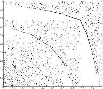
Example 2.3 shows that discrete measures $\nu$ give rise to $S^{-1}$ having (piecewise constant) closed form. As an example, scatter plots for the bivariate reciprocal Archimedean copula associated with the generator $F(t)=\exp(-\Lambda(t))$, for $\Lambda$ in (4), are depicted in Figure 1. From our simulations, it appears as though the resulting family converges to the independence copula for $\theta\rightarrow\infty$, and to some limiting copula (but not the upper Fréchet bound) for $\theta\rightarrow 0$. Furthermore, since $S^{-1}(t)=1/{\lceil t/\theta\rceil}$ maps to the discrete set $\{1/k\,:\,k\in\mathbb{N}\}$, the copula assigns positive mass to the one-dimensional subsets

$$A_{k}:=\Big{\{}\Big{(}F\Big{(}\frac{u}{k}\Big{)},F\Big{(}\frac{1-u}{k}\Big{)}\Big{)}\,:\,u\in(0,1)\Big{\}}\subset[0,1]^{2},\quad k\geq 1,$$

of the unit square. By construction, this mass is decreasing in $k$, and the first sets $A_{1},A_{2},\ldots$ are clearly visible in the scatter plots.

Fig. 1: Scatter plots for the bivariate reciprocal Archimedan copula with generator $F(t)=\exp(-\Lambda(t))$, for $\Lambda$ in (4). Left: $\theta=0.5$. Right: $\theta=0.025$.

In case $S^{-1}$ is not given in closed form, it is convenient to recall that $S$ is given in terms of $\Lambda$ by the Williamson transform inversion formula

$$S(t)=\sum_{k=0}^{d-2}\frac{(-1)^{k}\,\Lambda^{(k)}(t)}{k!}t^{k}+\frac{(-1)^{d-1}\,\Lambda^{(d-1)}_{+}(t)}{(d-1)!}(d-1)^{k},$$ (6)

with $\Lambda^{(d-1)}_{+}$ denoting the right-hand derivative of $\Lambda^{(d-2)}$, cf. [Genest et al. (2018)]. In particular, $\Lambda$ is $d$-monotone, which implies that the first $d-2$ derivatives exist, and $\Lambda^{(d-2)}$ is convex (so that $\Lambda^{(d-1)}_{+}$ exists). If $S$ has discontinuities, such as in the case of a discrete measure $\nu$ like in Example 2.3, $\Lambda$ is not $(d+1)$-monotone, i.e. $\Lambda^{(d-1)}$ does not exist. Besides traditional Newton-Raphson inversion, here are two more ideas for dealing with $S^{-1}$ in Algorithm 1:

• One idea to evaluate $S^{-1}$ approximatively is to approximate $S$ by a piecewise constant function, which amounts to approximation of $\nu$ by a discrete measure. Example 2.3 then gives the closed form of the resulting piecewise constant approximation to $S^{-1}$. This implies an approximative simulation algorithm for the reciprocal Archimedean copula in concern. In light of the relation between $S$ and $\Lambda$ in (6), this means that the exponent $\Lambda$ in concern is approximated by an exponent that is proper $d$-monotone, i.e. not $(d+1)$-monotone. Similarly, other invertible approximations might be feasible as well, for example a piecewise linear approximation of $S$. Notice that a piecewise constant approximation of a continuous survival function $S$ results in an approximating reciprocal Archimedean copula with singular component, while a piecewise linear approximation would not have this drawback.

• We assume that $S$ is differentiable. In step $n+1$ of the while-loop in Algorithm 1, the values $x_{n}:=\epsilon_{1}+\ldots+\epsilon_{n}$ and $S^{-1}(x_{n})$ have already been computed (in the previous step), and one seeks to simulate the random variable $S^{-1}(x_{n}+\epsilon_{n+1})$. In the initial step we have $x_{0}=0$ and $S^{-1}(0)=\infty$. The random variable $S^{-1}(x_{n}+\epsilon_{n+1})$ has density

  $$f(x):=e^{x_{n}}\,e^{-S(x)}\,S^{{}^{\prime}}(x),\quad x\in\big{(}0,S^{-1}(x_{n})\big{)},\quad n\geq 0,$$

  which is often given in closed form, e.g. by virtue of formula (6), so can be evaluated efficiently. If one can find a random variable $X$, which one can simulate from and whose density $g$ satisfies $f\leq c\,g$ for some $c\geq 1$, traditional rejection acceptance sampling can be applied, cf. [Mai, Scherer (2017), p. 235ff], which results in an exact simulation algorithm.

Remark 2.5 (Expected runtime in dependence on the dimension)

Using the stochastic representation (5) for the uniform distribution on the simplex, the simulation of the random vector $\mathbf{Q}^{(k)}$ in the $k$-th while-loop requires to simulate $d$ independent exponential random variables, hence has complexity order linear in $d$. However, the number of required while-loops is random itself. In the special case $\nu(\mathrm{d}x)=d\,x^{-2}\,\mathrm{d}x$, which corresponds to the Galambos copula with parameter $\theta=1$ and $S^{-1}(x)=d/x$, Algorithm 1 coincides with [Dombry et al. (2016), Algorithm 1]. [Dombry et al. (2016), Proposition 4], which in turn refers to [Oesting et al. (2018)], shows that the expected number of required while-loops in this case equals $\mathbb{E}[M]=d\,\mathbb{E}[\max\{X_{1},\ldots,X_{d}\}]$, where $(X_{1},\ldots,X_{d})$ is a random vector with survival copula the Galambos copula in concern and all one-dimensional margins unit exponentially distributed. It follows from a computation in [Mai (2014)] that

$$1\leq\mathbb{E}[\max\{X_{1},\ldots,X_{d}\}]=\sum_{i=1}^{d}\binom{d}{i}\,\frac{(-1)^{i+1}}{H_{i}}\leq d,$$

where $H_{n}:=1+1/2+\ldots+1/n$, $n=1,2,\ldots$, denotes the harmonic series. Hence, in this special case the complexity order of the algorithm is known explicitly as a function of the dimension $d$ and lies somewhere between $d^{2}$ and $d^{3}$. Unfortunately, the proof of this result relies heavily on the fact that $d/R_{k}=\epsilon_{1}+\ldots+\epsilon_{k}$. In the case of general radial measure, we have

$$\mathbb{E}[M] =1+\sum_{m=1}^{\infty}\mathbb{P}(M>m)=1+\sum_{m=1}^{\infty}\mathbb{P}(R_{k+1}>M_{k},\,k=1,\ldots,m)$$

$$=1+\sum_{m=1}^{\infty}\mathbb{P}\Big{(}\frac{S^{-1}\big{(}\sum_{i=1}^{m+1}\epsilon_{i}\big{)}}{S^{-1}\big{(}\sum_{i=1}^{k}\epsilon_{i}\big{)}}>\max\big{\{}Q^{(k)}_{1},\ldots,Q^{(k)}_{d}\big{\}},\,k=1,\ldots,m\Big{)}.$$

From this formula for $S^{-1}(x)=d/x$, [Oesting et al. (2018)] make use of the fact that $\sum_{i=1}^{k}\epsilon_{i}/\sum_{i=1}^{m+1}\epsilon_{i}$, for $k=1,\ldots,m$, correspond to order statistics of independent samples from the uniform law on $[0,1]$, which we cannot for general $\nu$ (hence $S^{-1}$). However, using this known Galambos case as benchmark, from the last formula we observe that $\mathbb{E}[M]$ is larger than in the known benchmark case if the function $x\mapsto S^{-1}(x)\,x$ is increasing, and that it is smaller if $x\mapsto S^{-1}(x)\,x$ is decreasing. Although we cannot say a lot about the case when $x\mapsto S^{-1}(x)\,x$ is neither increasing nor decreasing, this at least provides a feeling for the effect of the choice of radial measure on the expected runtime of the algorithm. In the case when $\nu$ is absolutely continuous with density $f_{\nu}$ one may check whether $x\mapsto S^{-1}(x)\,x$ is increasing (resp. decreasing) by checking whether $f_{\nu}(x)\,x\geq S(x)$ (resp. $f_{\nu}(x)\,x\leq S(x)$) for all $x>0$, which is a quite intuitive condition in terms of the density. Heuristically, it says that heavier tails of the radial measure make the algorithm faster, and vice versa.

3 Conclusion

An exact simulation algorithm for reciprocal Archimedean copulas has been presented. It was based on the concatenation of two ideas. On the one hand, via a change of variables transformation the points of a Poisson random measure on $(0,\infty]$, whose mean measure equals the radial measure of the reciprocal Archimedean copula, have been represented as a decreasing function of the jump times of a standard Poisson process. On the other hand, an idea of [Dombry et al. (2016)] has been enhanced from a simulation algorithm for extreme-value copulas to copulas of more general max-infinitely divisible distributions, of which reciprocal Archimedean copulas are a particular representative.

References

- [Bondesson (1982)] L. Bondesson, On simulation from infinitely divisible distributions, Advances in Applied Probability 14 (1982) pp. 855–869.
- [Dombry et al. (2016)] C. Dombry, S. Engelke, M. Oesting, Exact simulation of max-stable processes, Biometrika 103:2 (2016) pp. 303–317.
- [Fang et al. (1990)] K.-T. Fang, S. Kotz, K.-W. Ng, Symmetric multivariate and related distributions, Chapman and Hall, London (1990).
- [Galambos (1975)] J. Galambos, Order statistics of samples from multivariate distributions, Journal of the American Statistical Association 70:351 (1975) pp. 674–680.
- [Genest et al. (2018)] C. Genest, J. Nešlehová, L.-P. Rivest, The class of multivariate max-id copulas with -norm symmetric exponent measures, Bernoulli, in press (2018).
- [Mai (2014)] J.-F. Mai, A note on the Galambos copula and its associated Bernstein function, Dependence Modeling 2 (2014) pp. 22–29.
- [Mai, Scherer (2017)] J.-F. Mai, M. Scherer, Simulating Copulas, 2nd edition, World Scientific Press (2017).
- [McNeil, Nešlehová (2009)] A.J. McNeil, J. Nešlehová, Multivariate Archimedean copulas, -monotone functions and -norm symmetric distributions, Annals of Statistics 37:5B (2009) pp. 3059–3097.
- [Nelsen (2006)] R.B. Nelsen, An introduction to copulas, 2nd edition, Springer (2006).
- [Oesting et al. (2018)] M. Oesting, M. Schlather, C. Zhou, Exact and fast simulation of max-stable processes on a compact set using the normalized spectral representation, Bernoulli 24:1 (2018), pp. 1497–1530.
- [Resnick (1987)] S. Resnick, Extreme values, regular variation and point processes, Springer-Verlag (1987).
- [Schlather (2002)] M. Schlather, Models for stationary max-stable random fields, Extremes 5:1 (2002), pp. 33–44.