Abstract

Many applications, including rank aggregation and crowd-labeling, can be modeled in terms of a bivariate isotonic matrix with unknown permutations acting on its rows and columns. We consider the problem of estimating such a matrix based on noisy observations of a subset of its entries, and design and analyze a polynomial-time algorithm that improves upon the state of the art. In particular, our results imply that any such $n\times n$ matrix can be estimated efficiently in the normalized Frobenius norm at rate $\widetilde{\mathcal{O}}(n^{-3/4})$, thus narrowing the gap between $\widetilde{\mathcal{O}}(n^{-1})$ and $\widetilde{\mathcal{O}}(n^{-1/2})$, which were hitherto the rates of the most statistically and computationally efficient methods, respectively.

1 Introduction

Structured matrices with entries in the range $[0,1]$ and unknown permutations acting on their rows and columns arise in multiple applications, including estimation from pairwise comparisons [BT52, SBGW17] and crowd-labeling [DS79, SBW16b]. Traditional parametric models [BT52, Luc59, Thu27, DS79] assume that these matrices are obtained from rank-one matrices via a known link function. Aided by tools such as maximum likelihood estimation and spectral methods, researchers have made significant progress in studying both statistical and computational aspects of these parametric models [HOX14, RA14, SBB⁺16, NOS16, ZCZJ16, GZ13, GLZ16, KOS11b, LPI12, DDKR13, GKM11] and their low-rank generalizations [RA16, NOTX17, KOS11a].

There has been evidence from empirical studies (e.g., [ML65, BW97]) that real-world data is not always well-captured by such parametric models. With the goal of increasing model flexibility, a recent line of work has studied the class of permutation-based models [Cha15, SBGW17, SBW16b]. Rather than imposing parametric conditions on the matrix entries, these models impose only shape constraints on the matrix, such as monotonicity, before unknown permutations act on the its rows and columns. This more flexible class reduces modeling bias compared to its parametric counterparts while, perhaps surprisingly, producing models that can be estimated at rates that differ only by logarithmic factors from parametric models. On the negative side, these advantages of permutation-based models are accompanied by significant computational challenges. The unknown permutations make the parameter space highly non-convex, so that efficient maximum likelihood estimation is unlikely. Moreover, spectral methods are often suboptimal in approximating shape-constrained sets of matrices [Cha15, SBGW17]. Consequently, results from many recent papers show a non-trivial statistical-computational gap in estimation rates for models with latent permutations [SBGW17, CM16, SBW16b, FMR16, PWC17].

Related work.

While the main motivation of our work comes from nonparametric methods for aggregating pairwise comparisons, we begin by discussing a few other lines of related work. The current paper lies at the intersection of shape-constrained estimation and latent permutation learning. Shape-constrained estimation has long been a major topic in nonparametric statistics, and of particular relevance to our work is the estimation of a bivariate isotonic matrix without latent permutations [CGS18]. There, it was shown that the minimax rate of estimating an $n\times n$ matrix from noisy observations of all its entries is $\widetilde{\Theta}(n^{-1})$. The upper bound is achieved by the least squares estimator, which is efficiently computable due to the convexity of the parameter space.

Shape-constrained matrices with permuted rows or columns also arise in applications such as seriation [FJBd13, FMR16] and feature matching [CD16]. In particular, the monotone subclass of the statistical seriation model [FMR16] contains $n\times n$ matrices that have increasing columns, and an unknown row permutation. The authors established the minimax rate $\widetilde{\Theta}(n^{-2/3})$ for estimating matrices in this class and proposed a computationally efficient algorithm with rate $\widetilde{\mathcal{O}}(n^{-1/2})$. For the subclass of such matrices where in addition, the rows are also monotone, the results of the current paper improve the two rates to $\widetilde{\mathcal{O}}(n^{-1})$ and $\widetilde{\mathcal{O}}(n^{-3/4})$ respectively.

Another related model is that of noisy sorting [BM08], which involves a latent permutation but no shape-constraint. In this prototype of a permutation-based ranking model, we have an unknown, $n\times n$ matrix with constant upper and lower triangular portions whose rows and columns are acted upon by an unknown permutation. The hardness of recovering any such matrix in noise lies in estimating the unknown permutation. As it turns out, this class of matrices can be estimated efficiently at minimax optimal rate $\widetilde{\Theta}(n^{-1})$ by multiple procedures: the original work by Braverman and Mossel [BM08] proposed an algorithm with time complexity $\mathcal{O}(n^{c})$ for some unknown and large constant $c$, and recently, an $\widetilde{\mathcal{O}}(n^{2})$-time algorithm was proposed by Mao et al. [MWR17]. These algorithms, however, do not generalize beyond the noisy sorting class, which constitutes a small subclass of an interesting class of matrices that we describe next.

The most relevant body of work to the current paper is that on estimating matrices satisfying the strong stochastic transitivity condition, or SST for short. This class of matrices contains all $n\times n$ bivariate isotonic matrices with unknown permutations acting on their rows and columns, with an additional skew-symmetry constraint. The first theoretical study of these matrices was carried out by Chatterjee [Cha15], who showed that a spectral algorithm achieved the rate $\widetilde{\mathcal{O}}(n^{-1/4})$ in the normalized Frobenius norm. Shah et al. [SBGW17] then showed that the minimax rate of estimation is given by $\widetilde{\Theta}(n^{-1})$, and also improved the analysis of the spectral estimator of Chatterjee [Cha15] to obtain the computationally efficient rate $\widetilde{\mathcal{O}}(n^{-1/2})$. In follow-up work [SBW16a], they also showed a second $\mathsf{CRL}$ estimator based on the Borda count that achieved the same rate, but in near-linear time. In related work, Chatterjee and Mukherjee [CM16] analyzed a variant of the $\mathsf{CRL}$ estimator, showing that for subclasses of SST matrices, it achieved rates that were faster than $\mathcal{O}(n^{-1/2})$. In a complementary direction, a superset of the current authors [PMM⁺17] analyzed the estimation problem under an observation model with structured missing data, and showed that for many observation patterns, a variant of the $\mathsf{CRL}$ estimator was minimax optimal.

Shah et al. [SBW16a] also showed that conditioned on the planted clique conjecture, it is impossible to improve upon a certain notion of adaptivity of the $\mathsf{CRL}$ estimator in polynomial time. Such results have prompted various authors [FMR16, SBW16a] to conjecture that a similar statistical-computational gap also exists when estimating SST matrices in the Frobenius norm.

Our contributions.

Our main contribution in the current work is to tighten the aforementioned statistical-computational gap. More precisely, we study the problem of estimating a bivariate isotonic matrix with unknown permutations acting on its rows and columns, given noisy, partial observations of its entries; this matrix class strictly contains the SST model [Cha15, SBGW17] for ranking from pairwise comparisons. As a corollary of our results, we show that when the underlying matrix has dimension $n\times n$ and $\Theta(n^{2})$ noisy entries are observed, our polynomial-time, two-dimensional sorting algorithm provably achieves the rate of estimation $\widetilde{}\mathcal{O}(n^{-3/4})$ in the normalized Frobenius norm; thus, this result breaks the previously mentioned $\widetilde{}\mathcal{O}(n^{-1/2})$ barrier [SBGW17, CM16]. Although the rate $\widetilde{}\mathcal{O}(n^{-3/4})$ still differs from the minimax optimal rate $\widetilde{\Theta}(n^{-1})$, our algorithm is, to the best of our knowledge, the first efficient procedure to obtain a rate faster than $\widetilde{}\mathcal{O}(n^{-1/2})$ uniformly over the SST class. This guarantee, which is stated in slightly more technical terms below, can be significant in practice (see Figure 1).

Main theorem (informal)

There is an estimator $\widehat{M}$ computable in time $\mathcal{O}(n^{2.5})$ such that for any $n\times n$ SST matrix $M^{*}$, given $\Theta(n^{2})$ Bernoulli observations of its entries, we have

$$\mathbb{E}\left[\frac{1}{n^{2}}\|\widehat{M}-M^{*}\|_{F}^{2}\right]\leq C\left(\frac{\log n}{n}\right)^{3/4}.$$

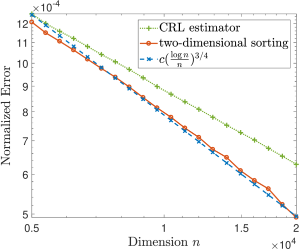
Figure 1: Left: A bivariate isotonic matrix; $M^{*}\in[0,1]^{n\times n}$ is a row and column permuted version of such a matrix. Right: A log-log plot of the error $\frac{1}{n^{2}}\|\widehat{M}-M^{*}\|_{F}^{2}$ (averaged over $10$ experiments each using $n^{2}$ Bernoulli observations) of our estimator and the $\mathsf{CRL}$ estimator [SBW16a].

Our algorithm is novel in the sense that it is neither spectral in nature, nor simple variations of the Borda count estimator that was previously employed. Our algorithm takes advantage of the fine monotonicity structure of the underlying matrix along both dimensions, and this allows us to prove tighter bounds than before. In addition to making algorithmic contributions, we also briefly revisit the minimax rates of estimation.

Organization.

In Section 2, we formally introduce our estimation problem. Section 3 contains statements and discussions of our main results, and in Section 4, we describe in detail how the estimation problem that we study is connected to applications in crowd-labeling and ranking from pairwise comparisons. We provide the proofs of our main results in Section 5.

Notation.

For a positive integer $n$, let $[n]:\,=\{1,2,\ldots,n\}$. For a finite set $S$, we use $|S|$ to denote its cardinality. For two sequences $\{a_{n}\}_{n=1}^{\infty}$ and $\{b_{n}\}_{n=1}^{\infty}$, we write $a_{n}\lesssim b_{n}$ if there is a universal constant $C$ such that $a_{n}\leq Cb_{n}$ for all $n\geq 1$. The relation $a_{n}\gtrsim b_{n}$ is defined analogously. We use $c,C,c_{1},c_{2},\dots$ to denote universal constants that may change from line to line. We use $\mbox{\sf Ber}(p)$ to denote the Bernoulli distribution with success probability $p$, the notation $\mbox{\sf Bin}(n,p)$ to denote the binomial distribution with $n$ trials and success probability $p$, and the notation $\operatorname{\mathsf{Poi}}(\lambda)$ to denote the Poisson distribution with parameter $\lambda$. Given a matrix $M\in{}^{n_{1}\times n_{2}}$, its $i$-th row is denoted by $M_{i}$. For a vector $v\in\mathbb{R}^{n}$, define its variation as $\operatorname{\mathsf{var}}(v)=\max_{i}v_{i}-\min_{i}v_{i}$. Let $\mathfrak{S}_{n}$ denote the set of all permutations $\pi:[n]\to[n]$. Let $\mathsf{id}$ denote the identity permutation, where the dimension can be inferred from context.

2 Background and problem setup

In this section, we present the relevant technical background and notation on permutation-based models, and introduce the observation model of interest.

2.1 Matrix models

Our main focus is on designing efficient algorithms for estimating a bivariate isotonic matrix with unknown permutations acting on its rows and columns. Formally, we define $\mathbb{C}_{\mathsf{BISO}}$ to be the class of matrices in $[0,1]^{n_{1}\times n_{2}}$ with nondecreasing rows and nondecreasing columns. For readability, we assume throughout that $n_{1}\geq n_{2}$ unless otherwise stated; our results can be straightforwardly extended to the other case. Given a matrix $M\in{}^{n_{1}\times n_{2}}$ and permutations $\pi\in\mathfrak{S}_{n_{1}}$ and $\sigma\in\mathfrak{S}_{n_{2}}$, we define the matrix $M(\pi,\sigma)\in{}^{n_{1}\times n_{2}}$ by specifying its entries as

$$\left[M(\pi,\sigma)\right]_{i,j}=M_{\pi(i),\sigma(j)}\text{ for }i\in[n_{1}],j\in[n_{2}].$$

Also define the class $\mathbb{C}_{\mathsf{BISO}}(\pi,\sigma):\,=\{M(\pi,\sigma):M\in\mathbb{C}_{\mathsf{BISO}}\}$ as the set of matrices that are bivariate isotonic when viewed along the row permutation $\pi$ and column permutation $\sigma$, respectively.

The class of matrices that we are interested in estimating contains bivariate isotonic matrices whose rows and columns are both acted upon by unknown permutations:

$$\mathbb{C}_{\mathsf{Perm}}:\,=\bigcup_{\begin{subarray}{c}\pi\in\mathfrak{S}_{n_{1}}\\ \sigma\in\mathfrak{S}_{n_{2}}\end{subarray}}\mathbb{C}_{\mathsf{BISO}}(\pi,\sigma).$$

2.2 Observation model

In order to study estimation from noisy observations of a matrix $M^{*}$ in the class $\mathbb{C}_{\mathsf{Perm}}$, we suppose that $N$ noisy entries are sampled independently and uniformly with replacement from all entries of $M^{*}$. This sampling model is popular in the matrix completion literature, and is a special case of the trace regression model [NW12, KLT11]. It has also been used in the context of permutation models by Mao et al. [MWR17] to study the noisy sorting class.

More precisely, let $E^{(i,j)}$ denote the $n_{1}\times n_{2}$ matrix with $1$ in the $(i,j)$-th entry and $0$ elsewhere, and suppose that $X_{\ell}$ is a random matrix sampled independently and uniformly from the set $\{E^{(i,j)}:i\in[n_{1}],\,j\in[n_{2}]\}$. We observe $N\leq n_{1}n_{2}$ independent pairs $\{(X_{\ell},y_{\ell})\}_{\ell=1}^{N}$ from the model

$$y_{\ell}=\operatorname{\mathsf{tr}}(X_{\ell}^{\top}M^{*})+z_{\ell},$$ (1)

where the observations are contaminated by independent, centered, sub-Gaussian noise $z_{\ell}$ with variance parameter $\zeta^{2}$. Of particular interest is the noise model considered in applications such as crowd-labeling and ranking from pairwise comparisons. Here our samples take the form

$$y_{\ell}\sim\mbox{\sf Ber}\big{(}\operatorname{\mathsf{tr}}(X_{\ell}^{\top}M)\big{)}$$ (2)

and consequently, the sub-Gaussian parameter $\zeta^{2}$ is bounded; for a discussion of other regimes of noise in a related matrix model, see Gao [Gao17].

For analytical convenience, we employ the standard trick of Poissonization, whereby we assume throughout the paper that $N^{\prime}=\operatorname{\mathsf{Poi}}(N)$ random samples are drawn according to the trace regression model (1). Upper and lower bounds derived under this model carry over with loss of constant factors to the model with exactly $N$ samples; for a detailed discussion, see Appendix B.

For notational convenience, denote the probability that an entry of the matrix is observed under Poissonized sampling by $p_{\mathsf{obs}}=1-\exp(-N/n_{1}n_{2})$. Since we assume throughout that $N\leq n_{1}n_{2}$, it can be verified that $\frac{N}{2n_{1}n_{2}}\leq p_{\mathsf{obs}}\leq\frac{N}{n_{1}n_{2}}$.

Now given $N^{\prime}=\operatorname{\mathsf{Poi}}(N)$ observations $\{(X_{\ell},y_{\ell})\}_{\ell=1}^{N^{\prime}}$, let us define the matrix of observations $Y=Y\left(\{(X_{\ell},y_{\ell})\}_{\ell=1}^{N^{\prime}}\right)$, with entry $(i,j)$ given by

$$Y_{i,j}=\frac{1}{p_{\mathsf{obs}}}\frac{1}{1\vee\sum_{\ell=1}^{N^{\prime}}\mathbf{1}\{X_{\ell}=E^{(i,j)}\}}\sum_{\ell=1}^{N^{\prime}}y_{\ell}\,\mathbf{1}\{X_{\ell}=E^{(i,j)}\}.$$ (3)

In words, the rescaled entry $p_{\mathsf{obs}}Y_{i,j}$ is the average of all the noisy realizations of $M^{*}_{i,j}$ that we have observed, or zero if the entry goes unobserved. Note that $\mathbb{E}[Y_{i,j}]=\frac{1}{p_{\mathsf{obs}}}M^{*}_{i,j}\cdot p_{\mathsf{obs}}=M^{*}_{i,j},$ so that ${\mathbb{E}}[Y]=M^{*}$. Moreover, we may write the model in the linearized form $Y=M^{*}+W$, where $W$ is a matrix of additive noise having independent, zero-mean, sub-Gaussian entries.

3 Main results

In this section, we present our main results—we begin by briefly revisiting the fundamental limits of estimation, and then introduce our algorithms in Section 3.2. We assume throughout this section that as per the setup, we have $n_{1}\geq n_{2}$ and $N\in[n_{1}n_{2}]$.

3.1 Statistical limits of estimation

We begin by characterizing the fundamental limits of estimation under the trace regression observation model (1) with $N^{\prime}=\operatorname{\mathsf{Poi}}(N)$ observations. We define the least squares estimator over the class of matrices $\mathbb{C}_{\mathsf{Perm}}$ as the projection

$$\widehat{M}_{{\sf LS}}(Y):\,=\arg\min_{M\in\mathbb{C}_{\mathsf{Perm}}}\|Y-M\|_{F}^{2}.$$

The projection is a non-convex problem, and is unlikely to be computable exactly in polynomial time. However, studying this estimator allows us to establish a baseline that characterizes the best achievable statistical rate. The following theorem characterizes its risk up to a logarithmic factor in the dimension; recall the shorthand $Y=Y\left(\{X_{\ell},y_{\ell}\}_{\ell=1}^{N^{\prime}}\right)$.

Theorem 1.

For any matrix $M^{*}\in\mathbb{C}_{\mathsf{Perm}}$, we have

$$\frac{1}{n_{1}n_{2}}\|\widehat{M}_{{\sf LS}}(Y)-M^{*}\|_{F}^{2}\lesssim(\zeta^{2}\lor 1)\frac{n_{1}\log^{2}n_{1}}{N}$$ (4a)

with probability at least $$1-(n_{1}n_{2})^{-3}$$.

Additionally, under the Bernoulli observation model (2), any estimator $\widehat{M}$ satisfies

$$\sup_{M^{*}\in\mathbb{C}_{\mathsf{Perm}}}\mathbb{E}\left[\frac{1}{n_{1}n_{2}}\|\widehat{M}-M^{*}\|_{F}^{2}\right]\gtrsim\frac{n_{1}}{N}.$$ (4b)

The factor $(\zeta^{2}\lor 1)$ appears in the upper bound instead of the noise variance $\zeta^{2}$ because even if the noise is zero, there are missing entries. The theorem characterizes the minimax rate of estimation for the class $\mathbb{C}_{\mathsf{Perm}}$ up to a logarithmic factor.

3.2 Efficient algorithms

Next, we propose polynomial-time algorithms for estimating the permutations $(\pi,\sigma)$ and the matrix $M^{*}$. Our main algorithm relies on two distinct steps: first, we estimate the unknown permutations, and then project onto the class of matrices that are bivariate isotonic when viewed along the estimated permutations. The formal meta-algorithm is described below.

Algorithm 1 (meta-algorithm)

• Step 0: Split the observations into two disjoint parts, each containing $N^{\prime}/2$ observations, and construct the matrices $Y^{(1)}=Y\left(\{X_{\ell},y_{\ell}\}_{\ell=1}^{N^{\prime}/2}\right)$ and $Y^{(2)}=Y\left(\{X_{\ell},y_{\ell}\}_{\ell=N^{\prime}/2+1}^{N^{\prime}}\right)$.

• Step 1: Use $Y^{(1)}$ to obtain the permutation estimates $(\widehat{\pi},\widehat{\sigma})$.

• Step 2: Return the matrix estimate $\widehat{M}(\widehat{\pi},\widehat{\sigma}):\,=\arg\min_{M\in\mathbb{C}_{\mathsf{BISO}}(\widehat{\pi},\widehat{\sigma})}\|Y^{(2)}-M\|_{F}^{2}.$

Owing to the convexity of the set $\mathbb{C}_{\mathsf{BISO}}(\widehat{\pi},\widehat{\sigma})$, the projection operation in Step 2 of the algorithm can be computed in near linear time [BDPR84, KRS15]. The following result, a slight variant of Proposition 4.2 of Chatterjee and Mukherjee [CM16], allows us to characterize the error rate of any such meta-algorithm as a function of the permutation estimates $(\widehat{\pi},\widehat{\sigma})$.

Proposition 1.

Suppose that $M^{*}\in\mathbb{C}_{\mathsf{BISO}}(\pi,\sigma)$ where $\pi$ and $\sigma$ are unknown permutations in $\mathfrak{S}_{n_{1}}$ and $\mathfrak{S}_{n_{2}}$ respectively. Then with probability at least $1-(n_{1}n_{2})^{-3}$, we have

$$\frac{1}{n_{1}n_{2}}\big{\|}\widehat{M}(\widehat{\pi},\widehat{\sigma})-M^{*}\big{\|}_{F}^{2}\lesssim(\zeta^{2}\lor 1)\frac{n_{1}\log^{2}n_{1}}{N} +\frac{1}{n_{1}n_{2}}\big{\|}M^{*}(\pi^{-1}\circ\widehat{\pi},\mathsf{id})-M^{*}\big{\|}_{F}^{2}$$

$$+\frac{1}{n_{1}n_{2}}\big{\|}M^{*}(\mathsf{id},\sigma^{-1}\circ\widehat{\sigma})-M^{*}\big{\|}_{F}^{2}.$$ (5)

The first term on the right hand side of the bound (5) corresponds to an estimation error, if the true permutations $\pi$ and $\sigma$ were known a priori, and the latter two terms correspond to an approximation error that we incur as a result of having to estimate these permutations from data. Comparing the bound (5) to the minimax lower bound (4b), we see that up to a logarithmic factor, the first term of the bound (5) is unavoidable, and so we can restrict our attention to obtaining good permutation estimates $(\widehat{\pi},\widehat{\sigma})$. We now present our main permutation estimation procedure that can be plugged into Step 1 of this meta-algorithm.

3.2.1 Two-dimensional sorting

Since the underlying matrix of interest is individually monotonic along each dimension, the row and column sums provide noisy information about the respective unknown permutations. Consequently, variants of such procedures are popular in the literature [CM16, FMR16]. However, such a procedure does not take simultaneous advantage of the fact that the underlying matrix is monotonic in both dimensions. To improve upon simply sorting row (resp. column) sums, we propose an algorithm that first sorts the columns (resp. rows) of the matrix approximately, and then exploits this approximate ordering to sort the rows (resp. columns) of the matrix.

We need more notation to facilitate the description of the algorithm. For a partition
$\mathsf{bl}=(\mathsf{bl}_{1},\dots,\mathsf{bl}_{K})$ of the set $[n_{2}]$, we group the columns of a matrix $Y\in{}^{n_{1}\times n_{2}}$ into $K$ blocks according to their indices in $\mathsf{bl}$, and refer to $\mathsf{bl}$ as a partition or blocking of the columns of $Y$.

Given a data matrix $Y\in{}^{n_{1}\times n_{2}}$, the following blocking subroutine returns a column partition $\mathsf{BL}(Y)$. In the main algorithm, partial row sums are computed on indices contained in each block.

Subroutine 1 (blocking)

• Step 1: Compute the column sums $\{C(j)\}_{j=1}^{n_{2}}$ of the matrix $Y$ as

  $$C(j)=\sum_{i=1}^{n_{1}}Y_{i,j}.$$

  Let $\widehat{\sigma}_{\sf pre}$ be the permutation along which the sequence $\{C(\widehat{\sigma}_{\sf pre}(j))\}_{j=1}^{n_{2}}$ is nondecreasing.

• Step 2: Set $\tau=16(\zeta+1)\Big{(}\sqrt{\frac{n_{1}^{2}n_{2}}{N}\log(n_{1}n_{2})}+\frac{n_{1}n_{2}}{N}\log(n_{1}n_{2})\Big{)}$ and $K=\lceil n_{2}/\tau\rceil$. Partition the columns of $Y$ into $K$ blocks by defining

  $$\mathsf{bl}_{1} =\{j\in[n_{2}]:C(j)\in(-\infty,\tau)\},$$

  $$\mathsf{bl}_{k} =\left\{j\in[n_{2}]:C(j)\in\big{[}(k-1)\tau,k\tau\big{)}\right\}\text{ for }1<k<K,\text{ and}$$

  $$\mathsf{bl}_{K} =\{j\in[n_{2}]:C(j)\in[(K-1)\tau,\infty)\}.$$

  Note that each block is contiguous when the columns are permuted by $\widehat{\sigma}_{\sf pre}$.

• Step 3 (aggregation): Set $\beta=n_{2}\sqrt{\frac{n_{1}}{N}\log(n_{1}n_{2})}$. Call a block $\mathsf{bl}_{k}$ “large” if $|\mathsf{bl}_{k}|\geq\beta$ and “small” otherwise. Aggregate small blocks in $\mathsf{bl}$ while leaving the large blocks as they are, to obtain the final partition $\mathsf{BL}$.

  More precisely, consider the matrix $Y^{\prime}=Y(\mathsf{id},\widehat{\sigma}_{\sf pre})$ having nondecreasing column sums and contiguous blocks. Call two small blocks “adjacent” if there is no other small block between them. Take unions of adjacent small blocks to ensure that the size of each resulting block is in the range $[\frac{1}{2}\beta,2\beta]$. If the union of all small blocks is smaller than $\frac{1}{2}\beta$, aggregate them all.

  Return the resulting partition $\mathsf{BL}(Y)=\mathsf{BL}$.

The threshold $\tau$ is a chosen to be a high probability bound on the perturbation of any column sum. In particular, this ensures that we obtain blocks containing columns that are close when the matrix is ordered according to the correct permutation. Computing partial row sums within each block then provides more refined information about the underlying row permutation than simply computing full row sums, and this intuition underlies the two-dimensional sorting algorithm to follow. As a technical detail, it is important to note that Step 3 aggregates small blocks into large enough ones to reduce noise in these partial row sums. We are now in a position to describe the two-dimensional sorting algorithm.

Algorithm 2 (two-dimensional sorting)

• Step 0: Split the observations into two independent subsamples of equal size, and form the corresponding matrices $Y^{(1)}$ and $Y^{(2)}$ according to equation (3).

• Step 1: Apply Subroutine 1 to the matrix $Y^{(1)}$ to obtain a partition $\mathsf{BL}=\mathsf{BL}(Y^{(1)})$ of the columns. Let $K$ be the number of blocks in $\mathsf{BL}$.

• Step 2: Using the second sample $Y^{(2)}$, compute the row sums

  $$S(i)=\sum_{j\in[n_{2}]}Y^{(2)}_{i,j}\text{ for each }i\in[n_{1}],$$

  and the partial row sums within each block

  $$S_{\mathsf{BL}_{k}}(i)=\sum_{j\in\mathsf{BL}_{k}}Y^{(2)}_{i,j}\text{ for each }i\in[n_{1}],k\in[K].$$

  Create a directed graph $G$ with vertex set $[n_{1}]$, where an edge $u\to v$ is present if either

  $$S(v)-S(u) >16(\zeta+1)\bigg{(}\sqrt{\frac{n_{1}n_{2}^{2}}{N}\log(n_{1}n_{2})}+\frac{n_{1}n_{2}}{N}\log(n_{1}n_{2})\bigg{)},\text{ or}$$ (6a)

  $$S_{\mathsf{BL}_{k}}(v)-S_{\mathsf{BL}_{k}}(u) >16(\zeta+1)\bigg{(}\sqrt{\frac{n_{1}n_{2}}{N}|\mathsf{BL}_{k}|\log(n_{1}n_{2})}+\frac{n_{1}n_{2}}{N}\log(n_{1}n_{2})\bigg{)}\text{ for some }k\in[K].$$ (6b)

• Step 3: Compute a topological sort $\widehat{\pi}_{\sf tds}$ of the graph $G$; if none exists, set $\widehat{\pi}_{\sf tds}=\mathsf{id}$.

• Step 4: Repeat Steps 1–3 with $(Y^{(i)})^{\top}$ replacing $Y^{(i)}$ for $i=1,2$, the roles of $n_{1}$ and $n_{2}$ switched, and the roles of $\pi$ and $\sigma$ switched, to compute the permutation estimate $\widehat{\sigma}_{\sf tds}$.

• Step 5: Return the permutation estimates $(\widehat{\pi}_{\sf tds},\widehat{\sigma}_{\sf tds})$.

Recall that a permutation $\pi$ is called a topological sort of $G$ if $\pi(u)<\pi(v)$ for every directed edge $u\to v$. The construction of the graph $G$ in Step 2 dominates the computational complexity, and takes time $\mathcal{O}(n_{1}^{2}n_{2}/\beta)=\mathcal{O}(n_{1}^{2}n_{2}^{1/2})$. We have the following guarantee for the two-dimensional sorting algorithm.

Theorem 2.

For any matrix $M^{*}\in\mathbb{C}_{\mathsf{Perm}}$, we have

$$\frac{1}{n_{1}n_{2}}\big{\|}\widehat{M}(\widehat{\pi}_{\sf tds},\widehat{\sigma}_{\sf tds})-M^{*}\big{\|}_{F}^{2}\lesssim(\zeta^{2}\lor 1)\left[\Big{(}\frac{n_{1}\log n_{1}}{N}\Big{)}^{3/4}+\frac{n_{1}\log^{2}n_{1}}{N}\right]$$

with probability at least $1-9(n_{1}n_{2})^{-3}$.

In particular, setting $N=n_{1}n_{2}$, we have proved that our efficient estimator enjoys the rate

$$\frac{1}{n_{1}n_{2}}\big{\|}\widehat{M}(\widehat{\pi}_{\sf tds},\widehat{\sigma}_{\sf tds})-M^{*}\big{\|}_{F}^{2}=\widetilde{O}\left(n_{2}^{-3/4}\right),$$

which is the main theoretical guarantee established in this paper for permutation-based models.

4 Applications

We now discuss in detail how the matrix models studied in this paper arise in practice. The class $\mathbb{C}_{\mathsf{Perm}}$ was studied as a permutation-based model for crowd-labeling [SBW16b] in the case of binary questions, and was proposed as a strict generalization of the classical Dawid-Skene model [DS79, KOS11b, LPI12, DDKR13, GKM11]. Here there is a set of $n_{2}$ questions of a binary nature; the true answer to these questions can be represented by a vector $x^{*}\in\{0,1\}^{n_{2}}$, and our goal is to estimate this vector by asking these questions to $n_{1}$ workers on a crowdsourcing platform. A key to this problem is being able to model the probabilities with which workers answer questions correctly, and we do so by collecting these probabilities within a matrix $M^{*}\in[0,1]^{n_{1}\times n_{2}}$. Assuming that workers have a strict ordering $\pi$ of their abilities, and that questions have a strict ordering $\sigma$ of their difficulties, the matrix $M^{*}$ is bivariate isotonic when the rows are ordered in increasing order of worker ability, and columns are ordered in decreasing order of question difficulty. However, since worker abilities and question difficulties are unknown a priori, the matrix of probabilities obeys the inclusion $M^{*}\in\mathbb{C}_{\mathsf{Perm}}$.

In the calibration problem, we would like to ask questions whose answers we know a priori, so that we can estimate worker abilities and question difficulties, or more generally, the entries of the matrix $M^{*}$. This corresponds to estimating matrices in the class $\mathbb{C}_{\mathsf{Perm}}$ from noisy observations of their entries, whose rate of estimation is our main result.

A subclass of $\mathbb{C}_{\mathsf{Perm}}$ specializes to the case $n_{1}=n_{2}=n$, and also imposes an additional skew symmetry constraint. More precisely, define $\mathbb{C}_{\mathsf{BISO}}^{\prime}$ analogously to the class $\mathbb{C}_{\mathsf{BISO}}$, except with matrices having columns that are nonincreasing instead of nondecreasing. Also define the class $\mathbb{C}_{\mathsf{skew}}(n):\,=\{M\in[0,1]^{n_{1}\times n_{2}}:M+M^{\top}=11^{\top}\}$, and the strong stochastic transitivity class

$$\mathbb{C}_{\mathsf{SST}}(n):\,=\left(\bigcup_{\pi\in\mathfrak{S}_{n}}\mathbb{C}_{\mathsf{BISO}}^{\prime}(\pi,\pi)\right)\bigcap\mathbb{C}_{\mathsf{skew}}(n).$$

The class $\mathbb{C}_{\mathsf{SST}}(n)$ is useful as a model for estimation from pairwise comparisons [Cha15, SBGW17], and was proposed as a strict generalization of parametric models for this problem [BT52, NOS16, RA14]. In particular, given $n$ items obeying some unknown underlying ranking $\pi$, entry $(i,j)$ of a matrix $M^{*}\in\mathbb{C}_{\mathsf{SST}}(n)$ represents the probability $\Pr(i\succ j)$ with which item $i$ beats item $j$ in a pairwise comparison between them. The shape constraint encodes the transitivity condition that for all triples $(i,j,k)$ obeying $\pi(i)<\pi(j)<\pi(k)$, we must have

$$\Pr(i\succ k)\geq\max\{\Pr(i\succ j),\Pr(j\succ k)\}.$$

For a more classical introduction to these models, see the papers [Fis73, ML65, BW97] and the references therein. Our task is to estimate the underlying ranking from results of passively chosen pairwise comparisons between the $n$ items, or more generally, to estimate the underlying probabilities $M^{*}$ that govern these comparisons. All the results we obtain in this work clearly extend to the class $\mathbb{C}_{\mathsf{SST}}(n)$ with minimal modifications; for example, either of the two estimates $\widehat{\pi}_{\sf tds}$ or $\widehat{\sigma}_{\sf tds}$ may be returned as an estimate of the permutation $\pi$. Consequently, the informal theorem stated in the introduction is an immediate corollary of Theorem 2 once these modifications are made to the algorithm.

5 Proofs

Throughout the proofs, we assume without loss of generality that $M^{*}\in\mathbb{C}_{\mathsf{BISO}}(\mathsf{id},\mathsf{id})=\mathbb{C}_{\mathsf{BISO}}$. Because we are interested in rates of estimation up to universal constants, we assume that each independent subsample contains $N^{\prime}=\operatorname{\mathsf{Poi}}(N)$ observations (instead of $\operatorname{\mathsf{Poi}}(N)/2$ or $\operatorname{\mathsf{Poi}}(N)/4$). We use the shorthand $Y=Y\left(\{(X_{\ell},y_{\ell})\}_{\ell=1}^{N^{\prime}}\right)$, throughout.

5.1 Some preliminary lemmas

Before turning to the proof of Theorems 1 and 2, we provide three lemmas that underlie many of our arguments. The first lemma can be readily distilled from the proof of Theorem 5 of Shah et al. [SBGW17] with slight modifications. It is worth mentioning that similar lemmas characterizing the estimation error of a bivariate isotonic matrix were also proved by [CGS18, CM16].

Lemma 1 ([SBGW17]).

Let $n_{1}\geq n_{2}$, and let $M^{*}\in\mathbb{C}_{\mathsf{Perm}}$. Assume that our observation model takes the form $Y=M^{*}+W$, where the noise matrix $W$ satisfies the properties

1. the entries $W_{i,j}$ are independent, centered, $\frac{c_{1}}{p_{\mathsf{obs}}}(\zeta\lor 1)$-sub-Gaussian random variables;

2. the second moments are bounded as ${\mathbb{E}}[|W_{i,j}|^{2}]\leq\frac{c_{2}}{p_{\mathsf{obs}}}(\zeta^{2}\lor 1)$ for all $i\in[n_{1}],j\in[n_{2}]$.

Then the least squares estimator $\widehat{M}_{{\sf LS}}(Y)$ satisfies

$$\Pr\left\{\Big{\|}\widehat{M}_{{\sf LS}}(Y)-M^{*}\Big{\|}_{F}^{2}\geq\frac{c_{3}}{p_{\mathsf{obs}}}(\zeta^{2}\lor 1)n_{1}\log^{2}n_{1}\right\}\leq(n_{1}n_{2})^{-3}.$$

Moreover, the same result holds if the class $\mathbb{C}_{\mathsf{Perm}}$ is replaced by the class $\mathbb{C}_{\mathsf{BISO}}$.

The proof closely follows that of Shah et al. [SBGW17, Theorem 5]; consequently, we postpone it to Appendix A. The next lemma establishes concentration of sums of our observations around their means.

Lemma 2.

For any nonempty subset $\mathcal{S}\subset[n_{1}]\times[n_{2}]$, it holds that

$$\Pr\left\{\bigg{|}\sum_{(i,j)\in\mathcal{S}}(Y_{i,j}-M^{*}_{i,j})\bigg{|}\geq 8(\zeta+1)\bigg{(}\sqrt{\frac{|\mathcal{S}|n_{1}n_{2}}{N}\log(n_{1}n_{2})}+2\frac{n_{1}n_{2}}{N}\log(n_{1}n_{2})\bigg{)}\right\}\leq 2(n_{1}n_{2})^{-4}.$$

Proof.

According to definitions (1) and (3), we have

$$W_{i,j}=Y_{i,j}-M^{*}_{i,j}=\begin{cases}-M^{*}_{i,j}\text{ if entry $(i,j)$ is not observed, and}\\ M^{*}_{i,j}/p_{\mathsf{obs}}-M^{*}_{i,j}+\frac{W^{\prime}_{i,j}}{p_{\mathsf{obs}}},\text{ otherwise,}\end{cases}$$

where $W^{\prime}$ is a $\zeta$-sub-Gaussian noise matrix with independent entries. Consequently, we can express the noise on each entry as $W_{i,j}=Z^{(1)}_{i,j}+Z^{(2)}_{i,j}$ where $\{Z^{(1)}_{i,j}\}_{i\in[n_{1}],j\in[n_{2}]}$ are independent, zero-mean random variables given by

$$Z^{(1)}_{i,j}=\begin{cases}M^{*}_{i,j}(p_{\mathsf{obs}}^{-1}-1)&\text{ with probability }p_{\mathsf{obs}},\\ -M^{*}_{i,j}&\text{ with probability }1-p_{\mathsf{obs}},\end{cases}$$

and $\{Z^{(2)}_{i,j}\}_{i\in[n_{1}],j\in[n_{2}]}$ are independent, zero-mean random variables such that

$$Z^{(2)}_{i,j}\text{ is }\begin{cases}\frac{\zeta}{p_{\mathsf{obs}}}\text{-sub-Gaussian}&\text{ with probability }p_{\mathsf{obs}},\\ 0&\text{ with probability }1-p_{\mathsf{obs}}.\end{cases}$$

We control the two separately. First, we have $|Z^{(1)}_{i,j}|\leq 1/p_{\mathsf{obs}}$ and the variance of each $Z^{(1)}_{i,j}$ is bounded by $(1-p_{\mathsf{obs}})^{2}/p_{\mathsf{obs}}+(1-p_{\mathsf{obs}})\leq 1/p_{\mathsf{obs}}$. Hence Bernstein’s inequality for bounded noise yields

$$\Pr\left\{\bigg{|}\sum_{(i,j)\in\mathcal{S}}Z^{(1)}_{i,j}\bigg{|}\geq t\right\}\leq 2\exp\Big{(}-\frac{t^{2}/2}{|\mathcal{S}|/p_{\mathsf{obs}}+t/(3p_{\mathsf{obs}})}\Big{)}.$$

Taking $t=4\sqrt{\frac{|\mathcal{S}|n_{1}n_{2}}{N}\log(n_{1}n_{2})}+6\frac{n_{1}n_{2}}{N}\log(n_{1}n_{2})$ and recalling that $p_{\mathsf{obs}}\geq\frac{N}{2n_{1}n_{2}}$, we obtain

$$\Pr\left\{\bigg{|}\sum_{(i,j)\in\mathcal{S}}Z^{(1)}_{i,j}\bigg{|}\geq 4\sqrt{\frac{|\mathcal{S}|n_{1}n_{2}}{N}\log(n_{1}n_{2})}+6\frac{n_{1}n_{2}}{N}\log(n_{1}n_{2})\right\}\leq(n_{1}n_{2})^{-4}.$$

In order to control the deviation of the sum of $Z^{(2)}_{i,j}$, we note that the $q$-th moment of $Z^{(2)}_{i,j}$ is bounded by $\frac{N}{n_{1}n_{2}}(\frac{2\zeta}{p_{\mathsf{obs}}}\sqrt{q})^{q}\leq\frac{q!}{2}\frac{8\zeta^{2}n_{1}n_{2}}{N}(\frac{4\zeta n_{1}n_{2}}{N})^{q-2}.$ Then another version of Bernstein’s inequality [BLM13] yields

$$\Pr\left\{\bigg{|}\sum_{(i,j)\in\mathcal{S}}Z^{(2)}_{i,j}\bigg{|}\geq\sqrt{\frac{16\zeta^{2}|\mathcal{S}|n_{1}n_{2}}{N}t}+\frac{4\zeta n_{1}n_{2}}{N}t\right\}\leq 2\exp(-t),$$

and setting $t=4\log(n_{1}n_{2})$ gives

$$\Pr\left\{\bigg{|}\sum_{(i,j)\in\mathcal{S}}Z^{(2)}_{i,j}\bigg{|}\geq 8\zeta\sqrt{\frac{|\mathcal{S}|n_{1}n_{2}}{N}\log(n_{1}n_{2})}+16\zeta\frac{n_{1}n_{2}}{N}\log(n_{1}n_{2})\right\}\leq(n_{1}n_{2})^{-4}.$$

Combining the above two deviation bounds completes the proof. ∎

The last lemma is a deterministic result.

Lemma 3.

Let $\{a_{i}\}_{i=1}^{n}$ be a nondecreasing sequence of real numbers. If $\pi$ is a permutation in $\mathfrak{S}_{n}$ such that $\pi(i)<\pi(j)$ whenever $a_{j}-a_{i}>\tau$ where $\tau>0$, then $|a_{\pi(i)}-a_{i}|\leq\tau$ for all $i\in[n]$.

Proof.

Suppose that $a_{j}-a_{\pi(j)}>\tau$ for some index $j\in[n]$. Since $\pi$ is a bijection, there must exist an index $i\leq\pi(j)$ such that $\pi(i)>\pi(j)$. However, we then have $a_{j}-a_{i}\geq a_{j}-a_{\pi(j)}>\tau$, which contradicts the assumption. A similar argument shows that $a_{\pi(j)}-a_{j}>\tau$ also leads to a contradiction. Therefore, we obtain that $|a_{\pi(j)}-a_{j}|\leq\tau$ for every $j\in[n]$. ∎

With these lemmas in hand, we are now ready to prove our main theorems.

5.2 Proof of Theorem 1

We split the proof into two parts by proving the upper and lower bounds separately.

5.2.1 Proof of upper bound

The upper bound follows from Lemma 1 once we check the conditions on the noise for our model. We have seen in the proof of Lemma 2 that the noise on each entry can be written as $W_{i,j}=Z^{(1)}_{i,j}+Z^{(2)}_{i,j}$. Again, $Z^{(1)}_{i,j}$ and $Z^{(2)}_{i,j}$ are $\frac{c}{p_{\mathsf{obs}}}$-sub-Gaussian and $\frac{c\,\zeta}{p_{\mathsf{obs}}}$-sub-Gaussian respectively, and have variances bounded by $\frac{1}{p_{\mathsf{obs}}}$ and $\frac{c\,\zeta^{2}}{p_{\mathsf{obs}}}$ respectively. Hence the conditions on $W$ in Lemma 1 are satisfied. Then we can apply the lemma, recall the relation $p_{\mathsf{obs}}\geq\frac{N}{2n_{1}n_{2}}$ and normalize the bound by $\frac{1}{n_{1}n_{2}}$ to complete the proof.

5.2.2 Proof of lower bound

The lower bound follows from an application of Fano’s lemma. The technique is standard, and we briefly review it here. Suppose we wish to estimate a parameter $\theta$ over an indexed class of distributions $\mathcal{P}=\{\mathbb{P}_{\theta}\,\mid\,\theta\in\Theta\}$ in the square of a (pseudo-)metric $\rho$. We refer to a subset of parameters $\{\theta^{1},\theta^{2},\ldots,\theta^{K}\}$ as a local $(\delta,\epsilon)$-packing set if

$$\min_{i,j\in[K],\,i\neq j}\rho(\theta^{i},\theta^{j})\geq\delta\qquad\text{ and }\qquad\frac{1}{K(K-1)}\sum_{i,j\in[K],\,i\neq j}D(\mathbb{P}_{\theta^{i}}\|\mathbb{P}_{\theta^{j}})\leq\epsilon.$$

Note that this set is a $\delta$-packing in the metric $\rho$ with the average KL-divergence bounded by $\epsilon$. The following result is a straightforward consequence of Fano’s inequality:

Lemma 4 (Local packing Fano lower bound).

For any $(\delta,\epsilon)$-packing set of cardinality $K$, we have

$$\inf_{\widehat{\theta}}\sup_{\theta^{*}\in\Theta}\mathbb{E}\left[\rho(\widehat{\theta},\theta^{*})^{2}\right]\geq\frac{\delta^{2}}{2}\left(1-\frac{\epsilon+\log 2}{\log K}\right).$$ (7)

In addition, the Gilbert-Varshamov bound [Gil52, Var57] guarantees the existence of binary vectors $\{v^{1},v^{2},\ldots,v^{K}\}\subseteq\{0,1\}^{n_{1}}$ such that

$$K \geq 2^{c_{1}n_{1}}\text{ and}$$ (8a)

$$\|v^{i}-v^{j}\|_{2}^{2} \geq c_{2}n_{1}\text{ for each }i\neq j,$$ (8b)

for some fixed tuple of constants $(c_{1},c_{2})$. We use this guarantee to design a packing of matrices in the class $\mathbb{C}_{\mathsf{Perm}}$. For each $i\in[K]$, fix some $\delta\in[0,1/4]$ to be precisely set later, and define the matrix $M^{i}$ having identical columns, with entries given by

$$M^{i}_{j,k}=\begin{cases}1/2,\text{ if }v^{i}_{j}=0\\ 1/2+\delta,\text{ otherwise.}\end{cases}$$ (9)

Clearly, each of these matrices $\{M^{i}\}_{i=1}^{K}$ is a member of the class $\mathbb{C}_{\mathsf{Perm}}$, and each distinct pair of matrices $(M^{i},M^{j})$ satisfies the inequality $\|M^{i}-M^{j}\|_{F}^{2}\geq c_{2}n_{1}n_{2}\delta^{2}$.

Let $\mathbb{P}_{M}$ denote the probability distribution of the observations in the model (2) with underlying matrix $M\in\mathbb{C}_{\mathsf{Perm}}$. Our observations are independent across entries of the matrix, and so the KL divergence tensorizes to yield

$$D(\mathbb{P}_{M^{i}}\|\mathbb{P}_{M^{j}})=\sum_{\begin{subarray}{c}k\in[n_{1}]\\ \ell\in[n_{2}]\end{subarray}}D(\mathbb{P}_{M^{i}_{k,\ell}}\|\mathbb{P}_{M^{j}_{k,\ell}}).$$

Let us now examine one term of this sum. We observe $T_{k,\ell}=\operatorname{\mathsf{Poi}}(\frac{N}{n_{1}n_{2}})$ samples of entry $(k,\ell)$; conditioned on the event $T_{k,\ell}=m$, we have the distributions

$$\mathbb{P}_{M^{i}_{k,\ell}}=\mbox{\sf Bin}(m,M^{i}_{k,\ell}),\quad\text{and}\quad\mathbb{P}_{M^{j}_{k,\ell}}=\mbox{\sf Bin}(m,M^{j}_{k,\ell}).$$

Consequently, the KL divergence conditioned on $T_{k,\ell}=m$ is given by

$$D(\mathbb{P}_{M^{i}_{k,\ell}}\|\mathbb{P}_{M^{j}_{k,\ell}})=mD(M^{i}_{k,\ell}\|M^{j}_{k,\ell}),$$

where we have used $D(p\|q)=p\log(\frac{p}{q})+(1-p)\log(\frac{1-p}{1-q})$ to denote the KL divergence between the Bernoulli random variables $\mbox{\sf Ber}(p)$ and $\mbox{\sf Ber}(q)$.

Note that for $p,q\in[1/2,3/4]$, we have

$$D(p\|q) =p\log\left(\frac{p}{q}\right)+(1-p)\log\left(\frac{1-p}{1-q}\right)$$

$$\stackrel{{\scriptstyle{\sf(i)}}}{{\leq}}p\left(\frac{p-q}{q}\right)+(1-p)\left(\frac{q-p}{1-q}\right)$$

$$=\frac{(p-q)^{2}}{q(1-q)}$$

$$\stackrel{{\scriptstyle{\sf(ii)}}}{{\leq}}\frac{16}{3}(p-q)^{2}.$$

Here, step ${\sf(i)}$ follows from the inequality $\log x\leq x-1$, and step ${\sf(ii)}$ from the assumption $q\in[\frac{1}{2},\frac{3}{4}]$. Taking the expectation with respect to $T_{k,\ell}$, we have

$$D(\mathbb{P}_{M^{i}_{k,\ell}}\|\mathbb{P}_{M^{j}_{k,\ell}})\leq\frac{16}{3}\frac{N}{n_{1}n_{2}}(M^{i}_{k,\ell}-M^{j}_{k,\ell})^{2}\leq\frac{16}{3}\frac{N}{n_{1}n_{2}}\delta^{2},$$

Summing over $k\in[n_{1}],\ell\in[n_{2}]$ yields $D(\mathbb{P}_{M^{i}}\|\mathbb{P}_{M^{j}})\leq\frac{16}{3}N\delta^{2}.$

Substituting into the Fano’s inequality (7), we have

$$\inf_{\widehat{M}}\sup_{M^{*}\in\mathbb{C}_{\mathsf{Perm}}}\mathbb{E}\left[\|\widehat{M}-M^{*}\|_{F}^{2}\right]\geq\frac{c_{2}n_{1}n_{2}\delta^{2}}{2}\left(1-\frac{\frac{16}{3}N\delta^{2}+\log 2}{c_{3}n_{1}}\right).$$

Finally, choosing $\delta^{2}=c\frac{n_{1}}{N}$ and normalizing by $n_{1}n_{2}$ yields the claim.

5.3 Proof of Proposition 1

Recall the definition of $\widehat{M}(\widehat{\pi},\widehat{\sigma})$ in the meta-algorithm, and additionally, define the projection of any matrix $M\in\mathbb{R}^{n_{1}\times n_{2}}$, as

$$\mathcal{P}_{\pi,\sigma}(M)=\arg\min_{\widetilde{M}\in\mathbb{C}_{\mathsf{BISO}}(\pi,\sigma)}\|M-\widetilde{M}\|_{F}^{2}.$$

and letting $W=Y^{(2)}-M^{*}$, we have

$$\|\widehat{M}(\widehat{\pi},\widehat{\sigma})-M^{*}\|_{F}^{2} \stackrel{{\scriptstyle{\sf(i)}}}{{\leq}}2\|\mathcal{P}_{\widehat{\pi},\widehat{\sigma}}(M^{*}+W)-\mathcal{P}_{\widehat{\pi},\widehat{\sigma}}(M^{*}(\widehat{\pi},\widehat{\sigma})+W)\|_{F}^{2}$$

$$\qquad\quad\ +2\|\mathcal{P}_{\widehat{\pi},\widehat{\sigma}}(M^{*}(\widehat{\pi},\widehat{\sigma})+W)-M^{*}\|_{F}^{2}$$

$$\stackrel{{\scriptstyle{\sf(ii)}}}{{\leq}}2\|M^{*}(\widehat{\pi},\widehat{\sigma})-M^{*}\|_{F}^{2}+2\|\mathcal{P}_{\widehat{\pi},\widehat{\sigma}}(M^{*}(\widehat{\pi},\widehat{\sigma})+W)-M^{*}\|_{F}^{2}$$

$$\stackrel{{\scriptstyle{\sf(iii)}}}{{\leq}}4\|\mathcal{P}_{\widehat{\pi},\widehat{\sigma}}(M^{*}(\widehat{\pi},\widehat{\sigma})+W)-M^{*}(\widehat{\pi},\widehat{\sigma})\|_{F}^{2}+6\|M^{*}(\widehat{\pi},\widehat{\sigma})-M^{*}\|_{F}^{2},$$ (10)

where step ${\sf(ii)}$ follows from the non-expansiveness of a projection onto a convex set, and steps ${\sf(i)}$ and ${\sf(iii)}$ from the triangle inequality.

The first term in (10) is the estimation error of a bivariate isotonic matrix with known permutations. Since the sample used to obtain $(\widehat{\pi},\widehat{\sigma})$ is independent from the sample used in the projection step, it is equivalent to control the error $\|\mathcal{P}_{\mathsf{id},\mathsf{id}}(M^{*}+W)-M^{*}\|_{F}^{2}$. As before, the noise matrix $W$ satisfies the conditions of Lemma 1. Therefore, applying Lemma 1 in the case $M^{*}\in\mathbb{C}_{\mathsf{BISO}}$ with $p_{\mathsf{obs}}\geq\frac{N}{2n_{1}n_{2}}$ yields the desired bound of order $(\zeta^{2}\lor 1)\frac{n_{1}\log^{2}n_{1}}{N}$.

It remains to bound the second term of (10), the approximation error of the permutation estimates. Note that the approximation error can be split into two components: one along the rows of the matrix, and the other along the columns. More explicitly, we have

$$\|M^{*}-M^{*}(\widehat{\pi},\widehat{\sigma})\|_{F}^{2} \leq 2\|M^{*}-M^{*}(\widehat{\pi},\mathsf{id})\|_{F}^{2}+2\|M^{*}(\widehat{\pi},\mathsf{id})-M^{*}(\widehat{\pi},\widehat{\sigma})\|_{F}^{2}$$

$$=2\|M^{*}-M^{*}(\widehat{\pi},\mathsf{id})\|_{F}^{2}+2\|M^{*}-M^{*}(\mathsf{id},\widehat{\sigma})\|_{F}^{2}.$$

Recall that we assumed without loss of generality that the true permutations are identity permutations, so this completes the proof of Proposition 1. The proof readily extends to the general case by precomposing $\widehat{\pi}$ and $\widehat{\sigma}$ with $\pi^{-1}$ and $\sigma^{-1}$ respectively.

5.4 Proof of Theorem 2

Recall that according to Proposition 1, it suffices to bound the approximation error of our permutation estimate $\|M^{*}-M^{*}(\widehat{\pi}_{\sf tds},\mathsf{id})\|_{F}^{2}$. To ease the notation, we use the shorthand

$$\eta:\,=16(\zeta+1)\Big{(}\sqrt{\frac{n_{1}n_{2}^{2}}{N}\log(n_{1}n_{2})}+2\frac{n_{1}n_{2}}{N}\log(n_{1}n_{2})\Big{)},$$

and for each block $\mathsf{BL}_{k}$ in Algorithm 2 where $k\in[K]$, we use the shorthand

$$\eta_{k}:\,=16(\zeta+1)\Big{(}\sqrt{\frac{|\mathsf{BL}_{k}|n_{1}n_{2}}{N}\log(n_{1}n_{2})}+2\frac{n_{1}n_{2}}{N}\log(n_{1}n_{2})\Big{)}$$

throughout the proof. Applying Lemma 2 with $\mathcal{S}=\{i\}\times[n_{2}]$ and then with $\mathcal{S}=\{i\}\times\mathsf{BL}_{k}$ for each $i\in[n_{1}],k\in[K]$, we obtain that

$$\Pr\left\{\Big{|}S(i)-\sum_{\ell\in[n_{2}]}M^{*}_{i,\ell}\Big{|}\geq\frac{\eta}{2}\right\}\leq 2(n_{1}n_{2})^{-4},$$ (11a)

and that

$$\Pr\left\{\Big{|}S_{\mathsf{BL}_{k}}(i)-\sum_{\ell\in\mathsf{BL}_{k}}M^{*}_{i,\ell}\Big{|}\geq\frac{\eta_{k}}{2}\right\}\leq 2(n_{1}n_{2})^{-4}.$$ (11b)

Note that $K\leq n_{2}/\beta\leq n_{2}^{1/2}$, so a union bound over all $n_{1}(K+1)$ events in inequalities (11a) and (11b) yields that $\Pr\{\mathcal{E}\}\geq 1-2(n_{1}n_{2})^{-3}$, where we define the event

$$\mathcal{E}:\,=\left\{\Big{|}S(i)-\sum_{\ell\in[n_{2}]}M^{*}_{i,\ell}\Big{|}\leq\frac{\eta}{2}\text{ and }\Big{|}S_{\mathsf{BL}_{k}}(i)-\sum_{\ell\in\mathsf{BL}_{k}}M^{*}_{i,\ell}\Big{|}\leq\frac{\eta_{k}}{2}\text{ for all }i\in[n_{1}],k\in[K]\right\}.$$

We now condition on event $\mathcal{E}$. Applying the triangle inequality yields that if

$$S(v)-S(u)>\eta\quad\text{ or }\quad S_{\mathsf{BL}_{k}}(v)-S_{\mathsf{BL}_{k}}(u)>\eta_{k},$$

then we have

$$\sum_{\ell\in[n_{2}]}M^{*}_{v,\ell}-\sum_{\ell\in[n_{2}]}M^{*}_{u,\ell}>0\quad\text{ or }\quad\sum_{\ell\in\mathsf{BL}_{k}}M^{*}_{v,\ell}-\sum_{\ell\in\mathsf{BL}_{k}}M^{*}_{u,\ell}>0.$$

It follows that $u<v$ since $M^{*}$ has nondecreasing columns. Thus, by the choice of thresholds $\eta$ and $\eta_{k}$ in inequalities (6a) and (6b), we have guaranteed that every edge $u\to v$ in the graph $G$ is consistent with the underlying permutation $\mathsf{id}$, so a topological sort exists on event $\mathcal{E}$.

Conversely, if we have

$$\sum_{\ell\in[n_{2}]}M^{*}_{v,\ell}-\sum_{\ell\in[n_{2}]}M^{*}_{u,\ell}>2\eta\quad\text{ or }\quad\sum_{\ell\in\mathsf{BL}_{k}}M^{*}_{v,\ell}-\sum_{\ell\in\mathsf{BL}_{k}}M^{*}_{u,\ell}>2\eta_{k},$$

then the triangle inequality implies that

$$S(v)-S(u)>\eta\quad\text{ or }\quad S_{\mathsf{BL}_{k}}(v)-S_{\mathsf{BL}_{k}}(u)>\eta_{k}.$$

Hence the edge $u\to v$ is present in the graph $G$, so the topological sort $\widehat{\pi}_{\sf tds}(u)$ satisfies the relation $\widehat{\pi}_{\sf tds}(u)<\widehat{\pi}_{\sf tds}(v)$. Claim that this allows us to obtain the following bounds on event $\mathcal{E}$:

$$\Big{|}\sum_{j\in[n_{2}]}(M^{*}_{\widehat{\pi}_{{\sf tds}}(i),j}-M^{*}_{i,j})\Big{|} \leq 96(\zeta+1)\sqrt{\frac{n_{1}n_{2}^{2}}{N}\log(n_{1}n_{2})}\quad\text{ for all }i\in[n_{1}],\text{ and}$$ (12a)

$$\Big{|}\sum_{j\in\mathsf{BL}_{k}}(M^{*}_{\widehat{\pi}_{{\sf tds}}(i),j}-M^{*}_{i,j})\Big{|} \leq 96(\zeta+1)\sqrt{\frac{n_{1}n_{2}}{N}|\mathsf{BL}_{k}|\log(n_{1}n_{2})}\quad\text{ for all }i\in[n_{1}],k\in[K].$$ (12b)

We now prove inequality (12b). The proof of inequality (12a) follows in the same fashion. We split the proof into two cases.

Case 1.

First, suppose that $|\mathsf{BL}_{k}|\geq\frac{n_{1}n_{2}}{N}\log(n_{1}n_{2})$. Applying Lemma 3 with $a_{i}=\sum_{\ell\in\mathsf{BL}_{k}}M^{*}_{i,\ell}$, $\pi=\widehat{\pi}_{\sf tds}$ and $\tau=2\eta_{k}$, we see that for all $i\in[n_{1}]$,

$$\Big{|}\sum_{\ell\in\mathsf{BL}_{k}}(M^{*}_{\widehat{\pi}_{\sf tds}(i),\ell}-M^{*}_{i,\ell})\Big{|} \leq 2\eta_{k}\leq 96(\zeta+1)\sqrt{\frac{n_{1}n_{2}}{N}|\mathsf{BL}_{k}|\log(n_{1}n_{2})}.$$

Case 2.

Otherwise, we have $|\mathsf{BL}_{k}|\leq\frac{n_{1}n_{2}}{N}\log(n_{1}n_{2})$. It then follows that

$$\Big{|}\sum_{\ell\in\mathsf{BL}_{k}}(M^{*}_{\widehat{\pi}_{\sf tds}(i),\ell}-M^{*}_{i,\ell})\Big{|}\leq 2|\mathsf{BL}_{k}|\leq 2\sqrt{\frac{n_{1}n_{2}}{N}|\mathsf{BL}_{k}|\log(n_{1}n_{2})},$$

where we have used the fact that $M\in[0,1]^{n_{1}\times n_{2}}$.

Next, we consider concentration of the column sums of $Y^{(1)}$. Applying Lemma 2 again with $\mathcal{S}=[n_{1}]\times\{j\}$, we obtain that

$$\Big{|}C(j)-\sum_{i=1}^{n_{1}}M^{*}_{i,j}\Big{|}\leq 8(\zeta+1)\bigg{(}\sqrt{\frac{n_{1}^{2}n_{2}}{N}\log(n_{1}n_{2})}+2\frac{n_{1}n_{2}}{N}\log(n_{1}n_{2})\bigg{)}$$ (13)

for all $j\in[n_{2}]$ with probability at least $1-2(n_{1}n_{2})^{-3}$. We carry out the remainder of the proof conditioned on the event of probability at least $1-4(n_{1}n_{2})^{-3}$ that inequalities (12a), (12b) and (13) hold.

Having stated the necessary bounds, we now split the remainder of the proof into two parts for convenience. In order to do so, we first split the set $\mathsf{BL}$ into two disjoint sets of blocks, depending on whether a block comes from an originally large block (of size larger than $\beta=n_{2}\sqrt{\frac{n_{1}}{N}\log(n_{1}n_{2})}$ as in Step 3 of Subroutine 1) or from an aggregation of small blocks. More formally, define the sets

$$\mathsf{BL}^{\mathbb{L}} :\,=\{B\in\mathsf{BL}:B\text{ was not obtained via aggregation}\},\text{ and}$$

$$\mathsf{BL}^{\mathbb{S}} :\,=\mathsf{BL}\setminus\mathsf{BL}^{\mathbb{L}}.$$

For a set of blocks $\mathsf{B}$, define the shorthand $\cup\mathsf{B}=\bigcup_{B\in\mathsf{B}}B$ for convenience. We begin by focusing on the blocks $\mathsf{BL}^{\mathbb{L}}$.

5.4.1 Error on columns indexed by $\cup\mathsf{BL}^{\mathbb{L}}$

Recall that when the columns of the matrix are ordered according to $\widehat{\sigma}_{\sf pre}$, the blocks in $\mathsf{BL}^{\mathbb{L}}$ are contiguous and thus have an intrinsic ordering. We index the blocks according to this ordering as $B_{1},B_{2},\ldots,B_{\ell}$ where $\ell=|\mathsf{BL}^{\mathbb{L}}|$. Now define the disjoint sets

$$\mathsf{BL}^{(1)} :\,=\{B_{k}\in\mathsf{BL}^{\mathbb{L}}:k=0\ (\operatorname{mod}2)\},\text{ and}$$

$$\mathsf{BL}^{(2)} :\,=\{B_{k}\in\mathsf{BL}^{\mathbb{L}}:k=1\ (\operatorname{mod}2)\}.$$

Let $\ell_{t}=|\mathsf{BL}^{(t)}|$ for each $t=1,2$.

Recall that each block $B_{k}$ in $\mathsf{BL}^{\mathbb{L}}$ remains unchanged after aggregation, and that the threshold we used to block the columns is $\tau=16(\zeta+1)\big{(}\sqrt{\frac{n_{1}^{2}n_{2}}{N}\log(n_{1}n_{2})}+2\frac{n_{1}n_{2}}{N}\log(n_{1}n_{2})\big{)}$. Hence, applying the concentration bound (13) together with the definition of blocks in Step 2 of Subroutine 1 yields

$$\Big{|}\sum_{i=1}^{n_{1}}M^{*}_{i,j_{1}}-\sum_{i=1}^{n_{1}}M^{*}_{i,j_{2}}\Big{|}\leq 96(\zeta+1)\sqrt{\frac{n_{1}^{2}n_{2}}{N}\log(n_{1}n_{2})}\quad\text{ for all }j_{1},j_{2}\in B_{k},$$ (15)

where we again used the argument leading to claim (12b) to combine the two terms. Moreover, since the threshold is twice the concentration bound, it holds that under the true ordering $\mathsf{id}$, every index in $B_{k}$ precedes every index in $B_{k+2}$ for any $k\in[K-2]$. By definition, we have thus ensured that the blocks in $\mathsf{BL}^{(t)}$ do not “mix” with each other.

The rest of the argument hinges on the following lemma, which is proved in Section 5.4.3.

Lemma 5.

For $m\in\mathbb{Z}_{+}$, let $J_{1}\sqcup\cdots\sqcup J_{\ell}$ be a partition of $[m]$ such that each $J_{k}$ is contiguous and $J_{k}$ precedes $J_{k+1}$. Let $a_{k}=\min J_{k}$, $b_{k}=\max J_{k}$ and $m_{k}=|J_{k}|$. Let $A$ be a matrix in $[0,1]^{n\times m}$ with nondecreasing rows and nondecreasing columns. Suppose that

$$\sum_{i=1}^{n}(A_{i,b_{k}}-A_{i,a_{k}})\leq\tau\ \text{ for each }k\in[\ell]\text{ and some }\tau\geq 0.$$

Additionally, suppose that there are positive reals $\rho,\rho_{1},\rho_{2},\ldots,\rho_{\ell}$, and a permutation $\pi$ such that for any $i\in[n]$, we have ${\sf(i)}$ $\sum_{j=1}^{m}|A_{\pi(i),j}-A_{i,j}|\leq\rho$, and ${\sf(ii)}$ $\sum_{j\in J_{k}}|A_{\pi(i),j}-A_{i,j}|\leq\rho_{k}$ for each $k\in[\ell]$. Then it holds that

$$\sum_{i=1}^{n}\sum_{j=1}^{m}(A_{\pi(i),j}-A_{i,j})^{2}\leq 2\tau\sum_{k=1}^{\ell}\rho_{k}+n\rho\max_{k\in[\ell]}\frac{\rho_{k}}{m_{k}}.$$

We apply the lemma as follows. For $t=1,2$, let the matrix $M^{(t)}$ be the submatrix of $M^{*}$ restricted to the columns indexed by the indices in $\cup\mathsf{BL}^{(t)}$. The matrix $M^{(t)}$ has nondecreasing rows and columns by assumption. We have shown that the blocks in $\mathsf{BL}^{(t)}$ do not mix with each other, so they are contiguous and correctly ordered in $M^{(t)}$. Moreover, the inequality assumptions of the lemma correspond to (15), (12a) and (12b) respectively, with the substitutions

$$A=M^{(t)},\qquad n=n_{1},\qquad m=|\cup\mathsf{BL}^{(t)}|,\qquad\tau=96(\zeta+1)\sqrt{\frac{n_{1}^{2}n_{2}}{N}\log(n_{1}n_{2})}$$

$$\rho=96(\zeta+1)\sqrt{\frac{n_{1}n_{2}^{2}}{N}\log(n_{1}n_{2})},\qquad\rho_{k}=96(\zeta+1)\sqrt{\frac{n_{1}n_{2}}{N}|J_{k}|\log(n_{1}n_{2})},$$

and setting $J_{1},\dots,J_{\ell}$ to be the blocks in $\mathsf{BL}^{(t)}$. Therefore, applying Lemma 5 yields

$$\quad\ \sum_{i\in[n_{1}]}\sum_{j\in\cup\mathsf{BL}^{(t)}}(M^{*}_{\widehat{\pi}_{{\sf tds}}(i),j}-M^{*}_{i,j})^{2}$$

$$\lesssim(\zeta^{2}\lor 1)\frac{n_{1}^{3/2}n_{2}}{N}\log(n_{1}n_{2})\sum_{B\in\mathsf{BL}^{(t)}}\sqrt{|B|}+(\zeta^{2}\lor 1)\frac{n_{1}^{2}n_{2}^{3/2}}{N}\log(n_{1}n_{2})\max_{B\in\mathsf{BL}^{(t)}}\frac{\sqrt{|B|}}{|B|}$$

$$\stackrel{{\scriptstyle{\sf(i)}}}{{\leq}}(\zeta^{2}\lor 1)\frac{n_{1}^{3/2}n_{2}}{N}\log(n_{1}n_{2})\sqrt{\sum_{B\in\mathsf{BL}^{(t)}}|B|}\sqrt{\ell_{t}}+(\zeta^{2}\lor 1)\frac{n_{1}^{2}n_{2}^{3/2}}{N}\log(n_{1}n_{2})\frac{1}{\min_{B\in\mathsf{BL}^{(t)}}\sqrt{|B|}}$$

$$\stackrel{{\scriptstyle{\sf(ii)}}}{{\leq}}\frac{(\zeta^{2}\lor 1)}{\sqrt{\beta}}\frac{n_{1}^{3/2}n_{2}^{2}}{N}\log(n_{1}n_{2})+\frac{(\zeta^{2}\lor 1)}{\sqrt{\beta}}\frac{n_{1}^{2}n_{2}^{3/2}}{N}\log(n_{1}n_{2})$$

$$\lesssim\frac{(\zeta^{2}\lor 1)}{\sqrt{\beta}}\left(n_{1}n_{2}\right)^{3/2}\left(n_{1}\lor n_{2}\right)^{1/2}\frac{\log(n_{1}n_{2})}{N},$$

where step ${\sf(i)}$ follows from the Cauchy-Schwarz inequality, and step ${\sf(ii)}$ follows from the fact that $\min_{B\in\mathsf{BL}^{(t)}}|B|\geq\beta=n_{2}\sqrt{\frac{n_{1}}{N}\log(n_{1}n_{2})}$ so that $\ell_{t}\leq n_{2}/\beta$. Substituting for $\beta$ and normalizing by $n_{1}n_{2}$ yields

$$\frac{1}{n_{1}n_{2}}\sum_{i\in[n_{1}]}\sum_{j\in\cup\mathsf{BL}^{(t)}}(M^{*}_{\widehat{\pi}_{{\sf tds}}(i),j}-M^{*}_{i,j})^{2}\lesssim(\zeta^{2}\lor 1)n_{1}^{1/4}\left(n_{1}\lor n_{2}\right)^{1/2}\left(\frac{\log(n_{1}n_{2})}{N}\right)^{3/4}.$$ (16)

This proves the required result for the set of blocks $\mathsf{BL}^{(t)}$. Summing over $t=1,2$ then yields a bound of twice the size for columns of the matrix indexed by $\cup\mathsf{BL}^{\mathbb{L}}$.

5.4.2 Error on columns indexed by $\cup\mathsf{BL}^{\mathbb{S}}$

Next we bound the approximation error of each row of the matrix with column indices restricted to the union of all small blocks. In the easy case where $\mathsf{BL}^{\mathbb{S}}$ contains a single block of size less than $\frac{1}{2}n_{2}\sqrt{\frac{n_{1}}{N}\log(n_{1}n_{2})}$, we have

$$\sum_{i\in[n_{1}]}\sum_{j\in\cup\mathsf{BL}^{\mathbb{S}}}(M^{*}_{\widehat{\pi}_{{\sf tds}}(i),j}-M^{*}_{i,j})^{2} \stackrel{{\scriptstyle{\sf(i)}}}{{\leq}}\sum_{i\in[n_{1}]}\sum_{j\in\cup\mathsf{BL}^{\mathbb{S}}}\big{|}M^{*}_{\widehat{\pi}_{{\sf tds}}(i),j}-M^{*}_{i,j}\big{|}$$

$$\stackrel{{\scriptstyle{\sf(ii)}}}{{=}}\sum_{i\in[n_{1}]}\Big{|}\sum_{j\in\cup\mathsf{BL}^{\mathbb{S}}}(M^{*}_{\widehat{\pi}_{{\sf tds}}(i),j}-M^{*}_{i,j})\Big{|}$$

$$\stackrel{{\scriptstyle{\sf(iii)}}}{{\leq}}\sum_{i\in[n_{1}]}96(\zeta+1)\sqrt{\frac{n_{1}n_{2}}{2N}n_{2}\big{[}\frac{\left(n_{1}\lor n_{2}\right)}{N}\big{]}^{1/2}\log^{3/2}(n_{1}n_{2})}$$

$$=48\sqrt{2}(\zeta+1)\frac{n_{1}^{3/2}n_{2}\left(n_{1}\lor n_{2}\right)^{1/4}}{N^{3/4}}\log^{3/4}(n_{1}n_{2}),$$

where step ${\sf(i)}$ follows from the Hölder’s inequality and the fact that $M^{*}\in[0,1]^{n_{1}\times n_{2}}$, step ${\sf(ii)}$ from the monotonicity of the columns of $M^{*}$, and step ${\sf(iii)}$ from equation (12a).

Now we aim to prove a bound of the same order for the general case. Critical to our analysis is the following lemma:

Lemma 6.

For a vector $v\in\mathbb{R}^{n}$, define its variation as $\operatorname{\mathsf{var}}(v)=\max_{i}v_{i}-\min_{i}v_{i}$. Then we have

$$\|v\|_{2}^{2}\leq\operatorname{\mathsf{var}}(v)\|v\|_{1}+\|v\|_{1}^{2}/n.$$

See Section 5.4.4 for the proof of this claim.

For each $i\in[n_{1}]$, define $\Delta^{i}$ to be the restriction of the $i$-th row difference $M^{*}_{\widehat{\pi}_{{\sf tds}}(i)}-M^{*}_{i}$ to the union of blocks $\cup\mathsf{BL}^{\mathbb{S}}$. For each block $B\in\mathsf{BL}^{\mathbb{S}}$, denote the restriction of $\Delta^{i}$ to $B$ by $\Delta^{i}_{B}$. Lemma 6 applied with $v=\Delta^{i}_{B}$ yields

$$\|\Delta^{i}\|_{2}^{2} =\sum_{B\in\mathsf{BL}^{\mathbb{S}}}\|\Delta^{i}_{B}\|_{2}^{2}$$

$$\leq\sum_{B\in\mathsf{BL}^{\mathbb{S}}}\operatorname{\mathsf{var}}(\Delta^{i}_{B})\|\Delta^{i}_{B}\|_{1}+\sum_{B\in\mathsf{BL}^{\mathbb{S}}}\frac{\|\Delta^{i}_{B}\|_{1}^{2}}{|B|}$$

$$\leq\left(\max_{B\in\mathsf{BL}^{\mathbb{S}}}\|\Delta^{i}_{B}\|_{1}\right)\sum_{B\in\mathsf{BL}^{\mathbb{S}}}\operatorname{\mathsf{var}}\left(\Delta^{i}_{B}\right)+\frac{\max_{B\in\mathsf{BL}^{\mathbb{S}}}\|\Delta^{i}_{B}\|_{1}}{\min_{B\in\mathsf{BL}^{\mathbb{S}}}|B|}\sum_{B\in\mathsf{BL}^{\mathbb{S}}}\|\Delta^{i}_{B}\|_{1}$$

$$\leq\left(\max_{B\in\mathsf{BL}^{\mathbb{S}}}\|\Delta^{i}_{B}\|_{1}\right)\left(\sum_{B\in\mathsf{BL}^{\mathbb{S}}}\operatorname{\mathsf{var}}\left(\Delta^{i}_{B}\right)\right)+\frac{\max_{B\in\mathsf{BL}^{\mathbb{S}}}\|\Delta^{i}_{B}\|_{1}}{\min_{B\in\mathsf{BL}^{\mathbb{S}}}|B|}\sum_{B\in\mathsf{BL}^{\mathbb{S}}}\|\Delta^{i}_{B}\|_{1}.$$ (17)

We now analyze the quantities in inequality (17). By the aggregation step of Subroutine 1, we have $\frac{1}{2}\beta\leq|B|\leq 2\beta$, where $\beta=n_{2}\sqrt{\frac{n_{1}}{N}\log(n_{1}n_{2})}$. Additionally, the bounds (12a) and (12b) imply that

$$\sum_{B\in\mathsf{BL}^{\mathbb{S}}}\|\Delta^{i}_{B}\|_{1} =\|\Delta^{i}\|_{1}\leq 96(\zeta+1)\sqrt{\frac{n_{1}n_{2}^{2}}{N}\log(n_{1}n_{2})}\lesssim(\zeta+1)\beta,\ \text{ and }$$

$$\|\Delta^{i}_{B}\|_{1} \leq 96(\zeta+1)\sqrt{\frac{n_{1}n_{2}}{N}|B|\log(n_{1}n_{2})}$$

$$\leq 96\sqrt{2}(\zeta+1)\sqrt{\frac{n_{1}n_{2}}{N}\beta\log(n_{1}n_{2})}\ \text{ for all }B\in\mathsf{BL}^{\mathbb{S}}.$$

Moreover, to bound the quantity $\sum_{B\in\mathsf{BL}^{\mathbb{S}}}\operatorname{\mathsf{var}}\left(\Delta^{i}_{B}\right)$, we proceed as in the proof for the large blocks in $\mathsf{BL}^{\mathbb{L}}$. Recall that if we permute the columns by $\widehat{\sigma}_{\sf pre}$ according to the column sums, then the blocks in $\mathsf{BL}^{\mathbb{S}}$ have an intrinsic ordering, even after adjacent small blocks are aggregated. Let us index the blocks in $\mathsf{BL}^{\mathbb{S}}$ by $B_{1},B_{2},\ldots,B_{m}$ according to this ordering, where $m=|\mathsf{BL}^{\mathbb{S}}|$. As before, the odd-indexed (or even-indexed) blocks do not mix with each other under the true ordering $\mathsf{id}$, because the threshold used to define the blocks is larger than twice the column sum perturbation. We thus have

$$\sum_{B\in\mathsf{BL}^{\mathbb{S}}}\operatorname{\mathsf{var}}\left(\Delta^{i}_{B}\right) =\sum_{\begin{subarray}{c}k\in[m]\\ k\text{ odd}\end{subarray}}\operatorname{\mathsf{var}}(\Delta^{i}_{B_{k}})+\sum_{\begin{subarray}{c}k\in[m]\\ k\text{ even}\end{subarray}}\operatorname{\mathsf{var}}(\Delta^{i}_{B_{k}})$$

$$\leq\sum_{\begin{subarray}{c}k\in[m]\\ k\text{ odd}\end{subarray}}\big{[}\operatorname{\mathsf{var}}(M^{*}_{i,B_{k}})+\operatorname{\mathsf{var}}(M^{*}_{\widehat{\pi}_{{\sf tds}}(i),B_{k}})\big{]}+\sum_{\begin{subarray}{c}k\in[m]\\ k\text{ even}\end{subarray}}\big{[}\operatorname{\mathsf{var}}(M^{*}_{i,B_{k}})+\operatorname{\mathsf{var}}(M^{*}_{\widehat{\pi}_{{\sf tds}}(i),B_{k}})\big{]}$$

$$\stackrel{{\scriptstyle{\sf(i)}}}{{\leq}}2\operatorname{\mathsf{var}}(M^{*}_{i})+2\operatorname{\mathsf{var}}(M^{*}_{\widehat{\pi}_{{\sf tds}}(i)})\stackrel{{\scriptstyle{\sf(ii)}}}{{\leq}}4,$$

where inequality ${\sf(i)}$ holds because the odd (or even) blocks do not mix, and inequality ${\sf(ii)}$ holds because $M^{*}$ has monotone rows in $[0,1]^{n_{2}}$.

Finally, putting together all the pieces, we can substitute for $\beta$, sum over the indices $i\in n_{1}$, and normalize by $n_{1}n_{2}$ to obtain

$$\frac{1}{n_{1}n_{2}}\sum_{i\in[n_{1}]}\|\Delta^{i}\|_{2}^{2}\lesssim(\zeta^{2}\lor 1)\left(\frac{n_{1}\log(n_{1}n_{2})}{N}\right)^{3/4},$$ (18)

and so the error on columns indexed by the set $\cup\mathsf{BL}^{\mathbb{S}}$ is bounded as desired.

Combining the bounds (16) and (18), we conclude that

$$\frac{1}{n_{1}n_{2}}\|M^{*}(\widehat{\pi}_{{\sf tds}},\mathsf{id})-M^{*}\|_{F}^{2}\lesssim(\zeta^{2}\lor 1)n_{1}^{1/4}\left(n_{1}\lor n_{2}\right)^{1/2}\left(\frac{\log(n_{1}n_{2})}{N}\right)^{3/4}$$

with probability at least $1-4(n_{1}n_{2})^{-3}$. The same proof works with the roles of $n_{1}$ and $n_{2}$ switched and all the matrices transposed, so it holds with the same probability that

$$\frac{1}{n_{1}n_{2}}\|M^{*}(\mathsf{id},\widehat{\sigma}_{\sf tds})-M^{*}\|_{F}^{2}\lesssim(\zeta^{2}\lor 1)n_{2}^{1/4}\left(n_{1}\lor n_{2}\right)^{1/2}\left(\frac{\log(n_{1}n_{2})}{N}\right)^{3/4}.$$

Consequently,

$$\frac{1}{n_{1}n_{2}}\left(\|M^{*}(\widehat{\pi}_{{\sf tds}},\mathsf{id})-M^{*}\|_{F}^{2}+\|M^{*}(\mathsf{id},\widehat{\sigma}_{\sf tds})-M^{*}\|_{F}^{2}\right)\lesssim(\zeta^{2}\lor 1)\Big{(}\frac{n_{1}\log n_{1}}{N}\Big{)}^{3/4}$$

with probability at least $1-8(n_{1}n_{2})^{-3}$, where we have used the relation $n_{1}\geq n_{2}$. Applying Proposition 1 completes the proof.

5.4.3 Proof of Lemma 5

Since $A$ has increasing rows, for any $i,i_{2}\in[n]$ with $i\leq i_{2}$ and any $j,j_{2}\in J_{k}$, we have

$$A_{i_{2},j}-A_{i,j} =(A_{i_{2},j}-A_{i_{2},a_{k}})+(A_{i_{2},a_{k}}-A_{i,b_{k}})+(A_{i,b_{k}}-A_{i,j})$$

$$\leq(A_{i_{2},b_{k}}-A_{i_{2},a_{k}})+(A_{i_{2},j_{2}}-A_{i,j_{2}})+(A_{i,b_{k}}-A_{i,a_{k}}).$$

Choosing $j_{2}=\arg\min_{r\in J_{k}}(A_{i_{2},r}-A_{i,r})$, we obtain

$$A_{i_{2},j}-A_{i,j}\leq(A_{i_{2},b_{k}}-A_{i_{2},a_{k}})+(A_{i,b_{k}}-A_{i,a_{k}})+\frac{1}{m_{k}}\sum_{r\in J_{k}}(A_{i_{2},r}-A_{i,r}).$$

Together with the assumption on $\pi$, this implies that

$$|A_{\pi(i),j}-A_{i,j}| \leq\underbrace{A_{\pi(i),b_{k}}-A_{\pi(i),a_{k}}}_{=:\,x_{i,k}}+\underbrace{A_{i,b_{k}}-A_{i,a_{k}}}_{=:\,y_{i,k}}+\frac{1}{m_{k}}\underbrace{\sum_{r\in J_{k}}|A_{\pi(i),r}-A_{i,r}|}_{=:\,z_{i,k}}.$$

Hence it follows that

$$\sum_{i=1}^{n}\sum_{j=1}^{m}(A_{i,j}-A_{\pi(i),j})^{2} =\sum_{i=1}^{n}\sum_{k=1}^{\ell}\sum_{j\in J_{k}}(A_{i,j}-A_{\pi(i),j})^{2}$$

$$\leq\sum_{i=1}^{n}\sum_{k=1}^{\ell}\sum_{j\in J_{k}}|A_{i,j}-A_{\pi(i),j}|(x_{i,k}+y_{i,k}+z_{i,k}/m_{k})$$

$$=\sum_{i=1}^{n}\sum_{k=1}^{\ell}z_{i,k}(x_{i,k}+y_{i,k}+z_{i,k}/m_{k}).$$

According to the assumptions, we have

1. $\sum_{k=1}^{\ell}x_{i,k}\leq 1$ and $\sum_{i=1}^{n}x_{i,k}\leq\tau$ for any $i\in[n],k\in[\ell]$;

2. $\sum_{k=1}^{\ell}y_{i,k}\leq 1$ and $\sum_{i=1}^{n}y_{i,k}\leq\tau$ for any $i\in[n],k\in[\ell]$;

3. $z_{i,k}\leq\rho_{k}$ and $\sum_{k=1}^{\ell}z_{i,k}\leq\rho$ for any $i\in[n],k\in[\ell]$.

Consequently, the following bounds hold:

1. $\sum_{i=1}^{n}\sum_{k=1}^{\ell}z_{i,k}x_{i,k}\leq\sum_{i=1}^{n}\sum_{k=1}^{\ell}\rho_{k}x_{i,k}\leq\tau\sum_{k=1}^{\ell}\rho_{k}$;

2. $\sum_{i=1}^{n}\sum_{k=1}^{\ell}z_{i,k}y_{i,k}\leq\sum_{i=1}^{n}\sum_{k=1}^{\ell}\rho_{k}y_{i,k}\leq\tau\sum_{k=1}^{\ell}\rho_{k}$;

3. $\sum_{i=1}^{n}\sum_{k=1}^{\ell}z_{i,k}^{2}/m_{k}\leq\sum_{i=1}^{n}\sum_{k=1}^{\ell}z_{i,k}\cdot\max_{k\in[\ell]}(\rho_{k}/m_{k})\leq n\rho\max_{k\in[\ell]}(\rho_{k}/m_{k})$.

Combining these inequalities yields the claim.

5.4.4 Proof of Lemma 6

Let $a=\min_{i\in[n]}v_{i}$ and $b=\max_{i\in[n]}v_{i}=a+\operatorname{\mathsf{var}}(v)$. Since the quantities in the inequality remain the same if we replace $v$ by $-v$, we assume without loss of generality that $b\geq 0$. If $a\leq 0$, then $\|v\|_{\infty}\leq b-a=\operatorname{\mathsf{var}}(v)$. If $a>0$, then $a\leq\|v\|_{1}/n$ and $\|v\|_{\infty}=b\leq\|v\|_{1}/n+\operatorname{\mathsf{var}}(v)$. Hence in any case we have $\|v\|_{2}^{2}\leq\|v\|_{\infty}\|v\|_{1}\leq[\|v\|_{1}/n+\operatorname{\mathsf{var}}(v)]\|v\|_{1}$.

6 Discussion

While the current paper narrows the statistical-computational gap for estimation in permutation-based models with monotonicity constraints, several intriguing questions remain:

• Can Algorithm 2 be recursed so as to improve the rate of estimation, until we eventually achieve the statistically optimal rate (up to lower-order terms) in polynomial time?

• If not, does there exist a statistical-computational gap in this problem, and if so, what is the fastest rate achievable by computationally efficient estimators?

• Can the techniques from here be used to narrow statistical-computational gaps in other permutation-based models [SBW16b, FMR16, PWC17]?

As a partial answer to the first question, it can be shown that when our two-dimensional sorting algorithm is recursed in the natural way and applied to the noisy sorting subclass of the SST model, it yields another minimax optimal estimator for noisy sorting, similar to the multistage algorithm of Mao et al. [MWR17]. However, showing that this same guarantee is preserved for the larger class of SST matrices seems out of the reach of techniques introduced in this paper. In fact, we conjecture that any algorithm that only exploits partial row and column sums cannot achieve a rate faster than $O(n^{-3/4})$ for the SST class.

It is also worth noting that the model (1) allowed us to perform multiple sample-splitting steps while preserving the independence across observations. While our proofs also hold for the observation model where we have exactly $3$ independent samples per entry of the matrix, handling the weak dependence of the sampling model with one observation per entry is an interesting technical challenge that may also involve its own statistical-computational tradeoffs [Mon15].

Appendix A Proof of Lemma 1

The proof parallels that of Shah et al. [SBGW17, Theorem 5(a)], so we only emphasize the differences and sketch the remaining argument. We may assume that $p_{\mathsf{obs}}\geq\frac{1}{n_{2}}$, since otherwise the bound is trivial.

We first employ a truncation argument. Consider the event

$$\mathcal{E}:\,=\left\{|W_{i,j}|\leq\frac{c_{3}}{p_{\mathsf{obs}}}(\zeta\lor 1)\sqrt{\log(n_{1}n_{2})}\text{ for all }i\in[n_{1}],j\in[n_{2}]\right\}.$$

If the universal constant $c_{3}$ is chosen to be sufficiently large, then it follows from the sub-Gaussianity of $W_{i,j}$ and a union bound over all index pairs $(i,j)\in[n_{1}]\times[n_{2}]$ that $\Pr\{\mathcal{E}\}\geq 1-(n_{1}n_{2})^{-4}$. Now define the truncation operator

$$T_{\lambda}(x) :\,=\begin{cases}x&\text{ if }|x|\leq\lambda,\\ \lambda\cdot\mathsf{sgn}(x)&\text{ otherwise.}\end{cases}$$ (19)

With the choice $\lambda=\frac{c_{3}}{p_{\mathsf{obs}}}(\zeta\lor 1)\sqrt{\log(n_{1}n_{2})}$, define the random variables $W^{(1)}_{i,j}=T_{\lambda}\left(W_{i,j}\right)$ for each pair of indices $(i,j)\in[n_{1}]\times[n_{2}]$. Consider the model where we observe $M^{*}+W^{(1)}$ instead of $Y=M^{*}+W$. Then the new model and the original one are coupled so that they coincide on the event $\mathcal{E}$. Therefore, it suffices to prove a high probability bound assuming that the noise is given by $W^{(1)}$.

Let us define $\mu=\mathbb{E}[W^{(1)}]$ and $\widetilde{W}=W^{(1)}-\mu$. We claim that for any $i\in[n_{1}],j\in[n_{2}]$, the following relations hold:

1. $|\mu_{i,j}|\leq\frac{c}{p_{\mathsf{obs}}}(\zeta\lor 1)(n_{1}n_{2})^{-4}$;

2. $\widetilde{W}_{i,j}$ are independent, centered and $\frac{c}{p_{\mathsf{obs}}}(\zeta\lor 1)$-sub-Gaussian;

3. $|\widetilde{W}_{i,j}|\leq\frac{c}{p_{\mathsf{obs}}}(\zeta\lor 1)\sqrt{\log(n_{1}n_{2})}$;

4. $\mathbb{E}[|\widetilde{W}_{i,j}|^{2}]\leq\frac{c}{p_{\mathsf{obs}}}(\zeta^{2}\lor 1)$.

Taking these claims as given for the moment, we turn to the main argument assuming that our observations take the form $Y=M^{*}+\widetilde{W}+\mu$.

For any permutations $\pi\in\mathfrak{S}_{n_{1}},\sigma\in\mathfrak{S}_{n_{2}}$, let $M_{\pi,\sigma}=\widehat{M}_{{\sf LS}}(Y)$. We claim that for any fixed pair $(\pi,\sigma)$ such that $\|Y-M_{\pi,\sigma}\|_{F}^{2}\leq\|Y-M^{*}\|_{F}^{2}$, we have

$$\Pr\Big{\{}\|M_{\pi,\sigma}-M^{*}\|_{F}^{2}\geq c_{1}(\zeta^{2}\lor 1)\frac{n_{1}}{p_{\mathsf{obs}}}\log^{2}(n_{1})\Big{\}}\leq n_{1}^{-3n_{1}}.$$ (20)

Treating claim (20) as true for the moment, we see that since the least squares estimator $\widehat{M}$ is equal to $M_{\pi,\sigma}$ for some pair $(\pi,\sigma)$, a union bound over $\pi\in\mathfrak{S}_{n_{1}},\sigma\in\mathfrak{S}_{n_{2}}$ yields

$$\Pr\left\{\|\widehat{M}-M^{*}\|_{F}^{2}\geq c_{1}(\zeta^{2}\lor 1)\frac{n_{1}}{p_{\mathsf{obs}}}\log^{2}n_{1}\right\}\leq n_{1}^{-n_{1}},$$

which completes the proof. Thus, to prove our result, it suffices to prove claim (20).

Let $\Delta_{\pi,\sigma}=M_{\pi,\sigma}-M^{*}$. The condition $\|Y-M_{\pi,\sigma}\|_{F}^{2}\leq\|Y-M^{*}\|_{F}^{2}$ yields the basic inequality

$$\frac{1}{2}\|\Delta_{\pi,\sigma}\|_{F}^{2}\leq\langle\Delta_{\pi,\sigma},\widetilde{W}+\mu\rangle.$$

Since $\Delta_{\pi,\sigma}\in[-1,1]^{n_{1}\times n_{2}}$, we have $\langle\Delta_{\pi,\sigma},\mu\rangle\leq\|\mu\|_{1}\leq\frac{c}{p_{\mathsf{obs}}}(\zeta\lor 1)n_{1}^{-6}$ by claim 1. If it holds that $\|\Delta_{\pi,\sigma}\|_{F}^{2}\leq\frac{4c}{p_{\mathsf{obs}}}(\zeta\lor 1)n_{1}^{-6}$, then the proof is immediate. Thus, we may assume the opposite, from which it follows that

$$\frac{1}{4}\|\Delta_{\pi,\sigma}\|_{F}^{2}\leq\langle\Delta_{\pi,\sigma},\widetilde{W}\rangle.$$ (21)

Consider the set of matrices

$$\mathbb{C}_{\mathsf{DIFF}}(\pi,\sigma) :\,=\left\{\alpha(M-M^{*})\,:\,M\in\mathbb{C}_{\mathsf{BISO}}(\pi,\sigma),\,\alpha\in[0,1]\right\}.$$

Additionally, for every $t>0$, define the random variable

$$Z_{\pi,\sigma}(t) :\,=\sup_{\begin{subarray}{c}D\in\mathbb{C}_{\mathsf{DIFF}}(\pi,\sigma),\\ \|D\|_{F}\leq t\end{subarray}}\langle D,\widetilde{W}\rangle.$$

For every $t>0$, define the event

$$\mathcal{A}_{t} :\,=\left\{\text{there exists }D\in\mathbb{C}_{\mathsf{DIFF}}(\pi,\sigma)\text{ such that }\|D\|_{F}\geq\sqrt{t\delta_{n}}\text{ and }\langle D,\widetilde{W}\rangle\geq 4\|D\|_{F}\sqrt{t\delta_{n}}\right\}.$$

For $t\geq\delta_{n}$, either we already have $\|\Delta_{\pi,\sigma}\|_{F}^{2}\leq t\delta_{n}$, or we have $\|\Delta_{\pi,\sigma}\|_{F}>\sqrt{t\delta_{n}}$. In the latter case, on the complement of $\mathcal{A}_{t}$, we must have $\langle\Delta_{\pi,\sigma},\widetilde{W}\rangle\leq 4\|\Delta_{\pi,\sigma}\|_{F}\sqrt{t\delta_{n}}$. Combining this with inequality (21) then yields $\|\Delta_{\pi,\sigma}\|_{F}^{2}\leq ct\delta_{n}$. It thus remains to bound the probability $\Pr\{\mathcal{A}_{t}\}$.

Using the star-shaped nature of the set $\mathbb{C}_{\mathsf{DIFF}}(\pi,\sigma)$, a rescaling argument yields

$$\Pr\{\mathcal{A}_{t}\}\leq\Pr\left\{Z_{\pi,\sigma}(\delta_{n})\geq 4\delta_{n}\sqrt{t\delta_{n}}\right\}\quad\text{ for all }t\geq\delta_{n}.$$

The following lemma bounds the tail behavior of the random variable $Z_{\pi,\sigma}(\delta_{n})$, and its proof is postponed to Section A.2.

Lemma 7.

For any $\delta>0$ and $u>0$, we have

$$\Pr\left\{Z_{\pi,\sigma}(\delta)>\frac{c}{p_{\mathsf{obs}}}(\zeta\lor 1)\sqrt{\log n_{1}}\left(n_{1}\log^{1.5}n+u\right)\right\}\leq\exp\left(\frac{-c_{1}u^{2}}{p_{\mathsf{obs}}\delta^{2}/(\log n_{1})+n_{1}\log^{1.5}n_{1}+u}\right).$$

Taking the lemma as given and setting $\delta_{n}^{2}=\frac{c_{2}}{p_{\mathsf{obs}}}(\zeta^{2}\lor 1)n_{1}\log^{2}n_{1}$ and $u=c_{3}(\zeta\lor 1)n_{1}\log^{1.5}n_{1}$, we see that for any $t\geq\delta_{n}$, we have

$$\Pr\{\mathcal{A}_{t}\}\leq\Pr\left\{Z_{\pi,\sigma}(\delta_{n})\geq 4\delta_{n}\sqrt{t\delta_{n}}\right\}\leq\exp\left(\frac{-c_{4}(\zeta^{2}\lor 1)n_{1}^{2}\log^{3}n_{1}}{(\zeta^{2}\lor 1)n_{1}\log n_{1}+n_{1}\log^{1.5}n_{1}}\right)\leq n_{1}^{-3n_{2}}.$$ (22)

In particular, for $t=\delta_{n}$, on the complement of $\mathcal{A}_{t}$, we have

$$\|\Delta_{\pi,\sigma}\|_{F}^{2} \leq\frac{c_{5}}{p_{\mathsf{obs}}}(\zeta^{2}\lor 1)n_{1}\log^{2}n_{1},$$

which completes the proof. Note that the original proof sacrificed a logarithmic factor in proving the equivalent of equation (22), and this is why we recover the same logarithmic factors as in the bounded case in spite of the sub-Gaussian truncation argument.

In the setting where we know that $M^{*}\in\mathbb{C}_{\mathsf{BISO}}$, the same proof clearly works, except that we do not even need to take a union bound over $\pi\in\mathfrak{S}_{n_{1}},\sigma\in\mathfrak{S}_{n_{2}}$ as the columns and rows are ordered.

A.1 Proof of claims 1–4

We assume throughout that the constant $c_{3}$ is chosen to be sufficiently large. Claim 1 follows as a result of the following argument; we have

$$\left|\mu_{i,j}\right| =\left|\mathbb{E}[W^{(1)}_{i,j}]\right|$$

$$\leq\mathbb{E}\left[|W^{(1)}_{i,j}-W_{i,j}|\right]$$

$$=\int_{0}^{\infty}\Pr\{|W^{(1)}_{i,j}-W_{i,j}|\geq t\}dt$$

$$=\int_{0}^{\infty}\Pr\{|W_{i,j}|\geq\frac{c_{3}}{p_{\mathsf{obs}}}(\zeta\lor 1)\sqrt{\log(n_{1}n_{2})}+t\}dt$$

$$\leq(n_{1}n_{2})^{-5}\int_{0}^{\infty}\exp\left(\frac{-t^{2}}{c_{4}(\zeta^{2}\lor 1)/p_{\mathsf{obs}}^{2}}\right)dt$$

$$\leq\frac{c_{5}}{p_{\mathsf{obs}}}(\zeta\lor 1)(n_{1}n_{2})^{-4}.$$

By definition, the random variables $W^{(1)}_{i,j}-\mu_{i,j}$ are independent and zero-mean, and applying Lemma 8 (see Appendix C) yields that they are also sub-Gaussian with the claimed variance parameter, thus yielding claim 2. The triangle inequality together with the definition of $\widetilde{W}_{i,j}$ then yields claim 3.

Finally, since $|T(x)|\leq|x|$, we have

$${\mathbb{E}}[|\widetilde{W}_{i,j}|^{2}]\leq{\mathbb{E}}[|W^{(1)}_{i,j}|^{2}]\leq{\mathbb{E}}[|W_{i,j}|^{2}]\leq\frac{c_{6}}{p_{\mathsf{obs}}}(\zeta^{2}\lor 1),$$

yielding claim 4.

A.2 Proof of Lemma 7

The chaining argument from the proof of Shah et al. [SBGW17, Lemma 10] can applied to show that

$$\mathbb{E}[Z_{\pi,\sigma}(\delta)]\leq\frac{c_{2}}{p_{\mathsf{obs}}}(\zeta\lor 1)n_{1}\log^{2}n_{1},$$

as $\widetilde{W}_{i,j}$ is $\frac{c}{p_{\mathsf{obs}}}(\zeta\lor 1)$-sub-Gaussian by claim 2. Note that although we are considering a set of rectangular matrices $\mathbb{C}_{\mathsf{DIFF}}(\pi,\sigma)\subset[-1,1]^{n_{1}\times n_{2}}$ instead of square matrices as in [SBGW17], we can augment each matrix by zeros to obtain an $n_{1}\times n_{1}$ matrix, and so $\mathbb{C}_{\mathsf{DIFF}}(\pi,\sigma)$ can be viewed as a subset of its counterpart consisting of $n_{1}\times n_{1}$ matrices. Hence the entropy bound depending on $n_{1}$ can be employed so that the chaining argument indeed goes through.

In order to obtain the deviation bound, we apply Lemma 11 of Shah et al. [SBGW17] (i.e., Theorem 1.1(c) of Klein and Rio [KR05]) with $\mathcal{V}=\mathbb{C}_{\mathsf{DIFF}}(\pi,\sigma)\cap\mathcal{B}_{\delta}$, $m=n_{1}n_{2}$, $X=\frac{p_{\mathsf{obs}}}{c(\zeta\lor 1)\sqrt{\log n_{1}}}\widetilde{W}$ and $X^{\dagger}=\frac{p_{\mathsf{obs}}}{c(\zeta\lor 1)\sqrt{\log n_{1}}}Z_{\pi,\sigma}(\delta)$. Claim 3 guarantees that $|X|$ is uniformly bounded by $1$. We also have $\mathbb{E}[\langle D,\widetilde{W}\rangle^{2}]\leq\frac{c}{p_{\mathsf{obs}}}(\zeta^{2}\lor 1)\delta^{2}$ by claim 4 for $\|D\|_{F}^{2}\leq\delta^{2}$. Therefore, we conclude that

$$\Pr\left\{Z_{\pi,\sigma}(\delta)>\mathbb{E}[Z_{\pi,\sigma}(\delta)]+\frac{c}{p_{\mathsf{obs}}}(\zeta\lor 1)\sqrt{\log n_{1}}\cdot u\right\}\leq\exp\left(\frac{-c_{1}u^{2}}{p_{\mathsf{obs}}\delta^{2}/(\log n_{1})+n_{1}\log^{1.5}n_{1}+u}\right).$$

Combining the expectation and the deviation bounds completes the proof.

Appendix B Poissonization reduction

In this section, we show that Poissonization only affects the rates of estimation up to a constant factor. Note that we may assume that $N\geq 4\log(n_{1}n_{2})$, since otherwise, all the bounds in the theorems hold trivially.

Let us first show that an estimator designed for a Poisson number of samples may be employed for estimation with a fixed number of samples. Assume that $N$ is fixed, and we have an estimator $\widehat{M}_{\operatorname{\mathsf{Poi}}}(N)$, which is designed under $N^{\prime}=\operatorname{\mathsf{Poi}}(N)$ observations $\{y_{\ell}\}_{\ell=1}^{N^{\prime}}$. Now, given exactly $N$ observations $\{y_{\ell}\}_{\ell=1}^{N}$ from the model (1), choose an integer $\widetilde{N}=\operatorname{\mathsf{Poi}}(N/2)$, and output the estimator

$$\widehat{M}(N)=\begin{cases}\widehat{M}_{\operatorname{\mathsf{Poi}}}(N/2)&\text{ if }\widetilde{N}\leq N,\\ 0&\text{ otherwise.}\end{cases}$$

Recalling the assumption $N\geq 4\log(n_{1}n_{2})$, we have

$$\Pr\{\widetilde{N}\geq N\}\leq e^{-N/2}\leq(n_{1}n_{2})^{-2}.$$

Thus, the error of the estimator $\widehat{M}(N)$, which always uses at most $N$ samples, is bounded by $\frac{1}{n_{1}n_{2}}\|\widehat{M}_{\operatorname{\mathsf{Poi}}}(N/2)-M^{*}\|_{F}^{2}$ with probability greater than $1-(n_{1}n_{2})^{-2}$, and moreover, we have

$$\mathbb{E}\left[\frac{1}{n_{1}n_{2}}\|\widehat{M}(N)-M^{*}\|_{F}^{2}\right]\leq\mathbb{E}\left[\frac{1}{n_{1}n_{2}}\|\widehat{M}_{\operatorname{\mathsf{Poi}}}(N/2)-M^{*}\|_{F}^{2}\right]+(n_{1}n_{2})^{-2}.$$

We now show the reverse, that an estimator $\widehat{M}(N)$ designed using exactly $N$ samples may be used to estimate $M^{*}$ under a Poissonized observation model. Given $\widetilde{N}=\operatorname{\mathsf{Poi}}(2N)$ samples, define the estimator

$$\widehat{M}_{\operatorname{\mathsf{Poi}}}(2N)=\begin{cases}\widehat{M}(N)&\text{ if }\widetilde{N}\geq N,\\ 0&\text{ otherwise,}\end{cases}$$

where in the former case, $\widehat{M}(N)$ is computed by discarding $\widetilde{N}-N$ samples at random.

Again, using the fact that $N\geq 4\log(n_{1}n_{2})$ yields

$$\Pr\{\widetilde{N}\geq N\}\leq e^{-N}\leq(n_{1}n_{2})^{-4},$$

and so once again, the error of the estimator $\widehat{M}_{\operatorname{\mathsf{Poi}}}(2N)$ is bounded by $\frac{1}{n_{1}n_{2}}\|\widehat{M}(N)-M^{*}\|_{F}^{2}$ with probability greater than $1-(n_{1}n_{2})^{-4}$. A similar guarantee also holds in expectation.

Appendix C Truncation preserves sub-Gaussianity

In this appendix, we show that truncating a sub-Gaussian random variable preserves its sub-Gaussianity to within a constant factor.

Lemma 8.

Let $X$ be a (not necessarily centered) $\sigma$-sub-Gaussian random variable, and for some choice $\lambda\geq 0$, let $T_{\lambda}(X)$ denote its truncation according to equation (19). Then $T_{\lambda}(X)$ is $\sqrt{2}\sigma$-sub-Gaussian.

Proof.

The proof follows a symmetrization argument. Let $X^{\prime}$ denote an i.i.d. copy of $X$, and use the shorthand $Y=T_{\lambda}(X)$ and $Y^{\prime}=T_{\lambda}(X^{\prime})$. Let $\varepsilon$ denote a Rademacher random variable that is independent of everything else. Then $Y$ and $Y^{\prime}$ are i.i.d., and $\varepsilon(Y-Y^{\prime})\stackrel{{\scriptstyle d}}{{=}}Y-Y^{\prime}$. Hence we have

$$\mathbb{E}\left[e^{t(Y-\mathbb{E}[Y])}\right] =\mathbb{E}\left[e^{t(Y-\mathbb{E}[Y^{\prime}])}\right]$$

$$\leq\mathbb{E}_{Y,Y^{\prime}}\left[e^{t(Y-Y^{\prime})}\right]$$

$$=\mathbb{E}_{Y,Y^{\prime},\varepsilon}\left[e^{t\varepsilon(Y-Y^{\prime})}\right].$$

Using the Taylor expansion of $e^{x}$, we have

$$\mathbb{E}\left[e^{t(Y-\mathbb{E}[Y])}\right] \leq\mathbb{E}_{Y,Y^{\prime},\varepsilon}\left[\sum_{i\geq 0}\frac{1}{i!}\left(t\varepsilon(Y-Y^{\prime})\right)^{i}\right]$$

$$=\mathbb{E}_{Y,Y^{\prime}}\left[\sum_{j\geq 0}\frac{1}{(2j)!}\left(t(Y-Y^{\prime})\right)^{2j}\right],$$

since only the even moments remain. Finally, since the map $T_{\lambda}:\mathbb{R}\to\mathbb{R}$ is $1$-Lipschitz, we have $|Y-Y^{\prime}|\leq|X-X^{\prime}|$, and combining this with the fact that $X-X^{\prime}$ has odd moments equal to zero yields

$$\mathbb{E}\left[e^{t(Y-\mathbb{E}[Y])}\right] \leq\mathbb{E}_{X,X^{\prime}}\left[\sum_{j\geq 0}\frac{1}{(2j)!}\left(t(X-X^{\prime})\right)^{2j}\right]$$

$$=\mathbb{E}_{X,X^{\prime}}\left[\sum_{i\geq 0}\frac{1}{i!}\left(t(X-X^{\prime})\right)^{i}\right]$$

$$=\mathbb{E}_{X,X^{\prime}}\left[e^{t(X-X^{\prime})}\right]$$

$$\leq e^{t^{2}\sigma^{2}},$$

where the last step follows since the random variable $X-X^{\prime}$ is zero-mean and $\sqrt{2}\sigma$-sub-Gaussian. ∎

References

- [AAAK17] Arpit Agarwal, Shivani Agarwal, Sepehr Assadi, and Sanjeev Khanna. Learning with limited rounds of adaptivity: Coin tossing, multi-armed bandits, and ranking from pairwise comparisons. In Conference on Learning Theory, pages 39–75, 2017.
- [BDPR84] Gordon Bril, Richard Dykstra, Carolyn Pillers, and Tim Robertson. Algorithm AS 206: isotonic regression in two independent variables. Journal of the Royal Statistical Society. Series C (Applied Statistics), 33(3):352–357, 1984.
- [BLM13] Stéphane Boucheron, Gábor Lugosi, and Pascal Massart. Concentration inequalities: A nonasymptotic theory of independence. Oxford university press, 2013.
- [BM08] Mark Braverman and Elchanan Mossel. Noisy sorting without resampling. In Proceedings of the Nineteenth Annual ACM-SIAM Symposium on Discrete Algorithms, pages 268–276. ACM, New York, 2008.
- [BT52] Ralph A. Bradley and Milton E. Terry. Rank analysis of incomplete block designs. I. The method of paired comparisons. Biometrika, 39:324–345, 1952.
- [BW97] T. Parker Ballinger and Nathaniel T. Wilcox. Decisions, error and heterogeneity. The Economic Journal, 107(443):1090–1105, 1997.
- [CD16] Olivier Collier and Arnak S. Dalalyan. Minimax rates in permutation estimation for feature matching. Journal of Machine Learning Research, 17(6):1–31, 2016.
- [CGS18] Sabyasachi Chatterjee, Adityanand Guntuboyina, and Bodhisattva Sen. On matrix estimation under monotonicity constraints. Bernoulli, (2):1072–1100, 05 2018.
- [Cha15] Sourav Chatterjee. Matrix estimation by universal singular value thresholding. Ann. Statist., 43(1):177–214, 2015.
- [CM16] Sabyasachi Chatterjee and Sumit Mukherjee. On estimation in tournaments and graphs under monotonicity constraints. arXiv preprint arXiv:1603.04556, 2016.
- [CS15] Yuxin Chen and Changho Suh. Spectral MLE: Top-k rank aggregation from pairwise comparisons. In International Conference on Machine Learning, pages 371–380, 2015.
- [DDKR13] Nilesh Dalvi, Anirban Dasgupta, Ravi Kumar, and Vibhor Rastogi. Aggregating crowdsourced binary ratings. In Proceedings of the 22nd international conference on World Wide Web, pages 285–294. ACM, 2013.
- [DS79] Alexander Philip Dawid and Allan M. Skene. Maximum likelihood estimation of observer error-rates using the EM algorithm. Applied Statistics, pages 20–28, 1979.
- [Fis73] Peter C. Fishburn. Binary choice probabilities: on the varieties of stochastic transitivity. Journal of Mathematical psychology, 10(4):327–352, 1973.
- [FJBd13] Fajwel Fogel, Rodolphe Jenatton, Francis Bach, and Alexandre d’Aspremont. Convex relaxations for permutation problems. In C.J.C. Burges, L. Bottou, M. Welling, Z. Ghahramani, and K.Q. Weinberger, editors, Advances in Neural Information Processing Systems 26, pages 1016–1024. Curran Associates, Inc., 2013.
- [FMR16] Nicolas Flammarion, Cheng Mao, and Philippe Rigollet. Optimal rates of statistical seriation. arXiv preprint arXiv:1607.02435, 2016.
- [FOPS17] Moein Falahatgar, Alon Orlitsky, Venkatadheeraj Pichapati, and Ananda Theertha Suresh. Maximum selection and ranking under noisy comparisons. arXiv preprint arXiv:1705.05366, 2017.
- [Gao17] Chao Gao. Phase transitions in approximate ranking. arXiv preprint arXiv:1711.11189, 2017.
- [Gil52] Edgar N. Gilbert. A comparison of signalling alphabets. Bell Labs Technical Journal, 31(3):504–522, 1952.
- [GKM11] Arpita Ghosh, Satyen Kale, and Preston McAfee. Who moderates the moderators?: Crowdsourcing abuse detection in user-generated content. In Proceedings of the 12th ACM conference on Electronic commerce, pages 167–176. ACM, 2011.
- [GLZ16] Chao Gao, Yu Lu, and Dengyong Zhou. Exact exponent in optimal rates for crowdsourcing. In International Conference on Machine Learning, pages 603–611, 2016.
- [GZ13] Chao Gao and Dengyong Zhou. Minimax optimal convergence rates for estimating ground truth from crowdsourced labels. arXiv preprint arXiv:1310.5764, 2013.
- [HOX14] Bruce Hajek, Sewoong Oh, and Jiaming Xu. Minimax-optimal inference from partial rankings. In Advances in Neural Information Processing Systems, pages 1475–1483, 2014.
- [HSRW16] Reinhard Heckel, Nihar B Shah, Kannan Ramchandran, and Martin J Wainwright. Active ranking from pairwise comparisons and when parametric assumptions don’t help. arXiv preprint arXiv:1606.08842, 2016.
- [KLT11] Vladimir Koltchinskii, Karim Lounici, and Alexandre B Tsybakov. Nuclear-norm penalization and optimal rates for noisy low-rank matrix completion. The Annals of Statistics, 39(5):2302–2329, 2011.
- [KOS11a] David R Karger, Sewoong Oh, and Devavrat Shah. Budget-optimal crowdsourcing using low-rank matrix approximations. In Communication, Control, and Computing (Allerton), 2011 49th Annual Allerton Conference on, pages 284–291. IEEE, 2011.
- [KOS11b] David R Karger, Sewoong Oh, and Devavrat Shah. Iterative learning for reliable crowdsourcing systems. In Advances in neural information processing systems, pages 1953–1961, 2011.
- [KR05] T. Klein and E. Rio. Concentration around the mean for maxima of empirical processes. Ann. Probab., 33(3):1060–1077, 05 2005.
- [KRS15] Rasmus Kyng, Anup Rao, and Sushant Sachdeva. Fast, provable algorithms for isotonic regression in all l_p-norms. In Advances in Neural Information Processing Systems, pages 2719–2727, 2015.
- [LPI12] Qiang Liu, Jian Peng, and Alexander T Ihler. Variational inference for crowdsourcing. In Advances in neural information processing systems, pages 692–700, 2012.
- [LS17] Christina E Lee and Devavrat Shah. Unifying framework for crowd-sourcing via graphon estimation. arXiv preprint arXiv:1703.08085, 2017.
- [Luc59] R. Duncan Luce. Individual choice behavior: A theoretical analysis. John Wiley & Sons, Inc., New York; Chapman & Hall, Ltd., London, 1959.
- [ML65] Don H. McLaughlin and R. Duncan Luce. Stochastic transitivity and cancellation of preferences between bitter-sweet solutions. Psychonomic Science, 2(1-12):89–90, 1965.
- [Mon15] Andrea Montanari. Computational implications of reducing data to sufficient statistics. Electronic Journal of Statistics, 9(2):2370–2390, 2015.
- [MWR17] Cheng Mao, Jonathan Weed, and Philippe Rigollet. Minimax rates and efficient algorithms for noisy sorting. arXiv preprint arXiv:1710.10388, 2017.
- [NOS16] Sahand Negahban, Sewoong Oh, and Devavrat Shah. Rank centrality: Ranking from pairwise comparisons. Operations Research, 65(1):266–287, 2016.
- [NOTX17] Sahand Negahban, Sewoong Oh, Kiran K. Thekumparampil, and Jiaming Xu. Learning from comparisons and choices. arXiv preprint arXiv:1704.07228, 2017.
- [NW12] Sahand Negahban and Martin J. Wainwright. Restricted strong convexity and (weighted) matrix completion: Optimal bounds with noise. Journal of Machine Learning Research, 13:1665–1697, May 2012.
- [PMM+17] Ashwin Pananjady, Cheng Mao, Vidya Muthukumar, Martin J. Wainwright, and Thomas A. Courtade. Worst-case vs average-case design for estimation from fixed pairwise comparisons. arXiv preprint arXiv:1707.06217, 2017.
- [PNZ+15] Dohyung Park, Joe Neeman, Jin Zhang, Sujay Sanghavi, and Inderjit Dhillon. Preference completion: Large-scale collaborative ranking from pairwise comparisons. In International Conference on Machine Learning, pages 1907–1916, 2015.
- [PWC17] Ashwin Pananjady, Martin J. Wainwright, and Thomas A. Courtade. Denoising linear models with permuted data. In Information Theory (ISIT), 2017 IEEE International Symposium on, pages 446–450. IEEE, 2017.
- [RA14] Arun Rajkumar and Shivani Agarwal. A statistical convergence perspective of algorithms for rank aggregation from pairwise data. In International Conference on Machine Learning, pages 118–126, 2014.
- [RA16] Arun Rajkumar and Shivani Agarwal. When can we rank well from comparisons of O (nlog (n)) non-actively chosen pairs? In Conference on Learning Theory, pages 1376–1401, 2016.
- [SBB+16] Nihar B. Shah, Sivaraman Balakrishnan, Joseph Bradley, Abhay Parekh, Kannan Ramchandran, and Martin J. Wainwright. Estimation from pairwise comparisons: sharp minimax bounds with topology dependence. Journal of Machine Learning Research, 17:Paper No. 58, 47, 2016.
- [SBGW17] Nihar B. Shah, Sivaraman Balakrishnan, Adityanand Guntuboyina, and Martin J. Wainwright. Stochastically transitive models for pairwise comparisons: statistical and computational issues. IEEE Trans. Inform. Theory, 63(2):934–959, 2017.
- [SBW16a] Nihar B. Shah, Sivaraman Balakrishnan, and Martin J. Wainwright. Feeling the Bern: Adaptive estimators for bernoulli probabilities of pairwise comparisons. In Information Theory (ISIT), 2016 IEEE International Symposium on, pages 1153–1157. IEEE, 2016.
- [SBW16b] Nihar B. Shah, Sivaraman Balakrishnan, and Martin J. Wainwright. A permutation-based model for crowd labeling: Optimal estimation and robustness. arXiv preprint arXiv:1606.09632, 2016.
- [Thu27] Louis L. Thurstone. A law of comparative judgment. Psychological review, 34(4):273, 1927.
- [Var57] Rom R. Varshamov. Estimate of the number of signals in error correcting codes. In Dokl. Akad. Nauk SSSR, volume 117, pages 739–741, 1957.
- [ZCZJ16] Yuchen Zhang, Xi Chen, Dengyong Zhou, and Michael I Jordan. Spectral methods meet EM: A provably optimal algorithm for crowdsourcing. The Journal of Machine Learning Research, 17(1):3537–3580, 2016.