Fractional Laplacians and Lévy flights in bounded domains

Abstract

We address Lévy-stable stochastic processes in bounded domains, with a focus on a discrimination between inequivalent proposals for what a boundary data-respecting fractional Laplacian (and thence the induced random process) should actually be. Versions considered are: restricted Dirichlet, spectral Dirichlet and regional (censored) fractional Laplacians. The affiliated random processes comprise: killed, reflected and conditioned Lévy flights, in particular those with an infinite life-time. The related concept of quasi-stationary distributions is briefly mentioned.

I Motivation

Jump-type Lévy processes in a bounded domain are a subject of an active study both in physics and mathematics communities. The physics-oriented research is conducted with some disregard to an ample coverage of the topic in the past and modern mathematical literature. The reason is rooted not only in a methodological gap between the practitioners’ pragmatism and the mathematically rigorous reasoning. An important factor is a scarce (or even lack of) communication between various research groups and research streamlines. This refers not only to rather residual physics-mathematics interplay, but also to the mathematics community per se: relevant publications are scattered in a large number of highly specialized journals and easily escape the attention of potentially interested parties.

Recently an attempt has been made to establish a common conceptual basis for varied frameworks in which fractional Laplacians appear. Formally looking different, but actually equivalent, definitions of fractional Laplacians, appropriate for the description of Lévy stable processes in $R^{n}$, $n\geq 1$, have been collected and their mutual relationships analyzed in minute detail in Ref. kwasnicki .

There is a general consensus that the standard Fourier multiplier definition appears to be defective, if one passes to Lévy flights in a bounded domain. This is a consequence of an inherent nonlocality of Lévy-stable generators. Different proposals for boundary-data-respecting fractional Laplacians were given in the literature. Often, with a view towards more efficient computer-assisted calculations (that mostly in connection with nonlinear fractional differential equations, vazquez ; bonforte ).

However, in contrast to the situation in $R^{n}$, these proposals are known to be inequivalent, c.f. Refs. servadei -zaba1 , see also bogdan ; reflected . Likewise, the induced jump-type processes are inequivalent and have different statistical characteristics. That in particular refers to a standard physical inventory, adapted directly from the Brownian motion studies redner : the statistics of exits from the domain, e.g. first and mean first exit times, probability of survival, its long time behavior an ultimate asymptotic decay gitterman -dybiec1 .

Interestingly, the existence problem for jump-type processes with an infinite life-time in a bounded domain, seems to have been left aside in the physics literature (compare e.g. Ref. killing in connection with diffusion processes and Ref. acta for a preliminary discussion of the Cauchy process in the interval). To the contrary, permanently trapped Lévy-type processes (diffusion processes like-wise) have their place in the mathematical literature.

One category of such processes stems from the analysis of the long-time behavior of the survival probability in case of absorbing enclosures which actually allows to single out appropriate conditioned processes that never leave the domain once started within. A related topic is that of quasi-stationary distributions (c.f. collet in the random walk and Brownian contexts) and the concept of so-called Yaglom limits, bogdan1 ; palmowski .

Another category refers to reflecting boundary data and to reflected Lévy-stable processes (the reflected Brownian motion might be invoked at this point and set against the killed/absorbed one, c.f. gitterman ; bickel0 ; bickel ). Actually, censored fractional Laplacians are interpreted as generators of reflected Lévy stable processes, bogdan ; reflected .

Let us concisely state the main problem addressed. While giving meaning to the Laplacian in a bounded domain $D\subset R^{n}$, denoted tentatively $\Delta_{D}$, we must account for various admissible boundary data, that are local i.e. set on the boundary $\partial D$ of an open set $D$. One may try to define a fractional power of the Laplacian by importing its locally defined boundary data on $\partial D$, through so-called spectral definition $(-\Delta_{D})^{\alpha/2}$.

This operator is known to be different from the outcome of the procedure in which one first executes the fractional power of the Laplacian, and next imposes the boundary data, as embodied in the notation $(-\Delta)^{\alpha/2}_{D}$. In case of absorbing boundaries, in contrast to $(-\Delta_{D})^{\alpha/2}$, the Dirichlet boundary data for $(-\Delta)^{\alpha/2}_{D}$ need to be imposed as exterior ones i.e. in the whole complement $R^{n}\backslash D$ of $D$.

Notwithstanding, reflected Brownian motions belong to the bounded domain paradigm, bickel0 ; bickel and the related issue of reflected Lévy flights should be explored, that in conjunction with the concept of censored and /or regional fractional Laplacians, bogdan ; reflected .

II Generalities

II.1 Transition densities

Let us restate our motivations in a more formal lore (our notation is consistent with that in Ref. lorinczi ). Namely, given the (negative-definite) motion generator $L$, we shall consider the (contractive) semigroup evolutions of the form

$$f(x,t)=T_{t}f(x)=(\exp(tL)]f)(x)=\int_{R^{n}}k(x,0;y,t)f(y)dy=E^{x}[f(X_{t})],$$ (1)

where $t\geq 0$. In passing, we have here defined a local expectation value $E^{x}[...]$, interpreted as an average taken at time $t>0$, with respect to the process $X_{t}$ started in $x$ at $t=0$, with values $X_{t}=y\in R^{n}$ that are distributed according to the positive transition (probability) density function $k(x,0;,y,t)$.

We in fact deal with a bit more general transition function $k(x,s;y,t),0\leq s<t$ that is symmetric with respect to $x$ and $y$, and time homogeneous. This justifies the notation $k(x,s;y,t)=k(t-s,x,y)=k(t-s,y,x)$ and subsequently $k(x,0;y,t)=k(t,x,y)=k(t,y,x)$. The ”heat” equation

$$\partial_{t}f(x,t)=Lf(x,t)$$ (2)

for $t\geq 0$ is here presumed to follow. We recall, that given a suitable transition function, we recover the semigroup generator via

$$[Lf](x)=\lim_{t\rightarrow 0}{\frac{1}{t}}\int_{R^{n}}[k(t,x,y)f(y)dy-f(x)].$$ (3)

in accordance with an (implicit strong continuity) assumption that actually $T_{t}=\exp(Lt)$.

For completeness let us mention that the semigroup property $T_{t}T_{s}=T_{t+s}$, implies the validity of the composition rule $\int_{R^{n}}k((t,x,y)\,k(s,y,z)\,dy=k(t+s,x,z)$.

Let $B\subset R^{n}$, a probability that a subset $B$ has been reached by the process $X_{t}$ started in $x\in R^{n}$, after the time lapse $t$, can be inferred from $P[X_{t}\in B|X_{s}=x]=\int_{B}k(t-s,x,y)dy$, $0\leq s<t$, and reads

$$P^{x}(X_{t}\in B)=\int_{B}k(t,x,y)dy=k(t,x,B)$$ (4)

Clearly, $P^{x}(X_{t}\in R^{n})=1$.

In general, for time-homogeneous processes, we have $k(x,s;B,t)=\int_{B}k(t-s,x,y)dy$, $s<t$, hence we can rephrase the Chapman-Kolmogorov relation as follows:

$$\int_{R^{n}}k(x,s;z,u)k(z,u,B,t)dz=k(x,s;B,t)=k(t-s,x,B)=P[X_{t-s}\in B|X_{s}=x],$$ (5)

where $s<u<t$.

II.2 Absorbing boundaries and survival probability

Now, we shall pass to killed Brownian and Lévy-stable motions in a bounded domain. Let us denote $D$ a bounded open set in $R^{n}$. By $T_{t}^{D}$ we denote the semigroup given by the process $X_{t}$ that is killed on exiting $D$. Let $k_{D}(t,x,y)$ be the transition density for $T_{t}^{D}$. Then kulczycki :

$$T_{t}^{D}f(x)=E^{x}[f(X_{t});t<\tau_{D}]=\int_{D}k_{D}(t,x,y)f(y)dy$$ (6)

provided $x\in D$ , $t>0$ and the first exit time $\tau_{D}=\inf\{t\geq 0,X_{t}\notin D\}$ actually stands for the killing time for $X_{t}$.

From the general theory of killed semigroups in a bounded domain there follows that in $L^{2}(D)$ there exists an orthonormal basis of eigenfunctions $\{\phi_{n}\},n=1,2,...$ of $T_{t}^{D}$ and corresponding eigenvalues $\{\lambda_{n},n=1,2,...\}$ satisfying $0<\lambda_{1}<\lambda_{2}\leq\lambda_{3}\leq...$. Accordingly there holds $T_{t}^{D}\phi_{n}(x)=e^{-\lambda_{n}t}\,\phi_{n}(x)$, where $x\in D,t>0$ and we also have:

$$k_{D}(t,x,y)=\sum_{n=1}^{\infty}e^{-\lambda_{n}t}\,\phi_{n}(x)\,\phi_{n}(y)$$ (7)

The eigenvalue $\lambda_{1}$ is non-degenerate (e.g. simple) and the corresponding strictly positive eigenfunction $\phi_{1}$ is often called the ground state function.

For the infinitesimal generator $L_{D}$ of the semigroup we have $L_{D}\phi_{n}(x)=-\lambda_{n}\phi_{n}(x)$ The corresponding ”heat” equation $\partial_{t}f(x,t)=L_{D}f(x,t)$ holds true as well.

It is useful to introduce the notion of the survival probability for the killed random process in a bounded domain $D$, redner ; killing . Namely, given $T>0$, the probability that the random motion has not yet been absorbed (killed) and thus survives up to time $T$ is given by

$$P^{x}[\tau>T]=P^{x}[X_{T}\in D]=\int_{D}k_{D}(T,x,y)dy$$ (8)

and is named the survival probability up to time $T$.

Proceeding formally with Eqs. (4) and (5), under suitable integrability and convergence assumptions for the infinite series, we get:

$$P^{x}[\tau>T]=\sum_{n=1}^{\infty}e^{-\lambda_{n}T}\,a_{n}\,\phi_{n}(x)\,\Rightarrow\,a_{1}\,e^{-\lambda_{1}T}\,\phi_{1}(x)$$ (9)

where $a_{n}=[\int_{D}\phi_{n}(y)dy]$, $n=1,2,...$. We have arrived at the familiar exponential decay law of the survival probability, characteristic for e.g. the Brownian motion with absorbing boundary data, redner ; killing . Its time rate is controlled by the largest eigenvalue $-\lambda_{1}$ of $\Delta_{D}$. Note that asymptotically the functional profile ($x$-dependence) of the survival probability is kept stationary (exponential decay is executed as the continuous scale change) and follows the pattern of the eigenfunction $\phi_{1}(x)$.

II.3 Conditioned random motions in a bounded domain

For the absorbing stochastic process with the transition density (4) (thus surviving up to time $T$), we introduce survival probabilities $P^{y}[\tau>T-t]$ and $P^{x}[\tau>T]$, respectively at times $T-t$ and $T$, $0<t<T$. We infer a conditioned stochastic process with the transition density:

$$q_{D}(t,x,y)=k_{D}(t,x,y){\frac{P^{y}[\tau>T-t]}{P^{x}[\tau>T]}},$$ (10)

which by construction survives up to time $T$ and is additionally conditioned to start in $x\in D$ at time $t=0$ and reach the target point $y\in D$, at time $t<T$. An alternative construction of such processes, in the diffusive case, has been described in killing , see also pinsky .

Given $t<T$, in the large time asymptotic of T, we can invoke (6), and once $T\rightarrow\infty$ limit is executed, Eq. (7) takes the form:

$$q_{D}(t,x,y)\longrightarrow p_{D}(t,x,y)=k_{D}(t,x,y){\frac{\phi_{1}(y)}{\phi_{1}(x)}}\exp(\lambda_{1}t)$$ (11)

We have arrived at the transition probability density $p_{D}(t,xy)$ of the probability conserving process, which never leaves the bounded domain $D$. Its asymptotic (invariant) probability density is $\rho(y)=[\phi_{1}(y)]^{2}$, $\int_{D}\rho(y)\,dy=1$ (that in view of the implicit $L^{2}(D)$ normalization of eigenfunctions $\phi_{n}$).

By employing (6) and the definition $\rho(y)=[\phi_{1}(y)]^{2}$, we readily check the stationarity property. We take $\rho(x)$ as the initial distribution (probability density) of points in which the process is started at time $t=0$). The propagation towards target points, to be reached at time $t>0$, induces a distribution $\rho(y,t)$. Stationarity follows from:

$$\rho(y,t)=\int_{D}\rho(x)p_{D}(t,x,y)dx=\rho(y).$$ (12)

Note that in contrast to $k_{D}(t,x,y)$ the transition probability function $p_{D}(t,x,y)$ is no longer a symmetric function of $x$ and $y$.

II.4 Quasi-stationary distributions

In connection with so-called Yaglom limits. bogdan1 , and in conjunction with the previous description of the conditioned random motions in a bounded domain, it is useful to say few words about the so called quasi-stationary distributions. These appear to be a useful tool in the semi-phenomenological analysis description of exponentially decaying in time populations, whose probability distributions display specific shape invariance on relatively long times scales, while being close extinction, see e.g. collet ; martinez . We borrow the idea, directly from Ref. collet .

Our major inputs are Eqs.(5)-(8). Let us define $\psi(x)={\frac{1}{a_{1}}}\phi_{1}(x)$ and introduce the expectation (mean) value of the function $f(x)$, with respect to $\psi(x)$, as follows

$$\int_{D}\{\psi(x)e^{\lambda_{1}t}\,E^{x}[f(X_{t});t<\tau_{D}]\}dx=\int_{D}f(x)\psi(x)dx=\int_{D}f(x)d\nu(x)=E_{\nu}[f]$$ (13)

We have introduced a new probability measure $\nu$ on $D$ with $\psi(x)$ as its probability density. The latter density stands for the quasi-stationary distribution associated with the killed (absorbed) process in its large time regime, c.f. Ref. collet .

II.5 Reflected motions in a bounded domain

Reflected random motions in the bounded domain are typically expected to live indefinitely, never leaving the domain, basically with a complete reflection form the boundary. (We cannot a priori exclude a partial reflection, that is accompanied by killing or transmission.)

In case of previously considered motions a boundary may be regarded as either a transfer terminal to the so-called ”cemetry’ (killing/absorption), or as being inaccessible form the interior at all (conditioned processes). In both scenarios, the major technical tool was the eigenfunction expansion (11), where the spectral solution for the Laplacian with the Dirichlet boundary data has been employed. Thus, in principle we should here use the notation $\Delta_{\cal{D}}$, where ${\cal{D}}$ indicates that the Dirichlet boundary data have been imposed at the boundary $\partial D$ of $D\subset R^{n}$.

Reflecting boundaries are related to Neumann boundary data, and then we shoul rather use the notation $\Delta_{\cal{N}}$. In a bounded domain we deal with a spectral (eigenvalue) problem for $\Delta_{\cal{N}}$ with the Neumann data-respecting eigenfunctions and eigenvalues.

The major difference, if compared to the absorbing case is that the eigenvalue zero is admissible and the corresponding eigenfunction $\psi_{0}(x)$ determines an asymptotic (stationary, uniform in $D$) distribution $\rho_{0}(x)=[\psi_{0}(x)]^{2}$, bickel0 ; bickel . In the Brownian context, the rough form of the related transition density looks like:

$$k_{\cal{N}}(t,x,y)={\frac{1}{vol(D)}}+\sum_{n=1}^{\infty}e^{-\kappa_{n}t}\,\psi_{n}(x)\,\psi_{n}(y)$$ (14)

where $\kappa_{n}$ are positive eigenvalues, $\psi_{n}(x)$ respect the Neumann boundary data and $vol(D)$ denotes the volume of $D$ (interval length, surface are etc.). We have $\psi_{0}(x)=1/\sqrt{vol(D)}$.

III Fractional Laplacians in $R^{n}$

In the present paper, up to suitable adjustment of dimensional constants, the free evolution in $R^{n}$ refers either to $L=-\Delta$ (Brownian motion) or $L=(-\Delta)^{\alpha/2}$ with $0<\alpha<2$ (Lévy-stable motion). It is $-(-\Delta)^{\alpha/2}$ which stands for a legitimate fractional relative of the ordinary Laplacian $\Delta$.

For clarity of discussion let us recall three formal (equivalent in $R^{n}$) definitions of the symmetric Lévy stable generator, which nowadays are predominantly employed in the literature (we do not directly refer to fractional derivatives).

The spatially nonlocal fractional Laplacian has an integral definition (involving a suitable function $f(x)$, with $x\in R^{n}$) in terms of the Cauchy principal value (p.v.), that is valid in space dimensions $n\geq 1$

$$(-\Delta)^{\alpha/2}f(x)=\mathcal{A}_{\alpha,n}\lim\limits_{\varepsilon\to 0^{+}}\int\limits_{{R}^{n}\supset\{|y-x|>\varepsilon\}}\frac{f(x)-f(y)}{|x-y|^{\alpha+n}}dy.$$ (15)

where $dy\equiv d^{n}y$ and the (normalisation) coefficient:

$$\mathcal{A}_{\alpha,n}=\frac{2^{\alpha}\Gamma({\frac{\alpha+n}{2}})}{\pi^{n/2}|\Gamma(-{\frac{\alpha}{2}})|}=\frac{2^{\alpha}\alpha\Gamma({\frac{\alpha+n}{2}})}{{\pi^{n/2}\Gamma(1-\alpha/2})}$$ (16)

Here one needs to employ $\Gamma(1-s)=-s\Gamma(-s)$ for any $s\in(0,1)$.

has been adjusted to secure that the integral definition stays in conformity with its Fourier transformed version. The latter actually gives rise to the Fourier multiplier representation of the fractional Laplacian, kwasnicki ; valdinoci ; stef :

$${\cal{F}}[(-\Delta)^{\alpha/2}f](k)=|k|^{\alpha}{\cal{F}}[f](k).$$ (17)

We recall again, that it is $-(-\Delta)^{\alpha/2}$ which is a fractional analog of the Laplacian $\Delta$.

We note that the formula (15) can be rewritten in the form, often exploited in the literature, valdinoci ; bucur :

$$(-\Delta)^{\alpha/2}f(x)={\frac{\mathcal{A}_{\alpha,n}}{2}}\int_{R^{n}}\frac{2f(x)-f(x+y)-f(x-y)}{|y|^{n+\alpha}}\,dy.$$ (18)

Another definition, being quite popular in the literature in view of the more explicit dependence on the ordinary Laplacian, derives directly from the standard Brownian semigroup evolution $\exp(t\Delta)$ The latter is explicitly built into the formula, originally related to the Bochner subordination concept, kwasnicki :

$$(-\Delta)^{\alpha/2}f={\frac{1}{|\Gamma(-{\frac{\alpha}{2}})|}}\,\int_{0}^{\infty}(e^{t\Delta}f-f)t^{-1-\alpha/2}\,dt.$$ (19)

Clearly, given an initial datum $f(x)$, we deal here with a solution of the standard (up to dimensional coefficient) heat equation $f(x,t)=(e^{t\Delta}f$ into the above integral formula.

We note, that based on tools from functional analysis (e.g. the spectral theorem), this definition of the fractional Laplacian extends to fractional powers of more general non-negative operators, than $(-\Delta)$ proper.

IV Fractional Laplacians in a bounded domain

IV.1 Hypersingular (restricted) fractional Laplacian

As mentioned before, a domain restriction to a bounded subset $D$ in $R^{n}$ is hard, if not impossible, to implement via the Fourier multiplier definition. The reason is an inherent spatial nonlocality of Lévy-stable generators.

Therefore, the natural way to handle e.g. the Dirichlet boundary data for a bounded domain $D$, one should begin from the hypersingular operator definition (15) and restrict its action to suitable functions with support in $D$. It is known that the standard Dirichlet restriction $f(x)=0$ for all $x\in\partial D$ is insufficient for the pertinent functions. One needs to impose so-called exterior Dirichlet condition: $f(x)=0$ for all $x\in R\backslash D$.

By employing (15), (16) we define the restricted fractional Laplacian $(-\Delta)^{\alpha/2}_{D}$, essentially as $(-\Delta)^{\alpha/2}$ of Eq. (15), with a superimposed open domain $D$ restriction:

$$(-\Delta)^{\alpha/2}_{D}f(x)=(-\Delta)^{\alpha/2}f(x)=g(x)$$ (20)

where $x\in D$ and $f(x)=0=g(x)$ for all $x\in R^{n}\backslash D$. In particular, the spectral (eigenvalue) problem of interest takes the form $(-\Delta)^{\alpha/2}_{D}\phi(x)=\lambda\,\phi(x)$. More detailed analysis of various eigenvalue problems for the restricted fractional Laplacians can be found in Refs. kulczycki , duo -zaba1 and lorinczi -lorinczi2 .

We note that Eq. (20) can be converted to the form of the hypersingular Fredholm problem, discussed in detail in Refs. zaba1 ; zaba2 . All involved singularities can be properly handled (are removable) and the pertinent formula reads:

$$(-\Delta)^{\alpha/2}_{D}f(x)\equiv-{\cal{A}}_{\alpha,n}\int_{\bar{D}}{\frac{f(u)}{|u-x|^{n+\alpha}}}\,du$$

IV.2 Spectral fractional Laplacian

We first impose the boundary conditions upon the Dirichlet Laplacian in a bounded domain $D$ i. e. at the boundary $\partial D$ of $D$. That is encoded in the notation $\Delta_{\cal{D}}$. Presuming to have in hands its $L^{2}(D)$ spectral solution (employed before in connection with (7)), we introduce a fractional power of the Dirichlet Laplacian $(-\Delta_{\cal{D}})^{\alpha/2}$ as follows:

$$(-\Delta_{\cal{D}})^{\alpha/2}f(x)=\sum_{j=1}^{\infty}\lambda_{j}^{\alpha/2}f_{j}\phi_{j}(x)={\frac{1}{|\Gamma(-{\frac{\alpha}{2}})|}}\,\int_{0}^{\infty}(e^{t\Delta_{\cal{D}}}f-f)t^{-1-\alpha/2}\,dt.$$ (21)

where $f_{j}=\int_{D}f(x)\phi_{j}(x)dx$ and $\phi_{j},j=1,2,...$ form an orthonormal basis system in $L^{2}(D)$: $\int_{D}\phi_{j}(x)\phi_{k}(x)dx=\delta_{jk}$.

We note that the spectral fractional Laplacian $(-\Delta_{\cal{D}})^{\alpha/2}$ and the ordinary Dirichlet Laplacian $\Delta_{\cal{D}}$ share eigenfunctions and their eigenvalues are related as well: $\lambda_{j}\leftrightarrow\lambda_{j}^{\alpha/2}$. The boundary data for $(-\Delta_{\cal{D}})^{\alpha/2}$ are imported from these for $\Delta_{\cal{D}}$.

From the computational (computer-assisted) point of view, this spectral simplicity has been considered as an advantage, compared to other proposals, c.f. bonforte ; vazquez .

In contrast to the situation in $R^{n}$, the restricted $(-\Delta)^{\alpha/2}_{D}$ and spectral $(-\Delta_{\cal{D}})^{\alpha/2}$ fractional Laplacians are inequivalent and have entirely different sets of eigenvalues and eigenfunctions. Basic differences between them have been studied in servadei , see also valdinoci ; bucur and duo .

We note one most obvious (and not at all subtle) difference encoded in the very definitions: the boundary data for the restricted fractional Laplacian need to be exterior and set on $R^{n}\backslash D$, while those for the spectral one are set merely on the boundary $\partial D$ of $D$.

IV.3 Regional fractional Laplacian

The regional fractional Laplacian has been introduced in conjunction with the notion of censored symmetric stable processes, bogdan ; reflected . A censored stable process in an open set $D\subset R^{n}$ is obtained from the symmetric stable process by suppressing its jumps from $D$ to the complement $R^{n}\backslash D$ of $D$, i.e., by restricting its Lévy measure to D. Told otherwise, a censored stable process in an open domain D is a stable process forced to stay inside D.

Verbally that resembles random processes conditioned to stay in a bounded domain forever, killing . However, we point out that the ”censoring” concept is not the same bogdan as that of the (Doob-type) conditioning outlined. Instead, it is intimately related to reflected stable processes in a bounded domain with killing within the domain, at its boundary and eventually not approaching the boundary at all, bogdan ; reflected .

In Ref. reflected the reflected stable processes in a bounded domain have been investigated, and their generators identified with regional fractional Laplacians on the closed region $\bar{D}=D\cup\partial D$. According to reflected , censored stable processes of Ref. bogdan , in $D$ and for $0<\alpha\leq 1$, are essentially the same as the reflected stable process. We shall somewhat undermine this view in below.

In general, bogdan , if $\alpha geq1$, the censored stable process will never approach $\partial D$. If $\alpha>1$, the censored process may have a finite lifetime and may take values at $\partial D$.

Conditions for the existence of the regional Laplacian for all $x\in\bar{D}$ have been set in Theorem 5.3 of reflected . For $1\leq\alpha<2$, the existence of the regional Laplacian for all $x\in\partial D$, is granted if and only if a derivative of a each function in the domain in the inward normal direction vanishes, reflected .

For our present purposes we assume $0<\alpha<2$ and $D\subset R^{n}$ being an open set. The regional Laplacian is assumed to act upon functions $f$ on an open set $D$ such that

$$\int_{D}{\frac{|f(x)|}{(1+|x|)^{n+\alpha}}}\,dx<\infty$$ (22)

For such functions $f$, $x\in D$ and $\epsilon>0$, we write

$$(-\Delta)^{\alpha/2}_{D,Reg}f(x)=\mathcal{A}_{\alpha,n}\lim\limits_{\varepsilon\to 0^{+}}\int\limits_{y\in D\{|y-x|>\varepsilon\}}\frac{f(x)-f(y)}{|x-y|^{\alpha+n}}dy.$$ (23)

provided the limit (actually the Cauchy principal value, p.v.) exists. Note a subtle difference between the restricted and regional fractional Laplacians. The former is restricted exclusively by the domain property $f(x)=0,x\in R^{n}\backslash D$. The latter is restricted by demanding the integration variable $y$ of the Lévy measure to be in $D$.

If we superimpose (enforce) the (Dirichlet) domain restriction upon the regional fractional operator (for a sufficiently regular function $f(x)$, defined on the whole of $R^{n}$, with the property $f(x)=0$ for $x\in R^{n}\backslash D$ of an open set $D$), we arrive at the identity, valid for all $x\in D$, bogdan :

$$(-\Delta)^{\alpha/2}f(x)-(-\Delta)^{\alpha/2}_{D,Reg}f(x)=\kappa_{D}(x)f(x)$$ (24)

where:

$$\kappa_{D}(x)=\mathcal{A}_{\alpha,n}\int_{R^{n}\backslash D}{\frac{1}{|x-y|^{n+\alpha}}}dy.$$ (25)

Note that Eqs. (23), (24), actually indicate how the restricted fractional Laplacian (20) can be given the deeper meaning.

We note that if to replace $D$ in Eq. (25) by $\bar{D}=D\cup\partial D$ one arrives at the definition of the generator of a reflected stable process in $\bar{D}$, c.f. reflected , $(-\Delta)^{\alpha/2}_{\bar{D},Reg}f(x)$, provided suitable conditions (various forms of the Hölder contituity) upon functions in the domain of the nonlocal operator are respected. In particular, in case of $1\leq\alpha<2$ it has been shown that $(-\Delta)^{\alpha/2}_{\bar{D},Reg}f(x)$ exists at a boundary point $x\in∂D$ if and only if the normal inward derivative vanishes: $(\partial f/\partial n)(x)=0$.

V Random motion in the interval

V.1 Brownian motion

V.1.1 Absorption vs conditioning and quasi-stationary distributions

Diffusion processes in the interval with various boundary conditions (Dirichlet, Neumann, mixed etc.) have become favored model systems in the statistical physics approach to the Brownian motion, including extensions of the formalism to higher dimensions, redner ; risken. See also banuelos; banuelos1 for links with the previous formalism.

Let us consider the free diffusion (the customary diffusion coefficient has been scaled away, e.g. set formally $Dt\rightarrow t$) $\partial_{t}k=\Delta_{x}k$ within an interval $(a,b)\subset R$, with absorbing boundary conditions at its end points $a$ and $b$. Accordingly, we deal with the Dirichlet Laplacian $\Delta_{\cal{D}}$. The time homogenous transition density, with $x,y\in(a,b)$, $0\leq s<t$ and $b-a=L$ reads

$$k_{\cal{D}}(t,x,y)={\frac{2}{L}}\sum_{n=1}^{\infty}\sin\left({\frac{n\pi}{L}}(x-a)\right)\sin\left({\frac{n\pi}{L}}(y-a)\right)\exp\left(-{\frac{n^{2}\pi^{2}}{L^{2}}}\,t\right).$$ (26)

Note that $\lim_{t\rightarrow s}k(x,t|y,s)\equiv\delta(x-y)$.

Let $c(x)$ be an arbitrary concentration function on the interval, $\int_{D}c(x)dx=0$. Then $c(x,t)=\int_{D}k_{\cal{D}}(t,x,y)c(y)dy$ stands for a concentration at time $t>0$. Clearly $c(x,t)$ is a solution of the heat equation on the interval, e.g. $\partial_{t}c(x,t)=\Delta_{\cal{D}}c(x,t)$.

By employing the eigenfunction expansion (11) we readily arrive at $c(x,t)=\sum_{n=1}^{\infty}c_{n}e^{-\lambda_{n}t}\phi_{n}(x)$ with $c_{n}=\int_{D}\phi_{n}(y)c(y)dy$. Here: $\lambda_{n}=n^{2}\pi^{2}/L^{2}$ and $\phi_{n}(x)=\sqrt{2/L}\,\sin[(n\pi/L)(x-a)]$.

The decay of $c(x,t)$ for large times, follows the exponential pattern of Eq. (13):

$$c(x,t)\longrightarrow\sqrt{{\frac{2}{L}}}c_{1}\sin\left({\frac{\pi}{L}}(x-a)\right)\exp\left(-{\frac{\pi^{2}}{L^{2}}}\,t\right)=c_{1}\phi_{1}(x)\exp(-\lambda_{1}t).$$ (27)

The survival probability is now slightly redefined to the form, redner , $S(t)=\int_{0}^{L}c(x,t)dx$, whose large time asymptotic reads $S(t)\sim c_{1}\phi_{1}(x_{0})\exp(-D\pi^{2}t/L^{2})\equiv c_{1}\phi_{1}(x_{0})\exp(-t/\tau_{0})$, where $\tau_{0}=1/\lambda_{1}$ stands for the decay time.

For convenience, let us note that a transformation $x\rightarrow x^{\prime}=(x-a)/L$ maps the interval $[a,b]$ into $[0,1]$. Another transformation $x\rightarrow x^{\prime}=x-{\frac{1}{2}}(a+b)$ maps $[a,b]$ into $[-c,c]$, with $c=L/2$, whose special case (set $L=2$) is the interval $[-1,1]$. With respect to the comparative analysis of Lévy flights, we favor the symmetric interval $[-c,c]$ with $L=2c,c>0$. (It is often convenient to make another scale change of the time parameter and ultimately set $D=1/2$).

We mention the large time asymptotic of the transition density (26):

$$k_{\cal{D}}(x,s;y,T)=k_{\cal{D}}(T-t,x,y)\sim\sin[{\frac{\pi}{L}}(x+c)]\,\sin[{\frac{\pi}{L}}(y+c)]\,\exp\left(-{\frac{\pi^{2}}{L^{2}}}(T-s)\right)$$ (28)

that is useful while evaluating (8) and (10).

The emergent conditioned transition density (11) takes the form

$$p_{D}(t-s,x,y)=k_{D}(t-s,x,y)\,{\frac{\sin[{\frac{\pi}{2c}}(x+c)]}{\sin[{\frac{\pi}{2c}}(y+c)]}}\,\exp\left(+{\frac{\pi^{2}}{4c^{2}}}(t-s)\right).$$ (29)

Note that by construction we have $L=2c$ and there holds $\sin[{\frac{\pi}{2c}}(x+c)]=\cos({\frac{\pi}{2c}}x)$.

By general principles we deduce knight; pinsky the forward drift of the conditioned diffusion process in question

$$b(y)=\nabla\ln\cos({\frac{\pi}{2c}}y)=-{\frac{\pi}{2c}}\tan({\frac{\pi}{2c}}y)$$ (30)

and the transport equation for a probability density in the Fokker-Planck form (12) (partial derivatives are executed with respect to $y$): $\partial_{t}\rho={\frac{1}{2}}\Delta\rho-\nabla(b\rho)$, with $\rho(y,t)=\int_{-c}^{c}\rho(x)p_{D}(t,x,y)dx$.

The asymptotic (invariant) probability distribution reads (remembering about the $L^{2}(D)$ normalization of the eigenfunctions: $\rho(x)={\frac{2}{L}}\,\cos^{2}(\pi x/L)$ and clearly refers to a diffusion process that is confined to stay in the interval forever (note a repulsion from the boundaries encoded in the drfit function).

In accordance with (13), the associated quasi-stationary distribution reads $\psi(x)=(1/a_{1})\phi_{1}(x)$ where $a_{1}=\int_{D}\phi(y)dy$. In the present case we have (the $L^{1}(D)$ normalization being implicit)

$$\psi(x)={\frac{\pi}{4c}}cos({\frac{\pi}{2c}}x)$$ (31)

which reads $(\pi/4)cos(\pi x/2)$, if adapted to the interval $[-1,1]$, see e.g. pp. 9 in Ref. collet

V.1.2 Reflected Brownian motion

The case of reflecting boundaries in the interval is specified by Neumann boundary conditions for solutions of the diffusion equation $\partial_{t}f(x)=\Delta_{\cal{N}}f(x)$ in the interval $\bar{D}=[a,b]$. We need to have respected $(\partial_{x}f)(a)=0=(\partial_{x}f)(b)$ at the interval boundaries. The pertinent transition density reads:

$$k_{\cal{N}}(t,x,y)={\frac{1}{L}}+{\frac{2}{L}}\sum_{n=1}^{\infty}\cos\left({\frac{n\pi}{L}}(x-a)\right)\cos\left({\frac{n\pi}{L}}(y-a)\right)\exp\left(-{\frac{n^{2}\pi^{2}}{L^{2}}}\,t\right).$$ (32)

The operator $\Delta_{\cal{N}}$ admits the eigenvalue $0$ at the bottom of its spectrum, the corresponding eigenfunction being a constant. That refers to a uniform probability distribution on the interval of length $L$, to be approached in the asymptotic (large time) limit. Solutions of the diffusion equation with reflection at the boundaries of $D$ can be modeled by setting $p(x,t)=k_{\cal{N}}(t,x,x_{0})$, while remembering that $p(x,0)=\delta(x-x_{0})$. We can as well resort to $c(x,t)=\int_{D}k_{\cal{N}}(t,x,y)c(y)dy$, while keeping in memory that $k(t,x,y)=k(t,y,x)$.

V.2 Lévy flights

V.2.1 Restricted fractional case: hypersingular Fredholm problem

In Refs. zaba1 ; zaba3 , a reduction of the definition (20) to the so-called hypersingular Fredholm problem has been described. let us choose $D=(-1,1)\subset R$. Essentially, under the exterior Dirichlet boundary conditions, the fractional Laplacian $(-\Delta)^{\alpha/2}$, while acting on suitable functions that vanish everywhere on $R\backslash D$, acquires the form of the hypersingular operator (all potentially dangerous singularities are here removable, by a suitable regularization of integration, either in the sense of the Cauchy principal value or as the Hadamard-type regularization, zaba1 ) :

$$(-\Delta)^{\alpha/2}f(x)=-{\cal{A}}_{\alpha}\int_{-1}^{1}{\frac{f(u)}{|u-x|^{1+\alpha}}}\,du$$ (33)

where ${\cal{A}}_{\alpha,1}={\cal{A}}_{\alpha}=(1/\pi)\Gamma(\alpha+1)\sin(\pi\alpha/2)$. The integral needs to be understood as the Cauchy principal value. relative to $x\in(-1,1)$. The eigenvalue problem for the operator (33) has been discussed in detail, for various stability parameter values, with the aid of numerical assistance, and compared with other existing solutions (analytic and computer assisted), see especially kwasnicki0 ; stos ; zaba ; duo .

Although analytic results are here scarse, we have a detailed knowledge of lowest eigenvalues and ground state functions shapes, that are relevant for the study of the large time asymptotic. The validity of an (approximate) eigenvalue formula for $n\geq 1$ and $0<\alpha<2$, kwasnicki0 ; stos :

$$\lambda_{n}=\left[{\frac{n\pi}{2}}-{\frac{(2-\alpha)\pi}{8}}\right]^{\alpha}-O\left({\frac{2-\alpha}{n\sqrt{\alpha}}}\right)$$ (34)

has been extensively tested for the Cauchy case ($\alpha=1$), with a number of partial observations concerning other stability index values. Let us emphasize that for $n\leq 10$, numerically computed eigenvalues are much sharper than these evaluated on the basis of Eq. (34) alone. Thus e.g. in the Cauchy ($\alpha=1$ case the numerically computed bottom eigenvalues is $\lambda_{1}=1.157791$, while the leading part of the formula (34) would result in $\lambda_{1}=1.178097$.

We note that the spectral solution for the ordinary (minus) Laplacian in the interval reads $\lambda_{n}=\left[{\frac{n\pi}{2}}\right]^{2}$, $n\geq 1$. Up to dimensional coefficients we have here the familiar quantum mechanical spectrum of the infinite well se on the interval in question.

In Refs. duo ; duo1 , in Table I, a number of various eigenvalues for different stability indices has been comparatively collected. Albeit with a rough accuracy, these data give a quantitative picture of generic properties of the fractional Laplacian spectrum in restricted, spectral and regional versions, in the interval.

For the reader’s convenience we list lowest (ground state eigenvalues) for different stability indices: $\lambda(0.2)=0.9575,\lambda(0.5)=0.9702,\lambda(0.7)=1.1032,\lambda(0.9)=1,1032,\lambda(1)=1.1578,\lambda(1.2)=1.2971,\lambda(1.5)=1.5976,\lambda(1.8)=2.0488,\lambda(1.95)=2.3520,\lambda(1.99)=2.4650$, to be set against the bottom eigenvalue of the standard Laplacian $(-\Delta_{D})$: $\lambda(2)=2.4674$.

Shapes of respective ground state eigenfunctions are not available in a closed analytic form and basic results in this connection (we leave aside the math-oriented research, kulczycki ; kulczycki1 ; grzywny ) have been obtained numerically, duo -zaba3 , kwasnicki0 - zaba4 .

Nonetheless, we can propose a general approximate formula ancompassing ground state functions for all $0<\alpha<2$, whose accuracy has been extensively tested in the Cauchy case. Namely, our proposal is to approximate $\phi_{1}(x)$ by

$$\psi(x)=C_{\alpha,\gamma}[(1-x^{2})\cos(\gamma x)]^{\alpha/2},$$ (35)

where $C_{\alpha,\gamma}$ stands for the $L^{2}(D)$ normalisation factor, while $\gamma$ is considered to be the ”best-fit” parameter, allowing to get the best agreement with computer-assisted eigenfunction outcomes, zaba0 .

In the Cauchy case, $\alpha=1$, almost prefect fit (up to the available graphical resolution limit) has been obtained for $\gamma={\frac{1443}{4096}}\pi$, with $C=0.92175$, zaba0 .

For the reader’s convenience, we reproduce a comparison of rough approximations of few ground states with the corresponding ”best-fit” formulas. These graphical outcomes have been obtained very recently, stefthanks .

The analytical expressions for approximate ground functions, we compare with computer-assisted ground-state solutions of the eigenvalue problems.

$$\psi(x,\alpha=0.2)=0.786902\left[(1-x^{2})\cos\frac{\pi x}{2}\right]^{0.1},$$ (36)

$$\psi(x,\alpha=0.5)=0.876206\left[(1-x^{2})\cos\frac{\pi x}{2}\right]^{0.25},$$ (37)

$$\psi(x,\alpha=0.8)=0.90856\left[(1-x^{2})\cos(1.3x)\right]^{0.4},$$ (38)

$$\psi(x,\alpha=1.0)=0.921749\left[(1-x^{2})\cos\frac{1443\pi}{4096}x\right]^{0.5},$$ (39)

$$\psi(x,\alpha=1.5)=0.969531\left[(1-x^{2})\cos(0.91x)\right]^{0.75}.$$ (40)

The coefficients in the arguments of cosines have been chosen separately for each $\alpha$ from the ”best-fit” assumption.

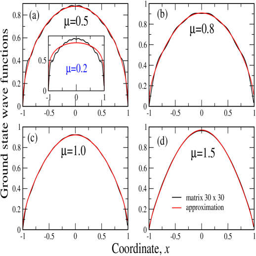
Figure 1: Comparison of ”exact” (for 30x30 matrix diagonalization, see zaba3 ) and approximate (Eqs. (36) - (40)) ground state functions for different stability indices $\mu$ (here our proviso is to use the notation $\mu$ instead of $\alpha$), shown in the panels. The inset to panel (a) reports the case of $\mu=0.2$, when the approximation becomes less accurate than this observed in $\mu\geq 0.5$ regimes, stefthanks .

Remark 1: The $(1-x^{2})^{\alpha/2}$ behavior of the approximate ground state function (35), clearly conforms with results established in the mathematical literature, concerning the near-boundary properties of the involved ”true” eigenfunction $\phi_{1}(x)$ corresponding to the bottom eigenvalue of $(-\Delta)_{D}^{\alpha/2}$ (here, in the interval $[-1,1)$). Namely, it is known that for $x\in D$, we have a two-sided inequality

$$c_{1}\delta^{\alpha/2}(x)\leq\phi_{1}(x)\leq c_{2}\delta^{\alpha/2}(x)$$

where $\delta(x)=dist(x,\partial D)$, while constants $c_{1},c_{2}$ depend on $D$ and the stability index $\alpha$, see e.g. kulczycki ; kulczycki1 . In the interval $(-1.1)$ that amounts to the comparability criterion $\phi_{1}(x)\approx c_{3}\,(1-x^{2})^{\alpha/2}$, where $c_{3}$ is a suitable constant.

Remark 2: The semigroup $T_{t}^{D}(\alpha)=\exp(-t(-\Delta)^{\alpha/2}_{D}$, $t\geq 0$ of the stable process killed upon exiting from a bounded set $D$ has an eigenfunction expansion of the form (7). Basically we never have in hands a complete set of eigenvalues and eigenfunctions and likewise we generically do not know a closed analytic form for the semigroup kernel $k_{D}(t,x,y)$, (7). A genuine mathematical achievement has been to establish that when $\alpha\in(0,2)$ and a bounded domain $D$ is a subset of $R^{n}$, then the stable semigroup $T_{t}^{D}(\alpha)$ is intrinsically ultracontractive. This technical (IU) property actually means that for any $t>0$ there exists $c_{t}$ such that for any $x,y\in D$ we have, kulczycki :

$$k_{D}(t,x,y)\leq c_{t}\,\phi_{1}(x)\phi_{1}(y).$$

Actually we have $k_{D}(t,x,y)=\sum_{1}^{\infty}e^{-\lambda_{n}t}\phi_{n}(x)\phi_{n}(y)$. Accordingly:

$${\frac{k_{D}(t,x,y)}{e^{-\lambda_{1}t}\phi_{1}(x)\phi_{1}(y)}}=1+\sum_{2}^{\infty}e^{-(\lambda_{n}-\lambda_{1})t}\,{\frac{\phi_{n}(x)\phi_{n}(y)}{\phi_{1}(x)\phi_{1}(y)}}.$$

It follows that we have a complete information about the (large time asymptotic) decay of relevant quantities:

$$lim_{t\rightarrow\infty}{\frac{k_{D}(t,x,y)}{e^{-\lambda_{1}t}\phi_{1}(x)\phi_{1}(y)}}=1$$

and (for $t>1$)

$$e^{-(\lambda_{2}-\lambda_{1})t}\leq sup_{x,y\in D}|{\frac{k_{D}(t,,x,y)}{e^{-\lambda_{1}t}\phi_{1}(x)\phi_{1}(y)}}|\leq C_{\alpha,D}e^{-(\lambda_{2}-\lambda_{1})t}.$$

Thus, what we actually need to investigate the large time regime of Lévy processes in the bounded domain $D$, is to know two lowest eigenvalues $\lambda_{1},\lambda_{2}$ and the ground state eigenfunction $\phi_{1}(x)$ of the motion generator.

Remark 3: The existence of conditioned Lévy flights, with a transition density (11) and an invariant probability density $\rho(y)=[\phi_{1}(y)]^{2}$, $\int_{D}\rho(y)\,dy=1$ is here granted as well.

V.3 Spectral Dirichlet case

In the bounded domain, the spectral definition (21) of the Dirichlet fractional Laplacian, effectively reduces to $(-\Delta_{\cal{D}})^{\alpha/2}f(x)=\sum_{j=1}^{\infty}\lambda_{j}^{\alpha/2}f_{j}\phi_{j}(x)$, whose eigenfunctions are shared with the standard Dirichlet Laplacian $(-\Delta_{\cal{D}})$, while the corresponding eigenvalues are raised to the power $\alpha/2$, e.g. read $\lambda_{n}^{\alpha/2}$, $n\geq 1$. we emphasize that the boundary data refer to the boundary $\partial D$ of $D$ only.

In the context of jump-type processes that are killed at the boundary, the spectral definition has been used explicitly in Ref. gitterman , through a direct analog of the transition density (26):

$$k^{\alpha}_{\cal{D}}(t,x,y)={\frac{2}{L}}\sum_{n=1}^{\infty}\sin\left({\frac{n\pi}{L}}(x-a)\right)\sin\left({\frac{n\pi}{L}}(y-a)\right)\exp\left[\left(-{\frac{n\pi}{L}}\right)^{\alpha}t\right].$$ (41)

Here $0<\alpha<2$. All elements of our discussion of asymptotic properties of the corresponding random motion, c.f. Sections II and V remain valid in the present spectral case. In Ref. buldyrev a comparison has been made of the spectral and restricted Dirichlet definitions of fractional Laplacians. Numerical results for various average quantities do not substantially differ. It has been noticed that the restricted Laplacian eigenfunctions are close to the spectral Laplacian eigenfunctions (trigonometric functions) except for the vicinity of the boundaries.

However, in view of the spectral formula (34), the time rate formulas of the form (8),(9), (11), (27) and those listed in Remark 2 show up detectable differences. It is also instructive to make a direct comparison of the pure Brownian case (Section V.A) against the spectral one.

V.4 Regional (censored vs reflected) Lévy flights

Reflected Lévy flights in bounded domains as yet have not received a broad coverage in the literature, bogdan ; reflected and the censored ones likewise. Leaving the mathematical research thread somewhat aside, let us focus on interesting findings in this connection, in the physics-oriented publications, denisov ; dubkov .

Namely, in Ref. denisov steady state (stationary) probability densities for Lévy flights in the interval $[-c,c]$, $L=2c$ (actually for an infinite well) have been derived.

The departure point has been the standard fractional equation of the form (we scale away all dimensional coefficients), c.f. Eq. (9) in Ref. denisov :

$$\partial_{t}f(x,t)=-(-\Delta)^{\alpha/2}f(x,t)$$ (42)

Infinitely deep potential well conditions are set in two steps,

The first one amounts to a demand that $f(x,t)=0$ for all $|x|>c$ while an interval of interest is [-1,1] and we say nothing specific about the values of $f(x,t)$ at the boundary $\partial D$ of $D$. (The boundaries may be impenetrable, but the process make take values on $\partial D$).

For the second step, we invoke the hypersingular integral formula (33), here adapted to the interval $[-c,c]$ instead of the original $[-1,1]$.

The stationarity condition is imposed in the form $\partial_{t}f(x,t)=0$, presuming that the spectrum of the generator (33) contains $0$ as the bottom eigenvalue ((that in view of $(-\Delta)^{\alpha/2}\phi_{n}(x)=\lambda_{n}\phi_{n}$). Hence, we can formally write

$$(-\Delta)^{\alpha/2}f(x)=\int_{-c}^{c}{\frac{f(u)du}{|x-u|^{1+\alpha}}}=0.$$ (43)

The major assumption in Ref. denisov (by no means obvious and potentially questionable in view of hypersingular integral involved) is that Eq. (43) can be represented in the divergence form: $\\ nablaj(x)=0$. It is an auxiliary condition, that the (formally) resulting $j(x)$ vanishes everywhere in $[-c,c]$, from which there follows the $L^{1}[-c,c]$ normalized probability density, denisov , in the closed analytic form:

$$\rho_{\alpha}(x)=(2c)^{1-\alpha}{\frac{\Gamma(\alpha)}{\Gamma^{2}(\alpha/2)}}(c^{2}-x^{2})^{\alpha/2-1},$$ (44)

valid for all $0<\alpha\leq 2$.

The special case of the Cauchy noise ($\alpha=1$) has been addressed in Ref. dubkov , by an independent reasoning, with the outcome:

$$\rho_{1}(x)={\frac{1}{\pi}}{\frac{1}{\sqrt{c^{2}-x^{2}}}}$$ (45)

valid for all $|x|<c$.

In passing we note that for $\alpha=2$ a uniform Brownian distribution $1/L$ arises. That would suggest a link with reflected processes.

At the moment we cannot give an exhaustive analysis of affinities and/or differences between the censored and reflected Lévy processes. As well we do not have a clear understanding whether the process, associated with any probability density $\rho_{\alpha}(x)$ given above, is or is not a reflected stable processes, which take values at $\partial D$.

In the whole stability parameter range $0<\alpha<2$, the probability density $\rho_{\alpha}(x)$, Eq. (44), blows up to infinity at the interval boundaries. Hence, the reflection condition of Ref. reflected for $\alpha=1$ is manifestly violated: $\partial_{x}\rho_{1}(x)=x/\pi(c^{2}-x^{2})^{3/2}$ blows up to $\pm$ infinity at the interval boundaries, instead of vanishing there. This issue needs further analysis.

VI Prospects

We have described comparatively various aspects of random motion (Brownian and Lévy-stable), contributing to the ongoing discussion (both from a a purely mathematical and more pragmatic, basically computer assistance oriented, points of view). Definitely there is some freedom in the definition of Lévy generators in a bounded domain that results in giving access to new, not yet exhaustively investigated, Lévy-type stochastic processes. Their similarities and differences are surely worth an analysis as well. Additionally, some of the pertinent definitions (specifically the spectral one) have gained popularity in the study of nonlinear fractional problems (related to porous media), where they have proved to yield quite efficient computer routines, see e.g. vazquez ; bonforte .

References

- (1) M. Kwaśnicki, ”Ten equivalent definitions of the fractional Laplace operator”, Frac. Calc. Appl. Anal. 20(1), 7–51, (2017).
- (2) R. Servadei and E. Valdinoci, ”On the spectrum of two different fractional operators”, Proc. Roy. Soc. Edinburgh Sect. A, 144, 831-855, (2014).
- (3) N. Abatangelo and E. Valdinoci, ”Getting acquainted with the fractional Laplacian”, arXiv:1710.11567, (2017)
- (4) C. Bucur and E. Valdinoci, ”Nonlocal diffusion and applications”, Lecture Notes of the Unione Matematica Italiana, vol. 20, (Springer-Verlag, Cham, 2016).
- (5) C. Bucur, ”Some observations on the Green function for the ball in the fractional Laplace framework”, Commun. Pur. Appl. Anal., 15, 657, (2016).
- (6) G. Grubb, ”Fractional-order operators, boundary problems, heat equations”, arXiv:1712.01196, (2017)
- (7) G. Grubb, ”Regularity of spectral fractional Dirichlet and Neumann problems”, Math. Nachr., 289 (7), 831-844, (2016).
- (8) T. Kulczycki, ”Eigenvalues and Eigenfunctions for Stable Processes”, chap. 4, pp. 73-86, in: K. Graczyk and A. Stos (Eds.), ”Potential Analysis of Stable Processes and its Extensions”, LNM vol. 1980, Springer-Verlag, Berlin (2009).
- (9) T. Kulczycki, ”Intrinsic ultracontractivity for symmetric stable processes”, Bull. Polish Acad. Sci. 46, 325-334, (1998)
- (10) T. Grzywny, ”Instrinsic contractivity for Lévy processes”, Probability and Math. Statistics, 28(1), 91-106, (2008).
- (11) J. L. Vazquez, ”The mathematical theories of diffusion. Nonlinear and fractional diffusion”, arXiv:1706.08241, (2017)
- (12) M. Bonforte, Y. Sire, and J. L. Vazquez, ”Existence, Uniqueness and Asymptotic behaviour for fractional porous medium equations on bounded domains”, Discrete and Continuous Dynamical Systems, 35 (12), 5725-5767, (2015).
- (13) S.Duo, H. Wang and Y. Zhang, ”A comparative study on nonlocal diffusion operators related to the fractional Laplacian”, arXiv:1711.06916, (2017)
- (14) S. Duo and Y. Zhang, ”Computing the ground and first excited states of the fractional Schröodinger equation in an ininite potential well”, Commun. Comput. Phys., 18, 321-350, (2015).
- (15) M. Żaba and P. Garbaczewski, ”Nonlocally induced (fractional) bound states: Shape analysis in the infinite Cauchy well”, J. Math. Phys. 56, 123502, (2015).
- (16) E. V. Kirichenko, P. Garbaczewski, V. Stephanovich and M. Żaba, ”Ultrarelativistic (Cauchy) spectral problem in the infinite well”, Acta Phys. Pol. B 47(5), 1273-1291, (2016).
- (17) E. V. Kirichenko., P. Garbaczewski, V. Stephanovich and M. Żaba, ”Lévy flights in an infnite well as a hypersingular Fredholm problem”, Phys. Rev. E 93, 052110, (2016).
- (18) K. Bogdan, K. Burdzy and Z. Q. Chen, ”Censored stable processes”, Probab. Theory Relat. Fields 127, 89–152, (2003).
- (19) Q. Y. Guan and Z. M. Ma, ”Reflected symmetric -stable processes and regional fractional Laplacian”, Probab. Theory Relat. Fields 134, 649–694 (2006).
- (20) S. Redner, A Guide to First-passage Processes, (Cambridge University Press, Cambridge 2001).
- (21) M. Gitterman, ”Mean first passage time for anomalous diffusion”, Phys. Rev. E 62, 6065, (2000).
- (22) S. V. Buldyrev et al., ”Average time spent by Lévy flights and walks on an interval with absorbing boundaries”, Phys. Rev. E 64, 041108, (2001).
- (23) B. Dybiec, E. Gudowska-Nowak and P. Hänggi, ”Lévy Brownian motion on finite intervals: Mean first passage time anlysis”, Phys. Rev. E 73, 046104, (2006).
- (24) A. Zoia, A. Rosso and M. Kardar, ”Fractional Laplacian in a bounded domain”, Phys. Rev. E 76, 021116, (2007).
- (25) S. I. Denisov, W. Horsthemke and P. Hänggi, ”Steady-state Lévy flights in a confining domain”, Phys. Rev. E 77, 061112, (2008).
- (26) A. A. Kharcheva et al, ”Spectral characteristics of steady-state Lévy flights in confinement potential profiles”, J. Stat. Mech. vol. 2016 (5),054039; doi:10.1088/1742-5468/2016/05/054039.
- (27) B. Dybiec et al., ”Lévy flights versus Lévy walks in bounded domains”, Phys. Rev. E 95, 052102, (2017).
- (28) P. Garbaczewski, ”Killing (absorption) versus survival in random motion”, Phys. Rev. E 96, 032104, (2017).
- (29) R. G.Pinsky, ”On the convergence of diffusion processes conditioned to remain in a bounded region for large time to limiting positive recurrent processes”, Annals of Probability, 13(2), 363, (1985).
- (30) P. Garbaczewski and M. Żaba, ”Nonlocal random motions and the trapping problem”, Acta Phys. Pol. B 46, 231-246, (2015).
- (31) P. Collet, S. Martinez and J. S. Martin, ”Quasi-Stationary Distributions”, (Springer-Verlag, Berlin, (2013)).
- (32) S. Martinez and J. S. Martin, ”Quasi-stationary distributions for a Brownian motion with drift and associated limit laws”, J. Appl. Prob.31, 911-920, (1994).
- (33) K. Bogdan, Z. Palmowski and L. Wang, ”Yaglom limit for stable processes in cones”, arXiv:1612.03548, (2016).
- (34) A. E. Kyprianou and Z. Palmowski, ”Quasi-stationary distributions for Lévy processes”, Bernoulli, 8(4), 571-581, (2006).
- (35) V. Linetsky, ”On the transition desities for reflected diffusions”, Adv. App. Prob. 37, 435-460, (2005)
- (36) T. Bickel, ”A note on confined diffusion”, Physica A 377, 24-32, (2007).
- (37) P. Garbaczewski and V. Stephanovich, ”Lévy flights and nonlocal quantum dynamics”, J. Math. Phys. 54, 072103, (2013).
- (38) K. Kaleta and J. Lőrinczi, ”Transition in the decay rates of stationary distributions of Lévy motion in an energy landscape”, Phys. Rev. E 93, 022135, (2016).
- (39) M. Kwaśnicki, Eigenvalues of the fractional Laplace operator in the interval, J. Funct. Anal. 262, 2379, (2012).
- (40) T. Kulczycki, M. Kwaśnicki, J. Małecki, and A. Stós, ”Spectral properties of the Cauchy process on half-line and interval”, Proc. London Math. Soc. 101, 589–622, (2010).
- (41) P. Garbaczewski and V. Stephanovich, ”Lévy flights in confinig potentials”, Phys. Rev. E 80, 031113, (2009).
- (42) P. Garbaczewski and V. Stephanovich, ”Lévy flights in inhomogeneous environments”, Physica A 389, 4419, (2010).
- (43) M. Żaba and P. Garbaczewski, ”Solving fractional Schrödinger-type spectral problems : Cauchy oscillator and Cauchy well”, J. Math. Phys. 55, 092103, (2014).
- (44) P. Garbaczewski and M. Żaba, ”Nonlocal random motions and the trapping problem”, Acta Phys. Pol. B 46, 231, (2015)
- (45) M. Żaba and P. Garbaczewski, ”Ultrarelativistic bound states in the spherical well”, J. Math. Phys. 57, 072302, (2016).
- (46) M. Żaba and P. Garbaczewski, ”Ultrarelativistic bound states in the shallow spherical well”, Acta Phys. Pol. B 49(2), (2018).
- (47) J. Lőrinczi and J. Małecki, ”Spectral properties of the massless relativistic harmonic oscillator”, J. Diff. Equations, 253, 2846, (2012)
- (48) J. Lőrinczi, K. Kaleta and S. O. Durugo, ”Spectral and analytic properties of non-local Schródinger operators and related jump processes”, Comm. Appl. and Industrial Math. 6(2), e-534, (2015); DOI: 10.1685/journal.caim.534.
- (49) V. A. Stephanovich, private communication