Dissipative quantum mechanics beyond Bloch-Redfield: A consistent weak-coupling expansion of the ohmic spin boson model at arbitrary bias

Abstract

The ohmic spin boson model at finite bias $\epsilon$ and tunneling $\Delta$ is an important model to study relaxation and decoherence properties of qubits coupled weakly to a dissipative bosonic environment. Fault-tolerant quantum computation requires the investigation of small errors beyond Bloch-Redfield theory. Using perturbation theory and the real-time renormalization group (RG) method we present a consistent zero-temperature weak-coupling expansion for the time evolution of the reduced density matrix $\rho(t)$ out of an uncorrelated but otherwise arbitrary initial state. We show that standard Born approximation schemes calulating the effective Liouvillian of the kinetic equation up to first order in the dimensionless coupling constant $\alpha$ are not sufficient to account for various important corrections one order beyond the Bloch-Redfield solution: (1) The resummation of all secular terms $\sim(\Gamma t)^{n}$ is necessary to obtain the correct exponential decay of all terms of the time evolution with decay rate $\Gamma$ or $\Gamma/2$, together with the correct preexponential functions. We show that this is only possible by a correct analytic continuation of the Fourier transform $L(E)$ of the effective Liouvillian into the lower half of the complex plane. (2) The resummation of all logarithmic terms at high and low energies leads to a renormalized tunneling $\tilde{\Delta}$ and to preexponential functions of logarithmic and power-law form. This is achieved by solving closed differential equations for the derivatives of $L(E)$ set up by the real-time RG method. (3) The fact that two eigenvalues of $L(E)$ are close to each other by $O(\Gamma)$ requires degenerate perturbation theory for times $\Gamma t\sim O(1)$, where certain terms of the Liouvillian in $O(\alpha^{2})$ are needed to calculate the stationary state and the time evolution of the non-oscillating purely decaying terms up to $O(\alpha)$. Solving the real-time RG equations perturbatively we present a renormalized perturbation theory with analytical results for arbitrary bias covering the whole crossover regime from small times $\Omega t\ll 1$ to large times $\Omega t\gg 1$, where $\Omega=\sqrt{\epsilon^{2}+\tilde{\Delta}^{2}}$ denotes the renormalized level splitting, and compare to other results published in the literature. We find that branch cuts starting at pole positions lead to rather slowly varying logarithmic time dependencies for the preexponential functions, whereas pure branch cuts give rise to a strong time dependence of the preexponential functions in the crossover regime with a leading long time tail $\sim\alpha/(\Omega t)$ at finite bias, besides other terms $\sim\alpha/(\Omega t)^{2}$ well-known from the zero-bias case. For exponentially large times, we use the real-time RG method for a non-perturbative resummation of all logarithmic terms $\sim(\alpha\ln(\Omega t))^{n}$ and present a numerical solution for arbitrary bias. We find an interesting power-law behaviour $({1\over\Omega t})^{2\alpha{\epsilon^{2}\over\Omega^{2}}}$ with a bias-dependent power-law exponent appearing in the preexponential functions of the oscillating terms. This power-law has to be contrasted to the one at exponentially small times where the power-law exponent crosses over to $2\alpha$. We discuss that the complexity to calculate one order beyond Bloch-Redfield is rather generic and applies also to other models of dissipative quantum mechanics.

I Introduction

The study of the dynamics of two-state quantum systems coupled weakly to a dissipative bath is a fundamental problem of nonequilibrium statistical mechanics that has become of increasing importance due to possible future technological applications in quantum information processing. To realize scalable and fault-tolerant quantum computation very low error thresholds are needed which requires an understanding beyond Markov approximation schemes and lowest order perturbation theory in the coupling to the bath. As a generic model for a bosonic bath the spin-boson model has been proposed leggett_87 and its dynamical properties have been studied with various methods weiss_12 ; grifoni_haenggi_98 . This model consists of two levels with level spacing (bias) $\epsilon$, coupled by a direct tunneling term $\Delta$, and each level is linearly coupled to an ohmic bosonic bath. In the case of zero tunneling, the spin-boson model can be solved exactly and the stability of surface-code error correction against realistic dissipation has been studied recently hutter_loss_13 ; novais_mucciolo_13 . However, for finite tunneling and the most important case of an ohmic coupling to the bath, we will show in this work that a consistent weak-coupling expansion beyond the Bloch-Redfield Markov approximation is still lacking at low temperatures. We will discuss various subtleties to obtain a consistent perturbative expansion of the time evolution in the dimensionless coupling constant $\alpha$, requiring an essentially non-perturbative treatment in a certain sense, not yet accounted for completely in various previous publications on the ohmic spin boson model. Most importantly, our analysis shows that the systematic calculation of errors to the Bloch-Redfield result is generically very complex for all models of dissipative quantum mechanics, involving many details of the underlying model, and is not specific to the ohmic spin boson model.

The concrete form of the time evolution depends crucially on the form of the density of states of the bath and the energy dependence of the coupling constants $g_{q}$ of the local system to the various bath modes $\omega_{q}$, conveniently taken together in the spectral density (sometimes also called hybridization function) $J(\omega)\sim\sum_{q}g_{q}^{2}\delta(\omega-\omega_{q})$. However, for a flat spectral density (on the scale of the typical energy scales of the local system) or for special cases as the ohmic spin boson model, where $J(\omega)\sim\alpha\omega$, a rather generic discussion of the typical form of the time evolution is possible and has been provided in Ref. pletyukhov_schuricht_schoeller_10, , based on the real-time renormalization group method (RTRG), see Rfs. schoeller_09, ; schoeller_14, for reviews. Starting at time $t=0$ from an arbitrary initial state $\rho_{0}=\rho(t=0)$ of the local system without any initial system-bath correlations (i.e. the bath is assumed to be an infinitely large system in (grand)canonical equilibrium), the time evolution for the reduced density matrix $\rho(t)$ of the local system consists of a sum of terms each of them being $\sim{\cal{F}}_{i}(t)e^{-iz_{i}t}$, with $z_{i}=\Omega_{i}-i\Gamma_{i}$, i.e. exponentially decaying with decay rate $\Gamma_{i}>0$, oscillating with frequency $\Omega_{i}$, together with a non-exponential preexponential function ${\cal{F}}_{i}(t)$, typically depending logarithmically or as some power-law on time. The case $\Gamma_{i}=0$ is exceptional and occurs only for systems with quantum critical points, where the scaling behavior is not cut off by any decay rate. For the ohmic spin boson model there are three modes of a purely decaying mode $z_{0}=-i\Gamma$ and two oscillating modes with $z_{\pm}=\pm\Omega-i\Gamma/2$. This form already suggests where the complexity of calculating the time evolution beyond the lowest order Markovian Bloch-Redfield theory appears. Bloch-Redfield considers only the leading order term where ${\cal{F}}_{i}$ is basically a constant of $O(1)$, independent of the coupling $\alpha$ to the bath. However, there are additional terms to each matrix element of the $2\times 2$-matrix $\rho(t)$, where ${\cal{F}}_{i}(t)\sim\alpha$, also containing an exponential function, usually different from the one of the Bloch-Redfield term. Expanding this exponential in $\Gamma\sim\alpha$ leads to an ill-defined perturbation expansion, since terms $\sim\alpha(\Gamma t)^{n}$ appear, which all become of $O(\alpha)$ already on time scales of the inverse decay rate (and even diverge for time going to infinity). Therefore, for a consistent calculation of the $O(\alpha)$ correction to Bloch-Redfield on time scales where the exponential damping is still moderate, it is necessary to resum these terms in all orders of perturbation theory to get the correct exponential behavior. We note that these so-called secular terms (sometimes also called van Hove singularities van_hove_loss ) are usually only discussed when expanding the exponentials of the Bloch-Redfield terms in $\alpha$, but similarly also appear in higher order terms, which are more subtle. Technically, they can all be incorporated by expressing the perturbative expansion for the effective Liouvillian $L(E)$ in Fourier space not in terms of the bare Liouvillian but in terms of the full Liouvillian again by taking all self-energy insertions into account. Within the diagrammatic expansion developed in Rfs. schoeller_09, ; schoeller_14, ; pletyukhov_schoeller_12, ; kashuba_schoeller_13, it can be seen that this is possible in all orders of perturbation theory. This allows for a convenient analytic continuation of $L(E)$ into the lower half of the complex plane, from which the position of all non-zero singularities $z_{i}$ (poles and branching points) of the Fourier transform $\rho(E)=i/(E-L(E))\rho_{0}$ can be determined self-consistently, leading to the effect that all $z_{i}$ acquire a finite imaginary part $-i\Gamma_{i}$.

In connection with the ohmic spin boson model at zero bias, the occurrence of exponentials in the $O(\alpha)$-correction to Bloch-Redfield has recently been noted and corrected in Rfs. slutskin_etal_11, ; kashuba_schoeller_13, . Similar considerations have been performed close to $\alpha\sim{1\over 2}$, see Rfs. egger_etal_97, ; kennes_etal_13, . For finite bias, a Born approximation has been used in Ref. divincenzo_loss_05, to calculate perturbatively one order beyond Bloch Redfield, missing the exponentials in those corrections. In this paper we will present a perturbative calculation at arbitrary bias including all exponentials and, moreover, show that the resummation of secular terms is also important to obtain the correct energy scales in logarithmic terms of preexponential functions. Furthermore, we will calculate all terms of the time evolution for an arbitrary initial state of the local system, whereas in Ref. divincenzo_loss_05, only the time evolution of the Pauli matrix in $z$-direction has been calculated for an initial state without any spin in $x-$ and $y-$ direction.

Besides secular terms proportional to powers of time, there are further subtleties in the calculation of the time evolution, even in the case where potential logarithmic terms can be treated perturbatively. A generic feature of the reduced density matrix $\rho(E)=i/(E-L(E))\rho_{0}$ in Fourier space is that there occurs one singularity at $E=0$ (determining the stationary state from $L(0^{+})\rho_{\text{st}}=0$) and a pure decay pole at $E=z_{0}=-i\Gamma\sim O(\alpha)$. These two singularities are close to each other within the expansion parameter $\alpha$, and leads to the generic feature that two eigenvalues of $L(E)$ are close to each other by $O(\alpha)$. Therefore, degenerate perturbation theory is necessary for the zero and purely decaying modes, and the calculation of the corresponding projectors on the eigenstates of $L(E)$ up to $O(\alpha)$ requires the knowledge of the Liouvillian at least up to $O(\alpha^{2})$. This fact has already been mentioned at the end of Ref. divincenzo_loss_05, , where the stationary state was calculated up to $O(\alpha)$ and the influence on the time evolution for the purely decaying mode was indicated. This again is a generic problem for all models of dissipative quantum mechanics and shows that lowest order Born approximation is not sufficient to account for all first-order corrections to Bloch-Redfield. In this paper we will show that the special algebra of the ohmic spin model allows for a simplification of this problem such that the results of Ref. divincenzo_loss_05, for the stationary case up to $O(\alpha)$ can be used to calculate also all terms in $O(\alpha)$ for the time evolution of the purely decaying mode.

The ohmic spin boson model (and similar many other models with a rather structureless spectral density of states) has further problems in perturbation theory arising from logarithmically divergent integrals at high and low energies, which have to be treated by renormalization group. At high energies logarithmic divergencies $\sim\alpha\ln{D/\Lambda_{c}}$ occur, where $D$ denotes the finite band width and $\Lambda_{c}\sim\text{max}\{1/t,\Omega\}$ is some high-energy cutoff determined by the largest energy scale of the system. For large $D$ a non-perturbative resummation of all powers of such terms is required. In the short-time regime $1/t\gg\Omega$, this leads to well-known terms $\sim 1/(Dt)^{2\alpha}$ which can also be obtained from the noninteracting blip approximation (NIBA) leggett_87 ; weiss_12 . For the most important regime of times which are not exponentially small or large, where $|\alpha\ln(\Omega t)|\ll 1$, we will show in this paper that the logarithmic terms at high energies can be incorporated into a renormalized tunneling $\tilde{\Delta}=\Delta(\Omega/D)^{\alpha}$, where $\Omega=\sqrt{\epsilon^{2}+\tilde{\Delta}^{2}}$ is the renormalized Rabi frequency of the local system, leading also to a renormalized decay rate $\Gamma=\pi\alpha\tilde{\Delta}^{2}/\Omega$. We note that the correct cutoff scale is $\Lambda_{c}=\Omega$ and not $\tilde{\Delta}$ as first pointed out in Ref. divincenzo_loss_05, , where the logarithmic correction was calculated perturbatively in $\alpha$. Furthermore, we will show in this paper how the unrenormalized tunneling occurring in various terms of perturbation theory has to be replaced by the renormalized one. This is quite nontrivial since both $\Delta$ and $\tilde{\Delta}$ appear in the final solution. We will achieve this goal by solving the RTRG equations perturbatively with the result of a renormalized propagator containing $Z$-factors with $Z=\tilde{\Delta}^{2}/\Delta^{2}$. Subsequently, we will apply renormalized perturbation theory to calculate the time evolution analytically in the whole crossover regime from small times $\Omega t~{}\ll 1$ to large times $\Omega t\gg 1$ with $|\alpha\ln(\Omega t)|\ll 1$ such that logarithmic terms in time can be treated perturbatively. We find that the leading order terms in the preexponential functions stem from branch cuts starting at a pole position of $\rho(E)$ giving rise to constant terms together with terms $\sim\alpha\ln(\Omega t)$ showing a rather weak logarithmic time dependence. In contrast, branch cuts starting at branching points unequal to the poles of $\rho(E)$ lead to crossover functions with a strong time dependence of the preexponential functions which all can be expressed by the exponential integral. Interestingly, for large times $\Omega t\gg 1$, we find that the leading order terms fall off $\sim\alpha/(\Omega t)$ for finite bias, in contrast to the unbiased case, where all terms fall off $\sim\alpha/(\Omega t)^{2}$.

After having got rid of logarithmic terms at high energies, one is still left with logarithmic terms at low energies $\sim\alpha\ln{\Omega t}$. If the latter can be treated perturbatively, the solution for the time evolution one order beyond Bloch-Redfield follows from the above mentioned renormalized perturbation theory with the proper replacement of $\Delta$ by $\tilde{\Delta}$. However, for intermediate couplings $\alpha\sim 0.1-0.2$ or for the case of high bias $\epsilon\gg\tilde{\Delta}$ (where the decay rate $\Gamma\ll\alpha\Omega$ is very small), it turns out that higher order terms $\sim(\alpha\ln{\Omega t})^{n}$ with $n>1$ become important already for times scales $t\sim 1/\Gamma$. In these cases a non-perturbative resummation is also necessary for the logarithmic terms at low energies to determine the first correction to Bloch-Redfield consistently. The only available method up to date to achieve such a resummation is the RTRG method schoeller_09 ; schoeller_14 ; pletyukhov_schoeller_12 ; kashuba_schoeller_13 , which can account simultaneously for logarithmic terms at high and low energies in all orders to determine the time evolution of models of dissipative quantum mechanics in the weak coupling regime. The idea is not to consider the perturbative expansion of the effective Liouvillian $L(E)$ but of the second derivative ${\text{d}^{2}\over\text{d}E^{2}}L(E)$, together with a proper resummation of self-energy insertions and vertex corrections. This leads to a set of closed differential equations for the effective Liouvillian and the effective vertices, which are well-defined in the limit $D\rightarrow\infty$ and contain no secular terms and logarithmic divergencies at low and high energies. Therefore, the r.h.s. of these differential equations are a well-defined series in $\alpha$ and can be truncated systematically. We will consider the RG equations in leading order and solve them numerically for the ohmic spin boson model at arbitrary bias. Most importantly, we find for the leading order terms of the preexponential functions of the oscillating modes a power-law behaviour $\sim 1/(\Omega t)^{2\alpha{\epsilon^{2}\over\Omega^{2}}}$ for exponentially large times, where the power-law exponent interpolates between $1$ for $\epsilon=0$ and $2\alpha$ for $\epsilon\gg\tilde{\Delta}$. The bias-dependent power-law exponent $2\alpha{\epsilon^{2}\over\Omega^{2}}$ has also been proposed in Ref. slutskin_etal_11, but we stress that it is only correct for very large times and we will show that, for small times, other logarithmic contributions appear which lead to a complicated crossover to a power-law $\sim 1/(\Omega t)^{2\alpha}$ for exponentially small times. As already mentioned in Ref. kashuba_schoeller_13, , the determination of the correct long-time behavior of preexponential functions depends crucially on the vertex renormalization not taken into account in any previous work. At zero bias this has lead to a correction of the NIBA-result kashuba_schoeller_13 and we stress that all our results for nonzero bias presented in this paper can as well only be derived correctly by including the vertex renormalization.

The paper is organized as follows. In Section II we introduce the ohmic spin boson model and the kinetic equation to calculate the time dynamics. We provide the perturbative expansion of the effective Liouvillian in Fourier space and explain its analytic structure together with the one of the reduced density matrix. We also provide the propagator in renormalized perturbation theory which will be derived later in Section IV. In Section III we will explicitly calculate the time dynamics in various time regimes. We review the exact solution at zero tunneling and the Bloch-Redfield solution in Sections III.1 and III.2 as a reference. In Section III.3 we present the results from renormalized perturbation theory and determine the time evolution in the regime of small times in Section III.3.1 and in the whole regime where time is not exponentially small or large in Section III.3.2. In Section IV we use the RTRG method to account for all logarithmic terms nonperturbatively. In Section IV.1 we set up the RG equations for the ohmic spin boson model and show in Sections IV.2 and IV.3 how the propagator has to be changed to account for all logarithmic renormalizations from high energies. The numerical solution of the RG equations containing also all logarithmic renormalizations at low energies will be presented in Section IV.4. We close with a summary of our results in Section V and discuss their relevance for other models of dissipative quantum mechanics. We use the unit $\hbar=1$ throughout this paper.

II Model, kinetic equation and Liouvillian

In this Section we introduce the model under consideration and set up the kinetic equation to determine the time dynamics of the local reduced density matrix. In addition we provide the perturbative solution for the effective Liouvillian in Fourier space. This form is very helpful to understand the proper analytical continuation into the lower half of the complex plane and the correct procedure to avoid the occurrence of secular terms. Furthermore, we will present the perturbative determination of the decay poles.

II.1 Model

The Hamiltonian for the spin boson model consists of a local $2$-level system (described by Pauli matrices $\sigma_{i}$) coupled linearly to a bosonic bath with energy modes $\omega_{q}>0$

$$H_{\text{tot}}\, =\,H\,+\,H_{\text{bath}}\,+\,V\quad,$$ (1)

$$H\, =\,{\epsilon\over 2}\sigma_{z}\,-\,{\Delta\over 2}\sigma_{x}\quad,$$ (2)

$$H_{\text{bath}}\, =\,\sum_{q}\omega_{q}a_{q}^{\dagger}a_{q}\quad,$$ (3)

$$V\, =\,{1\over 2}\sigma_{z}\,\sum_{q}g_{q}(a_{q}+a_{q}^{\dagger})\quad,$$ (4)

where $\epsilon$ denotes the bias, $\Delta$ the tunneling, and the coupling to the bath is described by the coupling parameters $g_{q}$. We note that by a convenient spin rotation the coupling to the bath can always be chosen in the z-direction and the y-axis can be chosen perpendicular to the local spin in the Hamiltonian (the expectation value of the local spin will of course get all components as function of time). The parameters $\epsilon$, $\Delta$ and $g_{q}$ are real to guarantee hermiticity of $H_{\text{tot}}$ (please note that the sign convention for $\Delta$ is sometimes chosen differently in the literature). For convenience we choose $\Delta,\epsilon>0$ which again can always be achieved by an appropriate spin rotation.

The microscopic details of the modes $\omega_{q}$ and the coupling constants $g_{q}$ enter the time dynamics of the local system only via the energy dependence of the spectral density

$$J(\omega)\,=\,\pi\sum_{q}g_{q}^{2}\delta(\omega-\omega_{q})\quad,$$ (5)

which, for the ohmic spin boson model, is parametrized as

$$J(\omega)\,=\,2\pi\alpha\omega\theta(\omega)J_{c}(\omega)\quad,$$ (6)

where $\alpha$ is a dimensionless coupling constant and $J_{c}(\omega)$ is a high-energy cutoff function needed since frequency integrals diverge logarithmically at high energies for all terms in the perturbative series in $\alpha$. In this paper we choose a Lorentzian cutoff function (in contrast to exponential cutoffs $\sim e^{-\omega/D}$ often used in the literature)

$$J_{c}(\omega)\,=\,{D^{2}\over D^{2}+\omega^{2}}\quad,$$ (7)

where $D$ denotes the band width. This choice is taken to simplify frequency integrals and influences only some prefactors of non-logarithmic terms but not the scaling behavior. The ohmic spin boson model in weak coupling is defined by the condition $\alpha\ll 1$ such that a perturbative expansion in $\alpha$ makes sense.

Since we will also work in a basis where the local Hamiltonian $H$ is diagonal we introduce the unitary transformation

$$U\,=\,U^{\dagger}\,=\,U^{-1}\,=\,{1\over\sqrt{2\Omega_{0}}}\left(\begin{array}[]{cc}-v_{-}&v_{+}\\ v_{+}&v_{-}\end{array}\right)\quad,$$ (10)

where $v_{\pm}=\sqrt{\Omega_{0}\mp\epsilon}$ and

$$\Omega_{0}\,=\,\sqrt{\epsilon^{2}+\Delta^{2}}$$ (11)

denotes the bare level splitting (Rabi frequency) of the local system. With this unitary transformation we get $UHU^{\dagger}={1\over 2}\Omega_{0}\sigma_{z}$, i.e. the eigenvalues $\pm\Omega_{0}/2$ with corresponding eigenvectors given by the two columns of $U^{\dagger}=U$.

II.2 Kinetic equation

We aim at calculating the time dynamics of the reduced density matrix of the local system

$$\rho(t)\,=\,Tr_{\text{bath}}\rho_{\text{tot}}(t)$$ (12)

with an initial state for the total density matrix

$$\rho_{\text{tot}}(t=0)\,=\,\rho_{0}\rho_{\text{bath}}^{\text{eq}}$$ (13)

factorizing into an arbitrary initial state $\rho_{0}=\rho(t=0)$ for the local system and an equilibrium canonical distribution $\rho_{\text{bath}}$ for the bath. For simplicity we set temperature $T=0$ in the following. Using standard projection operator projection_operator , path integral weiss_12 , or diagrammatic schoeller_09 ; schoeller_14 techniques one can show that $\rho(t)$ can be determined from a formally exact kinetic equation

$$i\dot{\rho}(t)\,=\,L_{0}\rho(t)+\int_{0}^{t}dt^{\prime}\Sigma(t-t^{\prime})\rho(t^{\prime})\quad,$$ (14)

where $L_{0}=[H,\cdot]$ and $\Sigma(t-t^{\prime})$ are superoperators acting on operators. The first term on the r.h.s. describes the time evolution from the von Neumann equation of the isolated local system, whereas the second term contains the dissipative kernel $\Sigma(t-t^{\prime})$ leading to irreversible time dynamics into a stationary state $\rho_{\text{st}}=\lim_{t\rightarrow\infty}\rho(t)$. The various methods described in Rfs. projection_operator, ; weiss_12, ; schoeller_09, ; schoeller_14, just differ in the technique how to calculate this kernel in perturbation theory in $\alpha$. Since all quantities are only defined for positive times, we define the Fourier transform as for retarded correlation functions (for convenience we use the same symbol for the Fourier transform)

$$\rho(E)\,=\,\int_{0}^{\infty}dt\,e^{iEt}\rho(t)\quad,\quad\Sigma(E)\,=\,\int_{0}^{\infty}dt\,e^{iEt}\Sigma(t)\quad,$$ (15)

which are well-defined analytic functions in the complex plane for all $E$ with positive imaginary part (a proper analytic continuation into the lower half of the complex plane will be discussed later). From (14) we obtain the formal solution in Fourier space as

$$\rho(E)\,=\,{i\over E-L(E)}\rho_{0}\quad,$$ (16)

where $L(E)=L_{0}+\Sigma(E)$ denotes the effective Liouvillian in Fourier space with matrix elements $L_{s_{1}s_{2},s_{1}^{\prime}s_{2}^{\prime}}$ ($s$ denote the states of the local system). The Liouvillian has the two important properties schoeller_09 ; schoeller_14

$$\text{Tr}L(E)\cdot\,=\,0\quad,\quad L(E)^{c}\,=\,-L(-E^{*})\quad,$$ (17)

where Tr denotes the trace over the local system and the $c$-transform is defined by $L(E)^{c}_{s_{1}s_{2},s_{1}^{\prime}s_{2}^{\prime}}=L(E)_{s_{2}s_{1},s_{2}^{\prime}s_{1}^{\prime}}^{*}$. From these properties one can show the conservation of probability $Tr\dot{\rho}(t)=0$ and the hermiticity of the density matrix $\rho(t)^{\dagger}=\rho(t)$ schoeller_09 ; schoeller_14 .

Once $L(E)$ is known, the time dynamics can be calculated from inverse Fourier transform as

$$\rho(t)\,=\,{i\over 2\pi}\int_{\cal{C}}dE{e^{-iEt}\over E-L(E)}\rho_{0}\quad,$$ (18)

where $\cal{C}$ is a straight line in the complex plane lying slightly above the real axis, i.e. $E=x+i\eta$, with $\eta=0^{+}$ and $x$ running from $x=-\infty$ to $x=+\infty$ (the precise form of $\cal{C}$ in the upper half is not important since $\rho(E)$ is an analytic function there). We note that we have used the Fourier and not the Laplace transform (defined by $e^{-Et}$ in (15)) since it makes the analogy to the analytic properties of retarded correlation functions more transparent.

As pointed out in detail in Rfs. pletyukhov_schuricht_schoeller_10, ; schoeller_09, ; schoeller_14, ; kashuba_schoeller_13, the most elegant way to determine the integral over $\cal{C}$ is to close the integration contour in the lower half of the complex plane and to use a convenient analytic continuation of $L(E)$ and $\rho(E)$ into the lower half of the complex plane, such that all branch cuts point into the direction of the negative imaginary axis and start at the branching points $z_{i}=\Omega_{i}-i\Gamma_{i}$. For the ohmic spin boson model we note that $\rho(E)$ has one isolated pole at $E=0$ determining the stationary state from

$$L(0^{+})\rho_{\text{st}}\,=\,0\quad,$$ (19)

together with three branch cuts starting at the branching points (or poles)

$$z_{0}\,=\,-i\Gamma\quad,\quad z_{\pm}=\pm\Omega-i\Gamma/2\quad,$$ (20)

with $\Gamma>0$, whereas $L(E)$ has only branch cuts starting at $z_{0}$ and $z_{\pm}$ without any poles. If we denote the eigenvalues of the $4\times 4$-matrix $L(E)$ by $\gamma_{i}(E)$ with $i=\text{st},0,\pm$, the pole positions of the propagator $1/(E-L(E))$ follow from $\gamma_{i}(z_{i})=z_{i}$ and it follows from (17) that one eigenvalue must be zero and $-\gamma_{i}(E)^{*}$ are the eigenvalues of $L(-E^{*})$. Thus, $-\gamma_{i}(-E^{*})^{*}$ must be also an eigenvalue of $L(E)$, leading to

$$\gamma_{\text{st}}\, =\,0\quad,$$ (21)

$$\gamma_{0}(E)\, =\,-\gamma_{0}(-E^{*})^{*}\quad,$$ (22)

$$\gamma_{+}(E)\, =\,-\gamma_{-}(-E^{*})^{*}\quad.$$ (23)

As a consequence, the pole $z_{0}$ is purely imaginary and $z_{+}=-z_{-}^{*}$, in accordance with (20).

Using the diagrammatic technique of Rfs. schoeller_09, ; schoeller_14, ; pletyukhov_schoeller_12, ; kashuba_schoeller_13, one can derive the analytic features in all orders of perturbation theory but it is illustrative to study them already from the perturbative solution for $L(E)$ up to $O(\alpha)$, which will be presented in the next Section.

II.3 Liouvillian in perturbation theory

With the help of the diagrammatic technique used in Ref. kashuba_schoeller_13, for the ohmic spin model at zero bias, we calculate the Liouvillian up to $O(\alpha)$ in Appendix A. Denoting the two states of the local system by $i=1,2$ (corresponding to the original Hamiltonian $H$ in (2)) and using the sequence $(11,22,12,21)$ to numerate the matrix elements of superoperators, we find:

$$L(E)\, =\,L_{0}+\Sigma_{a}(E)+\Sigma_{s}=L_{a}(E)+\Sigma_{s}\quad,$$ (24)

$$L_{0}\, =\,\left(\begin{array}[]{cc}0&\Delta\tau_{-}\\ \Delta\tau_{-}&\epsilon\sigma_{z}\end{array}\right)\quad,$$ (27)

$$\Sigma_{s}\, =\,i\pi\alpha\Delta\left(\begin{array}[]{cc}0&0\\ \tau_{+}&0\end{array}\right)\quad,$$ (30)

$$\Sigma_{a}(E)\, =\,\alpha\sum_{i=0,\pm}{\cal{F}}_{i}(E)M_{i}\,\,,\,\,M_{i}=\left(\begin{array}[]{cc}0&0\\ 0&\hat{M}_{i}\end{array}\right)\quad,$$ (33)

$$\hat{M}_{0}\, =\,2{\Delta^{2}\over\Omega_{0}^{2}}\tau_{-}\quad,$$ (34)

$$\hat{M}_{\pm}\, =\,\tau_{+}\,\pm\,{\epsilon\over\Omega_{0}}\sigma_{z}\,+\,{\epsilon^{2}\over\Omega_{0}^{2}}\tau_{-}\quad,$$ (35)

where $\tau_{\pm}={1\over 2}(1\pm\sigma_{x})$ and

$${\cal{F}}_{i}(E)\, =\,(E-\lambda_{i}(E)){\cal{L}}_{i}(E)\quad,$$ (36)

$${\cal{L}}_{i}(E)\, =\,\ln{-i(E-\lambda_{i}(E))\over D}\quad.$$ (37)

Here $\lambda_{i}(E)$ are the important functions

$$\lambda_{0}(E)\, =\,-\alpha{\Delta^{2}\over\Omega_{0}}\sum_{\sigma=\pm}\sigma{\cal{L}}_{\sigma}(E)\quad,$$ (38)

$$\lambda_{\pm}(E)\, =\,\pm(\Omega_{0}+\alpha{\Delta^{2}\over\Omega_{0}}{\cal{L}}_{0}(E))\quad,$$ (39)

which determine the position of the poles (20) of the resolvent $1/(E-L(E))$ (and also of $\rho(E)$ due to (16)) by solving the self-consistent equations

$$z_{i}\,=\,\lambda_{i}(z_{i})\quad.$$ (40)

This can be seen from the derivation in Appendix A, where the $\lambda_{i}(E)$ are defined as the eigenvalues of the Liouvillian $\tilde{L}_{\Delta}(E)$, defined by

$$\tilde{L}_{\Delta}(E)\,=\,Z^{\prime}(E)L_{\Delta}(E)\quad,\quad Z^{\prime}(E)\,=\,{1\over 1-L^{\prime}(E)}\quad,$$ (41)

where $L_{\Delta}(E)$ and $L^{\prime}(E)$ follow from the decomposition

$$L_{a}(E)\, =\,L_{\Delta}(E)\,+\,EL^{\prime}(E)$$

$$=\,L_{0}\,+\,\Sigma_{\Delta}(E)\,+\,EL^{\prime}(E)\quad,$$ (42)

with

$$\Sigma_{\Delta}(E)\, =\,-\alpha\sum_{i=0,\pm}\lambda_{i}(E){\cal{L}}_{i}(E)M_{i}\quad,$$ (43)

$$L^{\prime}(E)\, =\,\alpha\sum_{i=0,\pm}{\cal{L}}_{i}(E)M_{i}\quad.$$ (44)

This decomposition is very helpful since it exhibits the purely logarithmic superoperators $L_{\Delta}(E)$ and $L^{\prime}(E)$, together with the terms linear in $E$. The eigenvalues of $L(E)$ and $\tilde{L}_{\Delta}(E)$ are different but the relation (note that $\Sigma_{s}L_{a}=0$)

$${1\over E-L(E)}\, =\,{1\over E-L_{a}(E)}(1+\Sigma_{s}{1\over E})$$

$$=\,{1\over E-\tilde{L}_{\Delta}(E)}Z^{\prime}(E)(1+\Sigma_{s}{1\over E})\quad,$$ (45)

shows that the poles of the two resolvents $1/(E-L(E))$ and $1/(E-\tilde{L}_{\Delta}(E))$ are the same, i.e. the solutions $z_{i}$ of the self-consistent equations (40) provide indeed the nonzero poles of the resolvent $1/(E-L(E))$.

Most importantly, we see from the perturbative result (24)-(33) that $z_{i}$ are not only the poles of the local density matrix in Fourier space but at the same time determine the branching points of the logarithmic functions ${\cal{L}}_{i}(E)$, i.e. determine the starting points for the branch cuts of $L(E)$ in the lower half of the complex plane. The logarithm in Eq. (37) is the natural logarithm with a branch cut on the negative real axis, i.e. the branch cut w.r.t. the Fourier variable $E$ points into the direction of the negative imaginary axis, a choice which will be most convenient for an analytical determination of the branch cut integral in the long time limit, see Section III. The fact that the branching points of all logarithmic terms are the same as the pole positions of the local density matrix is a very important observation and can be shown to hold in all orders of perturbation theory by using the diagrammatic method developed in Rfs. pletyukhov_schuricht_schoeller_10, ; schoeller_09, ; schoeller_14, ; kashuba_schoeller_13, , see also some remarks in Appendix A. Obviously, for this property it is very important to keep the functions $\lambda_{i}(E)$ in the argument of the logarithm and not to expand ${\cal{L}}_{i}(E)$ in $\alpha$. As already mentioned in Ref. schoeller_14, in all detail, such an expansion leads to secular terms $(1/E)^{n}$ for the Liouvillian, e.g. for the expansion of $\alpha{\cal{F}}_{0}(E)$ one obtains

$$\alpha{\cal{F}}_{0}(E)\, =\,\alpha(E-\lambda_{0}(E))\ln{-iE\over D}-\alpha\lambda_{0}(E)$$

$$+{1\over 2}\alpha\lambda_{0}(E)^{2}{1\over E}+O(\alpha^{4})\quad.$$ (46)

We note that secular terms start at $O(\alpha^{3})$ due to the factor $E-\lambda_{0}(E)$ in front of the logarithm. Therefore, even in a calculation up to $O(\alpha^{2})$ one can not see the occurrence of secular terms in $L(E)$. The power of these secular terms increases with increasing order in $\alpha$ and, therefore, have to be resummed nonperturbatively. They appear directly in the effective Liouvillian $L(E)$ and have to be distinguished from secular terms appearing by expanding the resolvent $1/(E-L_{0}-\Sigma(E))$ in $\Sigma(E)$. The resummation of the latter are responsible to obtain the correct exponential behavior of the leading order Bloch-Redfield terms for the time evolution, whereas the ones in $L(E)$ have to be resummed to obtain the exponential part of all correction terms to the Bloch-Redfield solution. Essentially, the fact that logarithmic functions in all orders of perturbation theory appear always in the form of ${\cal{L}}_{i}(E)$ is due to the property that all bare propagators of the local system can be replaced by full propagators without any double counting, see Appendix A. As a consequence the exact eigenvalues of $\tilde{L}_{\Delta}(E)$ appear in the perturbative series and not the bare ones. This fact is very important to notice in order to find the correct nonanalytic features in the lower half of the complex plane. E.g. by calculating ${\cal{F}}_{0}(E)$ only by the first term on the r.h.s. of (46) one obtains a logarithm which has a branch cut starting at the origin leading to a term of the time evolution which is not exponentially decaying. The expansion (46) is only well-defined for $E\sim\Omega_{0}$, i.e. on time scales $t\sim 1/E\sim 1/\Omega_{0}$, where the solution is just oscillating and the decay has not yet set in. In this regime the perturbative solution of Ref. divincenzo_loss_05, can be used but not for larger time scales describing the crossover to the regime of exponential decay.

We note that the perturbative solution (24)-(33) for $L(E)$ can only be used when the logarithmic terms are small enough, i.e. the condition

$$\alpha|\ln{-i(E-\lambda_{i}(E))\over D}|\,\ll\,1$$ (47)

should hold. This is obviously not fulfilled when $E$ approaches the branching point $z_{i}$ or is too far away from it. Only the RG method presented in Section IV is capable of resumming the logarithmic terms in all orders to find the correct scaling behavior for large $E$ or $E$ close to $z_{i}$. The condition (47) can be reformulated in terms of time by replacing $E-\lambda_{i}(E)\rightarrow 1/t$ leading to

$$\alpha|\ln(Dt)|\,\ll\,1\quad,$$ (48)

showing that the perturbative theory can not be used to calculate the time evolution for exponentially small or large times. However, as we will see in Section IV these regimes can be studied as well by using the RTRG method.

As a consequence one should also not be concerned by the fact that the solution of the self-consistent equations (40) with (38) and (39) is ill-defined due to the singularity of the logarithm. For times in the regime (48) we need the functions $\lambda_{i}(E)$ only in the typical regime (47). Using $z_{0}\sim O(\alpha)$ and $z_{\pm}=\pm\Omega_{0}+O(\alpha)$, this means that for $|E-z_{0}|\sim\alpha^{n}\Omega_{0}$ (with some integer $n>0$) we can replace $\lambda_{0}(E)$ by

$$\lambda_{0}(E)\,\approx\,-\alpha{\Delta^{2}\over\Omega_{0}}\sum_{\sigma=\pm}\sigma\ln{-i(-\sigma\Omega_{0})\over D}\,=\,-i\Gamma_{1}\quad,$$ (49)

with

$$\Gamma_{1}\,=\,\pi\alpha{\Delta^{2}\over\Omega_{0}}\quad,$$ (50)

up to an error of $O(n\alpha^{2}\ln{\alpha})$. Up to the same error, for $|E-z_{\pm}|\sim\alpha^{n}\Omega_{0}$, we can replace $\lambda_{\pm}(E)$ by

$$\lambda_{\pm}(E)\,\approx\,\pm(\Omega_{0}+\alpha{\Delta^{2}\over\Omega_{0}}\ln{-i(\pm\Omega_{0})\over D})\,=\,\pm\Omega_{1}-i\Gamma_{1}/2\quad,$$ (51)

with

$$\Omega_{1}\,=\,\Omega_{0}-\alpha{\Delta^{2}\over\Omega_{0}}\ln{D\over\Omega_{0}}\quad.$$ (52)

Therefore, we conclude from the perturbative expansion that the solution of (40) is given by

$$z^{(1)}_{0}\, =\,-i\Gamma_{1}+O(\alpha^{2}\ln\alpha)\quad,$$ (53)

$$z^{(1)}_{\pm}\, =\,\pm\Omega_{1}-i\Gamma_{1}/2+O(\alpha^{2}\ln\alpha)\quad.$$ (54)

In Section IV we will resum all logarithmic renormalizations $\sim(\alpha\ln(\Omega/D))^{n}$ from high energies and show that $\Omega_{1}$ has to be replaced by the renormalized Rabi frequency $\Omega$, which has the same form as $\Omega_{0}$ but the bare tunneling $\Delta$ has to be replaced by the renormalized tunneling $\tilde{\Delta}$

$$\Omega\, =\,\sqrt{\epsilon^{2}+\tilde{\Delta}^{2}}\quad,$$ (55)

$$\tilde{\Delta}\, =\,\Delta\left({\Omega\over D}\right)^{\alpha}\,=\,\Delta\left({\sqrt{\epsilon^{2}+\tilde{\Delta}^{2}}\over D}\right)^{\alpha}\quad.$$ (56)

We note that the low-energy scale cutting off the logarithmic terms in this expression is set by $\Omega$ but not by the renormalized tunneling as has been stated e.g. in Ref. weiss_12, . This was already mentioned in Ref. divincenzo_loss_05, , where the oscillation frequency has been calculated perturbatively up to the first logarithmic term, as given by Eq. (52). Furthermore, we note, that besides the logarithmic terms there can be other regular terms $\sim\alpha^{n}$ which depend on the specific high-energy cutoff function under consideration. The logarithmic terms however are universal, i.e. do not depend on the specific form of the high-energy cutoff function. This will be explained in Section IV.

Inserting the propagator (45) in (18) and using the perturbative result (24-39) for $L(E)$, one can systematically determine the time dynamics one order beyond Bloch-Redfield using the scheme presented in Section III. However, this calculation can be easily improved by using renormalized perturbation theory, where the renormalized tunneling has to be used at appropriate places and renormalizations of $Z$-factors are important. Therefore, although the explicit results will be derived later on in Section IV using the RTRG method, we already state the results for the propagator in the next subsection such that we can use it in Section III for the perturbative calculation of the time dynamics.

II.4 Liouvillian in renormalized perturbation theory

In Section IV we will show how the propagator $1/(E-L(E))$ has to be slightly modified to account for all logarithmic renormalizations from high energies. There are two different kinds of logarithmic terms, one involving powers of $\alpha\ln(D/\Omega)$ (which can be resummed in the renormalized tunneling (56)), the other containing powers of logarithmic terms $\alpha\ln(\Omega t)$ in time. The latter can be treated perturbatively provided that time is not exponentially small or large. This defines the regime which we call the regime of times in the non-exponential regime

$$|\alpha\ln(\Omega t)|\,\ll\,1\quad,$$ (57)

which corresponds in Fourier space to the regime

$$|\alpha\ln{-i(E-z_{i})\over\Omega}|\,\ll\,1\quad.$$ (58)

This is the regime where renormalized perturbation theory can be applied. In Section IV.3 we will show that in this regime the propagator can be written as

$${1\over E-L(E)}\, \approx\,{1\over E-\tilde{L}_{a}(E)}Z^{\prime}(1+\Sigma_{s}{1\over E})\quad,$$ (59)

with

$$Z^{\prime}\, =\,\left(\begin{array}[]{cc}1&0\\ 0&Z\end{array}\right)\quad,\quad Z\,=\,{\tilde{\Delta}^{2}\over\Delta^{2}}$$ (62)

$$\tilde{L}_{a}(E)\, =\,\tilde{L}_{0}+\tilde{\Sigma}_{a}(E)\quad,$$ (63)

$$\tilde{L}_{0}\, =\,\left(\begin{array}[]{cc}0&\Delta\tau_{-}\\ Z\Delta\tau_{-}&\epsilon\sigma_{z}\end{array}\right)\quad,$$ (66)

$$\tilde{\Sigma}_{a}(E)\, =\,\alpha\sum_{i=0,\pm}{\cal{F}}_{i}(E)M_{i}\,\,,\,\,M_{i}=\left(\begin{array}[]{cc}0&0\\ 0&\hat{M}_{i}\end{array}\right)\quad,$$ (69)

$$\hat{M}_{0}\, =\,2{\tilde{\Delta}^{2}\over\Omega^{2}}\tau_{-}\quad,$$ (70)

$$\hat{M}_{\pm}\, =\,\tau_{+}\,\pm\,{\epsilon\over\Omega}\sigma_{z}\,+\,{\epsilon^{2}\over\Omega^{2}}\tau_{-}\quad,$$ (71)

where ${\cal{F}}_{i}(E)$ is defined by (36) with

$$\lambda_{0}(E)\, =\,-\alpha{\tilde{\Delta}^{2}\over\Omega}\sum_{\sigma=\pm}\sigma{\cal{L}}_{\sigma}(E)\quad,$$ (72)

$$\lambda_{\pm}(E)\, =\,\pm(\Omega+\alpha{\tilde{\Delta}^{2}\over\Omega}{\cal{L}}_{0}(E))\quad,$$ (73)

and

$${\cal{L}}_{i}(E)\, =\,\ln{-i(E-\lambda_{i}(E))\over\Omega}\quad.$$ (74)

In comparison to the unrenormalized perturbation theory (24-39) we see that the renormalized Rabi frequency and the renormalized tunneling appear in $\tilde{\Sigma}_{a}(E)$ and $\lambda_{i}(E)$ instead of the bare ones and the band width $D$ is replaced by $\Omega$ in the logarithmic function ${\cal{L}}_{i}(E)$. In addition, $L_{0}$ and the propagator get a renormalization from the $Z^{\prime}$-matrix containing the $Z$-factor $Z=\tilde{\Delta}^{2}/\Delta^{2}$. In Section IV we will see that $Z$ can be obtained from a poor man scaling equation for $Z(E)=(-iE/D)^{2\alpha}$ cut off at $E=i\Omega$. Our result shows that renormalized perturbation theory is not obtained by just replacing $\Delta\rightarrow\tilde{\Delta}$ defining a local system with a renormalized tunneling. Instead, the Liouvillian $\tilde{L}_{0}$ is no longer hermitian, i.e. can essentially be not expressed as a commutator with a renormalized local Hamiltonian.

Since the solutions of $z_{i}=\lambda_{i}(z)$ again define the positions of the poles of the propagator, the logarithmic renormalizations from high energies lead in analogy to (53) and (54) to the renormalized pole positions

$$z_{0}\, =\,-i\Gamma+O(\alpha^{2})\quad,$$ (75)

$$z_{\pm}\, =\,\pm\Omega-i\Gamma/2+O(\alpha^{2})\quad,$$ (76)

with

$$\Gamma\,=\,\pi\alpha{\tilde{\Delta}^{2}\over\Omega}\quad.$$ (77)

In Section IV we will also discuss the regimes of exponentially small or large times where the condition (57) fails and higher powers of logarithmic terms have to be resummed by a proper RG method for the ultraviolett regime (small times or large energies) and the infrared regime (large times or energies close to the pole positions). Although this regime is certainly of minor interest to quantum information processing it is of high interest from a theoretical point of view since various power-laws appear which are qualitatively very different in the ultraviolett and infrared regime. Furthermore, these power laws are not only of academic interest in unrealistic time regimes since they become clearly visible for moderate $\alpha\sim 0.05$ and, moreover, second order terms $\sim(\alpha\ln(\Omega t))^{2}$ can become of order $\alpha$ already for time scales $t\sim 1/\Gamma$ where the decay is still moderate depending on the ratio of $\Omega/\tilde{\Delta}$. Using (77) we find for $t\sim 1/\Gamma$

$$(\alpha\ln(\Omega t))^{2}\sim\alpha\quad\Leftrightarrow\quad{\Omega\over\tilde{\Delta}}\sim\sqrt{\pi\alpha}\,\,e^{1/(2\sqrt{\alpha})}\quad,$$ (78)

leading e.g. to $\Omega/\tilde{\Delta}\sim 4$ for $\alpha=0.05$. This are quite realistic values showing that higher powers of logarithmic terms contribute significantly on the same level as corrections $\sim\alpha$ to the Bloch-Redfield solution. Although the terms $\sim\alpha\ln(\Omega t)$ are the leading order terms in this regime, the second order terms $\sim(\alpha\ln(\Omega t))^{2}$ are clearly visible in the time dynamics of the preexponential functions showing a significant deviation from a straight line plotted logarithmically as function of $\ln(\Omega t)$, see Section IV.4. Thus, for the spin boson model at finite bias, the systematic calculation of corrections to Bloch-Redfield is quite subtle and requires an analysis of higher-order terms beyond $O(\alpha)$ for the Liouvillian for various reasons.

In Section IV we will see that the resummation of logarithmic terms in time is very complicated in the infrared regime and requires a careful solution of the full RG equations, which we will perform numerically. In contrast, the resummation of time-dependent logarithmic terms in the ultraviolett regime is quite straightforward since, for large energies, the energy scales of the local system do not play an important role and can be treated perturbatively. Therefore, we state here also the result for the propagator in the regime of small times defined by

$${1\over D}\,\ll\,t\,\ll\,{1\over\Omega}\quad,$$ (79)

corresponding to the regime of large energies

$$\Omega\,\ll\,|E|\,\ll\,D\quad.$$ (80)

We note that resumming all logarithmic terms $\sim(\alpha\ln(E/D))^{n}$ or $\sim(\alpha\ln(Dt))^{n}$ leads to a universal result for the time evolution in the regime $|\alpha\ln(\Omega t)|\sim 1$ and $t\gg 1/D$ (where all corrections of $O(\alpha)$ and $O(1/(Dt)$ can be neglected), in contrast to the non-universal regime $t\lesssim 1/D$, where bare perturbation theory in $\alpha$ can be used to determine $\rho(t)$ and the result depends crucially on the shape of the high-energy cutoff function $J_{c}(\omega)$.

For large energies $E\sim 1/t\gg\Omega$, we neglect all terms of relative order $\alpha\Omega/E\sim\alpha\Omega t$ in $\tilde{L}_{\Delta}(E)$ and $Z^{\prime}(E)$ and find in Section IV.2 that

$$\tilde{L}_{\Delta}(E)\, \approx\,\tilde{L}_{0}(E)\left(1\,+\,O(\alpha\Omega/E)\right)\quad,$$ (81)

$$Z^{\prime}(E)\, \approx\,\left(\begin{array}[]{cc}1&0\\ 0&Z(E)\end{array}\right)\left(1\,+\,O(\alpha\Omega/E)\right)\quad,$$ (84)

with

$$\tilde{L}_{0}(E)\, =\,\left(\begin{array}[]{cc}0&\Delta\tau_{-}\\ \Delta Z(E)\tau_{-}&\epsilon\sigma_{z}\end{array}\right)\quad,$$ (87)

$$Z(E)\, =\,\left({-iE\over D}\right)^{2\alpha}\quad.$$ (88)

Since $\Sigma_{s}/E\sim\alpha\Omega/E$ can also be neglected in (45) we find for the propagator the approximation

$${1\over E-L(E)}\,\approx\,{1\over E-\tilde{L}_{0}(E)}\left(\begin{array}[]{cc}1&0\\ 0&Z(E)\end{array}\right)\quad.$$ (91)

In Section IV.2 we will see that the form for $Z^{\prime}(E)$ results from a poor man scaling equation cut off at the largest energy scale $E$ which corresponds to $1/t$ in time space. If $E$ becomes of the order $\Omega$ the $Z$-factor is cut off at $E=i\Omega$, leading to the $Z$-factor (62) used in the regime where time is not exponentially small or large.

The form (91) can be used in the whole regime $\Omega\ll E\ll D$, irrespective of whether $E$ is exponentially large or not. Thus, we can also use it in the regime where $|\alpha\ln(-iE/\Omega)|\ll 1$, where we can expand $Z(E)$ as

$$Z(E)\,=\,{\tilde{\Delta}^{2}\over\Delta^{2}}\,\left(1+2\alpha\ln{-iE\over\Omega}\right)\quad,$$ (92)

and, after a straightforward calculation, one finds that the propagator (91) at high energies obtains the same form in leading order in $\alpha$ and $\Omega/E$ as the propagator (59) in the regime of non-exponentially large energies.

III Time dynamics

In this section we will present the time dynamics of the local density matrix analytically in the regimes of small times (including the case of exponentially small times) and for the regime of times which are not exponentially small or large, where renormalized perturbation theory can be applied using the propagator presented in Section II.4. The exact solution for zero tunneling and the lowest order Bloch-Redfield solution will be rederived in Sections III.1 and III.2 for reference. In Section III.3 we will present renormalized perturbation theory to show how the Bloch-Redfield solution has to be modified, together with the systematic calculation of the next correction in $O(\alpha)$. For the most interesting regime of times which are not exponentially small or large we note that our analytic solution has never been obtained correctly in the literature before.

III.1 Exact solution at zero tunneling

For zero tunneling the time dynamics can be calculated exactly even for an arbitrary spectral density and finite temperatures leggett_87 ; weiss_12 . In this case the local Hamiltonian $H=\sigma_{z}\epsilon/2$ decouples from the rest and the coupling to the bath can be eliminated by a unitary transformation shifting the field operators of the bath

$$H_{\text{tot}}\, =\,H+e^{\sigma_{z}\chi}H_{\text{res}}e^{-\sigma_{z}\chi}+c\quad,$$ (93)

$$\chi\, =\,\sum_{q}g_{q}(a_{q}+a_{q}^{\dagger})\quad,$$ (94)

with an unimportant constant $c=\sum_{q}\omega_{q}g_{q}^{2}$ dropping out for the time dynamics. After a straightforward calculation, the time dynamics for the diagonal and non-diagonal matrix elements of $\rho(t)$ follows as

$$\rho(t)_{\sigma\sigma}\, =\,\rho(0)_{\sigma\sigma}\quad,$$ (95)

$$\rho(t)_{\sigma,-\sigma}\, =\,e^{-i\sigma\epsilon t}\langle e^{2(\chi(t)-\chi)}\rangle_{\text{res}}\rho(0)_{\sigma,-\sigma}\quad,$$ (96)

where $\sigma=\pm\equiv 1,2$ denotes the two local states, $\chi(t)$ is the Heisenberg picture w.r.t. $H_{\text{res}}$, and $\langle\cdots\rangle_{\text{res}}$ denotes the expectation value w.r.t. to the canonical equilibrium distribution of the reservoir. Calculating this average by standard means gives the following result for the expectation values of the Pauli matrices of the local system

$$\langle\sigma_{x}\rangle(t)\, =\,e^{-h(t)}\,\left\{\cos(\epsilon t)\langle\sigma_{x}\rangle(0)-\sin(\epsilon t)\langle\sigma_{y}\rangle(0)\right\}\quad,$$ (97)

$$\langle\sigma_{y}\rangle(t)\, =\,e^{-h(t)}\,\left\{\sin(\epsilon t)\langle\sigma_{x}\rangle(0)+\cos(\epsilon t)\langle\sigma_{y}\rangle(0)\right\}\quad,$$ (98)

$$\langle\sigma_{z}\rangle(t)\, =\,\langle\sigma_{z}\rangle(0)\quad,$$ (99)

with

$$h(t)\,=\,{1\over\pi}\int_{0}^{\infty}d\omega J(\omega)(1+2n(\omega)){1-\cos(\omega t)\over\omega^{2}}\quad,$$ (100)

where $n(\omega)$ is the Bose distribution function which vanishes at zero temperature. Thus, at zero temperature, we get for the ohmic case

$$h(t)\,=\,2\alpha\int_{0}^{\infty}d\omega J_{c}(\omega){1-\cos(\omega t)\over\omega}\quad,$$ (101)

which contains a logarithmic divergence at large $\omega$. Therefore, in the limit $Dt\gg 1$, we get the result

$$h(t)\,\approx\,2\alpha(\gamma+\ln(Dt))\quad,$$ (102)

where $\gamma$ is Euler’s constant. This leads to the universal power-law

$$e^{-h(t)}\, \approx\,(1-2\alpha\gamma)\left({1\over Dt}\right)^{2\alpha}$$

$$=\,(1-2\alpha\gamma){\tilde{\Delta}^{2}\over\Delta^{2}}\left({1\over\Omega t}\right)^{2\alpha}$$ (103)

for the time dynamics, where we have written the factor in front up to $O(\alpha)$ in order to compare it later on to our perturbative solution for arbitrary tunneling. For the second form we have used (56) to write the result independent of $D$ parametrizing it by the ratio of the renormalized tunneling to the unrenormalized one (which is finite even in the limit of zero tunneling).

As one can see the result (103) contains a resummation of all powers of logarithmic terms $\sim(\alpha\ln(Dt))^{n}$ and, thus, can only be obtained from the RG procedure presented in Section IV. It will turn out that it holds even at finite tunneling $\tilde{\Delta}\ll\epsilon$, provided that the condition $\Omega t\gg 1\gg\Gamma t$ holds.

III.2 Bloch-Redfield solution

The easiest way to derive the Bloch-Redfield solution is to insert (45) in (18) and use the spectral decomposition of the Liouvillian $\tilde{L}_{\Delta}(E)$. This gives the formally exact expression

$$\rho(t)\, =\,{i\over 2\pi}\sum_{i=\text{st},0,\pm}\int_{\cal{C}}dE{e^{-iEt}\over E-\lambda_{i}(E)}\cdot$$

$$\hskip 56.9055pt\cdot P_{i}(E)Z^{\prime}(E)(1+\Sigma_{s}{1\over E})\rho_{0}\quad.$$ (104)

Here, $\lambda_{i}(E)$ are the eigenvalues of $\tilde{L}_{\Delta}(E)$ and $P_{i}(E)$ are the corresponding projectors. These quantities can be calculated by solving for the right and left eigenstates of $\tilde{L}_{\Delta}(E)$

$$\tilde{L}_{\Delta}(E)|x_{i}(E)\rangle\, =\,\lambda_{i}(E)|x_{i}(E)\rangle\quad,$$ (105)

$$\langle\bar{x}_{i}(E)|\tilde{L}_{\Delta}(E)\, =\,\langle\bar{x}_{i}(E)|\lambda_{i}(E)\quad,$$ (106)

$$P_{i}(E)\, =\,|x_{i}(E)\rangle\langle\bar{x}_{i}(E)|\quad.$$ (107)

The projectors fulfill the property

$$P_{i}(E)P_{j}(E)\,=\,\delta_{ij}P_{i}(E)\quad,\quad\sum_{i}P_{i}(E)\,=\,1\quad.$$ (108)

We note that the eigenvalues are complex since the superoperator $\tilde{L}_{\Delta}(E)$ is a non-hermitian matrix. One of the eigenvalues is zero (denoted by $i=\text{st}$) and the corresponding right/left eigenstates are exactly known in all orders of perturbation theory

$$\lambda_{\text{st}}\, =\,0\quad,$$ (109)

$$|x_{\text{st}}\rangle\, =\,{1\over\sqrt{2}}\left(\begin{array}[]{c}1\\ 1\\ 0\\ 0\end{array}\right)\quad,\quad\langle\bar{x}_{\text{st}}|\,=\,{1\over\sqrt{2}}\left(\begin{array}[]{cccc}1&1&0&0\end{array}\right)$$ (115)

$$P_{\text{st}}\, =\,\left(\begin{array}[]{cc}\tau_{+}&0\\ 0&0\end{array}\right)\quad.$$ (118)

This can be seen from the matrix structure (43-44), which holds in all orders of perturbation theory, see Appendix A for the proof. We note that the right eigenstate $|x_{\text{st}}(E)\rangle$ for $E=0^{+}$ does not give the stationary state $\rho_{\text{st}}$, following from (19), since the eigenstates of $\tilde{L}_{\Delta}(E)$ and $L(E)$ are different.

The eigenvalues $\lambda_{i}(E)$ for $i=0,\pm$ have already been provided in perturbation theory up to $O(\alpha)$ in (38) and (39). Since $P_{\text{st}}Z^{\prime}(E)=P_{\text{st}}$ and $\langle\bar{x}_{\text{st}}|\Sigma_{s}=0$ we note that the second term involving $\Sigma_{s}$ contributes only for $i\neq\text{st}$.

The Bloch-Redfield solution is obtained by taking $P_{i}(E)Z^{\prime}(E)\approx P_{i}^{(0)}$ in lowest order in $\alpha$ (which is independent of $E$) and taking the Markovian approximation $\lambda_{i}(E)\approx\lambda_{i}(z_{i})=z_{i}$, which again neglects $O(\alpha)$ contributions from the residua and further corrections arising from possible branch cuts starting at $z_{i}$. The pole positions are taken from (53), (54) and $z_{\text{st}}=0$. This gives the result

$$\rho^{(0)}(t)\, =\,{i\over 2\pi}\sum_{i=\text{st},0,\pm}\int_{\cal{C}}dE{e^{-iEt}\over E-z_{i}^{(1)}}P_{i}^{(0)}(1+\Sigma_{s}{1\over E})\rho_{0}$$

$$=\,(e^{-iz^{(1)}t}-1){1\over z^{(1)}_{0}}P_{0}^{(0)}\Sigma_{S}\rho_{0}\,+\,P_{\text{st}}\rho_{0}$$

$$\hskip 28.45274pt\,+\,\sum_{i=0,\pm}e^{-iz^{(1)}_{i}t}P_{i}^{(0)}\rho_{0}\quad.$$ (119)

The first term on the r.h.s. arises from the pole at $E=0$ from the term $\Sigma_{s}/E$. It is of $O(1)$ since $1/z^{(1)}_{0}=i/\Gamma_{1}\sim 1/\alpha$, in contrast to the contributions from $1/z^{(1)}_{\pm}=1/(\pm\Omega_{1}-i\Gamma_{1}/2)\sim O(1)$ which lead to an $O(\alpha)$ correction to $\rho(t)$.

The projectors in lowest order are the ones for $L_{0}$. We note that there is no problem with degenerate perturbation theory for the two eigenvalues $\lambda_{\text{st}}=0$ and $\lambda_{0}\sim\alpha$ (requiring in general a knowledge of $\tilde{L}_{\Delta}$ up to $O(\alpha)$ to calculate $P_{\text{st}}$ and $P_{0}$ in lowest order) since the projector $P_{\text{st}}$ is exactly known from (118) in all orders of perturbation theory such that $P_{0}^{(0)}=1-P_{\text{st}}-P_{+}^{(0)}-P_{-}^{(0)}$ can be used. The projectors for $L_{0}$ can be most easily obtained by transforming the matrix $L_{0}$ to the basis of the exact eigenstates of $H$, which, by using the unitary matrix (10), is described by the unitary transformation $(A_{0})_{ij,kl}=U_{ik}U_{jl}^{*}$ leading to

$$A_{0}\,=\,A_{0}^{\dagger}\,=\,A_{0}^{-1}\,=\,{1\over\Omega_{0}}\left(\begin{array}[]{cc}\Omega_{0}\tau_{+}+\epsilon\tau_{-}&-\Delta\sigma_{z}\tau_{+}\\ -\Delta\sigma_{z}\tau_{-}&-\epsilon\tau_{+}-\Omega_{0}\tau_{-}\end{array}\right).$$ (122)

In the new basis $L_{0}$ is given by

$$A_{0}L_{0}A_{0}^{\dagger}\,=\,\left(\begin{array}[]{cc}0&0\\ 0&\Omega_{0}\sigma_{z}\end{array}\right)\quad,$$ (125)

and the projectors obviously follow from

$$A_{0}P_{\text{st}}A_{0}^{\dagger}\, =\,\left(\begin{array}[]{cc}\tau_{+}&0\\ 0&0\end{array}\right)\quad,$$ (128)

$$A_{0}P_{0}^{(0)}A_{0}^{\dagger}\, =\,\left(\begin{array}[]{cc}\tau_{-}&0\\ 0&0\end{array}\right)\quad,$$ (131)

$$A_{0}P_{\sigma}^{(0)}A_{0}^{\dagger}\, =\,\left(\begin{array}[]{cc}0&0\\ 0&{1\over 2}(1+\sigma\sigma_{z})\end{array}\right)\quad.$$ (134)

Transforming back with the matrix $A_{0}$ to the original basis one obtains straightforwardly the result

$$P_{0}^{(0)}\, =\,{1\over\Omega_{0}^{2}}\left(\begin{array}[]{cc}\epsilon^{2}\tau_{-}&-\Delta\epsilon\sigma_{z}\tau_{+}\\ -\Delta\epsilon\sigma_{z}\tau_{-}&\Delta^{2}\tau_{+}\end{array}\right)\quad,$$ (137)

$$P_{\sigma}^{(0)}\, =\,{1\over 2\Omega_{0}^{2}}\left(\begin{array}[]{cc}\Delta^{2}\tau_{-}&\Delta\epsilon\sigma_{z}\tau_{+}\\ \Delta\epsilon\sigma_{z}\tau_{-}&\epsilon^{2}\tau_{+}+\Omega_{0}^{2}\tau_{-}\end{array}\right)\,+$$ (140)

$$\hskip 28.45274pt+\,{\sigma\over 2\Omega_{0}}\left(\begin{array}[]{cc}0&\Delta\tau_{-}\\ \Delta\tau_{-}&\epsilon\sigma_{z}\end{array}\right)\quad.$$ (143)

Inserting (118), (137), (143) and (30) in (119) we obtain the Bloch-Redfield solution. Using the formulas (53) and (54) for the pole positions, we can decompose the time evolution of the Pauli matrices generically as

$$\langle\sigma_{\alpha}\rangle(t)\, =\,\langle\sigma_{\alpha}\rangle_{\text{st}}\,+\,F^{0}_{\alpha}(t)e^{-\Gamma_{1}t}\,+\,$$

$$+\,F^{c}_{\alpha}(t)e^{-{\Gamma_{1}\over 2}t}\cos(\Omega_{1}t)\,+\,F^{s}_{\alpha}(t)e^{-{\Gamma_{1}\over 2}t}\sin(\Omega_{1}t)\quad,$$ (144)

with $\alpha=x,y,z$. $F_{\alpha}^{0,c,s}(t)$ denote the preexponential functions, which become time independent in Bloch-Redfield approximation

$${\langle\sigma_{x}\rangle}_{\text{st}}\, =\,{\Delta\over\Omega_{0}}\quad,\quad{\langle\sigma_{y}\rangle}_{\text{st}}\,=\,0\quad,\quad{\langle\sigma_{z}\rangle}_{\text{st}}\,=\,-{\epsilon\over\Omega_{0}}\quad,$$ (145)

$$F^{0}_{x}\, =\,-{\langle\sigma_{x}\rangle}_{\text{st}}-{\Delta\over\Omega_{0}}{\langle\sigma_{z}^{\prime}\rangle}_{0}\quad,\quad$$ (146)

$$F^{0}_{y}\, =\,0\quad,\quad$$ (147)

$$F^{0}_{z}\, =\,-{\langle\sigma_{z}\rangle}_{\text{st}}+{\epsilon\over\Omega_{0}}{\langle\sigma_{z}^{\prime}\rangle}_{0}\quad,$$ (148)

$$F^{c}_{x}\, =\,-{\epsilon\over\Omega_{0}}{\langle\sigma_{x}^{\prime}\rangle}_{0}\quad,$$ (149)

$$F^{c}_{y}\, =\,{\langle\sigma_{y}\rangle}_{0}\quad,$$ (150)

$$F^{c}_{z}\, =\,-{\Delta\over\Omega_{0}}{\langle\sigma_{x}^{\prime}\rangle}_{0}\quad,$$ (151)

$$F^{s}_{x}\, =\,-{\epsilon\over\Omega_{0}}{\langle\sigma_{y}\rangle}_{0}\quad,\quad$$ (152)

$$F^{s}_{y}\, =\,-{\langle\sigma_{x}^{\prime}\rangle}_{0}\quad,$$ (153)

$$F^{s}_{z}\, =\,-{\Delta\over\Omega_{0}}{\langle\sigma_{y}\rangle}_{0}\quad,$$ (154)

where

$$\sigma_{x}^{\prime}\, =\,-{1\over\Omega_{0}}\Big{(}\epsilon\sigma_{x}+\Delta\sigma_{z}\Big{)}\quad,$$ (155)

$$\sigma_{y}^{\prime}\, =\,-\sigma_{y}\quad,$$ (156)

$$\sigma_{z}^{\prime}\, =\,{1\over\Omega_{0}}\Big{(}\epsilon\sigma_{z}-\Delta\sigma_{x}\Big{)}$$ (157)

are the Pauli spin operators in the basis where the local Hamiltonian is diagonal.

For later reference, we also state the form of the Bloch-Redfield solution in the regime of small times where $\Omega_{0}t\ll 1$. Expanding the exponentials up to linear order in $\Omega_{1}t$ and neglecting $\Gamma_{1}t,(\Omega_{1}-\Omega_{0})t\sim\alpha\Delta t$ we obtain

$$\langle\sigma_{x}\rangle(t)\, =\,{\langle\sigma_{x}\rangle}_{0}-\epsilon t{\langle\sigma_{y}\rangle}_{0}\quad,$$ (158)

$$\langle\sigma_{y}\rangle(t)\, =\,{\langle\sigma_{y}\rangle}_{0}+\epsilon t{\langle\sigma_{x}\rangle}_{0}+\Delta t{\langle\sigma_{z}\rangle}_{0}\quad,$$ (159)

$$\langle\sigma_{z}\rangle(t)\, =\,{\langle\sigma_{z}\rangle}_{0}-\Delta t{\langle\sigma_{y}\rangle}_{0}\quad.$$ (160)

III.3 Renormalized perturbation theory

Using the propagators provided in Section II.4 we will now apply renormalized perturbation theory to calculate the modification of the Bloch-Redfield solution in lowest order in $\alpha$ (but including all logarithmic corrections $\sim(\alpha\ln(Dt))^{n}$ and $\sim(\alpha\ln(D/\Omega))^{n}$ from high energies in all orders) together with the first systematic correction in $O(\alpha)$ to the Bloch-Redfield solution. Since renormalized perturbation theory can only be applied analytically in the regimes of small times or times which are not exponentially small or large, we will restrict our analysis to these two regimes and find that the two solutions coincide for small but not exponentially small times, so that also the crossover between these two regimes can be described with our analytic results, providing a systematic analytic solution beyond Bloch-Redfield in the most interesting regime for quantum information where the exponential decay has not yet destroyed the time dynamics completely. Only the regime of very large times where higher powers of logarithmic terms like $\alpha^{2}\ln^{2}(\Omega t)$ become important is not treated analytically and will be presented in Section IV.4 via a numerical solution of the RG equations.

III.3.1 Small times

For small times $\Omega t\ll 1$ but still in the universal regime $t\gg 1/D$ we take the form (91) for the propagator and, since $E\sim 1/t\gg\epsilon,\Delta$, can expand the resolvent up to first order in $\tilde{L}_{0}(E)$

$${1\over E-\tilde{L}_{0}(E)}\,\approx\,{1\over E}+{1\over E}\tilde{L}_{0}(E){1\over E}\quad.$$ (161)

In this way we keep all terms $\sim\tilde{L}_{0}/E\sim\epsilon t,\Delta t$, which, for $\Omega t\sim\alpha$, can be of the same order as the first correction $\sim\alpha$ to the Bloch-Redfield result.

Inserting (161) and (91) in (18), using the integrals

$$I_{1}(t)\, =\,{i\over 2\pi}\int_{\cal{C}}dEe^{-iEt}{Z(E)\over E}$$

$$=\,{\sin(2\pi\alpha)\over 2\pi\alpha}\Gamma(1+2\alpha)\left({1\over Dt}\right)^{2\alpha}$$ (162)

$$I_{2}(t)\, =\,{i\over 2\pi}\int_{\cal{C}}dEe^{-iEt}{Z(E)\over E^{2}}$$

$$=\,{-it\over 1-2\alpha}I_{1}(t)\quad,$$ (163)

where $\Gamma(x)$ denotes the Gamma function with $\Gamma(1+x)=1-\gamma x+O(x^{2})$, and neglecting all terms of $O(\alpha^{2})$, $O(\alpha\epsilon t)$ and $O(\alpha\Delta t)$, we find for the local density matrix the following result in the short time limit

$$\rho(t)\, =\,\left(\begin{array}[]{cc}1&0\\ 0&0\end{array}\right)\rho_{0}\,+\,{}$$ (166)

$${}+\,\left({1\over Dt}\right)^{2\alpha}\left(\begin{array}[]{c|c}0&-i\Delta t\tau_{-}\\ \hline\cr-i\Delta t\tau_{-}&1-2\alpha\gamma-i\epsilon t\sigma_{z}\end{array}\right)\rho_{0}\quad.$$ (169)

For the time dynamics of the Pauli matrices this gives

$$\langle\sigma_{x}\rangle(t)\, =\,\left({1\over Dt}\right)^{2\alpha}\left\{(1-2\alpha\gamma){\langle\sigma_{x}\rangle}_{0}-\epsilon t{\langle\sigma_{y}\rangle}_{0}\right\}\quad,$$ (170)

$$\langle\sigma_{y}\rangle(t)\, =\,\left({1\over Dt}\right)^{2\alpha}\left\{(1-2\alpha\gamma){\langle\sigma_{y}\rangle}_{0}+\right.$$

$$\hskip 71.13188pt\left.+\epsilon t{\langle\sigma_{x}\rangle}_{0}+\Delta t{\langle\sigma_{z}\rangle}_{0}\right\}\quad,$$ (171)

$$\langle\sigma_{z}\rangle(t)\, =\,{\langle\sigma_{z}\rangle}_{0}-\left({1\over Dt}\right)^{2\alpha}\Delta t{\langle\sigma_{y}\rangle}_{0}\quad.$$ (172)

We see that this solution contains a power law arising from a resummation of all leading logarithmic terms $\sim(\alpha\ln(Dt))^{n}$, which appears also in the NIBA approximation leggett_87 ; weiss_12 . We note that it is not allowed to set $t=0$ since this result is only valid for $t\gg 1/D$, i.e. terms $\sim\epsilon/D,\Delta/D\ll\epsilon t,\Delta t$ are neglected.

We can study the short-time solution in two different regimes, the one for exponentially small times $|\alpha\ln(\Omega t)|\sim 1$ where we can neglect all terms $\sim\Delta t$ and $\sim\epsilon t$, and the one for small but not exponentially small times $|\alpha\ln(\Omega t)|\ll 1$ where only terms of $O(\alpha)$, $O(\alpha\ln(\Omega t))$, $O(\Delta t)$ and $O(\epsilon t)$ need to be considered. Using (56) we obtain for exponentially small times

$$\langle\sigma_{x}\rangle(t)\, =\,{\tilde{\Delta}^{2}\over\Delta^{2}}\left({1\over\Omega t}\right)^{2\alpha}(1-2\alpha\gamma){\langle\sigma_{x}\rangle}_{0}\quad,$$ (173)

$$\langle\sigma_{y}\rangle(t)\, =\,{\tilde{\Delta}^{2}\over\Delta^{2}}\left({1\over\Omega t}\right)^{2\alpha}(1-2\alpha\gamma){\langle\sigma_{y}\rangle}_{0}\quad,$$ (174)

$$\langle\sigma_{z}\rangle(t)\, =\,{\langle\sigma_{z}\rangle}_{0}\quad,$$ (175)

and for small but not exponentially small times

$$\langle\sigma_{x}\rangle(t)\, =\,{\tilde{\Delta}^{2}\over\Delta^{2}}\left\{(1-2\alpha(\gamma+\ln(\Omega t)){\langle\sigma_{x}\rangle}_{0}-\epsilon t{\langle\sigma_{y}\rangle}_{0}\right\}\quad,$$ (176)

$$\langle\sigma_{y}\rangle(t)\, =\,{\tilde{\Delta}^{2}\over\Delta^{2}}\left\{(1-2\alpha(\gamma+\ln(\Omega t)){\langle\sigma_{y}\rangle}_{0}+\right.$$

$$\hskip 71.13188pt\left.+\epsilon t{\langle\sigma_{x}\rangle}_{0}+\Delta t{\langle\sigma_{z}\rangle}_{0}\right\}\quad,$$ (177)

$$\langle\sigma_{z}\rangle(t)\, =\,{\langle\sigma_{z}\rangle}_{0}-{\tilde{\Delta}^{2}\over\Delta}t{\langle\sigma_{y}\rangle}_{0}\quad.$$ (178)

For zero tunneling $\Delta=0$ the short-time solution is consistent with the exact solution (97-99) where we set $\cos(\epsilon t)\approx 1$ and $\sin(\epsilon t)\approx\epsilon t$. In contrast, the Bloch-Redfield solution (158-160) at small times misses all powers of logarithmic terms $\alpha\ln(D/\Omega)$ (resummed in $\tilde{\Delta}$) and $\alpha\ln(\Omega t)$ together with the $O(\alpha)$ corrections for $\langle\sigma_{x}\rangle(t)$ and $\langle\sigma_{y}\rangle(t)$.

In the next section we will show that our analytic solution for times which are not exponentially small or large coincides with (176-178) in the regime of small but not exponentially small times. This shows that by combining the solution (170-172) for small times with the solution of the next section we have an analytic and systematic result one order beyond Bloch-Redfield covering the whole time regime from $\Omega/D\ll\Omega t\ll 1$ up to times $\Omega t\gg 1$ which are not exponentially large (i.e. $|\alpha\ln(\Omega t)|\ll 1$).

III.3.2 Times in the non-exponential regime

We now study the regime of times which are not exponentially small or large defined by the condition $|\alpha\ln(\Omega t)|\ll 1$. Here we can use the propagator in the form presented in (59-69) and apply renormalized perturbation theory to study the modification of the Bloch-Redfield result and to calculate the next correction in $O(\alpha)$. We want to determine analytically the whole crossover regime from $\Omega t\ll 1$ up to $\Omega t\gg 1$ provided that time is not exponentially small or large such that all logarithmic terms $\sim|\alpha\ln(\Omega t)|\ll 1$ can be treated perturbatively and are on the same level as terms $\sim\alpha$. In particular this includes the long-time regime where decay sets in such that $\Gamma t\sim 1$ or $\Omega t\sim 1/\alpha\gg 1$. In this long-time regime we have to be very careful not to expand the resolvent $1/(E-\tilde{L}_{0}-\tilde{\Sigma}_{a}(E))$ in $\tilde{\Sigma}_{a}(E)\sim\alpha\Omega\sim 1/t\sim|E-z_{i}|$ since $|E-z_{i}|$ sets the scale of the lowest order term in the denominator of the resolvent for the pole contributions. This would be only allowed in the regime $\Omega t\lesssim 1$ but can not be used to study the crossover to the long-time regime. Furthermore, in order to calculate systematically the first correction to the Bloch-Redfield result in the long-time regime $\Omega t\sim 1/\alpha$, it is also necessary to discuss carefully terms $\sim\alpha^{2}\Omega\sim\alpha 1/t\sim\alpha|E-z_{i}|$ in $\tilde{\Sigma}_{a}(E)$. As we will see this requires a knowledge of certain terms in $O(\alpha^{2})$ of the Liouvillian but it will turn out that the contributions of these terms to the time dynamics of $\rho(t)$ can all be related to the stationary solution up to $O(\alpha^{2})$ which can be calculated quite efficiently in equilibrium via the partition function, see Ref. divincenzo_loss_05, .

To account for all these subtleties systematically we proceed as follows. Since we know in all orders of perturbation theory that the non-analytic features of the propagator are an isolated pole at $E=z_{\text{st}}=0$ together with branch cuts starting at $E=z_{i}$, $i=0,\pm$, pointing in the direction of the negative imaginary axis, we can decompose the time dynamics of $\rho(t)$ in four contributions

$$\rho(t)\,=\,\rho_{\text{st}}\,+\,\sum_{i=0,\pm}\rho_{i}(t)\quad,$$ (179)

with

$$\rho_{i}(t)\, =\,{i\over 2\pi}\int_{{\cal{C}}_{i}}dEe^{-iEt}{1\over E-\tilde{L}_{0}-\tilde{\Sigma}_{a}(E)}\cdot$$

$$\hskip 56.9055pt\cdot Z^{\prime}(1+\Sigma_{s}{1\over E})\rho_{0}\quad,$$ (180)

where ${\cal{C}}_{i}$ is a curve in the complex plane encircling clockwise the non-analytic feature around $E=z_{i}$ (i.e. an isolated pole for $i=\text{st}$ and a branch cut at $E=z_{i}-ix$, $x>0$, for $i=0,\pm$). Since the zero eigenvalue of $\tilde{L}_{0}+\tilde{\Sigma}_{a}(E)$ is projected out by the projector $P_{\text{st}}$ given (in all orders of perturbation theory) by (118), we get for the stationary state

$$\rho_{\text{st}}\, =\,P_{\text{st}}\rho_{0}\,-\,{1\over\tilde{L}_{0}+\tilde{\Sigma}_{a}(0)}Z^{\prime}\Sigma_{s}\rho_{0}$$

$$=\,{1\over 2}\left(\begin{array}[]{c}1\\ 1\\ 0\\ 0\end{array}\right)\,-\,{i\pi\alpha\Delta Z\over\tilde{L}_{0}+\tilde{\Sigma}_{a}(0)}{1\over 2}\left(\begin{array}[]{c}0\\ 0\\ 1\\ 1\end{array}\right)\quad,$$ (189)

where we have taken (30) and (62) for $\Sigma_{s}$ and $Z^{\prime}$, respectively, and have used the normalization $\text{Tr}\rho_{0}=1$. For $i=0,\pm$ we obtain with $E=-ix\pm\eta$ ($\eta=0^{+}$)

$$\rho_{i}(t)\,=\,F_{i}(t)e^{-iz_{i}t}\quad,$$ (190)

with the preexponential operator given by

$$F_{i}(t)\, =\,{1\over 2\pi}\int_{0}^{\infty}\,dx\,e^{-xt}\cdot$$

$$\cdot\left\{{1\over E-\tilde{L}_{0}-\tilde{\Sigma}_{a}(E)}\Big{|}_{E=z_{i}-ix+\eta}\,-\,(\eta\rightarrow-\eta)\right\}\cdot$$

$$\hskip 28.45274pt\cdot Z^{\prime}(1+\Sigma_{s}{1\over z_{i}-ix})\rho_{0}\quad.$$ (191)

Due to the exponential part $e^{-xt}$ in (191), we get $x\sim 1/t$. The eigenvalues of $\tilde{L}_{0}$ are either zero or $\pm\Omega$ (see below), and $\tilde{\Sigma}_{a}(E)\sim\alpha\Omega$. Thus, for times $\Omega t\lesssim 1$, $\tilde{\Sigma}_{a}(E)$ is a small correction in the denominator and we can expand the resolvent in $\tilde{\Sigma}_{a}(E)$. However, for times $\Omega t\sim 1/\alpha$ or $|E-z_{i}|\sim\alpha\Omega$, $\tilde{\Sigma}_{a}(E)\sim\alpha\Omega\sim 1/t$ becomes of the same order as $x\sim 1/t$ and the expansion is no longer valid. To cover the crossover to this regime as well we leave the important term $\tilde{\Sigma}_{a}(z_{i})\sim\alpha\Omega$ in the denominator which is essential for the correct position of the poles, and expand only in

$$\tilde{\Sigma}_{a}(E)-\tilde{\Sigma}_{a}(z_{i})\, =\,$$

$$=\,\alpha{\cal{F}}_{i}(E)M_{i}\,+\,\alpha\sum_{\begin{subarray}{c}j=0,\pm\\ j\neq i\end{subarray}}\left({\cal{F}}_{j}(E)-{\cal{F}}_{j}(z_{i})\right)M_{j}$$

$$\approx\,\alpha(E-z_{i})\Big{\{}\ln{-i(E-z_{i})\over\Omega}M_{i}+\sum_{\begin{subarray}{c}j=0,\pm\\ j\neq i\end{subarray}}{d{\cal{F}}_{j}\over dE}(z_{i})M_{j}\Big{\}}$$

$$\sim\,\alpha(E-z_{i})\,\sim\,{\alpha\over t}\,\ll\,{1\over t}\,\sim\,x\quad,$$ (192)

where we have used the form (69) and $\lambda_{i}(z_{i})=z_{i}$ (see (40)), together with the fact that ${\cal{F}}_{j}(E)$ can be expanded around $E=z_{i}$ for $j\neq i$.

Therefore, a systematic expansion of the resolvent up to $O(\alpha)$ valid in the whole non-exponential time regime is provided by

$${1\over E-\tilde{L}_{0}-\tilde{\Sigma}_{a}(E)} \approx{1\over E-\tilde{L}_{0}-\tilde{\Sigma}_{a}^{i}}\,+$$

$$+\,{1\over E-\tilde{L}_{a}^{i}}\delta\tilde{\Sigma}_{a}(E){1\over E-\tilde{L}_{a}^{i}}\quad,$$ (193)

where we have defined

$$\tilde{L}_{a}^{i}\,=\,\tilde{L}_{0}\,+\,\tilde{\Sigma}_{a}^{i}\quad,\quad\tilde{\Sigma}_{a}^{i}\,=\,\tilde{\Sigma}_{a}(z_{i})\quad,$$ (194)

and

$$\delta\tilde{\Sigma}_{a}^{i}(E)\,=\,\tilde{\Sigma}_{a}(E)-\tilde{\Sigma}_{a}(z_{i})\quad.$$ (195)

To complete the justification of this perturbative expansion (193), we finally prove that the order of $E-\tilde{L}_{0}-\tilde{\Sigma}_{a}^{i}$ with $E=z_{i}-ix$ is always larger than $x\sim 1/t$ in the regime $\Omega t\gtrsim 1$. To show this we denote the eigenvalues of $\tilde{L}_{a}^{i}$ by $\tilde{\gamma}_{j}^{i}$, with $i,j=\text{st},0,\pm$. The lowest order values are given by the eigenvalues of the real but non-hermitian Liouvillian $\tilde{L}_{0}$, which can be diagonalized by the transformation

$$A\,=\,A^{-1}\,=\,{1\over\Omega}\left(\begin{array}[]{cc}\Omega\tau_{+}+\epsilon\tau_{-}&-\Delta\sigma_{z}\tau_{+}\\ -\Delta Z\sigma_{z}\tau_{-}&-\epsilon\tau_{+}-\Omega\tau_{-}\end{array}\right)\quad,$$ (198)

which is the analog of (122) but with $\Omega_{0}\rightarrow\Omega$ and the $Z$-factor in the lower non-diagonal resulting in a non-unitary matrix. In this basis $\tilde{L}_{0}$ is given by

$$A\tilde{L}_{0}A\,=\,\left(\begin{array}[]{cc}0&0\\ 0&\Omega\sigma_{z}\end{array}\right)\quad,$$ (201)

i.e. two eigenvalues are zero and two are identical to $\pm\Omega$ in lowest order in $\alpha$. $\tilde{\Sigma}_{a}^{i}$ will shift these eigenvalues by $O(\alpha\Omega)$ such that, together with the symmetry relations (21-23), we get

$$\tilde{\gamma}_{\text{st}}^{i} =0\quad,\quad\tilde{\gamma}_{0}^{0}=z_{0}\quad,\quad\tilde{\gamma}_{\sigma}^{\sigma}=z_{\sigma}\quad,$$ (202)

$$\tilde{\gamma}_{0}^{\sigma} =-\left(\tilde{\gamma}_{0}^{-\sigma}\right)^{*}=O(\alpha\Omega)\quad,$$ (203)

$$\tilde{\gamma}_{-\sigma}^{\sigma} =-\left(\tilde{\gamma}_{\sigma}^{-\sigma}\right)^{*}=-\sigma\Omega+O(\alpha\Omega)\quad,$$ (204)

$$\tilde{\gamma}_{\sigma}^{0} =-\left(\tilde{\gamma}_{-\sigma}^{0}\right)^{*}=\sigma\Omega+O(\alpha\Omega)\quad,$$ (205)

We note that (202) holds exactly in all orders of perturbation theory since $1/(E-L_{a}(E))=(1/(E-\tilde{L}_{a}(E)))Z^{\prime}$ with $Z^{\prime}$ given by (62) can be viewed as the definition of $\tilde{L}_{a}(E)$ and, therefore, the pole positions of the two resolvents $1/(E-L_{a}(E))$ and $1/(E-\tilde{L}_{a}(E))$ must be exactly the same.

For $E=z_{i}-ix$, (202-205) leads to

$$|E-\tilde{\gamma}_{j}^{i}|\,=\,\begin{cases}x&\text{for $j=i$}\\ |-ix+z_{i}|&\text{for $j=\text{st}$}\\ |-ix\pm\Omega+O(\alpha\Omega)|&\text{for $j\neq i,\text{st}$}\end{cases}$$ (206)

i.e. for $x\sim 1/t\lesssim\Omega$ to the desired result

$$|E-\tilde{\gamma}_{j}^{i}|\,\gtrsim\,x\quad.$$ (207)

Using the expansion (193) it is now straightforward to write down the various terms for the time dynamics of $\rho_{i}(t)$. Denoting the projectors on the eigenstates of $\tilde{L}_{0}+\tilde{\Sigma}_{a}^{i}$ by $\tilde{P}_{j}^{i}$, with $i,j=\text{st},0,\pm$, we get for $i=0,\pm$

$$\rho_{i}(t)\, =\,{i\over 2\pi}\int_{{\cal{C}}_{i}}dEe^{-iEt}\Big{\{}{1\over E-\tilde{\gamma}_{i}^{i}}\tilde{P}_{i}^{i}\,+\,$$

$$+\,\sum_{j,j^{\prime}=0,\pm}{1\over E-\tilde{\gamma}_{j}^{i}}\,{1\over E-\tilde{\gamma}_{j^{\prime}}^{i}}\tilde{P}_{j}^{i}\delta\tilde{\Sigma}_{a}^{i}(E)\tilde{P}_{j^{\prime}}^{i}\Big{\}}\cdot$$

$$\hskip 56.9055pt\cdot Z^{\prime}(1+\Sigma_{s}{1\over E})\rho_{0}\quad.$$ (208)

Here, we have used for the first term (in the first bracket) on the r.h.s. that the other projectors $\tilde{P}_{j}^{i}$ with $j\neq i$ lead to an analytic function on the curve ${\cal{C}}_{i}$ with zero integral. Furthermore, due to the matrix structure (192) of $\delta\tilde{\Sigma}_{a}^{i}(E)$ and the form (118) of $\tilde{P}_{\text{st}}^{i}$, we get $\tilde{P}_{\text{st}}^{i}\delta\tilde{\Sigma}_{a}^{i}(E)=\delta\tilde{\Sigma}_{a}^{i}(E)\tilde{P}_{\text{st}}^{i}=0$ and only the terms with $j,j^{\prime}\neq\text{st}$ contribute to the second term (in the first bracket) on the r.h.s. Furthermore, we note that we can omit all analytic terms $\sim(E-z_{i})^{2}$ for $\delta\tilde{\Sigma}_{a}^{i}(E)$ since they lead to analytic contributions on the curve ${\cal{C}}_{i}$ in (208) with zero integral. Thus, we can use the form (192) for $\delta\tilde{\Sigma}_{a}^{i}(E)$. Inserting this form and leaving out all analytic functions on ${\cal{C}}_{i}$, we can split $\rho_{i}(t)$ obviously in pole and pure branch cut contributions

$$\rho_{i}(t)\,=\,\rho_{i}^{p}(t)\,+\,\rho_{i}^{\text{bc}}(t)\quad,$$ (209)

with

$$\rho_{i}^{p}(t)\, =\,\rho_{i}^{p1}(t)\,+\,\rho_{i}^{p2}(t)\,+\,\rho_{i}^{p3}(t)\quad,$$ (210)

$$\rho_{i}^{p1}(t)\, =\,\tilde{P}_{i}^{i}Z^{\prime}(1+\Sigma_{s}{1\over z_{i}})\rho_{0}\,e^{-iz_{i}t}\quad,$$ (211)

$$\rho_{i}^{p2}(t)\, =\,\alpha\sum_{\begin{subarray}{c}j=0,\pm\\ j\neq i\end{subarray}}{d{\cal{F}}_{j}\over dE}(z_{i})\tilde{P}_{i}^{i}M_{j}\tilde{P}_{i}^{i}\cdot$$

$$\hskip 56.9055pt\cdot Z^{\prime}(1+\Sigma_{s}{1\over z_{i}})\rho_{0}\,e^{-iz_{i}t}\quad,$$ (212)

$$\rho_{i}^{p3}(t)\, =\,\alpha{i\over 2\pi}\int_{{\cal{C}}_{i}}dEe^{-iEt}{1\over E-z_{i}}\ln{-i(E-z_{i})\over\Omega}\cdot$$

$$\hskip 56.9055pt\cdot\tilde{P}_{i}^{i}M_{i}\tilde{P}_{i}^{i}Z^{\prime}(1+\Sigma_{s}{1\over E})\rho_{0}$$ (213)

for the pole contributions and

$$\rho_{i}^{bc}(t)\, =\,\alpha{i\over 2\pi}\int_{{\cal{C}}_{i}}dEe^{-iEt}(E-z_{i})\ln{-i(E-z_{i})\over\Omega}\cdot$$

$$\cdot\sum_{\begin{subarray}{c}j,j^{\prime}=0,\pm\\ (j,j^{\prime})\neq(i,i)\end{subarray}}{1\over(E-\tilde{\gamma}_{j}^{i})(E-\tilde{\gamma}_{j^{\prime}}^{i})}\tilde{P}_{j}^{i}M_{i}\tilde{P}_{j^{\prime}}^{i}Z^{\prime}(1+\Sigma_{s}{1\over E})\rho_{0}$$ (214)

for the pure branch cut contributions. We note that the terms involving $\Sigma_{s}/z_{i}$ are very important for (211) to calculate the terms in $O(1)$ and $O(\alpha)$ consistently since

$$\Sigma_{s}{1\over z_{0}}\, =\,-{\Delta\Omega\over\tilde{\Delta}^{2}}\Big{(}1-{\Gamma^{(2)}\over\Gamma^{(1)}}\Big{)}\left(\begin{array}[]{cc}0&0\\ \tau_{+}&0\end{array}\right)\,+\,O(\alpha^{2})\quad,$$ (217)

$$\Sigma_{s}{1\over z_{\sigma}}\, =\,i\sigma\pi\alpha{\Delta\over\Omega}\left(\begin{array}[]{cc}0&0\\ \tau_{+}&0\end{array}\right)\,+\,O(\alpha^{2})\quad,$$ (220)

where we have used (30) for $\Sigma_{s}$ and expanded the pole position $z_{0}=-i\Gamma$ in $\alpha$ by using

$$\Gamma\,=\,\Gamma^{(1)}+\Gamma^{(2)}+O(\alpha^{3})\quad,\quad\Gamma^{(1)}\,=\,\pi\alpha{\tilde{\Delta}^{2}\over\Omega}\quad,$$ (221)

where we have taken (77) for $\Gamma^{(1)}$. This shows that also second order terms $\sim\alpha^{2}$ are needed for the Liouvillian to calculate the pole position $z_{0}$ up to second order needed to get all terms in $O(\alpha)$ for the purely decaying mode of the time evolution. A similiar term will also occur for the stationary state (see below).

In contrast, for the two other pole contributions (212) and (213) the terms involving $\Sigma_{s}$ are only needed for the purely decaying mode $i=0$ and it is sufficient to take $z_{0}$ up to $O(\alpha)$. For the branch cut contribution (214) the term with $\Sigma_{s}$ can be left out since it leads to a contribution in $O(\alpha^{2})$. Furthermore, in (212-214) the projectors $\tilde{P}_{j}^{i}$ and the eigenvalues $\tilde{\gamma}_{j}^{i}$ can be replaced by their values in lowest order, all other terms contribute in $O(\alpha^{2})$. Only for the first pole contribution (211) the projector $\tilde{P}_{i}^{i}$ is needed up to $O(\alpha)$. Denoting the projectors in lowest and in first order in $\alpha$ by $\tilde{P}^{(0)i}_{j}$ and $\tilde{P}^{(1)i}_{j}$, we show in Appendix B by a straightforward calculation that the projectors transformed with the matrix $A$ (see (198)) are given by

$$A\tilde{P}^{(0)i}_{0}A\, =\,\left(\begin{array}[]{cc}\tau_{-}&0\\ 0&0\end{array}\right)\quad,$$ (224)

$$A\tilde{P}^{(0)i}_{\sigma}A\, =\,{1\over 2}\left(\begin{array}[]{cc}0&0\\ 0&1+\sigma\sigma_{z}\end{array}\right)\quad,$$ (227)

$$A\tilde{P}^{(1)0}_{0}A\, =\,i\pi\alpha{\tilde{\Delta}^{2}\epsilon\over\Delta\Omega^{2}}\left(\begin{array}[]{cc}0&{1\over Z}\tau_{-}\\ \tau_{-}&0\end{array}\right)\quad,$$ (230)

$$A\tilde{P}^{(1)\sigma}_{\sigma}A\, =\,{1\over 4}i\pi\sigma\alpha{\tilde{\Delta}^{2}\over\Omega^{2}}\left(\begin{array}[]{cc}0&0\\ 0&\tau_{+}-\tau_{-}\end{array}\right)\quad,$$ (233)

Taking the projectors in lowest order, the number of terms contributing to (212-214) is considerably reduced due to

$$\tilde{P}^{(0)0}_{j}M_{0}\tilde{P}^{(0)0}_{j^{\prime}} \neq 0\Leftrightarrow j,j^{\prime}\neq 0\quad,$$ (234)

$$\tilde{P}^{(0)\sigma}_{j}M_{\sigma}\tilde{P}^{(0)\sigma}_{j^{\prime}} \neq 0\Leftrightarrow j,j^{\prime}\neq-\sigma\quad,$$ (235)

$$\tilde{P}^{(0)\sigma}_{\sigma}M_{-\sigma}\tilde{P}^{(0)\sigma}_{\sigma} =0\quad.$$ (236)

As a consequence we get

$$\rho_{0}^{p1}(t)\, =\,\Big{\{}\tilde{P}^{(0)0}_{0}Z^{\prime}\Big{(}1+i\Sigma_{s}{1\over\Gamma^{(1)}}(1-{\Gamma^{(2)}\over\Gamma^{(1)}})\Big{)}$$

$$\hskip 28.45274pt+\tilde{P}^{(1)0}_{0}Z^{\prime}\Big{\}}\rho_{0}\,e^{-iz_{0}t}\quad,$$ (238)

$$\rho_{0}^{p2}(t)\, =\,\alpha\sum_{\sigma=\pm}{d{\cal{F}}_{\sigma}\over dE}(z_{0})\tilde{P}^{(0)0}_{0}M_{\sigma}\tilde{P}^{(0)0}_{0}\cdot$$

$$\hskip 56.9055pt\cdot Z^{\prime}(1+i\Sigma_{s}{1\over\Gamma^{(1)}})\rho_{0}\,e^{-iz_{0}t}\quad,$$ (239)

$$\rho_{0}^{p3}(t)\, =\,0\quad,$$ (240)

$$\rho_{0}^{bc}(t)\, =\,\alpha\sum_{\sigma,\sigma^{\prime}=\pm}{i\over 2\pi}\int_{{\cal{C}}_{0}}dEe^{-iEt}\ln{-i(E-z_{0})\over\Omega}\cdot$$

$$\cdot{(E-z_{0})\over(E-\sigma\Omega)(E-\sigma^{\prime}\Omega)}\tilde{P}^{(0)0}_{\sigma}M_{0}\tilde{P}^{(0)0}_{\sigma^{\prime}}Z^{\prime}\rho_{0}\,\,,$$ (241)

and

$$\rho_{\sigma}^{p1}(t)\, =\,\Big{\{}\tilde{P}^{(0)\sigma}_{\sigma}Z^{\prime}(1+{\sigma\over\Omega}\Sigma_{s})+$$

$$\hskip 28.45274pt+\tilde{P}^{(1)\sigma}_{\sigma}Z^{\prime}\Big{\}}\rho_{0}\,e^{-iz_{\sigma}t}\quad,$$ (242)

$$\rho_{\sigma}^{p2}(t)\, =\,\alpha{d{\cal{F}}_{0}\over dE}(z_{\sigma})\tilde{P}^{(0)\sigma}_{\sigma}M_{0}\tilde{P}^{(0)\sigma}_{\sigma}\cdot$$

$$\hskip 56.9055pt\cdot Z^{\prime}(1+i\Sigma_{s}{1\over\Gamma^{(1)}})\rho_{0}\,e^{-iz_{\sigma}t}\quad,$$ (243)

$$\rho_{\sigma}^{p3}(t)\, =\,\alpha{i\over 2\pi}\int_{{\cal{C}}_{\sigma}}dEe^{-iEt}{1\over E-z_{\sigma}}\ln{-i(E-z_{\sigma})\over\Omega}\cdot$$

$$\hskip 56.9055pt\cdot\tilde{P}^{(0)\sigma}_{\sigma}M_{\sigma}\tilde{P}^{(0)\sigma}_{\sigma}Z^{\prime}\rho_{0}\quad,$$ (244)

$$\rho_{\sigma}^{bc}(t)\, =\,\alpha{i\over 2\pi}\int_{{\cal{C}}_{\sigma}}dEe^{-iEt}\ln{-i(E-z_{\sigma})\over\Omega}\cdot$$

$$\cdot\Big{\{}{E-z_{\sigma}\over E^{2}}\tilde{P}^{(0)\sigma}_{0}M_{\sigma}\tilde{P}^{(0)\sigma}_{0}+$$

$$+{1\over E}(\tilde{P}^{(0)\sigma}_{0}M_{\sigma}\tilde{P}^{(0)\sigma}_{\sigma}+\tilde{P}^{(0)\sigma}_{\sigma}M_{\sigma}\tilde{P}^{(0)\sigma}_{0})\Big{\}}Z^{\prime}\rho_{0}\,\,.$$ (245)

The first term on the r.h.s. of (238) and (242) leads to the Bloch-Redfield result modified by the $Z$-factor. All other contributions to the time evolution are corrections in $O(\alpha)$. All energy integrals can be calculated from

$${i\over 2\pi}\int dEe^{-iEt}{1\over E-z_{i}}\ln{-i(E-z_{i})\over\Omega}\,=$$

$$\hskip 28.45274pt=\,-(\gamma+\ln(\Omega t))e^{-iz_{i}t}$$ (246)

$${i\over 2\pi}\int_{{\cal{C}}_{i}}dEe^{-iEt}{1\over E-a}\ln{-i(E-z_{i})\over\Omega}\,=$$

$$\hskip 28.45274pt=\,e^{-iz_{i}t}\int_{0}^{\infty}dye^{-y}{1\over y-i(a-z_{i})t}\,=$$

$$\hskip 28.45274pt=\,e^{-iz_{i}t}H((a-z_{i})t)\quad,$$ (247)

$${i\over 2\pi}\int_{{\cal{C}}_{i}}dEe^{-iEt}{E-z_{i}\over(E-a)^{2}}\ln{-i(E-z_{i})\over\Omega}\,=$$

$$\hskip 28.45274pt=\,e^{-iz_{i}t}\int_{0}^{\infty}dye^{-y}{y\over(y-i(a-z_{i})t)^{2}}\,=$$

$$\hskip 28.45274pt=\,e^{-iz_{i}t}\tilde{H}((a-z_{i})t)\quad,$$ (248)

where $\gamma$ is Euler’s constant, $a\neq z_{i}$, and $H(x)$ and $\tilde{H}(x)$ can be expressed via the exponential integral $E_{1}(-ix)$

$$H(x)\, =\,e^{-ix}E_{1}(-ix)\quad,$$ (249)

$$\tilde{H}(x)\, =\,(1-ix)H(x)-1\quad.$$ (250)

It is important to note that, for the energy integrals occurring in (245) and (241), the imaginary part of $(a-z_{i})t$ is $\sim-i\Gamma t$ and can be neglected in $H((a-z_{i})t)$ and $\tilde{H}((a-z_{i})t)$ (i.e. leading to higher orders in $\alpha$) compared to the real part of $(a-z_{i})t$ which is given by $\pm\Omega t$. This holds even in the case $\Gamma t\sim 1$, as can be seen from the integrals (247) and (248). In contrast, for the exponential function $e^{-iz_{i}t}$ it is not possible to expand in the imaginary part of $z_{i}$ for $\Gamma t\sim 1$. As a consequence, only the crossover functions $H(\pm\Omega t)$ and $\tilde{H}(\pm\Omega t)$ will appear for the branch cut integrals.

Finally, the derivatives of ${\cal{F}}_{i}(E)$ can be obtained from (36)

$${d{\cal{F}}_{i}\over dE}(E)\,=\,1+\ln{-i(E-\lambda_{i}(E))\over\Omega}+O(\alpha)\quad,$$ (251)

which gives

$${d{\cal{F}}_{0}\over dE}(z_{\sigma})\, =\,1-i\sigma{\pi\over 2}+O(\alpha)\quad,$$ (252)

$${d{\cal{F}}_{\sigma}\over dE}(z_{0})\, =\,1+i\sigma{\pi\over 2}+O(\alpha)\quad.$$ (253)

Using all these relationships together with the form of the various matrices, one can straightforwardly evaluate (238-245) and calculate the expectation values of the Pauli matrices. Decomposing the time dynamics according to (144) in the various modes, we get for the preexponential functions the following final result for the time dynamics in the non-exponential time regime

$$F_{x}^{0}(t)\, =\,-{\langle\sigma_{x}\rangle}_{\text{st}}\,-\,\Big{(}1+2\alpha{\tilde{\Delta}^{2}\over\Omega^{2}}\Big{)}{\tilde{\Delta}^{2}\over\Delta\Omega}{\langle\tilde{\sigma}_{z}\rangle}_{0}\,+\,\alpha{\tilde{\Delta}^{4}\epsilon\over\Delta^{2}\Omega^{3}}\Big{\{}{(H_{t}^{\prime}-\tilde{H}_{t}^{\prime})\langle\tilde{\sigma}_{x}\rangle}_{0}+(\pi+\tilde{H}_{t}^{\prime\prime}){\langle\sigma_{y}\rangle}_{0}\Big{\}}\quad,$$ (254)

$$F_{y}^{0}(t)\, =\,\pi\alpha{\tilde{\Delta}^{2}\epsilon\over\Delta\Omega^{2}}(1+{\langle\tilde{\sigma}_{z}\rangle}_{0})\,+\,\alpha{\tilde{\Delta}^{4}\over\Delta^{2}\Omega^{2}}\Big{\{}\tilde{H}_{t}^{\prime\prime}{\langle\tilde{\sigma}_{x}\rangle}_{0}+(H_{t}^{\prime}+\tilde{H}_{t}^{\prime}){\langle\sigma_{y}\rangle}_{0}\Big{\}}\quad,$$ (255)

$$F_{z}^{0}(t)\, =\,-{\langle\sigma_{z}\rangle}_{\text{st}}\,+\,\Big{(}1+2\alpha{\tilde{\Delta}^{2}\over\Omega^{2}}\Big{)}{\epsilon\over\Omega}{\langle\tilde{\sigma}_{z}\rangle}_{0}\,-\,\pi\alpha{\tilde{\Delta}^{2}\epsilon^{2}\over\Delta\Omega^{3}}{\langle\sigma_{y}\rangle}_{0}\,+\,\alpha{\tilde{\Delta}^{4}\over\Delta\Omega^{3}}\Big{\{}(H_{t}^{\prime}-\tilde{H}_{t}^{\prime}){\langle\tilde{\sigma}_{x}\rangle}_{0}+\tilde{H}_{t}^{\prime\prime}{\langle\sigma_{y}\rangle}_{0}\Big{\}}\quad,$$ (256)

$$F_{x}^{c}(t)\, =\,-f_{t}{\tilde{\Delta}^{2}\epsilon\over\Delta^{2}\Omega}{\langle\tilde{\sigma}_{x}\rangle}_{0}\,-\,\alpha{\tilde{\Delta}^{4}\epsilon\over\Delta^{2}\Omega^{3}}\Big{\{}2H_{t}^{\prime}{\langle\tilde{\sigma}_{x}\rangle}_{0}-({\pi\over 2}+2H_{t}^{\prime\prime}){\langle\sigma_{y}\rangle}_{0}\Big{\}}\,-\,2\alpha{\tilde{\Delta}^{2}\over\Delta\Omega^{3}}(\tilde{\Delta}^{2}\tilde{H}_{t}^{\prime}+\epsilon^{2}H_{t}^{\prime}){\langle\tilde{\sigma}_{z}\rangle}_{0}\quad,$$ (257)

$$F_{y}^{c}(t)\, =\,f_{t}{\tilde{\Delta}^{2}\over\Delta^{2}}{\langle\sigma_{y}\rangle}_{0}\,-\,\alpha{\tilde{\Delta}^{2}\epsilon\over\Delta\Omega^{2}}(\pi+2H_{t}^{\prime}{\langle\tilde{\sigma}_{z}\rangle}_{0})\,-\,{\pi\over 2}\alpha{\tilde{\Delta}^{4}\over\Delta^{2}\Omega^{2}}{\langle\tilde{\sigma}_{x}\rangle}_{0}\quad,$$ (258)

$$F_{z}^{c}(t)\, =\,-f_{t}{\tilde{\Delta}^{2}\over\Delta\Omega}{\langle\tilde{\sigma}_{x}\rangle}_{0}\,-\,{\pi\over 2}\alpha{\tilde{\Delta}^{4}\over\Delta\Omega^{3}}{\langle\sigma_{y}\rangle}_{0}\,+\,2\alpha{\tilde{\Delta}^{2}\epsilon^{2}\over\Delta\Omega^{3}}(H_{t}^{\prime}{\langle\tilde{\sigma}_{x}\rangle}_{0}+H_{t}^{\prime\prime}{\langle\sigma_{y}\rangle}_{0})\,-\,2\alpha{\tilde{\Delta}^{2}\epsilon\over\Omega^{3}}(H_{t}^{\prime}-\tilde{H}_{t}^{\prime}){\langle\tilde{\sigma}_{z}\rangle}_{0}\quad,$$ (259)

$$F_{x}^{s}(t)\, =\,-f_{t}{\tilde{\Delta}^{2}\epsilon\over\Delta^{2}\Omega}{\langle\sigma_{y}\rangle}_{0}\,+\,\pi\alpha{\tilde{\Delta}^{2}\epsilon^{2}\over\Delta\Omega^{3}}\,+\,2\alpha{\tilde{\Delta}^{4}\epsilon\over\Delta^{2}\Omega^{3}}(H_{t}^{\prime\prime}{\langle\tilde{\sigma}_{x}\rangle}_{0}-H_{t}^{\prime}{\langle\sigma_{y}\rangle}_{0})\,+\,2\alpha{\tilde{\Delta}^{2}\over\Delta\Omega^{3}}{(\epsilon^{2}H_{t}^{\prime\prime}+\tilde{\Delta}^{2}\tilde{H}_{t}^{\prime\prime})\langle\tilde{\sigma}_{z}\rangle}_{0}\quad,$$ (260)

$$F_{y}^{s}(t)\, =\,-f_{t}{\tilde{\Delta}^{2}\over\Delta^{2}}{\langle\tilde{\sigma}_{x}\rangle}_{0}\,-\,\pi\alpha{\tilde{\Delta}^{4}\over\Delta^{2}\Omega^{2}}{\langle\sigma_{y}\rangle}_{0}\,-\,2\alpha{\tilde{\Delta}^{2}\epsilon\over\Delta\Omega^{2}}H_{t}^{\prime}{\langle\tilde{\sigma}_{z}\rangle}_{0}\quad,$$ (261)

$$F_{z}^{s}(t)\, =\,-f_{t}{\tilde{\Delta}^{2}\over\Delta\Omega}{\langle\sigma_{y}\rangle}_{0}\,+\,\alpha{\tilde{\Delta}^{2}\epsilon\over\Omega^{3}}\Big{\{}\pi+2(H_{t}^{\prime\prime}-\tilde{H}_{t}^{\prime\prime}){\langle\tilde{\sigma}_{z}\rangle}_{0}\Big{\}}\,-\,2\alpha{\tilde{\Delta}^{2}\epsilon^{2}\over\Delta\Omega^{3}}(H_{t}^{\prime\prime}{\langle\tilde{\sigma}_{x}\rangle}_{0}-H_{t}^{\prime}{\langle\sigma_{y}\rangle}_{0})\quad,$$ (262)

where we have defined the quantities

$$H_{t}^{\prime}\, =\,\text{Re}H(\Omega t)\,=\,{1\over 2}\sum_{\sigma=\pm}H(\sigma\Omega t)\quad,$$ (263)

$$H_{t}^{\prime\prime}\, =\,\text{Im}H(\Omega t)\,=\,-{i\over 2}\sum_{\sigma=\pm}\sigma H(\sigma\Omega t)\quad,$$ (264)

$$\tilde{H}_{t}^{\prime}\, =\,\text{Re}\tilde{H}(\Omega t)\,=\,{1\over 2}\sum_{\sigma=\pm}\tilde{H}(\sigma\Omega t)\quad,$$ (265)

$$\tilde{H}_{t}^{\prime\prime}\, =\,\text{Im}\tilde{H}(\Omega t)\,=\,-{i\over 2}\sum_{\sigma=\pm}\sigma\tilde{H}(\sigma\Omega t)\quad,$$ (266)

$$\tilde{\sigma}_{x}\, =\,-{1\over\Omega}\Big{(}\epsilon\sigma_{x}+\Delta\sigma_{z}\Big{)}\quad,$$ (267)

$$\tilde{\sigma}_{z}\, =\,{1\over\Omega}\Big{(}\epsilon\sigma_{z}-{\tilde{\Delta}^{2}\over\Delta}\sigma_{x}\Big{)}\quad,$$ (268)

$$f_{t}\, =\,1+\alpha{\tilde{\Delta}^{2}\over\Omega^{2}}-2\alpha\Big{(}\gamma+\ln(\Omega t)\Big{)}{\epsilon^{2}\over\Omega^{2}}\quad.$$ (269)

We note that the operators $\tilde{\sigma}_{x}$ and $\tilde{\sigma}_{z}$ can not be interpreted as the Pauli spin operators in the basis where the local Hamiltonian with $\Delta\rightarrow\tilde{\Delta}$ is diagonal since both $\Delta$ and $\tilde{\Delta}$ appear in the definition in a subtle way. Only if the renormalization of the tunneling is neglected, these operators are identical to the Pauli spin operators defined in (155-157).

The stationary values ${\langle\sigma_{\alpha}\rangle}_{\text{st}}$ of the Pauli matrices follow from

$${\langle\sigma_{x}\rangle}_{\text{st}}\, =\,{\tilde{\Delta}^{2}\over\Delta\Omega}\Big{(}1-{\Gamma^{(2)}\over\Gamma^{(1)}}\Big{)}+2\alpha{\tilde{\Delta}^{4}\over\Delta\Omega^{3}}\quad,$$ (270)

$${\langle\sigma_{y}\rangle}_{\text{st}}\, =\,0\quad,$$ (271)

$${\langle\sigma_{z}\rangle}_{\text{st}}\, =\,-{\epsilon\over\Omega}\Big{(}1-{\Gamma^{(2)}\over\Gamma^{(1)}}\Big{)}-2\alpha{\tilde{\Delta}^{2}\epsilon\over\Omega^{3}}\quad.$$ (272)

This can be obtained from (189) via the spectral decomposition of $\tilde{L}_{a}^{\text{st}}=\tilde{L}_{0}+\tilde{\Sigma}_{a}(0)$. Denoting the eigenvalues and projectors of this Liouvillian by $\tilde{\gamma}_{j}^{\text{st}}$ and $\tilde{P}_{j}^{\text{st}}$, with $j=\text{st},0,\pm$, we show in Appendix B that we get in analogy to (202-205) and (224-233)

$$\tilde{\gamma}_{\text{st}}^{\text{st}} =0\quad,$$ (273)

$$\tilde{\gamma}_{0}^{\text{st}} =-i\Big{(}\Gamma^{(1)}(1-2\alpha{\tilde{\Delta}^{2}\over\Omega^{2}})+\Gamma^{(2)}\Big{)}+O(\alpha^{3})\quad,$$ (274)

$$\tilde{\gamma}_{\sigma}^{\text{st}} =\sigma\Omega+O(\alpha\Omega)\quad,$$ (275)

and

$$A\tilde{P}^{\text{st}}_{\text{st}}A\, =\,\left(\begin{array}[]{cc}\tau_{+}&0\\ 0&0\end{array}\right)\quad,$$ (278)

$$A\tilde{P}^{(0)\text{st}}_{0}A\, =\,\left(\begin{array}[]{cc}\tau_{-}&0\\ 0&0\end{array}\right)\quad,$$ (281)

$$A\tilde{P}^{(0)\text{st}}_{\sigma}A\, =\,{1\over 2}\left(\begin{array}[]{cc}0&0\\ 0&1+\sigma\sigma_{z}\end{array}\right)\quad,$$ (284)

$$A\tilde{P}^{(1)\text{st}}_{0}A\, =\,i\pi\alpha{\tilde{\Delta}^{2}\epsilon\over\Delta\Omega^{2}}\left(\begin{array}[]{cc}0&{1\over Z}\tau_{-}\\ \tau_{-}&0\end{array}\right)\quad.$$ (287)

Inserting the spectral decomposition in (189) we get up to $O(\alpha)$

$$\rho_{\text{st}}\, =\,{1\over 2}\left(\begin{array}[]{c}1\\ 1\\ 0\\ 0\end{array}\right)-{i\Gamma^{(1)}\over 2\Delta}\Big{\{}{\Omega\over\tilde{\gamma}_{0}^{\text{st}}}\tilde{P}_{0}^{(0)\text{st}}+$$ (292)

$$+i{\Omega\over\Gamma^{(1)}}\tilde{P}_{0}^{(1)\text{st}}+\sum_{\sigma=\pm}\sigma\tilde{P}_{\sigma}^{(0)\text{st}}\Big{\}}\left(\begin{array}[]{c}0\\ 0\\ 1\\ 1\end{array}\right)\quad.$$ (297)

Inserting (274) and (281-287) we find that the sum of the last two terms on the r.h.s. is zero and we get for the stationary density matrix up to $O(\alpha)$ the final result

$$\rho_{\text{st}}\, =\,{1\over 2}\left(\begin{array}[]{c}1\\ 1\\ 0\\ 0\end{array}\right)-\Big{(}1+2\alpha{\tilde{\Delta}^{2}\over\Omega^{2}}-{\Gamma^{(2)}\over\Gamma^{(1)}}\Big{)}{1\over 2\Omega}\left(\begin{array}[]{c}\epsilon\\ -\epsilon\\ -\tilde{\Delta}^{2}/\Delta\\ -\tilde{\Delta}^{2}/\Delta\end{array}\right)\quad,$$ (306)

which leads to the result (270-272) for the stationary values of the Pauli matrices.

To calculate the ratio $\Gamma^{(2)}/\Gamma^{(1)}$ we need an analysis of all second order terms $\sim\alpha^{2}$ of the Liouvillian $L(0^{+})$ to get the stationary state up to $O(\alpha)$. This goes beyond the scope of this paper. However, in Ref. divincenzo_loss_05, , such an analysis has been performed in bare perturbation theory (i.e. using the unrenormalized tunneling) with the result (note that we slightly changed the result such that it is valid for a Lorentzian cutoff function in the bath)

$${\langle\sigma_{x}\rangle}_{\text{st}}\, =\,{\Delta\over\Omega_{0}}+\alpha{\Delta^{3}\over\Omega^{3}}+\alpha{\Delta\over\Omega_{0}^{3}}(\Delta^{2}+2\epsilon^{2})\ln{\Omega_{0}\over D}\quad.$$ (307)

and it was shown that this agrees with the result from the partition function proving the Ergoden hypothesis up to $O(\alpha)$. This result is consistent with (270) if we take

$${\Gamma^{(2)}\over\Gamma^{(1)}}\,=\,\alpha{\tilde{\Delta}^{2}\over\Omega^{2}}\quad,$$ (308)

such that our final result for the stationary values reads

$${\langle\sigma_{x}\rangle}_{\text{st}}\, =\,{\tilde{\Delta}^{2}\over\Delta\Omega}+\alpha{\tilde{\Delta}^{4}\over\Delta\Omega^{3}}\quad,$$ (309)

$${\langle\sigma_{y}\rangle}_{\text{st}}\, =\,0\quad,$$ (310)

$${\langle\sigma_{z}\rangle}_{\text{st}}\, =\,-{\epsilon\over\Omega}-\alpha{\tilde{\Delta}^{2}\epsilon\over\Omega^{3}}\quad.$$ (311)

We note that the terms involving $\Gamma^{(2)}$ cancel out for the full time dynamics of $\rho(t)$ in the limit $\Gamma t\ll 1$, where the exponential $e^{-\Gamma t}\approx 1$. This is a generic feature since, in this time regime, $|E-L_{0}|\gg\Gamma$, and bare perturbation theory can be used to expand the resolvent $1/(E-L_{0}-\Sigma(E))$ in $\Sigma(E)$, without any need of the Liouvillian up to second order in $\alpha$ to calculate all terms of the time dynamics up to $O(\alpha)$. Therefore, it is of no surprise that the time-dependent terms involving $\Gamma^{(2)}$ can be related to corresponding terms of the stationary state.

We now discuss our central result (254-262) and compare it with the literature. The leading order term is consistent with the Bloch-Redfield solution (146-154), provided one neglects the renormalization of the tunneling. Our result shows that the renormalized tunneling appears in a subtle way which can not be obtained by just replacing $\Delta\rightarrow\tilde{\Delta}$. There is a $Z$-factor renormalization $Z=\tilde{\Delta}^{2}/\Delta^{2}$ for $F^{c}_{x,y}$ and $F^{s}_{x,y}$, and terms $\sim\Delta$ or $\sim\Delta^{3}$ in the Bloch-Redfield solution are replaced by $\sqrt{Z}\Delta=\tilde{\Delta}^{2}/\Delta$ and $Z^{2}\Delta^{3}=\tilde{\Delta}^{4}/\Delta$, respectively.

The most interesting correction in $O(\alpha)$ is the slowly varying logarithmic term $\alpha\ln(\Omega t)$ appearing in the function $f_{t}$ multiplying the leading order terms of $F_{\alpha}^{c/s}$. We note that the correct energy scale in this logarithmic term is the renormalized Rabi frequency $\Omega$ and not the Lamb-shift $\Omega-\Omega_{0}$ as it was obtained in Ref. divincenzo_loss_05, . As was already mentioned in Section II.3 via Eq. (46) the crucial point is not to neglect the $O(\alpha)$ contributions in the logarithmic functions. E.g. if one considers the integral (246) for $z_{i}=z_{+}=\Omega-i\Gamma/2$ and neglects all $O(\alpha)$ contributions in the argument of the logarithm by setting $\ln(-i(E-z_{+})/\Omega)\approx\ln(-i(E-\Omega_{0})/\Omega_{0})$ one obtains

$${i\over 2\pi}\int dEe^{-iEt}{1\over E-z_{+}}\ln{-i(E-\Omega_{0})\over\Omega_{0}}\,=$$

$$=\,\ln{-i(z_{+}-\Omega_{0})\over\Omega_{0}}e^{-iz_{+}t}+H((z_{+}-\Omega_{0})t)e^{-i\Omega_{0}t}\quad,$$ (312)

which is obviously quite different from the exact result $-(\gamma+\ln(\Omega t))e^{-iz_{+}t}$ not only because of the incorrect exponential appearing in the second term on the r.h.s. (which is just oscillating with the unrenormalized Rabi frequency) but also due to the incorrect preexponential functions of both terms involving the energy scale of the Lamb shift $\delta\Omega=\Omega-\Omega_{0}$. This shows that the resummation of secular terms contained in logarithmic contributions of the Liouvillian is not only important to get the correct exponential part of the time dynamics but also to obtain the correct preexponential functions. Only in the limit $\Gamma t,\delta\Omega t\ll 1$, where $|E-\Omega_{0}|\gg\delta\Omega,\Gamma$, it is allowed to neglect secular terms by disregarding the $O(\alpha)$ terms in the argument of the logarithm. In this case one can use the approximation $H((z_{+}-\Omega_{0})t)\approx-\gamma-\ln(-i(z_{+}-\Omega_{0})t)$ and $e^{-iz_{+}t}\approx e^{-i\Omega_{0}t}$ in (312) leading to

$${i\over 2\pi}\int dEe^{-iEt}{1\over E-z_{+}}\ln{-i(E-\Omega_{0})\over\Omega_{0}}\,\approx$$

$$=\,-\Big{(}\gamma+\ln(\Omega_{0}t)\Big{)}e^{-i\Omega_{0}t}\quad,$$ (313)

with the correct logarithmic time dependence involving the Rabi frequency and not the Lamb shift.

For large times $\Omega t\sim 1/\alpha\gg 1$, where the damping is still moderate due to $\Gamma t\sim O(1)$, the logarithmic term $\sim\alpha\ln(\Omega t)$ is the most important correction to the leading order terms. In this regime, the functions $H_{t}$ and $\tilde{H}_{t}$ lead only to very small contributions and fall off according to

$$H^{\prime}_{t}\, =\,{1\over(\Omega t)^{2}}\,+\,O\left({1\over(\Omega t)^{4}}\right)\quad,$$ (314)

$$H^{\prime\prime}_{t}\, =\,{1\over\Omega t}\,+\,O\left({1\over(\Omega t)^{3}}\right)\quad,$$ (315)

$$\tilde{H}^{\prime}_{t}\, =\,-{1\over(\Omega t)^{2}}\,+\,O\left({1\over(\Omega t)^{4}}\right)\quad,$$ (316)

$$\tilde{H}^{\prime\prime}_{t}\, =\,O\left({1\over(\Omega t)^{3}}\right)\quad.$$ (317)

The pure branch cut contributions arising from $H_{t}$ and $\tilde{H}_{t}$ are the only terms showing a significant time dependence whereas the logarithmic terms are slowly varying in time. The most important term is the one arising from $H^{\prime\prime}_{t}$ which falls off only $\sim 1/(\Omega t)$. It arises only in the finite bias case for the modes $F^{c}_{x/z}$ and $F^{s}_{x/z}$ and has never been reported before. The standard case treated in the literature leggett_87 ; weiss_12 is the calculation for the time dynamics of the Pauli matrix in $z$-direction at zero bias for the initial condition ${\langle\sigma_{z}\rangle}_{0}=1$ and ${\langle\sigma_{x/y}\rangle}_{0}=0$. In this case and for $\Omega t\gg 1$ our solution reduces to

$${\langle\sigma_{z}\rangle}(t)\,\approx\,(1+\alpha)\cos(\tilde{\Delta}t)e^{-{\Gamma\over 2}t}-2\alpha{1\over(\tilde{\Delta}t)^{2}}e^{-\Gamma t}\quad,$$ (318)

which, up to the missing exponential for the second term on the r.h.s., agrees with the NIBA result leggett_87 ; weiss_12 and the result obtained from the Born approximation divincenzo_loss_05 (where also the residuum has been calculated for the first term on the r.h.s.). In Refs. slutskin_etal_11, ; kashuba_schoeller_13, the correct exponential has been obtained for the second term. The important new result for finite bias is that, besides the appearance of many other terms falling off $\sim\alpha/(\Omega t)^{2}$, there are new terms falling off $\sim\alpha/(\Omega t)$. For $\Omega t\sim 1/\alpha$, this are terms in $O(\alpha^{2})$ and thus of the same order as other constant terms $\sim\alpha^{2}$ or slowly varying logarithmic terms $\sim\alpha^{2}\ln^{2}(\Omega t)$ not covered by our analytic solution in the non-exponential regime. However, the terms $\sim\alpha/(\Omega t)$ are consistent in the sense that they determine the leading behavior of those contributions which show a significant time dependence. In contrast, terms $\sim\alpha/(\Omega t)^{2}$ are inconsistent in this sense, since for finite bias there will be other strongly varying terms $\sim\alpha^{2}/(\Omega t)$ of the same order which we have not calculated. Keeping only the consistent terms falling off $\sim\alpha/(\Omega t)$ we obtain for large times $\Omega t\gg 1$:

$$F_{x}^{0}(t)\, =\,-{\langle\sigma_{x}\rangle}_{\text{st}}\,-\,\Big{(}1+2\alpha{\tilde{\Delta}^{2}\over\Omega^{2}}\Big{)}{\tilde{\Delta}^{2}\over\Delta\Omega}{\langle\tilde{\sigma}_{z}\rangle}_{0}\,+\,\pi\alpha{\tilde{\Delta}^{4}\epsilon\over\Delta^{2}\Omega^{3}}{\langle\sigma_{y}\rangle}_{0}\quad,$$ (319)

$$F_{y}^{0}(t)\, =\,\pi\alpha{\tilde{\Delta}^{2}\epsilon\over\Delta\Omega^{2}}(1+{\langle\tilde{\sigma}_{z}\rangle}_{0})\quad,$$ (320)

$$F_{z}^{0}(t)\, =\,-{\langle\sigma_{z}\rangle}_{\text{st}}\,+\,\Big{(}1+2\alpha{\tilde{\Delta}^{2}\over\Omega^{2}}\Big{)}{\epsilon\over\Omega}{\langle\tilde{\sigma}_{z}\rangle}_{0}\,-\,\pi\alpha{\tilde{\Delta}^{2}\epsilon^{2}\over\Delta\Omega^{3}}{\langle\sigma_{y}\rangle}_{0}\quad,$$ (321)

$$F_{x}^{c}(t)\, =\,-f_{t}{\tilde{\Delta}^{2}\epsilon\over\Delta^{2}\Omega}{\langle\tilde{\sigma}_{x}\rangle}_{0}\,+\,{\pi\over 2}\alpha{\tilde{\Delta}^{4}\epsilon\over\Delta^{2}\Omega^{3}}{\langle\sigma_{y}\rangle}_{0}\,+\,2\alpha{\tilde{\Delta}^{4}\epsilon\over\Delta^{2}\Omega^{3}}{1\over\Omega t}{\langle\sigma_{y}\rangle}_{0}\quad,$$ (322)

$$F_{y}^{c}(t)\, =\,f_{t}{\tilde{\Delta}^{2}\over\Delta^{2}}{\langle\sigma_{y}\rangle}_{0}\,-\,\pi\alpha{\tilde{\Delta}^{2}\epsilon\over\Delta\Omega^{2}}\,-\,{\pi\over 2}\alpha{\tilde{\Delta}^{4}\over\Delta^{2}\Omega^{2}}{\langle\tilde{\sigma}_{x}\rangle}_{0}\quad,$$ (323)

$$F_{z}^{c}(t)\, =\,-f_{t}{\tilde{\Delta}^{2}\over\Delta\Omega}{\langle\tilde{\sigma}_{x}\rangle}_{0}\,-\,{\pi\over 2}\alpha{\tilde{\Delta}^{4}\over\Delta\Omega^{3}}{\langle\sigma_{y}\rangle}_{0}\,+\,2\alpha{\tilde{\Delta}^{2}\epsilon^{2}\over\Delta\Omega^{3}}{1\over\Omega t}{\langle\sigma_{y}\rangle}_{0}\quad,$$ (324)

$$F_{x}^{s}(t)\, =\,-f_{t}{\tilde{\Delta}^{2}\epsilon\over\Delta^{2}\Omega}{\langle\sigma_{y}\rangle}_{0}\,+\,\pi\alpha{\tilde{\Delta}^{2}\epsilon^{2}\over\Delta\Omega^{3}}\,+\,2\alpha{\tilde{\Delta}^{4}\epsilon\over\Delta^{2}\Omega^{3}}{1\over\Omega t}{\langle\tilde{\sigma}_{x}\rangle}_{0}\,+\,2\alpha{\tilde{\Delta}^{2}\epsilon^{2}\over\Delta\Omega^{3}}{1\over\Omega t}{\langle\tilde{\sigma}_{z}\rangle}_{0}\quad,$$ (325)

$$F_{y}^{s}(t)\, =\,-f_{t}{\tilde{\Delta}^{2}\over\Delta^{2}}{\langle\tilde{\sigma}_{x}\rangle}_{0}\,-\,\pi\alpha{\tilde{\Delta}^{4}\over\Delta^{2}\Omega^{2}}{\langle\sigma_{y}\rangle}_{0}\quad,$$ (326)

$$F_{z}^{s}(t)\, =\,-f_{t}{\tilde{\Delta}^{2}\over\Delta\Omega}{\langle\sigma_{y}\rangle}_{0}\,+\,\pi\alpha{\tilde{\Delta}^{2}\epsilon\over\Omega^{3}}\,+\,2\alpha{\tilde{\Delta}^{2}\epsilon\over\Omega^{3}}{1\over\Omega t}{\langle\tilde{\sigma}_{z}\rangle}_{0}\,-\,2\alpha{\tilde{\Delta}^{2}\epsilon^{2}\over\Delta\Omega^{3}}{1\over\Omega t}{\langle\tilde{\sigma}_{x}\rangle}_{0}\quad.$$ (327)

For zero bias $\epsilon=0$ and large times $\Omega t\gg 1$, we keep the leading terms falling off $\sim\alpha/(\Omega t)^{2}$ and obtain with the help of $f_{t}=1+\alpha$, ${\langle\sigma_{x}\rangle}_{\text{st}}=(1+\alpha){\tilde{\Delta}\over\Delta}$, ${\langle\sigma_{y}\rangle}_{\text{st}}={\langle\sigma_{z}\rangle}_{\text{st}}=0$, ${\langle\tilde{\sigma}_{x}\rangle}_{0}=-{\Delta\over\tilde{\Delta}}{\langle\sigma_{z}\rangle}_{0}$ and ${\langle\tilde{\sigma}_{z}\rangle}_{0}=-{\tilde{\Delta}\over\Delta}{\langle\sigma_{x}\rangle}_{0}$ the result

$$F_{x}^{0}(t)\, =\,-(1+\alpha){\tilde{\Delta}\over\Delta}\,+\,(1+2\alpha){\tilde{\Delta}^{2}\over\Delta^{2}}{\langle\sigma_{x}\rangle}_{0}\quad,\quad F_{y}^{0}(t)\,=\,0\quad,\quad F_{z}^{0}(t)\,=\,-2\alpha{1\over(\tilde{\Delta}t)^{2}}{\langle\sigma_{z}\rangle}_{0}\quad,$$ (328)

$$F_{x}^{c}(t)\, =\,-2\alpha{1\over(\Delta t)^{2}}{\langle\sigma_{x}\rangle}_{0}\quad,\quad F_{y}^{c}(t)\,=\,(1+\alpha){\tilde{\Delta}^{2}\over\Delta^{2}}{\langle\sigma_{y}\rangle}_{0}\,+\,{\pi\over 2}\alpha{\tilde{\Delta}\over\Delta}{\langle\sigma_{z}\rangle}_{0}\quad,\quad F_{z}^{c}(t)\,=\,(1+\alpha){\langle\sigma_{z}\rangle}_{0}\,-\,{\pi\over 2}\alpha{\tilde{\Delta}\over\Delta}{\langle\sigma_{y}\rangle}_{0}\quad,$$ (329)

$$F_{x}^{s}(t)\, =\,0\quad,\quad F_{y}^{s}(t)\,=\,(1+\alpha){\Delta\over\tilde{\Delta}}{\langle\sigma_{z}\rangle}_{0}\,-\,\pi\alpha{\tilde{\Delta}^{2}\over\Delta^{2}}{\langle\sigma_{y}\rangle}_{0}\quad,\quad F_{z}^{s}(t)\,=\,-(1+\alpha){\tilde{\Delta}\over\Delta}{\langle\sigma_{y}\rangle}_{0}\quad,$$ (330)

which agrees with the result obtained in Ref. kashuba_schoeller_13, , except that we have also calculated all time-independent corrections for the preexponential functions in $O(\alpha)$ here.

For very large times in the exponential region where $\alpha\ln(\Omega t)\sim O(1)$, our result is no longer valid and the RG treatment presented in Section IV.4 is needed to sum up all powers of such logarithmic terms (determining the power law exponent in leading order in $\alpha$). As we discuss later on, the main result is that the function $f_{t}$ has to be replaced by the power-law

$$f_{t}\,\rightarrow\,\left({1\over\Omega t}\right)^{2\alpha{\epsilon^{2}\over\Omega^{2}}}\Big{(}1-2\alpha\gamma{\epsilon^{2}\over\Omega^{2}}+\alpha{\tilde{\Delta}^{2}\over\Omega^{2}}\Big{)}\quad.$$ (331)

with a power-law exponent depending on the bias. This power-law exponent is consistent with the one predicted in Ref. slutskin_etal_11, where $\Omega$ was replaced by the unrenormalized Rabi frequency $\Omega_{0}$. However, in this reference, many terms in higher order in $\Delta/\Omega_{0}$ and $\alpha$ have been neglected and a consistent RG analysis was lacking whether additional logarithmic terms appear which can change the power-law exponent e.g. from $2\alpha\epsilon^{2}/\Omega^{2}$ to $2\alpha$. It turns out that this analysis depends crucially on the time regime under consideration. Whereas, for exponentially large times, it turns out that the power-law exponent is indeed $2\alpha\epsilon^{2}/\Omega^{2}$ for the oscillating modes, a completely different result appears for exponentially small times with a power-law exponent given by $2\alpha$, see (173) and (174). There is a complicated crossover between these two power laws since the real part of the functions $H_{t}^{\prime}$ and $\tilde{H}_{t}^{\prime}$ contain additional logarithmic terms for small times $\Omega t\ll 1$, see Eqs. (332) and (334) below. Only via our consistent RG treatment presented in Section IV one can be sure to include all terms of the leading logarithmic series providing the correct power-law exponents in $O(\alpha)$ for exponentially small and large times, together with the correct crossover behavior in the non-exponential regime.

One can check that in the limit of small but not exponentially small times our solution (254-262) is consistent with (173-175). The logarithmic terms are a result of a combination of logarithmic terms arising from the terms $\sim\alpha\ln(\Omega t)$ appearing explicitly in (257-262) and those arising from the functions $H_{t}$ and $\tilde{H}_{t}$, which, for small argument, can be expanded as

$$H^{\prime}_{t}\, =\,-\gamma\,-\,\ln(\Omega t)\,+\,O(\Omega t)\quad,$$ (332)

$$H^{\prime\prime}_{t}\, =\,{\pi\over 2}\,+\,O(\Omega t)\quad,$$ (333)

$$\tilde{H}^{\prime}_{t}\, =\,-\gamma\,-\,\ln(\Omega t)\,-\,1\,+\,O(\Omega t)\quad,$$ (334)

$$\tilde{H}^{\prime\prime}_{t}\, =\,{\pi\over 2}\,+\,O(\Omega t)\quad.$$ (335)

Inserting this expansion in (254-262) and neglecting all terms $\sim\alpha\Omega t$ (with or without a logarithm) we obtain

$${\langle\sigma_{x/y}\rangle}_{\text{st}}+F^{0}_{x/y}+F^{c}_{x/y}\,\approx\,$$

$$\hskip 28.45274pt\approx\,{\tilde{\Delta}^{2}\over\Delta^{2}}\Big{\{}1-2\alpha(\gamma+\ln(\Omega t))\Big{\}}{\langle\sigma_{x/y}\rangle}_{0}\quad,$$ (336)

$${\langle\sigma_{z}\rangle}_{\text{st}}+F^{0}_{z}+F^{c}_{z}\,\approx\,{\langle\sigma_{z}\rangle}_{0}\quad,$$ (337)

$$F^{s}_{x}\Omega t\,\approx\,-{\tilde{\Delta}^{2}\over\Delta^{2}}\epsilon t{\langle\sigma_{y}\rangle}_{0}\quad,$$ (338)

$$F^{s}_{y}\Omega t\,\approx\,{\tilde{\Delta}^{2}\over\Delta^{2}}\Big{\{}\epsilon t{\langle\sigma_{x}\rangle}_{0}+\Delta t{\langle\sigma_{z}\rangle}_{0}\Big{\}}\quad,$$ (339)

$$F^{s}_{z}\Omega t\,\approx\,-{\tilde{\Delta}^{2}\over\Delta^{2}}\Delta t{\langle\sigma_{y}\rangle}_{0}\quad.$$ (340)

Inserting this result in (144), expanding the exponential functions up to linear order in $\Omega t$ and again neglecting all terms $\sim\alpha\Omega t$, we obtain precisely the expansion (176-178) for small but not exponentially small times, showing that we cover the correct crossover behavior by combining the solutions (170-172) for small or exponentially small times with (254-262) in the non-exponential regime.

For moderate times $\Omega t\sim O(1)$ the logarithmic terms are of the same order as all other corrections in $O(\alpha)$. In this regime our full solution (254-262) is needed to calculate all terms one order beyond Bloch-Redfield. In this case the time dependence of the preexponential functions is governed by a complicated combination of slowly varying logarithmic terms and terms arising from the functions $H_{t}$ and $\tilde{H}_{t}$ containing the exponential integral via (249) and (250).

Finally, we note that our solution in the non-exponential regime at zero tunneling $\Delta=0$ is fully consistent with the exact solution at zero tunneling presented in (97-99) and (103). It is even fully reproduced if we use the replacement (331) for the function $f_{t}$.

IV Real-time renormalization group

In this section we will present the real-time renormalization group approach to calculate the Liouvillian $L(E)$ beyond perturbation theory by including the leading logarithmic series at low and high energies. This provides the basis for the renormalized perturbation theory in the non-exponential regime together with the calculation of the time dynamics for exponentially small or large times, see Sections II.4 and III.3.

IV.1 RG equations

The leading order RG equations to determine the Liouvillian $L(E)$ for the ohmic spin boson model have been derived in Ref. kashuba_schoeller_13, . Using the definitions (24), (41) and (42), they read

$${d\over dE}\tilde{L}_{\Delta}(E)\, =\,2\alpha\sum_{i}Z^{\prime}(E)G(E)P_{i}(E)Z^{\prime}(E)G(E){\tilde{L}_{\Delta}(E)-\lambda_{i}(E)\over E-\lambda_{i}(E)}\quad,$$ (341)

$${d\over dE}Z^{\prime}(E)\, =\,2\alpha\sum_{i}Z^{\prime}(E)G(E)P_{i}(E)Z^{\prime}(E)G(E)Z^{\prime}(E){1\over E-\lambda_{i}(E)}\quad,$$ (342)

$${d\over dE}G(E)\, =\,2\alpha\sum_{ij}G(E)P_{i}(E)Z^{\prime}(E)G(E)P_{j}(E)Z^{\prime}(E)G(E){{\cal{L}}_{i}(E)-{\cal{L}}_{j}(E)\over\lambda_{i}(E)-\lambda_{j}(E)}\quad,$$ (343)

with ${\cal{L}}_{i}(E)=\ln((-i)(E-\lambda_{i}(E))/\Omega)$, see (74). For $i=j$, we get $({\cal{L}}_{i}(E)-{\cal{L}}_{j}(E))/(\lambda_{i}(E)-\lambda_{j}(E))=-1/(E-\lambda_{i}(E))$ for the last factor on the r.h.s. of (343). Here, $\lambda_{i}(E)$ and $P_{i}(E)$ are the eigenvalues and projectors of $\tilde{L}_{\Delta}(E)$, respectively, defined in (105-107). The RG equations for $\tilde{L}_{\Delta}(E)$ and $Z^{\prime}(E)$ are coupled to the RG equation for the vertex $G(E)$, which is also a $4\times 4$-matrix. They can be solved along a certain path in the complex plane with the following initial condition at $E=iD$

$$\tilde{L}_{\Delta}(iD)\, =\,L_{0}\quad,$$ (344)

$$Z^{\prime}(iD)\, =\,\mathbbm{1}\quad,$$ (345)

$$G(iD)\, =\,\left(\begin{array}[]{cc}0&0\\ 0&\sigma_{z}\end{array}\right)\quad.$$ (348)

In the limit of large $D$, this initial condition can also be taken for $E=\omega-iD$, with some real $\omega\ll D$. Fixing the real parameter $\omega$, the RG equations are solved numerically along the path $E=\omega-i\Lambda$, starting at $\Lambda=D$. For $\omega=0$ and $\Lambda\rightarrow 0$, we obtain the Liouvillian $L(0^{+})$ from which we can obtain the stationary state $\rho_{\text{st}}$ via (19). For $\omega=\pm\eta$ ($\eta=0^{+}$) and $\Lambda<-\Gamma$, we obtain a jump between $L(-i\Lambda+\eta)$ and $L(-i\Lambda-\eta)$ indicating the branch cut starting at $z_{0}=-i\Gamma$. Similarly, for $\omega=\sigma\Omega\pm\eta$ and $\Lambda<-\Gamma/2$, there will be jump between the two solutions $L(\sigma\Omega-i\Lambda+\eta)$ and $L(\sigma\Omega-i\Lambda-\eta)$, corresponding to the two branch cuts starting at $z_{\sigma}=\sigma\Omega-i\Gamma/2$. In this way one can determine numerically the positions of the branching points $z_{i}$ ($i=0,\pm$) of the Liouvillian, together with fixing the branch cuts along the direction of the negative imaginary axis. This is an important advantage of the real-time RG method since it uses the complex Fourier variable $E$ as flow parameter and, via a numerical solution of the RG equations along a certain path in the complex plane, allows for an elegant analytical continuation of retarded quantities into the lower half of the complex plane. Once the RG equations have been solved in this way the time dynamics can be calculated from (179) and (190) with the preexponential operator given in analogy to (191) by

$$F_{i}(t)\, =\,{1\over 2\pi}\int_{0}^{\infty}\,dx\,e^{-xt}\cdot$$

$$\cdot\left\{{1\over E-\tilde{L}_{\Delta}(E)}Z^{\prime}(E)\Big{|}_{E=z_{i}-ix+\eta}\,-\,(\eta\rightarrow-\eta)\right\}\cdot$$

$$\hskip 28.45274pt\cdot(1+\Sigma_{s}{1\over z_{i}-ix})\rho_{0}\quad.$$ (349)

Due to the exponential part $e^{-xt}$ in the integrand, the calculation of the integrals is numerically very stable, which is the basic reason why the direction of the branch cuts is chosen along the negative imaginary axis.

As explained in detail in Refs. kashuba_schoeller_13, ; schoeller_14, , the RG equations (341-343) contain the leading logarithmic series, i.e. power-law exponents can be calculated reliably up to $O(\alpha)$. All other terms on the r.h.s. of the RG equations are of higher order in $\alpha$ but scale as function of $E$ in the same way as the leading term, i.e. for large energies as $1/E$ and for small energies at most as $1/(E-\lambda_{i}(E))$. Furthermore, the r.h.s. of the RG equations is universal, i.e. well-defined in the limit $D\rightarrow\infty$, the band width $D$ of the bath enters only via the initial value $E=iD$. Therefore, the RG equations provide a well-defined set of differential equations which can be systematically truncated at order $\alpha$, including secular terms and the leading logarithmic series to all orders.

We note that the vertex renormalization is very essential. At large energies we show in Section IV.2 that the vertex obtains an important $Z$-factor renormalization, which is important to determine the correct time dynamics at exponentially small and intermediate times in the non-exponential regime. For energies close to one of the branching points $z_{i}$, $i=\text{st},\pm$, the vertex renormalization is very different, leading to completely different power-laws for the preexponential functions of the time dynamics compared to the one at exponentially small times. This has also been discussed in Ref. kashuba_schoeller_13, for the zero-bias case, where it was shown that $G(E)$ does no longer renormalize for $E$ close to $z_{i}$. At finite bias, this is quite different and leads to the power-law (331), as will be demonstrated in Section IV.4 by a numerical solution of the RG equations.

Furthermore, we note that the vertex renormalization has to be taken with care when solving the RG equations along a certain branch cut. For $i\neq j$, the difference ${\cal{L}}_{i}(E)-{\cal{L}}_{j}(E)$ can contain a constant imaginary term due to the jump of the various logarithm across the branch cuts. Although this constant term does not lead to a logarithmic contribution and contributes inconsistent terms in $O(\alpha^{2})$ for the Liouvillian, it leads to a term $\sim\alpha|E-z_{i}|/\Omega$ for the vertex, which becomes of $O(1)$ for $|E-z_{i}|\sim\Omega/\alpha$. This effect is inconsistent and is canceled by other contributions from higher orders. However, this effect can easily be avoided by just omitting this constant imaginary term for the vertex renormalization when $E=z_{i}-ix\pm\eta$ with $x>\Omega$. This is consistent with the analytic solution of the RG equations up to $O(\alpha)$ for large energies and energies in the non-exponential regime, as shown in Sections IV.2 and IV.3.

IV.2 Large energies

For large energies, where $\Omega\ll|E|\ll D$, we will show in this section that $\tilde{L}_{\Delta}(E)$ and $Z^{\prime}(E)$ are given by (81-88). For $|E|\gg|\lambda_{i}(E)|$, the RG equations (341-343) can be approximated by

$${d\over dE}\tilde{L}_{\Delta}(E)\, =\,2\alpha\sum_{i}Z^{\prime}(E)G(E)P_{i}(E)Z^{\prime}(E)G(E){\tilde{L}_{\Delta}(E)-\lambda_{i}(E)\over E}$$

$$=\,2\alpha\Big{\{}Z^{\prime}(E)G(E)Z^{\prime}(E)G(E)\tilde{L}_{\Delta}(E)-Z^{\prime}(E)G(E)\tilde{L}_{\Delta}(E)Z^{\prime}(E)G(E)\Big{\}}{1\over E}\quad,$$ (350)

$${d\over dE}Z^{\prime}(E)\, =\,2\alpha Z^{\prime}(E)G(E)Z^{\prime}(E)G(E)Z^{\prime}(E){1\over E}\quad,$$ (351)

$${d\over dE}G(E)\, =\,-2\alpha G(E)Z^{\prime}(E)G(E)Z^{\prime}(E)G(E){1\over E}\quad.$$ (352)

With the initial conditions (344-348) these RG equations can be solved by the ansatz

$$\tilde{L}_{\Delta}(E)\, =\,\left(\begin{array}[]{cc}0&\Delta\tau_{-}\\ \Delta Z(E)\tau_{-}&\epsilon\sigma_{z}\end{array}\right)\quad,$$ (355)

$$Z^{\prime}(E)\, =\,\left(\begin{array}[]{cc}1&0\\ 0&Z(E)\end{array}\right)\quad,$$ (358)

$$G(E)\, =\,g(E)\left(\begin{array}[]{cc}0&0\\ 0&\sigma_{z}\end{array}\right)\quad.$$ (361)

Inserting this ansatz into the r.h.s. of the RG equations we find

$${d\over dE}\tilde{L}_{\Delta}(E)\, =\,2\alpha Z(E)^{2}g(E)^{2}{1\over E}\left(\begin{array}[]{cc}0&0\\ \Delta Z(E)\tau_{-}&0\end{array}\right)\quad,$$ (364)

$${d\over dE}Z(E)\, =\,2\alpha Z(E)^{3}g(E)^{2}{1\over E}\quad,$$ (365)

$${d\over dE}g(E)\, =\,-2\alpha Z(E)^{2}g(E)^{3}{1\over E}\quad,$$ (366)

showing that (364) is consistent with the ansatz (355). Furthermore we find

$${d\over dE}Z(E)^{2}g(E)^{2}\, =\,0\quad,$$ (367)

$${d\over dE}Z(E)\, =\,2\alpha Z(E){1\over E}\quad,$$ (368)

with the solution

$$Z(E)^{2}g(E)^{2}\, =\,1\quad,$$ (369)

$$Z(E)\, =\,\left({-iE\over D}\right)^{2\alpha}\quad.$$ (370)

In conclusion, (355), (358) and (370) prove the form (81-88) of the Liouvillian at large energies which was used in Section III.3.1 to calculate the time dynamics for small times.

IV.3 The non-exponential regime

In the non-exponential regime (58), where $\alpha\ln(-i(E-\lambda_{i}(E))/\Omega)\ll 1$, the RG equations can be solved perturbatively around the solution (355-361) at high energies evaluated at $E=i\Omega$, see Ref. schoeller_09, for details. Denoting the latter by

$$\tilde{L}_{0}\, =\,\left(\begin{array}[]{cc}0&\Delta\tau_{-}\\ \Delta Z\tau_{-}&\epsilon\sigma_{z}\end{array}\right)\quad,$$ (373)

$$Z^{\prime}\, =\,\left(\begin{array}[]{cc}1&0\\ 0&Z\end{array}\right)\quad,\quad Z\,=\,\left({\Omega\over D}\right)^{2\alpha}\,=\,{\tilde{\Delta}^{2}\over\Delta^{2}}\quad,$$ (376)

$$G\, =\,g\left(\begin{array}[]{cc}0&0\\ 0&\sigma_{z}\end{array}\right)\quad,\quad g\,=\,1/Z\quad,$$ (379)

the solution of the RG equations in the non-exponential regime can be written up to $O(\alpha)$ as

$$\tilde{L}_{\Delta}(E)\, =\,\tilde{L}_{0}\,+$$

$$+\,2\alpha\sum_{i}Z^{\prime}GP_{i}^{(0)}Z^{\prime}G(\tilde{L}_{0}-\lambda_{i}(E)){\cal{L}}_{i}(E)\quad,$$ (380)

$$Z^{\prime}(E)\, =\,Z^{\prime}\,+\,2\alpha\sum_{i}Z^{\prime}GP_{i}^{(0)}Z^{\prime}GZ^{\prime}{\cal{L}}_{i}(E)\quad,$$ (381)

with ${\cal{L}}_{i}(E)=\ln(-i(E-\lambda_{i}(E))/\Omega)$ defined in (37). Our convention for the notation of $Z^{\prime}$ and $G$ is chosen such that when no argument $E$ is written, we implicitly take the high-energy solution evaluated at $E=i\Omega$, given by (376-379). $P_{i}^{(0)}$ denote the projectors of $\tilde{L}_{0}$ in lowest order in $\alpha$, which are given by (224-227)

$$AP^{(0)}_{0}A\, =\,\left(\begin{array}[]{cc}\tau_{-}&0\\ 0&0\end{array}\right)\quad,$$ (384)

$$AP^{(0)}_{\sigma}A\, =\,{1\over 2}\left(\begin{array}[]{cc}0&0\\ 0&1+\sigma\sigma_{z}\end{array}\right)\quad,$$ (387)

where the matrix $A$ is defined in (198). For large $|E|\gg|\lambda_{i}(E)|$ but not exponentially large the solution (380-381) is consistent with the result at large energies, given by (355), (358) and (370), when expanded in $\alpha\ln(-iE/\Omega)$. As a consequence it is straightforward to see that (380-381) is indeed the solution of the RG equations in the non-exponential regime up to $O(\alpha)$ since the differential equation is fulfilled and the boundary condition at large energies is reproduced.

Using (41) and (42), we find from the solution (380-381) the following result for the Liouvillian $L_{a}(E)$ up to $O(\alpha)$

$$L_{a}(E)\, =\,E\,-\,{1\over Z^{\prime}}(E-\tilde{L}_{0}+\tilde{\Sigma}_{a}(E))$$ (388)

$$\tilde{\Sigma}_{a}(E)\, =\,2\alpha\sum_{i}Z^{\prime}GP_{i}^{(0)}Z^{\prime}G{\cal{F}}_{i}(E)\quad,$$ (389)

with ${\cal{F}}_{i}(E)=(E-\lambda_{i}(E)){\cal{L}}_{i}(E)$ defined in (36). Inserting the algebra of the various matrices by using (376-379) and (384-387), we obtain (59) for the propagator together with (69) for $\tilde{\Sigma}_{a}(E)$.

To check that (72-73) are indeed the eigenvalues of $\tilde{L}_{\Delta}(E)$, we transform (380) with the matrix $A$ and replace $\lambda_{i}(E)$ by the eigenvalues of $\tilde{L}_{0}$. After a straightforward calculation we obtain

$$A\tilde{L}_{\Delta}(E)A =\Omega\left(\begin{array}[]{cc}0&0\\ 0&\sigma_{z}\end{array}\right)+2\alpha{\tilde{\Delta}^{2}\over\Omega}{\cal{L}}_{0}(E)\left(\begin{array}[]{cc}0&0\\ 0&\tau_{-}\sigma_{z}\end{array}\right)$$ (394)

$$-\alpha{\tilde{\Delta}^{2}\over\Omega}\sum_{\sigma}\sigma{\cal{L}}_{\sigma}(E)\left(\begin{array}[]{cc}\tau_{-}&0\\ {\epsilon\over\Delta}(\sigma_{z}+\sigma)\tau_{-}&0\end{array}\right)\,.$$ (397)

As a consequence the four eigenvalues are given up to $O(\alpha)$ by

$$\lambda_{\text{st}}(E)\, =\,0\quad,$$ (398)

$$\lambda_{0}(E)\, =\,-\alpha{\tilde{\Delta}^{2}\over\Omega}\sum_{\sigma}\sigma{\cal{L}}_{\sigma}(E)\quad,$$ (399)

$$\lambda_{\sigma}(E)\, =\,\sigma(\Omega+\alpha{\tilde{\Delta}^{2}\over\Omega}{\cal{L}}_{0}(E))\quad,$$ (400)

in agreement with (72-73).

IV.4 Exponentially large times

For exponentially large times, where higher powers in $\alpha\ln(\Omega t)$ become significant and can no longer be treated in lowest order to analyze the corrections to Bloch-Redfield, we need a solution of the RG equations exponentially close to the branching points $z_{i}$. Analytically, such an analysis is very complicated for arbitrary bias but can be done at zero bias, see Ref. kashuba_schoeller_13, . For arbitrary bias, we have studied the numerical solution of the RG equations and will present a fit to an analytical ansatz in this section.

The case of zero bias $\epsilon=0$ has been studied in Ref. kashuba_schoeller_13, by using the real-time RG method. The main result was that the result (328-330) for large times still holds for exponentially large times, except for $F_{x}^{c}(t)$, which obtains an additional function $s_{0}(t)$

$$F_{x}^{c}(t)\,=\,-2\alpha{s_{0}(t)\over(\Delta t)^{2}}{\langle\sigma_{x}\rangle}_{0}\quad,$$ (401)

with

$$s_{0}(t)\,=\,\left({1\over(1+\alpha\ln(\Omega t))(1-\ln(1+\alpha\ln(\Omega t)))}\right)\quad,$$ (402)

such that the complete solution for ${\langle\sigma_{x}\rangle}(t)$ reads

$${\langle\sigma_{x}\rangle}(t)\, =\,{\langle\sigma_{x}\rangle}_{\text{st}}(1-e^{-\Gamma t})\,+\,(1+2\alpha){\tilde{\Delta}^{2}\over\Delta^{2}}e^{-\Gamma t}{\langle\sigma_{x}\rangle}_{0}$$

$$\hskip 14.22636pt-\,2\alpha{s_{0}(t)\over(\Delta t)^{2}}\cos(\Omega t)e^{-\Gamma t/2}{\langle\sigma_{x}\rangle}_{0}\quad,$$ (403)

with ${\langle\sigma_{x}\rangle}_{\text{st}}=(1+\alpha){\tilde{\Delta}^{2}\over\Delta^{2}}$. However, this result is not very important since, at zero bias, the importance of higher orders in $\alpha\ln(\Omega t)$ for the preexponential function shows only up for $\Gamma t\gg 1$, where the exponential damping leads to a negligible result for the time dynamics. Only for $\alpha\sim 1$, the estimation in (78) shows that higher powers of logarithmic terms are important for times where the damping is moderate. Only from an academic point of view, where the preexponential function can be studied separately, exponentially large times are also interesting at zero bias and the function $s_{0}(t)$ can be identified. As already discussed in Ref. kashuba_schoeller_13, , we note that there is no change of the power-law exponent of the $1/t^{2}$ parts, in particular for the time dynamics of ${\langle\sigma_{z}\rangle}(t)$, see (318), in contrast to the NIBA solution which predicts an incorrect power-law exponent $2-2\alpha$ leggett_87 ; weiss_12 .

As discussed in detail via the estimation (78), the importance of higher orders in $\alpha\ln(\Omega t)$ changes significantly for large bias. At arbitrary bias, we have checked numerically that a power-law appears for the leading-order term of the oscillating modes in the regime of very large times, with a bias-dependent exponent $2\alpha\epsilon^{2}/\Omega^{2}$. E.g. Fig. 1 shows the numerical solution for the pole contribution of $F_{z}^{p,c}(t)$ (i.e. the first term on the r.h.s. of (259)) for various values of the bias. For large times, the logarithm of this contribution shows indeed a straight line as function of $\ln(\Omega t)$ with a slope given by $-2\alpha\epsilon^{2}/\Omega^{2}$

$$\ln(F_{z}^{p,c}(t))\,=\,-2\alpha{\epsilon^{2}\over\Omega^{2}}\ln(\Omega t)\,+\,\text{const}\quad,$$ (404)

where the constant term on the r.h.s. is independent of time but depends on the bias.

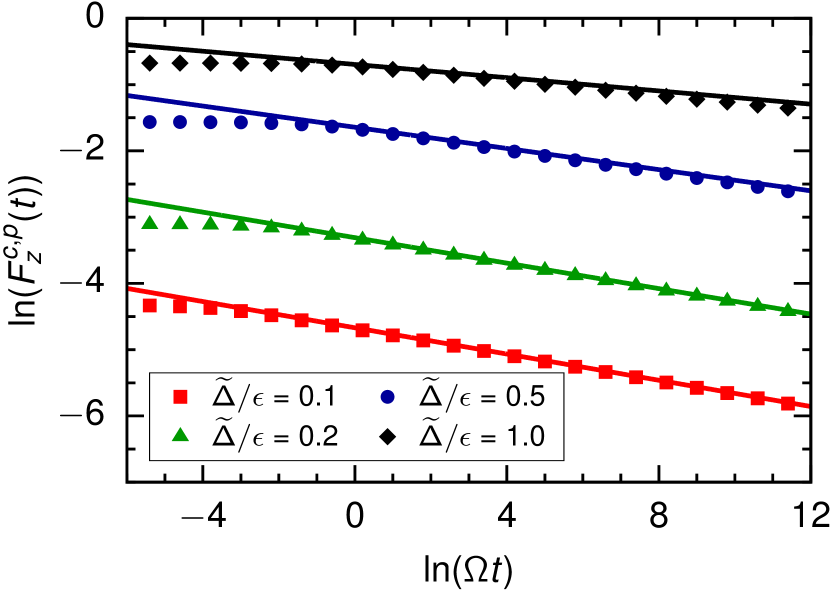
Figure 1: The numerical solution for the logarithm of the pole contribution $F_{z}^{c,p}(t)$ for $\alpha=0.05$, ${\langle\sigma_{z}\rangle}_{0}=1$, ${\langle\sigma_{x}\rangle}_{0}={\langle\sigma_{y}\rangle}_{0}=0$, and different values for $\tilde{\Delta}/\epsilon$ plotted as function of $\ln(\Omega t)$. For very large times a power-law appears with exponent $2\alpha\epsilon^{2}/\Omega^{2}$, in agreement with (404) (solid lines). The band width is chosen as $D/\Delta=10^{6}$.

V Summary

In this work we have presented the solution for the time dynamics of the ohmic spin boson model at finite bias by systematically expanding one order beyond Boch-Redfield. Using real-time RG and perturbation theory we have set up a renormalized perturbation theory to study analytically the whole time regime from exponentially small ($\Omega t\sim e^{-1/\alpha}$) up to large times ($\Omega t\gg 1$). For very large times we used the real-time RG method to sum up the leading logarithmic series in $\alpha\ln(\Omega t)$. As a result we obtained several interesting features for the time dynamics: (1) We showed how both the unrenormalized ($\Delta$) and renormalized tunneling ($\tilde{\Delta}$) enter the time dynamics and that it is not possible to account for the renormalization by using a local Hamiltonian with a renormalized tunneling. As in Ref. divincenzo_loss_05, we found that the renormalized Rabi frequency enters as high-energy cutoff scale to determine $\tilde{\Delta}$. (2) We found that all terms of the time evolution are exponentially damped by summing up all secular terms $\sim(\Gamma t)^{n}$. This results from a self-consistent perturbation theory in analogy to the one presented in Ref. slutskin_etal_11, . (3) For the preexponential functions of the oscillating modes and in the non-exponential time regime we found logarithmic terms $\sim\alpha\ln(\Omega t)$ containing the renormalized Rabi frequency as energy scale together with terms falling off as $\alpha/(\Omega t)$. (4) We showed that some correction terms in $O(\alpha)$ to Bloch-Redfield require an analysis of the Liouvillian up to second order in $\alpha$. We were able to calculate these terms by relating them to the stationary density matrix. (5) By resumming the leading logarithmic series in $\alpha\ln(\Omega t)$ in all orders of perturbation theory we found for the preexponential functions of the oscillating modes an interesting crossover from a power-law $\sim 1/(\Omega t)^{2\alpha}$ at exponentially small times to a power-law $\sim 1/(\Omega t)^{2\alpha{\epsilon^{2}\over\Omega^{2}}}$ at exponentially large times. The latter has also been proposed in Ref. slutskin_etal_11, but the logarithms determining the crossover to the power-law at small times have not been discussed there.

We have identified three important reasons why it is not sufficient to calculate the kernel of the kinetic equation up to first order in the coupling to the bath to obtain all terms of the first correction to the Bloch-Redfield result. We now discuss why these issues are quite generic and are expected to occur also for other models of dissipative quantum mechanics.

First, for times of the order of the inverse decay rate $t\sim\Gamma^{-1}$, where damping is still moderate, the distance of the Fourier variable $E$ to some of the poles $z_{i}$ of the propagator is proportional to the decay rate $|E-z_{i}|\sim\Gamma$. In this case perturbation theory is quite subtle since the denominator $E-L(E)$ of the propagator is of $O(\Gamma)$. The kernel $\Sigma(E)$ can no longer be considered as a small correction compared to $E-L_{0}$ and can not be expanded up to the numerator. We solved this problem by expanding all analytic parts of $\Sigma(E)$ around $E=z_{i}$ and keeping $\Sigma(z_{i})$ in the denominator whereas all other higher terms of the Taylor expansion are at least of $O(\alpha^{2})$ and can be taken as a small correction. The non-analytic terms of $\Sigma(E)$ are more subtle and are some function $f_{i}(E-z_{i})$ when $E$ is close to $z_{i}$, where $f_{i}(E)~{}\sim\alpha$ is a non-analytic function with branch cut on the negative imaginary axis. For the ohmic spin boson model we get $f_{i}(E-z_{i})\sim\alpha(E-z_{i})\ln(-i(E-z_{i}))\sim\alpha^{2}$ such that it can be considered as a small correction. For dissipative quantum models with logarithmic divergencies at high and low energies it is typical that $\Sigma(E)$ has a logarithmic form, see e.g. the Kondo model schoeller_reininghaus_09 or the interacting resonant level model RTRG_irlm , see Ref. schoeller_14, for a review. For weak coupling problems and $E$ close to $z_{i}$, $\Sigma(E)$ contains either logarithmic terms $\sim\ln(-i(E-z_{j}))$ with branching points $z_{j}\neq z_{i}$ (i.e. are analytic and can be expanded around $E=z_{i}$) or are proportional to $(E-z_{i})\ln(-i(E-z_{i}))$ (such that they vanish at $E=z_{i}$). Terms $\sim\Gamma\ln(-i(E-z_{i}))$ with a constant energy scale in front diverge at $E=z_{i}$ and are typical for strong coupling problems like e.g. the Kondo model. Most importantly, even for weak coupling problems, it is never allowed to expand any part of $\Sigma(E)$ in $\alpha$ by setting $z_{i}=z_{i}^{(0)}+\delta z_{i}$, where $z_{i}^{(0)}$ are the pole positions without the bath and $\delta z_{i}\sim O(\alpha)$ denotes the correction from the bath, since $(E-z_{i}^{(0)})/\delta z_{i}$ is a parameter of $O(1)$. Thus, for any model of dissipative quantum mechanics, it is very dangerous to use a naive perturbative expansion of the kernel in the coupling to the bath. The positions $z_{i}$ of the branching points of $L(E)$ (or poles of the propagator) should be kept non-perturbatively in a self-consistent way by using the full propagator and not the bare one between the vertices, as also emphasized in Ref. slutskin_etal_11, . For a non-interacting bath described by a quadratic form $H_{\text{bath}}=\sum_{q}\omega_{q}a_{q}^{\dagger}a_{q}$ in the field operators, the diagrammatic technique developed in Ref. schoeller_09, shows that all bare propagators can be replaced by full ones without any double counting such that a systematic self-consistent perturbation theory can be set up. Whether this is also possible for more complicated baths like e.g. spin baths is an open question.

Secondly, we have seen that degenerate perturbation theory is generically needed since the decay poles $z_{i}=-i\Gamma_{i}$ and the stationary pole $z_{\text{st}}=0$ of the propagator are close to each other within the decay rate $\Gamma_{i}\sim\alpha$. Therefore, second order terms are needed for the Liouvillian to calculate the stationary state and all terms of the time evolution of the purely decaying modes up to first order in $\alpha$. Again this problem occurs only for times of the order of the inverse decay rate, since for small times $|E-L_{0}|\sim 1/t$ is much larger than $\Gamma$ and can be considered as the largest term in the denominator of the propagator such that the full kernel $\Sigma(E)$ can be expanded up to the numerator. Thus, for two state models with one purely decaying and two oscillating modes, the complicated terms in the stationary state and the purely decaying mode arising from the second order terms of the Liouvillian, must generically cancel for small times. This simplifies the calculation of those terms for the purely decaying mode since they can be expressed via the stationary state which, for the equilibrium case, can be easily calculated up to first order in $\alpha$ via the partition function. This strategy has been taken over in this work by using the stationary state calculated in Ref. divincenzo_loss_05, up to $O(\alpha)$. However, for generic models with more than two local states, several purely decaying modes can occur and the problem of degenerate perturbation theory can no longer be solved by just calculating the first correction to Bloch-Redfield of the stationary state.

Whereas the two aforementioned issues are important to be considered for the calculation of the first correction to Bloch-Redfield on all time scales, there are further problems with weak coupling expansions in the regimes of exponentially small or large times. They arise for problems of dissipative quantum mechanics with logarithmic divergencies at high and low energies like the ohmic spin boson model, the interacting resonant level model, quantum dot models and the Kondo model. They have to be treated by an appropriate renormalization group method like the RTRG method schoeller_09 ; schoeller_14 . For weak coupling problems, where the renormalized vertices stay small in the whole complex plane, the RG equations can be truncated systematically such that logarithmic terms are summed up non-perturbatively in leading or subleading order. Whereas logarithmic divergencies at high energies can be incorporated in renormalized parameters from poor man scaling equations, logarithmic divergencies at low energies close to the branching points $z_{i}$ are quite subtle and require a full solution of the RG equations. For models of dissipative quantum mechanics without logarithmic divergencies this issue is not important.

Appendix A Liouvillian in perturbation theory

Here we calculate the Liouvillian up to first order in the coupling $\alpha$ to the bath by using the diagrammatic technique developped in Ref. kashuba_schoeller_13, , where an expansion in the coupling to the bath is used together with the application of Wick’s theorem to integrate out the phonon bath. In this reference it is shown for the ohmic spin boson model that the kernel $\Sigma(E)=\Sigma_{s}+\Sigma_{a}(E)$ can be split into two parts, one stemming from the symmetric and one from the antisymmetric part of the Bose distribution function of the bath. At zero temperature this leads to Eq. (24) with $\Sigma_{s}$ given by (30). The antisymmetric part $\Sigma_{a}(E)$ involves only the antisymmetric part of the Bose distribution $n(\omega)$ of the bath

$$n_{a}(\omega)\,=\,{1\over 2}(n(\omega)-n(-\omega))\,=\,{1\over 2}\text{sign}(\omega)$$ (405)

since $n(\omega)=-\theta(-\omega)$ at zero temperature. The lowest order diagram for

Figure 2: The lowest order diagram for the kernel $\Sigma_{a}(E)$. Here, the circles represent the bare vertices $G$, the black line connecting the vertices is the local propagator and the green line denotes the bath contraction.

$\Sigma_{a}(E)$ is shown in Fig. 2, where the green line indicates the contraction between the bath field operators which involves the spectral density (6) of the bath and the antisymmetric part of the Bose distribution function via

$$\gamma_{a}(\omega)\,=\,2\alpha\omega J_{c}(\omega)n_{a}(\omega)\,=\,\alpha|\omega|{D^{2}\over D^{2}+\omega^{2}}\quad.$$ (406)

Using the diagrammatic rules the diagram is translated as

$$\Sigma_{a}(E)\,=\,\int d\omega\gamma_{a}(\omega)GR_{a}(E+\omega)G\quad,$$ (407)

where $G$ is the bare vertex given by (348) and $R_{a}(E)=1/(E-L_{a}(E))$ is the local propagator of the antisymmetric part only. To approximate the $\omega$-dependence of $R_{a}(E+\omega)$, we exhibit the logarithmic parts by using the decomposition (45) and use the spectral decomposition (105-107) of $\tilde{L}_{\Delta}(E)$

$$R(E+\omega)\, =\,{1\over E+\omega-\tilde{L}_{\Delta}(E+\omega)}Z^{\prime}(E+\omega)$$

$$=\,\sum_{i}{1\over E+\omega-\lambda_{i}(E+\omega)}P_{i}(E+\omega)Z^{\prime}(E+\omega)\quad.$$ (408)

Neglecting the $\omega$-dependence of the logarithmic functions $\lambda_{i}(E+\omega)$, $P_{i}(E+\omega)$ and $Z^{\prime}(E+\omega)$ (leading to higher orders in $\alpha$), and using the integral (defined for $\text{Im}(E)>0$ and analytically continued into the lower half of the complex plane by choosing the branch cut along the direction of the negative imaginary axis)

$$\int d\omega|\omega|{D^{2}\over D^{2}+\omega^{2}}{1\over E+\omega}\, =\,{D^{2}\over D^{2}+E^{2}}2E\ln{-iE\over D}$$

$$\xrightarrow{D\rightarrow\infty}\,2E\ln{-iE\over D}\quad,$$ (409)

where $\ln(z)$ is the natural logarithm with branch cut on the negative real axis, we find from (407)

$$\Sigma_{a}(E)\,=\,2\alpha\sum_{i}{\cal{F}}_{i}(E)GP_{i}(E)Z^{\prime}(E)G\quad,$$ (410)

with ${\cal{F}}_{i}(E)$ defined in (36-37). Taking the projectors $P_{i}(E)$ and $Z^{\prime}(E)$ in lowest order, given by (137-143) and $Z^{\prime}(E)^{(0)}=1$, and inserting (348) for $G$, we find the result (33-35).

We note that the non-analytic features of $\Sigma_{a}(E)$ in the lower half of the complex plane are located at $E=z_{i}-ix$, $0<x<\infty$, where $z_{i}$ are the positions of the poles of $R_{a}(E)$. This holds exactly and can be shown in all orders of perturbation theory schoeller_09 ; schoeller_14 . E.g. for the lowest order diagram (407) we can see that this holds even when we do not use any approximation for the $\omega$-dependence of $R_{a}(E+\omega)$. Closing the integration contour in the upper half and noting that $R_{a}(E+\omega)$ is an analytic function there and $\gamma_{a}(E)$ has non-analytic features only on the imaginary axis, we find the result

$$\Sigma(E)\, =\,i\int_{0}^{\infty}dx\Big{\{}\gamma_{a}(ix+0^{+})-\gamma_{a}(ix-0^{+})\Big{\}}\cdot$$

$$\hskip 56.9055pt\cdot GR_{a}(E+ix)G\quad.$$ (411)

Since $R_{a}(E+ix)$ has a pole at $E+ix=z_{i}$, we find that $\Sigma(E)$ is non-analytic for $E=z_{i}-ix$ with $0<x<\infty$. A similar proof can be used to show this in all orders of perturbation theory, see Ref. schoeller_09, ; schoeller_14, .

Furthermore, we note that the matrix structure

$$\Sigma_{a}(E)\,=\,\left(\begin{array}[]{cc}0&0\\ 0&\hat{\Sigma}_{a}(E)\end{array}\right)$$ (414)

holds in all orders of perturbation theory. This is due to the fact that the bare vertices $G$ have the same structure, see (348), and for each diagram all intermediate propagators are sandwiched between two vertices. A consequence of this matrix structure is that the projector $P_{\text{st}}$ on the zero eigenvalue of $\tilde{L}_{\Delta}(E)$ is exactly known and given by (118).

Appendix B Projectors for $\tilde{L}_{0}+\tilde{\Sigma}_{a}^{i}$

To calculate the projectors of the matrix $\tilde{L}_{0}+\tilde{\Sigma}_{a}^{i}$ up to $O(\alpha)$, we first set up the matrix $\tilde{\Sigma}_{a}^{i}=\tilde{\Sigma}_{a}(z_{i})$ by setting $E=z_{i}$ in (69) and use

$${\cal{F}}_{0}(0)\,\sim\,O(\alpha)\quad,\quad{\cal{F}}_{0}(z_{0})\,=\,{\cal{F}}_{\sigma}(z_{\sigma})\,=\,0\quad,$$

$${\cal{F}}_{\sigma}(0)\,,\,{\cal{F}}_{\sigma}(z_{0})\,,\,{\cal{F}}_{0}(z_{\sigma})\,=\,-i{\pi\over 2}\Omega+O(\alpha)\quad,$$

$${\cal{F}}_{-\sigma}(z_{\sigma})\,=\,2\sigma\Omega\ln{2}-i\pi\Omega+O(\alpha)\quad,$$ (415)

This gives for $\tilde{\Sigma}_{a}^{i}$ transformed with the matrix $A$ (see (198)) up to $O(\alpha)$ the result

$$A\tilde{\Sigma}_{a}^{\text{st}}A\, =\,A\tilde{\Sigma}_{a}^{0}A\,=\,-i\pi\alpha{1\over\Omega}\left(\begin{array}[]{cc}\tilde{\Delta}^{2}\tau_{-}&\Delta\epsilon\tau_{-}\sigma_{z}\\ {\tilde{\Delta}^{2}\over\Delta}\epsilon\sigma_{z}\tau_{-}&\epsilon^{2}\end{array}\right)\quad,$$ (418)

$$A\tilde{\Sigma}_{a}^{\sigma}A\, =\,-i\pi\alpha{\tilde{\Delta}^{2}\over\Omega}\left(\begin{array}[]{cc}0&0\\ 0&\tau_{-}\end{array}\right)\,+\,$$ (421)

$$\,+\,\alpha{1\over\Omega}a_{\sigma}\left(\begin{array}[]{cc}\tilde{\Delta}^{2}\tau_{-}&\Delta\epsilon\tau_{-}(\sigma_{z}-\sigma)\\ {\tilde{\Delta}^{2}\over\Delta}\epsilon(\sigma_{z}-\sigma)\tau_{-}&\epsilon^{2}(1-\sigma\sigma_{z})\end{array}\right)\quad,$$ (424)

where $a_{\sigma}=2\sigma\ln{2}-i\pi$. The transformed Liouvillian $A\tilde{L}_{0}A$ is given by (201). Due to the matrix structure of $\tilde{\Sigma}_{a}(E)$, one projector is exactly known (in all orders of perturbation theory, see (118) and (414))

$$A\tilde{P}^{i}_{\text{st}}A\, =\,\left(\begin{array}[]{cc}\tau_{+}&0\\ 0&0\end{array}\right)\quad.$$ (427)

Using usual perturbation theory it is straightforward to calculate the projectors $\tilde{P}_{\sigma}^{\text{st},0,\sigma}$ in zero and first order in $\alpha$ as

$$A\tilde{P}^{(0)i}_{\sigma}A\, =\,{1\over 2}\left(\begin{array}[]{cc}0&0\\ 0&1+\sigma\sigma_{z}\end{array}\right)\quad,$$ (430)

$$A\tilde{P}^{(1)\text{st},0}_{\sigma}A\, =$$

$$=\,-{1\over 2}i\pi\alpha{\tilde{\Delta}^{2}\epsilon\over\Delta\Omega^{2}}\left(\begin{array}[]{cc}0&{1\over Z}\tau_{-}(1+\sigma\sigma_{z})\\ (1+\sigma\sigma_{z})\tau_{-}&0\end{array}\right)\quad,$$ (433)

$$A\tilde{P}^{(1)\sigma}_{\sigma}A\, =\,{1\over 4}i\pi\sigma\alpha{\tilde{\Delta}^{2}\over\Omega^{2}}\left(\begin{array}[]{cc}0&0\\ 0&\tau_{+}-\tau_{-}\end{array}\right)\quad.$$ (436)

Using $\sum_{j=\text{st},0,\pm}A\tilde{P}_{j}^{i}A=1$, we find

$$A\tilde{P}^{(0)i}_{0}A\, =\,\left(\begin{array}[]{cc}\tau_{-}&0\\ 0&0\end{array}\right)\quad,$$ (439)

$$A\tilde{P}^{(1)\text{st},0}_{0}A\, =\,i\pi\alpha{\tilde{\Delta}^{2}\epsilon\over\Delta\Omega^{2}}\left(\begin{array}[]{cc}0&{1\over Z}\tau_{-}\\ \tau_{-}&0\end{array}\right)\quad.$$ (442)

This proves (224-233) and (278-287). We note that although degenerate perturbation theory is needed to calculate $\tilde{P}_{0}^{i}$ up to first order in $\alpha$, we do not need any second order terms in $\alpha$ for the Liouvillian since the projector $\tilde{P}_{\text{st}}^{i}$ is exactly known. This is a particular advantage for the spin boson model.

To derive the formula (274) for the eigenvalue $\tilde{\gamma}_{0}^{\text{st}}$ of $\tilde{L}_{a}(0)$ up to second order in $\alpha$, we relate it to the eigenvalue $\tilde{\gamma}_{0}^{0}=z_{0}=-i(\Gamma^{(1)}+\Gamma^{(2)}+O(\alpha^{3}))$ of $\tilde{L}_{a}(z_{0})$. We first note that, due to the matrix structure of $A\tilde{L}_{a}^{\text{st},0}A$ (see (201) and (418)), the second order contribution to the eigenvalues $\tilde{\gamma}_{0}^{\text{st},0}$ is not influenced by the non-diagonal blocks of $A\tilde{L}_{a}^{\text{st},0}A$ and arises only from the upper left block. Denoting this block by $(A\tilde{L}_{a}^{\text{st},0}A)_{11}$ we expand

$$\tilde{L}_{a}(0)_{11}\,=\,\tilde{L}_{a}(z_{0})_{11}\,-\,{d\tilde{\Sigma}_{a}\over dE}(0)_{11}z_{0}\,+\,O(\alpha^{3})\quad.$$ (443)

and use (69) together with ${d\over dE}{\cal{F}}_{\sigma}(0)=1+i\sigma{\pi\over 2}+O(\alpha)$ to get

$$\tilde{L}_{a}(0)_{11}\,=\,\tilde{L}_{a}(z_{0})_{11}\,+\,2i\Gamma^{(1)}\alpha{\tilde{\Delta}^{2}\over\Omega^{2}}\tau_{-}\,+\,O(\alpha^{3})\quad,$$ (444)

such that

$$\tilde{\gamma}_{0}^{\text{st}}\,=\,z_{0}\,+\,2i\Gamma^{(1)}\alpha{\tilde{\Delta}^{2}\over\Omega^{2}}\,+\,O(\alpha^{3})\quad,$$ (445)

which proves (274).

References

• (1) A.J. Leggett, S. Chakravarty, T.A. Dorsey, M.P.A. Fisher, A. Garg, and W. Zwerger, Rev. Mod. Phys. 59, 1 (1987).
• (2) U. Weiss, Quantum Dissipative Systems (World Scientific Publishing Company, Singapore, 2012).
• (3) M. Grifoni and P. Haenggi, Phys. Rep. 304,229 (1998).
• (4) A. Hutter and D. Loss, Phys. Rev. A 89, 042334 (2014).
• (5) E. Novais and E.R. Mucciolo, Phys. Rev. Lett. 110, 010502 (2013).
• (6) M. Pletyukhov, D. Schuricht, and H. Schoeller, Phys. Rev. Lett. 104, 106801 (2010).
• (7) H. Schoeller, Eur. Phys. J. Spec. Top. 168, 179 (2009).
• (8) H. Schoeller, “Dynamics of open quantum systems”, in Lecture Notes of the 45th IFF Spring School “Computing Solids - Models, ab-initio methods and supercomputing” (Forschungszentrum Jülich, 2014).
• (9) M. Pletyukhov and H. Schoeller, Phys. Rev. Lett. 108, 260601 (2012).
• (10) L. van Hove, Physica 21, 517 (1955); D. Loss, Physica A 139, 505 (1986).
• (11) A. A. Slutskin et al., Europhys. Lett. 96, 40003 (2011).
• (12) O. Kashuba and H. Schoeller, Phys. Rev. B 87, 201402(R) (2013).
• (13) D.P. DiVincenzo and D. Loss, Phys. Rev. B 71, 035318 (2005).
• (14) R. Egger, H. Grabert, and U. Weiss, Phys. Rev. E 55, R3809 (1997).
• (15) D. M. Kennes, O. Kashuba, M. Pletyukhov, H. Schoeller, and V. Meden, Phys. Rev. Lett. 110, 100405 (2013).
• (16) H. Mori, Progress of Theoretical Physics 33, 423 (1965); H. Grabert, Projection Operator Techniques in Nonequilibrium Statistical Mechanics, 1st ed., Springer Tracts in Modern Physics, Vol. 95 (Springer, Berlin, 1982) p. 166; E. Fick and G. Sauermann, The Quantum Statistics of Dynamic Processes (Springer Series in Solid-State Sciences 86, Springer-Verlag, Berlin, 1990); C. W. Gardiner, Quantum Noise (Springer Series in Synergetics 56, Springer-Verlag, Berlin, 1991); R. Zwanzig, Nonequilibrium Statistical Mechanics, 3rd ed. (Oxford University Press, New York, 2001) p. 240.
• (17) H. Schoeller and F. Reininghaus, Phys. Rev. B 80, 045117 (2009); ibid. Phys. Rev. B 80, 209901(E) (2009).
• (18) C. Karrasch, S. Andergassen, M. Pletyukhov, D. Schuricht, L. Borda, V. Meden, and H. Schoeller, Europhys. Lett. 90, 30003 (2010); S. Andergassen, M. Pletyukhov, D. Schuricht, H. Schoeller, and L. Borda, Phys. Rev. B 83, 205103 (2011).