Lepton-flavour-violating gluonic operators:

Abstract

Effective operators provide a model-independent description of physics beyond the standard model that is particularly useful given the absence of any signs of new physics at the Large Hadron Collider (LHC). We recast previous LHC analyses to set limits on lepton-flavour-violating gluonic effective operators of dimension 8 and compare our results to existing limits from low-energy precision experiments. Current LHC data constrains the scale $\Lambda$ of the effective operators to be larger than $\Lambda\gtrsim 0.5-1.6$ TeV depending on the flavour and thus provides the most stringent limit for all operators apart from parity-conserving operators of the form $GG\,\bar{\mu}P_{L,R}e$, where $\mu$-$e$ conversion in nuclei poses the most stringent constraint.

1 Introduction

The Large Hadron Collider (LHC) successfully discovered the 125 GeV Higgs boson in 2012 [1, 2] and thus confirmed the last missing piece of the Standard Model (SM). However there are several hints for physics beyond the SM. In particular the observation of neutrino oscillations [3] (and consequently the existence of massive neutrinos) showed that lepton flavour is not conserved and lepton-flavour-violating (LFV) processes exist. In particular charged leptons may change flavour in processes such as radiative muon decay $\mu\to e\gamma$. In minimal models of neutrino mass for Dirac neutrinos, such as the SM augmented by the Weinberg operator [4] or the seesaw model [5], the rates for LFV processes are tiny, because they are suppressed by the smallness of the neutrino mass. This is no longer true in more general models, and there are many well-motivated models such as seesaw models with electroweak triplets [6, 7] or radiative neutrino mass models [8, 9, 10] (See Ref. [11] for a recent review.) in which charged LFV processes are important. More generally, there are many known extensions of the SM which do not conserve lepton flavour and can be tested by studying LFV processes at the LHC. Examples include ($R$-parity violating) supersymmetric models [12] and $Z^{\prime}$ models [13].

Low-energy precision experiments including MEG [14], SINDRUM [15] and the B-factories BaBar [16] and Belle [17] have searched for charged LFV processes and placed severe constraints on many LFV processes. At the same time, the LHC experiments are currently pushing the limits for the scale of any new physics higher and higher. Effective field theory (EFT) is the ideal framework to describe new LFV processes under these conditions. Existing studies have mostly focused on the leading dimension six effective operators with two quarks and two leptons. Ref. [18] derived constraints from rare decays and from collider bounds on contact interactions. Ref. [19] focused on LHC constraints finding they can be competitive to those from rare processes. In particular effective LFV operators with two leptons of different flavour and two coloured particles, quarks and gluons, provide a clean signature with low SM background and large production cross section at the LHC, and this has been exploited in Ref. [19] to extract competitive constraints for operators with right-handed $\tau$-leptons. Ref. [20] suggested to use $pp\to\mu^{\pm}\tau^{\mp}t\bar{t}$ to probe operators with top quarks and Ref. [21] studied the channel $pp\to\mu^{\pm}\tau^{\mp}jj$ to search for heavy singlet neutrinos in the inverse seesaw model. LFV operators with gluons may also be probed in a lepton-hadron collider via the process $\ell g\to\ell^{\prime}g$ [22].

In this study we focus on LFV gluonic dimension-8 operators, with two leptons of different flavour coupled to two gluons. Although technically in the EFT they are suppressed with respect to dimension-6 operators, this suppression is compensated by the large gluon content of protons at high energies [23]. Low-energy precision constraints on these operators have been previously studied in Ref. [24]. We derive LHC limits and compare them to the updated low-energy constraints.

The paper is structured as follows: in Sec. 2 we introduce the dimension-8 operators and fix the notation. Possible ultraviolet (UV) completions are discussed in Sec. 3. In Sec. 4 we discuss LFV signals at the LHC and recast existing LHC analyses to obtain a limit on the scale of each operator, which forms the main result of our study. Sec. 5 provides a brief summary of the relevant low-energy precision constraints. Finally we summarise in Sec. 6 and compare the sensitivity of LHC searches with low-energy precision experiments.

2 Effective LFV gluonic dimension-8 operators

There are six independent operators for one flavour of leptons (54 for three flavours) with two gluon field strength tensors and two leptons [25, 26]. The effective Lagrangian with these operators can thus be written as follows

$$\mathcal{L} =x_{ij}\mathcal{O}^{ij}_{X}+x^{\prime}_{ij}\mathcal{O}^{\prime ij}_{X}+\bar{x}_{ij}\bar{\mathcal{O}}^{ij}_{X}+\bar{x}^{\prime}_{ij}\bar{\mathcal{O}}^{\prime ij}_{X}+y_{ij}\,\mathcal{O}^{ij}_{Y}+z_{ij}\,\mathcal{O}^{ij}_{Z}$$ (1)

where the Wilson coefficients $x$, $x^{\prime}$, $\bar{x}$ and $\bar{x}^{\prime}$ are real matrices and $y$ and $z$ Hermitian matrices in flavour space and the operators are defined as

$$\mathcal{O}^{ij}_{X} =\alpha_{s}G_{\mu\nu}^{a}G^{a\mu\nu}\left(\bar{e}_{Ri}L_{j}\cdot\phi^{*}+\bar{L}_{j}\cdot\phi e_{Ri}\right) \mathcal{O}^{\prime ij}_{X} =i\,\alpha_{s}G_{\mu\nu}^{a}\tilde{G}^{a\mu\nu}\left(\bar{e}_{Ri}L_{j}\cdot\phi^{*}-\bar{L}_{j}\cdot\phi e_{Ri}\right)$$ (2a)

$$\bar{\mathcal{O}}^{ij}_{X} =i\,\alpha_{s}G_{\mu\nu}^{a}G^{a\mu\nu}\left(\bar{e}_{Ri}L_{j}\cdot\phi^{*}-\bar{L}_{j}\cdot\phi e_{Ri}\right) \bar{\mathcal{O}}^{\prime ij}_{X} =\alpha_{s}G_{\mu\nu}^{a}\tilde{G}^{a\mu\nu}\left(\bar{e}_{Ri}L_{j}\cdot\phi^{*}+\bar{L}_{j}\cdot\phi e_{Ri}\right)$$ (2b)

$$\mathcal{O}^{ij}_{Y} =i\,\alpha_{s}G_{\mu\rho}^{a}G_{\sigma\nu}^{a}\eta^{\rho\sigma}\bar{L}_{i}\gamma^{\mu}D^{\nu}L_{j} \mathcal{O}^{ij}_{Z} =i\,\alpha_{s}G_{\mu\rho}^{a}G_{\sigma\nu}^{a}\eta^{\rho\sigma}\bar{e}_{Ri}\gamma^{\mu}D^{\nu}e_{Rj}\;.$$ (2c)

$G_{\mu\nu}$ denotes the gluon field strength tensor and its dual $\tilde{G}_{\mu\nu}=\tfrac{1}{2}\epsilon_{\mu\nu\rho\sigma}G^{\rho\sigma}$. The SM Higgs doublet is denoted as $\phi$, the left-handed lepton doublet $L$ and the right-handed charged leptons $e_{R}$. $D_{\nu}$ is the covariant derivative. All operators are normalised with the strong coupling $\alpha_{s}\equiv g_{s}^{2}/4\pi$. The normalisation is chosen such that the operators with Wilson coefficients $x$, $x^{\prime}$, $\bar{x}$ and $\bar{x}^{\prime}$ in the first two lines are invariant under QCD corrections at one-loop order (See e.g. [27]). We only consider low-energy constraints for these operators in Sec. 5, because operators with derivatives are further suppressed at low energy. The combination of gluon field strength tensors $G_{\mu\nu}^{a}\tilde{G}^{a\mu\nu}$ in the primed operators $\mathcal{O}_{X}^{\prime}$ and $\bar{\mathcal{O}}_{X}^{\prime}$ violates parity which is important for low-energy constraints. The operators with an over-bar $\bar{\mathcal{O}}_{X}^{(\prime)}$ violate CP. Thus imposing CP results in $\bar{x}_{ij}=\bar{x}^{\prime}_{ij}=0$.

The operators in Eq. 2 are defined in the weak interaction basis. We obtain the relevant interactions after a rotation of the charged leptons $e_{L,R}$ to the mass basis $\hat{e}_{L,R}$ and the corresponding rotation of the neutrino weak interaction eigenstates $\nu_{L}$

$$e_{L} =L_{e}\hat{e}_{L} e_{R} =R_{e}\hat{e}_{R} \nu_{L} =L_{e}\hat{\nu}_{L}\;.$$ (3)

For simplicity we choose $L_{e}=R_{e}=1$ without loss of generality and drop the hats on the fields. In this case the leptonic mixing entirely originates from the neutrino sector. Thus the interactions of two charged leptons with two gluons are simply given by

$$\mathcal{L} =\frac{\alpha_{s}vx_{ij}}{\sqrt{2}}\,G_{\mu\nu}^{a}G^{a\mu\nu}\left(\bar{{e}}_{Ri}e_{Lj}+\bar{{e}}_{Lj}{e}_{Ri}\right)+\frac{i\alpha_{s}vx^{\prime}_{ij}}{\sqrt{2}}\,G_{\mu\nu}^{a}\tilde{G}^{a\mu\nu}\left(\bar{{e}}_{Ri}e_{Lj}-\bar{e}_{Lj}{e}_{Ri}\right)$$

$$+\frac{i\alpha_{s}v{\bar{x}}_{ij}}{\sqrt{2}}\,G_{\mu\nu}^{a}G^{a\mu\nu}\left(\bar{{e}}_{Ri}e_{Lj}-\bar{{e}}_{Lj}e_{Ri}\right)+\frac{\alpha_{s}v{\bar{x}}^{\prime}_{ij}}{\sqrt{2}}\,G_{\mu\nu}^{a}\tilde{G}^{a\mu\nu}\left(\bar{{e}}_{Ri}e_{Lj}+\bar{{e}}_{Lj}e_{Ri}\right)$$ (4)

$$+\frac{i\alpha_{s}vy_{ij}}{\sqrt{2}}\,G_{\mu\rho}^{a}G_{\sigma\nu}^{a}\eta^{\rho\sigma}\bar{{e}}_{Li}\gamma^{\mu}D^{\nu}{e}_{Lj}+\frac{i\alpha_{s}vz_{ij}}{\sqrt{2}}\,G_{\mu\rho}^{a}G_{\sigma\nu}^{a}\eta^{\rho\sigma}\bar{e}_{Ri}\gamma^{\mu}D^{\nu}e_{Rj}$$

with $\left\langle\phi\right\rangle=(0\;v)^{T}/\sqrt{2}$ and the electroweak vacuum expectation value $v\simeq 246$ GeV.

3 UV completions

In this section we discuss possible models giving rise to the effective operators of the previous section. Dimensional arguments suggest, as usual, that the largest coefficients would appear in models that produce the operators at tree-level. The operators in Eqs. (2a) and (2b) can be produced by the s-channel exchange of a spin zero particle in $gg\to\ell\ell^{\prime}$, whereas those in Eqs. (2c) would be produced by the exchange of a spin two particle in the s-channel of the same process. The two gluons are respectively in a spin zero or two configuration in these processes.

(a) Heavy Higgs and heavy quarks integrated out

$\implies$

(b) Heavy vector leptoquark and heavy quarks integrated out

Figure 1: Examples of UV completions of dimension-8 operators with two gluon field strength tensors and two leptons.

The spin zero operators are produced by a scalar exchange in the s-channel as shown schematically in Fig. 1(a). They can also be produced by a leptoquark exchange as illustrated in Fig. 1(b) [23]. The simplest UV completion scenario is a multi-Higgs model. The process in Fig. 1(a) would start from the one-loop production of a heavy neutral Higgs from gluon fusion which is dominated by the contributions of heavy quarks $Q$. This vertex is proportional to known loop factors and mixing angles in the scalar sector. The loop factor (indicated in the figure as $I(m_{H}^{2}/(4m_{Q}^{2})$) is known to be of order one in the range $m_{H}\lesssim 2m_{Q}$ [28]. The amplitude is not suppressed by powers of $m_{Q}$ provided that the $HQQ$ coupling is proportional to $m_{Q}$. An example of a model with the necessary ingredients is that of Refs. [29, 30, 31]. In this case the heavy neutral scalar gives mass to the fourth generation quarks running in the loop, we assume two of them for the factor of 2 in Eq. (5). The second ingredient necessary for this process to occur is a LFV coupling to the heavy scalar. Such couplings are generic to multi-Higgs models unless they are specifically removed with the use of discrete symmetries. They have been studied recently in the context of the $h\to\mu\tau$ limit set by CMS [32, 33] in a variety of multi-scalar models [34, 35, 36, 37, 38, 39]. In the notation of Ref. [31], the Wilson coefficients are generically given by

$$x_{ij}\sim\frac{8\pi}{3}\left(\frac{1}{4\pi v}\right)^{2}\frac{1}{m_{H}^{2}}\left(\frac{\cos\alpha\sin\beta}{\sin 2\beta}\right)^{2}\sin(\beta-\alpha)\Sigma^{\ell}_{ij}\frac{m_{\ell}}{v}.$$ (5)

The different factors involving $\alpha,\beta$ represent mixing in the scalar sector of the model, $\Sigma^{\ell}_{ij}$ encodes the LFV Yukawa coupling of the heavy scalar and $m_{\ell}$ is a generic lepton mass associated with the latter. The high energy scales suppressing this operator can thus be as low as $\Lambda^{4}\sim m_{H}^{2}(4\pi v)^{2}$ in this case.

The spin zero operators can also be produced by a leptoquark as illustrated in Fig. 1(b). The size of this contribution can be estimated as follows: if the leptoquark (scalar or vector) is very heavy, part of the diagram can be contracted to a four-fermion interaction as indicated in the figure. This four-fermion interaction can then be Fierz re-arranged to obtain the $\bar{Q}Q\bar{\ell}\ell^{\prime}$ structure. At this point the diagram looks like the heavy scalar exchange diagram and produces similar results provided the same approximations hold. This requires heavy fermions in the loop (heavier than the top-quark) and the condition $\hat{s}\lesssim 4m_{Q}^{2}$ for the loop factor to be of order 1. The Fierz rearrangement also produces the structure $\bar{Q}\gamma_{5}Q\bar{\ell}\gamma_{5}\ell^{\prime}$ which makes the diagram behave like an exchange of a heavy pseudo-scalar and produce the $x^{\prime}_{ij}$ coefficients. An example of a model with the required ingredients can be found in the discussion of heavy vector-like quarks of Ref. [40] which would yield

$$x_{ij}\sim x^{\prime}_{ij}\sim\frac{\pi}{3}\left(\frac{1}{4\pi v}\right)^{2}\frac{1}{m_{X}^{2}}\lambda_{\chi}^{2}\frac{v^{2}}{m_{Q}m_{\ell}}$$ (6)

where $\lambda_{\chi}$ is the Yukawa interaction between the (scalar) leptoquark, the heavy vector-like quark, and the lepton and it could be of order one. The last factor rescales this diagram to the one produced by a heavy Higgs.

Finally, the spin two operators can be produced by the tree-level exchange of a spin two resonance. One possibility is a composite analogue to the $f_{2}$ or $a_{2}$ resonances that occur in the strong interaction. A second possibility discussed in the literature is the exchange of Kaluza-Klein (KK) states [41] where we can read directly from Eq. (71) of this reference that, for example for $n=3$,

$$y_{ij}=z_{ij}=\frac{8\pi}{\alpha_{s}M_{S}^{4}}\delta_{ij}.$$ (7)

KK states would only produce parity and flavour conserving operators so they are not directly relevant for our study, but they illustrate how the operators may arise in a more complicated model.

4 LFV signals at the LHC

The operators listed in Eq. (2) also produce distinctive signals with flavour violating (charged) lepton pairs at hadron colliders. We consider one operator at a time. Obviously in realistic UV completions multiple operators are generically produced at the same time, but the constraints in the ”one-operator-at-a-time” approach also provide a good and simple estimate for the general strength of the constraints.

In the case where no spin correlations are observed, the spin averaged matrix elements squared produced by these operators are given by

$$\overline{|\mathcal{M}_{X^{(\prime)}}|^{2}} \sim\alpha_{s}^{2}|x_{ij}^{(\prime)}|^{2}v^{2}\hat{s}^{3} \overline{|\mathcal{M}_{{\bar{X}}^{(\prime)}}|^{2}} \sim\alpha_{s}^{2}|\bar{x}_{ij}^{(\prime)}|^{2}v^{2}\hat{s}^{3}$$ (8)

for the operators without derivatives. The ratio of their cross sections are simply given by the ratio of the squared Wilson coefficients. The derivative operators on the other hand are more sensitive to the center of mass energy and scale like

$$\overline{|\mathcal{M}_{Y}|^{2}} \sim\alpha_{s}^{2}|y_{ij}|^{2}\hat{s}^{4} \overline{|\mathcal{M}_{Z}|^{2}} \sim\alpha_{s}^{2}|z_{ij}|^{2}\hat{s}^{4}\;.$$ (9)

Again the ratio of the cross sections is given by $\sigma_{Y}/\sigma_{Z}=|y_{ij}|^{2}/|z_{ij}|^{2}$. This indicates that LHC limits cannot distinguish between the first four types of operators $\mathcal{O}_{X}^{(\prime)}$ and $\bar{\mathcal{O}}_{X}^{(\prime)}$ or between the last two, and that the LHC should be more sensitive to the latter ones. We quote all limits in terms of the scale $\Lambda$ of the operators which is given by the inverse of the fourth root of each Wilson coefficient, e.g. $\Lambda=x^{-1/4}$ for the operator $\mathcal{O}_{X}$.

For final states with $e\mu$ pairs, CMS has recently updated their analysis [42] based on a data set of 35.9 fb^-1 at $\sqrt{s}=13$ TeV, which has improved the limits reported by ATLAS previously in Ref. [43]. For $e\tau$ and $\mu\tau$ final states, however, the ATLAS search [43] still places the most stringent limit with 3.2 fb^-1 data at $\sqrt{s}=$13 TeV.

The signal samples are generated at parton level with MadGraph5_aMC@NLO [44] and subsequently processed with PYTHIA 8 for shower and hadronization [45]. Note that no next-to-leading order factors are included and the limits presented here are conservative. A fast detector simulation is performed using Delphes [47] with the default CMS configuration for $e\mu$ final states and the ATLAS one for $e\tau$ and $\mu\tau$ final states.

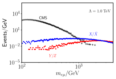
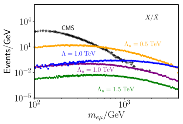
Figure 2: The invariant mass distribution of selected $e\mu$ pairs for the signals together with CMS data shown in black. With $\Lambda=1$ TeV and no unitarisation, signals in the left panel are in blue for $\mathcal{O}_{X}^{(\prime)}$, $\bar{\mathcal{O}}_{X}^{(\prime)}$ and in red for $\mathcal{O}_{Y,Z}$. In the right panel, signals for operator $\mathcal{O}_{X}$ at $\Lambda=1$ TeV without unitarisation and $\Lambda_{u}=0.5$, $1$ and $1.5$ TeV with unitarisation are shown in orange, purple and green respectively.

In the left panel of Fig. 2 we show the predicted invariant mass distribution of $e\mu$ pairs at the reconstruction level together with the data from CMS in black for operators $\mathcal{O}_{X}^{(\prime)}$, $\bar{\mathcal{O}}_{X}^{(\prime)}$ and $\mathcal{O}_{Y,Z}$ in blue and red respectively with $\Lambda=1$ TeV in the simple EFT. Note that the cross section is strictly proportional to $\Lambda^{-8}$ in this case and the shape of the distribution does not change. So it is straightforward to derive the lower limit on $\Lambda$ from the upper limit on the production cross section for simple EFTs. Clearly the distribution of the signal does not decline as fast as the SM background in the high energy region due the enhancement from the derivatives in the operators.

As is well known the EFT calculation eventually violates perturbative unitarity at some energy and become an obvious over-prediction of the rate. This can be a problem in calculations for the LHC, where the parton distribution functions (PDF’s) allow the process to probe energies as large as $\sqrt{s}$, albeit with decreasing probability. To address this issue, we follow the ad-hoc prescription described in Ref. [48] and replace the couplings of the effective operators by a form factor

$$C\to\frac{C}{1+\tfrac{\hat{s}}{\Lambda^{\prime 2}}}$$ (10)

where $\Lambda^{\prime}$ is an arbitrary scale which we choose to be equal to the scale $\Lambda$ of the operator. This ensures that the predicted cross sections do not violate perturbative unitarity anywhere and leads to meaningful limits on the effective operators. In the following we denote the scale of the operator in the unitarised EFT by $\Lambda_{u}$ and the scale of the operator in the simple EFT by $\Lambda$. In the right panel of Fig. 2, we show the invariant mass distribution for operators $\mathcal{O}_{X}$ without unitarisation at $\Lambda=1$ TeV in blue and with unitarisation at $\Lambda_{u}=0.5$, $1$ and $1.5$ TeV in orange, purple and green, respectively.

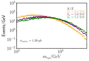
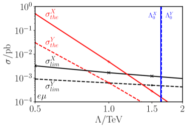
Figure 3: Left: The invariant mass distribution of selected $e\mu$ pairs for $\mathcal{O}_{X}^{(\prime)}$, $\bar{\mathcal{O}}_{X}^{(\prime)}$ with $\Lambda_{u}=0.5$, $1$ and $1.5$ TeV normalised to the same cross section. Right: The blue solid (dashed) line shows the upper limit on the production cross section at $95\%$ C.L. for the operator $\mathcal{O}_{X}$ ($\mathcal{O}_{Y}$) in the simple EFT. The red solid (dashed) line denotes the predicted cross section for the operator $\mathcal{O}_{X}$ ($\mathcal{O}_{Y}$) in the unitarised EFT. The upper limit in the unitarised EFT is shown as a black solid (dashed) line for the operator $\mathcal{O}_{X}$ ($\mathcal{O}_{Y}$). The lower limit on $\Lambda_{u}$ is the intersection of the red and black lines.

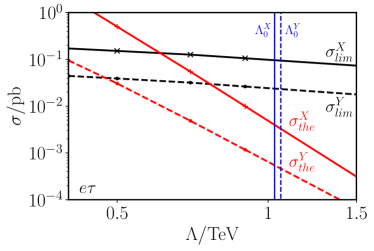
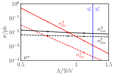
Figure 4: The colours of the lines are the same as in the right part of Fig. 3. Left: Operators with flavours $e\tau$. Right: Operators with flavours $\mu\tau$. The limits for the simple EFT lie on top of each other. Note the different ranges for $\Lambda$.

The CMS data is shown in black again. Compared with the simple EFT without unitarisation, the high energy tail of the distribution is tamed as it should be. If we further increase $\Lambda_{u}$ to 1.5 TeV or larger we are increasing the scale of the operator affecting the result in two ways: the production cross section decreases; but there are relatively more high energy events as shown in Fig. 3. In this case the distribution is changing with $\Lambda_{u}$ and in order to derive the constraints we need to vary $\Lambda_{u}$ until the predicted cross section matches the upper limit derived from the distribution.

	$\Lambda$ [TeV]		$\Lambda_{u}$ [TeV]
	$\mathcal{O}_{X}^{(\prime)}$, $\bar{\mathcal{O}}_{X}^{(\prime)}$	$\mathcal{O}_{Y,Z}$	$\mathcal{O}_{X}^{(\prime)}$, $\bar{\mathcal{O}}_{X}^{(\prime)}$	$\mathcal{O}_{Y,Z}$
$e\mu$	1.63	1.64	1.17	0.98
$e\tau$	1.03	1.06	0.61	0.47
$\mu\tau$	1.23	1.23	0.90	0.67

Table 1: Lower limits on the scale for various operators with ($\Lambda_{u}$) and without ($\Lambda$) unitarisation.

To derive the lower limit on $\Lambda$, we first construct the negative log likelihood function assuming the number of events in each bin follows a Poisson distribution while the errors follow a Gaussian distribution. Both the data and the background distributions are taken from the experimental papers [42, 43]. Then the profiled likelihoods are calculated taking the errors as nuisance parameters. The upper limit on the production cross section at 95% confidence level (C.L.) corresponding to a specific shape of distribution is achieved at $\Delta(-2\ln L)=3.84$ from the minimum of the negative log likelihood. With the upper limits derived, the lower limit on $\Lambda$ in the simple EFT without unitarisation can be easily calculated. For the unitarised case, we need to vary $\Lambda_{u}$ to find where the predicted production cross section just meets the upper limit on the cross section for the corresponding shape of distribution as shown in Fig. 3. We find CMS can exclude scales $\Lambda$ of the operators below 1.63 and 1.64 TeV for $\mathcal{O}_{X,\bar{X}}$ and $\mathcal{O}_{Y,Z}$ with $e\mu$ in simple EFT, while with unitarisation the exclusion limits are slightly lowered to 1.17 and 0.98 TeV respectively. The same procedure can be applied to the ATLAS search with $e\tau$ and $\mu\tau$ final states as shown in Fig. 4. We have summarised the limits on the scales of the operators for $e\mu$, $e\tau$ and $\mu\tau$ final states in Tab. 1.

5 Low-energy precision constraints

In general the operators are also constrained by low-energy precision measurements. The main constraints are from $\mu$-$e$ conversion in nuclei and from semi-leptonic $\tau$ decays. We focus on the operators without derivatives because operators with derivatives are further suppressed at low energies by a factor $E/\Lambda$, where $E$ is the typical energy of the process. This typical energy is the $\tau$ mass for $\tau$ decays or the transferred momentum in $\mu$-$e$ conversion resulting in a suppression of $E/\Lambda\lesssim 10^{-3}$. The normalisation of the operators with an explicit $\alpha_{s}$ ensures that they are invariant under QCD corrections at one-loop order. This allows us to directly compare the LHC results with the low-energy constraints. Operators with two quarks and two leptons are induced via the diagram in Fig. 5, but are suppressed by a loop factor and by the quark mass in the loop, see e.g. the discussion in Ref. [49]. Thus we neglect them in the following.

Figure 5: Operator mixing: $\bar{q}P_{X}q\bar{\ell}P_{Y}\ell$ induced at one-loop order

nucleus	model	$S^{(p)}$ [$m_{\mu}^{5/2}$]	$S^{(n)}$ [$m_{\mu}^{5/2}$]	$\Gamma_{\text{capt}}(\mu^{-}N)$ [$s^{-1}$]
${}^{48}_{22}\mathrm{Ti}$	FB	0.0368	0.0435	$2.59\times 10^{6}$
${}^{197}_{\;\,79}\mathrm{Au}$	2pF	0.0614	0.0918	$13.07\times 10^{6}$

Table 2: Relevant assumptions for $\mu$-$e$ conversion in nuclei. $S^{(p)}$ and $S^{(n)}$ denote the overlap integrals [50] and $\Gamma_{\text{capt}}$ the capture rate of $\mu^{-}$ in the nucleus [50, 51].

process	exp. limit	operator	$\Lambda$ [TeV]
$e\mu$
Br($\mu^{-}\,{}^{48}_{22}\mathrm{Ti}\to e^{-}\,{}^{48}_{22}\mathrm{Ti}$)	$<4.3\times 10^{-12}$	$\mathcal{O}_{X}$, $\bar{\mathcal{O}}_{X}$	$2.11$
Br($\mu^{-}\,{}^{197}_{\;\,79}\mathrm{Au}\to e^{-}\,{}^{197}_{\;\,79}\mathrm{Au}$)	$<7\times 10^{-13}$	$\mathcal{O}_{X}$, $\bar{\mathcal{O}}_{X}$	$2.54$
$e\tau$
Br($\tau^{+}\to e^{+}\pi^{+}\pi^{-}$)	$<2.3\times 10^{-8}$	$\mathcal{O}_{X}$, $\bar{\mathcal{O}}_{X}$	$0.42$
Br($\tau^{-}\to e^{-}K^{+}K^{-}$)	$<3.4\times 10^{-8}$	$\mathcal{O}_{X}$, $\bar{\mathcal{O}}_{X}$	$0.37$
Br($\tau^{-}\to e^{-}\eta$)	$<9.2\times 10^{-8}$	$\mathcal{O}_{X}^{\prime}$, $\bar{\mathcal{O}}_{X}^{\prime}$	$0.40$
Br($\tau^{-}\to e^{-}\eta^{\prime}$)	$<1.6\times 10^{-7}$	$\mathcal{O}_{X}^{\prime}$, $\bar{\mathcal{O}}_{X}^{\prime}$	$0.44$
$\mu\tau$
Br($\tau^{-}\to\mu^{-}\pi^{+}\pi^{-}$)	$<2.1\times 10^{-8}$	$\mathcal{O}_{X}$, $\bar{\mathcal{O}}_{X}$	$0.43$
Br($\tau^{-}\to\mu^{-}K^{+}K^{-}$)	$<4.4\times 10^{-8}$	$\mathcal{O}_{X}$, $\bar{\mathcal{O}}_{X}$	$0.36$
Br($\tau^{-}\to\mu^{-}\eta$)	$<6.5\times 10^{-8}$	$\mathcal{O}^{\prime}_{X}$, $\bar{\mathcal{O}}_{X}^{\prime}$	$0.42$
Br($\tau^{-}\to\mu^{-}\eta^{\prime}$)	$<1.3\times 10^{-7}$	$\mathcal{O}^{\prime}_{X}$, $\bar{\mathcal{O}}_{X}^{\prime}$	$0.46$

Table 3: Constraints on the couplings from low-energy precision experiments. The limits are taken from Ref. [52].

As discussed in Ref. [24] coherent $\mu$-$e$ conversion in nuclei and semi-leptonic $\tau$ decays constrain different combinations of the Wilson coefficients of the form

$$|\mathcal{X}^{(\prime)}_{ij}|^{2}\equiv|x^{(\prime)}_{ij}|^{2}+|\bar{x}^{(\prime)}_{ij}|^{2}+|x^{(\prime)}_{ji}|^{2}+|\bar{x}^{(\prime)}_{ji}|^{2}\;.$$ (11)

The branching ratio of the $\mu$-$e$ conversion rate in a nucleus $N$ over the capture rate of a muon $\Gamma_{\rm capt}(\mu^{-}N)$ is [50, 24]

$$\mathrm{Br}(\mu^{-}N\to e^{-}N)=\frac{64\sqrt{2}\pi^{2}}{81\,G_{F}\,\Gamma_{\rm capt}(\mu^{-}N)}\left|G_{p}S^{(p)}+G_{n}S^{(n)}\right|^{2}|\mathcal{X}_{e\mu}|^{2}$$ (12)

with the Fermi constant $G_{F}=1/(\sqrt{2}v^{2})$. The nuclear matrix element for a nucleon $\mathcal{N}=p,n$ is given by [53]

$$G_{\mathcal{N}}\equiv\left\langle\mathcal{N}|\frac{\alpha_{s}}{4\pi}G_{\mu\nu}^{a}G^{\mu\nu a}|\mathcal{N}\right\rangle=-189\,\mathrm{MeV}$$ (13)

using the strange quark sigma term $\sigma_{s}=m_{s}\left\langle p|\bar{s}s|p\right\rangle=50$ MeV. $S^{(p)}$ and $S^{(n)}$ are the overlap integrals, which are given in Tab. 2 together with other relevant parameters. We do not consider the parity-violating operators in Eq. (2b) for $\mu$-$e$ conversion, because they induce spin-dependent $\mu$-$e$ conversion in nuclei, for which there are currently no strong constraints for two main reasons. First, the main light isotopes such as ${}^{48}_{22}$Ti do not have a nuclear spin; second the suppression of spin-dependent $\mu$-$e$ conversion compared to spin-independent conversion is stronger for heavier nuclei such as Au and Pb due to the absence of coherent enhancement proportional to the number of nucleons squared. This is also justified by the final result: as the limit from coherent $\mu$-$e$ conversion in nuclei is of the same order as the constraint from the LHC, we do not expect that $\mu$-$e$ conversion can currently impose any competitive constraints for the derivative and parity-violating operators. However spin-dependent $\mu$-$e$ conversion may become an interesting probe in the future as it has been pointed out in Refs. [54, 55]. The future COMET [56] and Mu2e [57] experiments may probe a relevant region of parameter space for the parity-violating dimension-8 gluon operators which induce a spin-dependent pseudo-scalar coupling to nucleons.

Operators with $\tau$ flavour are constrained by semi-leptonic $\tau$ decays. In particular the operators $\mathcal{O}_{X}$ and $\bar{\mathcal{O}}_{X}$ are constrained by parity-conserving $\tau$ decays to two light charged mesons. In the limit of vanishing final state lepton mass the differential decay rate takes the compact form

$$\frac{d\Gamma(\tau^{-}\to\ell^{-}M^{+}M^{-})}{dq^{2}}=\frac{m_{\tau}}{648\sqrt{2}\pi\,G_{F}}|\mathcal{X}_{\tau\ell}|^{2}q^{4}\sqrt{1-\frac{4m_{M}^{2}}{q^{2}}}\left(1-\frac{q^{2}}{m_{\tau}^{2}}\right)^{2}$$ (14)

in terms of the momentum transfer to the meson system $q^{2}=(p_{1}+p_{2})^{2}$. The relevant hadronic matrix element for the parity-conserving operators is given by [58, 59]

$$\left\langle M^{+}(p_{1})M^{-}(p_{2})|-\frac{9\alpha_{s}}{8\pi}G^{\mu\nu a}\tilde{G}^{a}_{\mu\nu}|0\right\rangle =(p_{1}+p_{2})^{2}\;.$$ (15)

Numerical integration over $q^{2}$ from $4m_{M}^{2}$ to $m_{\tau}^{2}$ yields the decay rate.

The parity-violating operators $\mathcal{O}_{X}^{\prime}$ and $\bar{\mathcal{O}}_{X}^{\prime}$ are constrained by semi-leptonic $\tau$ decays to a charged lepton and a neutral pseudo-scalar $M$. The partial width of $\tau^{-}\to\ell^{-}M$ is given by

$$\Gamma(\tau^{-}\to\ell^{-}M)=\frac{\pi m_{\tau}}{\sqrt{2}\,G_{F}}|a_{M}|^{2}|\mathcal{X}^{\prime}_{\tau\ell}|^{2}\left(1-\frac{m_{M}^{2}}{m_{\tau}^{2}}\right)^{2}\;.$$ (16)

with the hadronic matrix element

$$\left\langle M(p)|\frac{\alpha_{s}}{4\pi}G^{\mu\nu a}\tilde{G}^{a}_{\mu\nu}|0\right\rangle \equiv a_{M}\;.$$ (17)

For the $\eta$ and $\eta^{\prime}$ mesons the matrix elements $a_{M}$ are calculated in the Feldmann-Kroll-Stech (FKS) scheme [60, 61] and read [62]

$$a_{\eta} =-\frac{m_{\eta^{\prime}}^{2}-m_{\eta}^{2}}{2}\sin 2\phi\,\left(-\frac{f_{q}\sin\phi}{\sqrt{2}}+f_{s}\cos\phi\right)\approx-0.022\;,$$ (18)

$$a_{\eta^{\prime}} =-\frac{m_{\eta^{\prime}}^{2}-m_{\eta}^{2}}{2}\sin 2\phi\,\left(\frac{f_{q}\cos\phi}{\sqrt{2}}+f_{s}\sin\phi\right)\approx-0.056\;.$$

The three parameters in the FKS scheme are determined from a fit to experimental data [60, 61]

$$f_{q} =1.07\,f_{\pi}\,, f_{s} =1.34\,f_{\pi}\,, \phi =39.3^{\circ}$$ (19)

in terms of the pion decay constant $f_{\pi}=130.2\,\mathrm{MeV}$ [52].

We summarise the constraints from the discussed processes in Tab. 3. The table is split into three parts, one for each combination of flavours. The first column shows the relevant process and the current constraint for each branching ratio [52] is given in the second column. The third column indicates the operators which are constrained by the process and the lower limit on the scale $\Lambda$ is given in the fourth column. The most stringent constraints are for lepton flavours $e\mu$ from $\mu$-$e$ conversion in nuclei: the scale of the operator $\Lambda$ has to be larger than about $2.54$ TeV. Constraints on $\tau$ flavour are about one order of magnitude less stringent and lead to lower limits of order $400$ GeV. The final limit on the scale $\Lambda$ of the operator is not very sensitive to the detailed nuclear and hadronic physics because the scale is the fourth root of the Wilson coefficient, $\Lambda=x_{ij}^{-1/4}$.

6 Summary

Figure 6: Summary of all constraints on the scale of the dimension-8 operators with two gluon field strength tensors and two leptons. Green indicates the most stringent low-energy constraint and limits obtained from the LHC study are shown in blue: dark blue for ordinary EFT and light blue for the unitarised EFT. The exact numerical value for each constraint is given at the end of each bar in TeV.

We considered the six lepton-flavour-violating gluonic dimension-8 operators which can be generated in many models of physics beyond the SM. As they induce new clean processes at hadron colliders we used results from the ATLAS and CMS experiments, the two general purpose experiments at the LHC, to obtain constraints on their effective scale which is the main result of our study. As the LHC energy $\sqrt{s}=13$ TeV is larger than the obtained lower limits on the scales in the EFT and thus there may be a violation of perturbative unitarity we also interpret the analysis in terms of a unitarised EFT which provides a smooth cutoff. The limits obtained in the unitarised EFT are lower, but of the same order of magnitude as the ones of the EFT. The cross sections $\sigma$ scale with the EFT scale $\Lambda$ of the effective operator to the eighth power: $\sigma\propto\Lambda^{-8}$. Future studies at the LHC have the potential to improve the limits on $\Lambda$, but are limited by the strong dependence of the cross section on the EFT scale $\Lambda$. The constraint on $\Lambda_{u}$ in the unitarised EFT moves closer to the one on the EFT scale $\Lambda$ with increasing $\Lambda$, because the effect of the unitarisation is reduced for higher EFT scales. Low energy precision experiments such as $\mu$-$e$ conversion in nuclei and semi-leptonic $\tau$ decays also provides constraints on the scale of the operator.

Fig. 6 summarises all results. The LHC limits are shown in (light) blue for the (unitarised) EFT and the most stringent limit obtained from low-energy precision experiments is shown in green. The figure clearly demonstrates the complementarity between constraints provided by the LHC and low-energy precision experiments. The LHC generally provides the most stringent constraint for all operators apart from parity-conserving operators of the form $GG\bar{\mu}P_{L,R}e$. For lepton-flavour-violating gluonic operators with $\tau$ leptons the LHC clearly provides the most stringent limits. For $e\mu$ flavour the constraints from the LHC are outperformed by the experimental limit from $\mu$-$e$ conversion in ${}^{197}_{79}\mathrm{Au}$ for the operators $\mathcal{O}_{X}$ and $\bar{\mathcal{O}}_{X}$. For the other operators of $e\mu$ flavour $\mu$-$e$ conversion in nuclei is suppressed. However the future $\mu$-$e$ conversion experiments COMET [56] and Mu2e [57] will dramatically improve the sensitivity to $\mu$-$e$ conversion by several orders of magnitude and thus provide an interesting probe for these operators as well.

Note added

While this work was in its final stages, a related work [64] on testing LFV gluonic dimension-8 operators at the LHC was posted on the arxiv. Our studies are complementary as Ref. [64] focuses on future prospects at the LHC with $100\,\mathrm{fb}^{-1}$ data, while we obtain actual limits by recasting existing LHC analyses with $35.9\,\mathrm{fb}^{-1}$ ($e\mu$) [42] and $3.2\,\mathrm{fb}^{-1}$ ($e\tau,\,\mu\tau$) [43] data. In addition we studied operators with derivatives and compared the current LHC limits to constraints from low-energy precision experiments.

References

- [1] G. Aad et al., Observation of a new particle in the search for the Standard Model Higgs boson with the ATLAS detector at the LHC, Phys.Lett. B716 (July, 2012) 1–29, [1207.7214].
- [2] CMS collaboration, S. Chatrchyan et al., Observation of a new boson at a mass of 125 GeV with the CMS experiment at the LHC, Phys. Lett. B716 (2012) 30–61, [1207.7235].
- [3] Super-Kamiokande collaboration, Y. Fukuda et al., Evidence for oscillation of atmospheric neutrinos, Phys. Rev. Lett. 81 (1998) 1562–1567, [hep-ex/9807003].
- [4] S. Weinberg, Baryon and Lepton Nonconserving Processes, Phys. Rev. Lett. 43 (1979) 1566–1570.
- [5] P. Minkowski, at a Rate of One Out of Muon Decays?, Phys. Lett. 67B (1977) 421–428.
- [6] M. Magg and C. Wetterich, Neutrino Mass Problem and Gauge Hierarchy, Phys. Lett. 94B (1980) 61–64.
- [7] R. Foot, H. Lew, X. He and G. C. Joshi, Seesaw neutrino masses induced by a triplet of leptons, Z.Phys. C44 (1989) 441.
- [8] A. Zee, A Theory of Lepton Number Violation, Neutrino Majorana Mass, and Oscillation, Phys.Lett. B93 (1980) 389.
- [9] A. Zee, Quantum Numbers of Majorana Neutrino Masses, Nucl. Phys. B264 (1986) 99–110.
- [10] K. S. Babu, Model of ’Calculable’ Majorana Neutrino Masses, Phys. Lett. B203 (1988) 132–136.
- [11] Y. Cai, J. Herrero-García, M. A. Schmidt, A. Vicente and R. R. Volkas, From the trees to the forest: a review of radiative neutrino mass models, Front.in Phys. 5 (2017) 63, [1706.08524].
- [12] R. Barbier et al., R-parity violating supersymmetry, Phys. Rept. 420 (2005) 1–202, [hep-ph/0406039].
- [13] P. Langacker, The Physics of Heavy Gauge Bosons, Rev. Mod. Phys. 81 (2009) 1199–1228, [0801.1345].
- [14] MEG collaboration, J. Adam et al., New constraint on the existence of the decay, Phys. Rev. Lett. 110 (2013) 201801, [1303.0754].
- [15] SINDRUM II collaboration, C. Dohmen et al., Test of lepton flavor conservation in mu e conversion on titanium, Phys.Lett. B317 (1993) 631–636.
- [16] BaBar collaboration, B. Aubert et al., The BaBar detector, Nucl. Instrum. Meth. A479 (2002) 1–116, [hep-ex/0105044].
- [17] A. Abashian et al., The Belle Detector, Nucl. Instrum. Meth. A479 (2002) 117–232.
- [18] M. Carpentier and S. Davidson, Constraints on two-lepton, two quark operators, Eur. Phys. J. C70 (2010) 1071–1090, [1008.0280].
- [19] Y. Cai and M. A. Schmidt, A Case Study of the Sensitivity to LFV Operators with Precision Measurements and the LHC, JHEP 02 (2016) 176, [1510.02486].
- [20] B. Bhattacharya, A. Datta, D. London and S. Shivashankara, Simultaneous Explanation of the and Puzzles, Phys. Lett. B742 (2015) 370–374, [1412.7164].
- [21] E. Arganda, M. J. Herrero, X. Marcano and C. Weiland, Exotic events from heavy ISS neutrinos at the LHC, Phys. Lett. B752 (2016) 46–50, [1508.05074].
- [22] M. Takeuchi, Y. Uesaka and M. Yamanaka, Higgs mediated CLFV processes via gluon operators, Phys. Lett. B772 (2017) 279–282, [1705.01059].
- [23] H. Potter and G. Valencia, Probing lepton gluonic couplings at the LHC, Phys. Lett. B713 (2012) 95–98, [1202.1780].
- [24] A. A. Petrov and D. V. Zhuridov, Lepton flavor-violating transitions in effective field theory and gluonic operators, Phys. Rev. D89 (2014) 033005, [1308.6561].
- [25] L. Lehman and A. Martin, Low-derivative operators of the Standard Model effective field theory via Hilbert series methods, JHEP 02 (2016) 081, [1510.00372].
- [26] B. Henning, X. Lu, T. Melia and H. Murayama, 2, 84, 30, 993, 560, 15456, 11962, 261485, …: Higher dimension operators in the SM EFT, 1512.03433.
- [27] V. Cirigliano, R. Kitano, Y. Okada and P. Tuzon, On the model discriminating power of conversion in nuclei, Phys. Rev. D80 (2009) 013002, [0904.0957].
- [28] A. Djouadi, The Anatomy of electro-weak symmetry breaking. II. The Higgs bosons in the minimal supersymmetric model, Phys. Rept. 459 (2008) 1–241, [hep-ph/0503173].
- [29] S. Bar-Shalom, S. Nandi and A. Soni, Two Higgs doublets with 4th generation fermions - models for TeV-scale compositeness, Phys. Rev. D84 (2011) 053009, [1105.6095].
- [30] X.-G. He and G. Valencia, An extended scalar sector to address the tension between a fourth generation and Higgs searches at the LHC, Phys. Lett. B707 (2012) 381–384, [1108.0222].
- [31] S. Bar-Shalom and A. Soni, Chiral heavy fermions in a two Higgs doublet model: 750 GeV resonance or not, Phys. Lett. B766 (2017) 1–10, [1607.04643].
- [32] CMS collaboration, V. Khachatryan et al., Search for Lepton-Flavour-Violating Decays of the Higgs Boson, Phys. Lett. B749 (2015) 337–362, [1502.07400].
- [33] CMS collaboration, C. Collaboration, Search for Lepton Flavour Violating Decays of the Higgs Boson in the mu-tau final state at 13 TeV, CMS-PAS-HIG-16-005 (2016) .
- [34] A. Crivellin, G. D’Ambrosio and J. Heeck, Explaining , and in a two-Higgs-doublet model with gauged , Phys. Rev. Lett. 114 (2015) 151801, [1501.00993].
- [35] I. Doršner, S. Fajfer, A. Greljo, J. F. Kamenik, N. Košnik and I. Nišandžic, New Physics Models Facing Lepton Flavor Violating Higgs Decays at the Percent Level, JHEP 06 (2015) 108, [1502.07784].
- [36] W. Altmannshofer, S. Gori, A. L. Kagan, L. Silvestrini and J. Zupan, Uncovering Mass Generation Through Higgs Flavor Violation, Phys. Rev. D93 (2016) 031301, [1507.07927].
- [37] J. Herrero-Garcia, N. Rius and A. Santamaria, Higgs lepton flavour violation: UV completions and connection to neutrino masses, JHEP 11 (2016) 084, [1605.06091].
- [38] A. Hayreter, X.-G. He and G. Valencia, Yukawa sector for lepton flavor violating in and CP violation in , Phys. Rev. D94 (2016) 075002, [1606.00951].
- [39] J. Herrero-García, T. Ohlsson, S. Riad and J. Wirén, Full parameter scan of the Zee model: exploring Higgs lepton flavor violation, JHEP 04 (2017) 130, [1701.05345].
- [40] B. A. Dobrescu and F. Yu, Exotic Signals of Vectorlike Quarks, 1612.01909.
- [41] T. Han, J. D. Lykken and R.-J. Zhang, On Kaluza-Klein states from large extra dimensions, Phys. Rev. D59 (1999) 105006, [hep-ph/9811350].
- [42] CMS collaboration, C. Collaboration, Search for lepton flavour violating decays of heavy resonances and quantum black holes to pairs in proton-proton collisions at , CMS-PAS-EXO-16-058 (2017) .
- [43] ATLAS collaboration, M. Aaboud et al., Search for new phenomena in different-flavour high-mass dilepton final states in pp collisions at Tev with the ATLAS detector, Eur. Phys. J. C76 (2016) 541, [1607.08079].
- [44] J. Alwall, R. Frederix, S. Frixione, V. Hirschi, F. Maltoni, O. Mattelaer et al., The automated computation of tree-level and next-to-leading order differential cross sections, and their matching to parton shower simulations, JHEP 07 (2014) 079, [1405.0301].
- [45] T. Sjostrand, S. Mrenna and P. Z. Skands, A Brief Introduction to PYTHIA 8.1, Comput. Phys. Commun. 178 (2008) 852–867, [0710.3820].
- [46] S. Dawson, Radiative corrections to Higgs boson production, Nucl. Phys. B359 (1991) 283–300.
- [47] DELPHES 3 collaboration, J. de Favereau, C. Delaere, P. Demin, A. Giammanco, V. Lemaître, A. Mertens et al., DELPHES 3, A modular framework for fast simulation of a generic collider experiment, JHEP 02 (2014) 057, [1307.6346].
- [48] U. Baur and D. Zeppenfeld, Measuring three vector boson couplings in at the SSC, in Workshop on Physics at Current Accelerators and the Supercollider Argonne, Illinois, June 2-5, 1993, pp. 0327–334, 1993. hep-ph/9309227.
- [49] A. Crivellin, S. Davidson, G. M. Pruna and A. Signer, Renormalisation-group improved analysis of processes in a systematic effective-field-theory approach, JHEP 05 (2017) 117, [1702.03020].
- [50] R. Kitano, M. Koike and Y. Okada, Detailed calculation of lepton flavor violating muon electron conversion rate for various nuclei, Phys. Rev. D66 (2002) 096002, [hep-ph/0203110].
- [51] T. Suzuki, D. F. Measday and J. P. Roalsvig, Total Nuclear Capture Rates for Negative Muons, Phys. Rev. C35 (1987) 2212.
- [52] Particle Data Group collaboration, C. Patrignani et al., Review of Particle Physics, Chin. Phys. C40 (2016) 100001.
- [53] H.-Y. Cheng and C.-W. Chiang, Revisiting Scalar and Pseudoscalar Couplings with Nucleons, JHEP 07 (2012) 009, [1202.1292].
- [54] V. Cirigliano, S. Davidson and Y. Kuno, Spin-dependent conversion, Phys. Lett. B771 (2017) 242–246, [1703.02057].
- [55] S. Davidson, Y. Kuno and A. Saporta, “Spin-dependent” conversion on light nuclei, Eur. Phys. J. C78 (2018) 109, [1710.06787].
- [56] COMET collaboration, Y. Kuno, A search for muon-to-electron conversion at J-PARC: The COMET experiment, PTEP 2013 (2013) 022C01.
- [57] Mu2e collaboration, R. M. Carey et al., Proposal to search for with a single event sensitivity below , FERMILAB-PROPOSAL-0973 (2008) .
- [58] M. B. Voloshin, Once Again About the Role of Gluonic Mechanism in Interaction of Light Higgs Boson with Hadrons, Sov. J. Nucl. Phys. 44 (1986) 478.
- [59] M. A. Shifman, Anomalies and Low-Energy Theorems of Quantum Chromodynamics, Phys. Rept. 209 (1991) 341–378.
- [60] T. Feldmann, P. Kroll and B. Stech, Mixing and decay constants of pseudoscalar mesons, Phys. Rev. D58 (1998) 114006, [hep-ph/9802409].
- [61] T. Feldmann, Quark structure of pseudoscalar mesons, Int. J. Mod. Phys. A15 (2000) 159–207, [hep-ph/9907491].
- [62] M. Beneke and M. Neubert, Flavor singlet B decay amplitudes in QCD factorization, Nucl. Phys. B651 (2003) 225–248, [hep-ph/0210085].
- [63] J. Ellis, TikZ-Feynman: Feynman diagrams with TikZ, Comput. Phys. Commun. 210 (2017) 103–123, [1601.05437].
- [64] B. Bhattacharya, R. Morgan, J. Osborne and A. A. Petrov, Studies of Lepton Flavor Violation at the LHC, 1802.06082.