Aldebaran b’s temperate past uncovered in planet search data

Abstract

The nearby red giant Aldebaran is known to host a gas giant planetary companion from decades of ground-based spectroscopic radial velocity measurements. Using Gaussian Process-based Continuous Auto-Regressive Moving Average (CARMA) models, we show that these historic data also contain evidence of acoustic oscillations in the star itself, and verify this result with further dedicated ground-based spectroscopy and space-based photometry with the Kepler Space Telescope. From the frequency of these oscillations we determine the mass of Aldebaran to be $1.16\pm 0.07$ $\mathrm{M}_{\odot}$, and note that this implies its planet will have been subject to insolation comparable to the Earth for some of the star’s main sequence lifetime. Our approach to sparse, irregularly sampled time series astronomical observations has the potential to unlock asteroseismic measurements for thousands of stars in archival data, and push to lower-mass planets around red giant stars.

1 Introduction

Aldebaran ($\alpha$ Tauri) is a well-known first-magnitude red giant star, and has long been the subject of astronomical investigations. It was one of the first stars around which an extrasolar planet candidate was identified, by looking for Doppler shifts from the star’s reflex motion around the common centre of mass with its companion (the radial velocity or RV method; Struve, 1952). While the hot Jupiter 51 Peg b (Mayor & Queloz, 1995) was the first exoplanet to be recognized as such, before this, Hatzes & Cochran (1993) had noted RV variations in Pollux ($\beta$ Gem; subsequently confirmed as a planet: Hatzes et al., 2006; Han et al., 2008), Arcturus ($\alpha$ Boo, unconfirmed), and Aldebaran. After further investigation by Hatzes & Cochran (1998), Hatzes et al. (2015) have now claimed a firm RV detection of a planetary-mass companion Aldebaran b, with a period of $629.96\pm 0.90$ d.

In this paper, we present a re-analysis of these original RV data in which we not only confirm the planetary signal, but detect acoustic oscillations in Aldebaran for the first time. Hatzes & Cochran (1993) noted night-to-night RV variability: this is the noise floor limiting the sensitivity to sub-$M_{J}$ planets around giants in RV surveys (Sato et al., 2005; Jones et al., 2014). We pull out the asteroseismic signal in this planet hunting noise. We validate this method and its result with new independent RV observations with the Hertzsprung SONG Telescope, and photometry from the K2 Mission. By measuring the frequency of maximum power of these p-mode oscillations, $\nu_{\rm max}$, we asteroseismically determine the mass of Aldebaran to be $1.16\pm 0.07$ $\mathrm{M}_{\odot}$. This precise stellar mass allows us to calculate that Aldebaran b and any satellites it may have, although they are now likely to be very hot, would have had equilibrium temperatures comparable to that of the Earth when Aldebaran was on the main sequence. It is possible that they may have once been habitable, billions of years ago.

Our new approach to asteroseismic data analysis, based on Continuous Auto-Regressive Moving Average (CARMA) models, can extract exoplanet signals together with measures of $\nu_{\rm max}$ from sparse and irregularly-sampled time series. An all-sky survey to find planetary companions and to precisely measure the masses of all nearby red giant stars is feasible with this new approach, and the required data either already exist in large radial velocity exoplanet surveys, or are easy to obtain with ground-based telescopes.

2 Asteroseismology of Red Giants

Asteroseismology is a powerful tool for the charaterisation of red giant stars (see Chaplin & Miglio, 2013; Hekker & Christensen-Dalsgaard, 2017, for detailed reviews). Red giants exhibit oscillations that are excited and damped by stellar convection. In the power spectrum of either radial velocity or photometric observations, these modes of oscillation form a characteristic pattern of peaks which can be used to infer intrinsic stellar properties (e.g., Davies & Miglio, 2016). The easiest properties of the pattern to determine are the frequency of maximum amplitude $\nu_{\rm max}$ and the so-called large separation $\Delta\nu$ (Kjeldsen & Bedding, 1995), which are often referred to as global asteroseismic parameters.

These parameters can be used to estimate the radius $R$, mass $M$, and surface gravity $g$ of stars when combined with an estimate of the effective temperature $T_{\rm eff}$ through scaling relations:

$$\left(\frac{R}{\mathrm{R_{\odot}}}\right)\simeq \left(\frac{\nu_{\rm max}}{\nu_{\rm max,\odot}}\right)\,\left(\frac{\Delta\nu}{\Delta\nu_{\odot}}\right)^{-2}\,\left(\frac{T_{\rm eff}}{T_{\rm eff,\odot}}\right)^{0.5},$$ (1)

$$\left(\frac{M}{\mathrm{M_{\odot}}}\right)\simeq \left(\frac{\nu_{\rm max}}{\nu_{\rm max,\odot}}\right)^{3}\,\left(\frac{\Delta\nu}{\Delta\nu_{\odot}}\right)^{-4}\,\left(\frac{T_{\rm eff}}{T_{\rm eff,\odot}}\right)^{1.5},$$ (2)

$$\left(\frac{g}{\mathrm{g_{\odot}}}\right)\simeq \left(\frac{\nu_{\rm max}}{\nu_{\rm max,\odot}}\right)\,\left(\frac{T_{\rm eff}}{T_{\rm eff,\odot}}\right)^{0.5}.$$ (3)

While the accuracy of these scaling relations is still a matter of ongoing work (e.g., Huber et al., 2017), stellar parameters can be estimated by comparing observables to parameters from models of stellar evolution.

The ability to measure $\nu_{\rm max}$ and $\Delta\nu$ depends on the length and sampling rate of a data set. In practice, for the higher luminosity red giants it is more straightforward to measure $\nu_{\rm max}$ than $\Delta\nu$. Typical values for $\nu_{\rm max}$ range from $0.1-20\rm\,\mu Hz$ for luminous giants and $20-50\rm\,\mu Hz$ for stars near the red clump. For the evolutionary stages, $\Delta\nu$ typically ranges from $0.02-3\rm\,\mu Hz$ and $3-7\rm\,\mu Hz$ depending on stellar mass and $T_{\rm eff}$ (e.g., Mosser et al., 2011, 2013). Hence, $\nu_{\rm max}$ requires less frequency resolution than $\Delta\nu$ to establish a good measurement.

3 Time-Domain Models

Radial velocity variations intrinsic to the star, such as those caused by stellar oscillations, have previously limited the precision with which red giant planets have been studied (Sato et al., 2005). We aim to model these noise processes and use them to recover asteroseismic information, as well as to improve our estimates of the orbital parameters of the planet. It is easy to observe Aldebaran and similarly-bright stars with ground-based spectroscopic instruments, typically only requiring short exposures that can be obtained even under adverse observing conditions. There is indeed a considerable archive of such observations already, as a legacy of radial velocity (RV) surveys conducted to find exoplanets. In most cases, however, these have not so far been useful for asteroseismology because these RV data are sparsely and irregularly sampled. Because we have to pause observations during the day, during poor weather conditions, or simply when targets of higher priority are being observed, we get time series which may have significant and uneven gaps. This introduces a window-function effect: the power spectrum as constructed for example by a Fourier transform, or a Lomb-Scargle Periodogram (Lomb, 1976; Scargle, 1982), is convolved with the Fourier transform of the window function, introducing strong sidelobes adjacent to real frequency peaks and causing crosstalk between adjacent frequency channels. This imposes significant limitations both on the signal-to-noise and frequency resolution of power spectra derived from linear methods such as the Lomb-Scargle periodogram, and in practice makes asteroseismology with these conventional approaches difficult or impossible from the ground for stars with oscillation periods ranging from $\sim 12$ h to $\sim$ a few days.

If we apply nonlinear statistical inference methods this situation can be improved. Brewer & Stello (2009) show that a system of driven, damped harmonic oscillators such as we encounter in asteroseismology can be statistically modelled as a Gaussian Process (GP), with a covariance kernel consisting of a sum of damped sinusoids. The hyperparameters of this process encode features of the power spectral density distributions and are insensitive to the window function. GPs with quasi-periodic kernels have previously been used to re-analyse RV data for main sequence stars (Haywood et al., 2014; Rajpaul et al., 2015), where the noise is from stellar activity, but have not previously been applied to red giant asteroseismology. Unfortunately, these methods are impractical for long time series, as the computational cost of evaluating the standard GP likelihood function scales as $\mathcal{O}(n^{3})$.

Fortunately, the damped and driven harmonic oscillator GP can be written as the solution of a class of stochastic ordinary differential equations, the Continuous Auto-Regressive Moving Average (CARMA) models, whose likelihoods can be evaluated in linear time. For problems such as this, we therefore have access to these powerful computational tools for inferring their power spectral densities. Our treatment of CARMA models is described more fully in Appendix A. Kelly et al. (2014) also give more details on CARMA processes in an astronomical context, and show how a state-space model of the process $y(t)$ can be tracked through a time-series of uncertain observations $y_{k}=y\left(t_{k}\right)+\epsilon_{k}$, with Gaussian noise $\epsilon_{k}$ of zero mean and known (heteroskedastic) variance, using a Kalman filter to produce a likelihood function $p\left(y_{k}\mid\sigma,r_{i},b_{j}\right)$ depending on the amplitude of the stochastic forcing, $\sigma$, the (possibly complex) eigenfrequencies of the ODE, $r_{i}$, and parameters describing the power spectrum of the stochastic forcing, $b_{j}$ in $\mathcal{O}\left(n\right)$ computational time. Foreman-Mackey et al. (2017) has demonstrated that the same model can also be implemented via a novel matrix factorization, and demonstrated its asteroseismic potential modelling the light curve of KIC 11615890.

Here we have adopted the Kelly et al. (2014) approach. The CARMA.jl package implements Kalman filters that can compute the likelihood for a set of observations parameterised by either the $r_{i}$ and $b_{j}$ or the RMS amplitudes $A_{i}$ of each eigenmode of the ODE and the corresponding roots $r_{i}$. This likelihood is computed for the residuals of a deterministic Keplerian RV mean model for the planetary companion. Because we have a set of observations taken with different instruments at different sites (see Section 4.1), we include RV offset (i.e. mean value) parameters that are instrument- and site-dependent and also an instrument- and site-dependent uncertainty scaling parameter. Thus, the $i$th RV measured at site and intstrument combination $j$, $y_{ij}$, is assumed to be

$$y_{ij}=v_{r}\left(t_{i}\right)+\mu_{j}+y\left(t_{i}\right)+\nu_{j}\epsilon_{ij},$$ (4)

where $t_{i}$ is the time of the measurement, $v_{r}$ is the planetary RV signal, $\mu_{j}$ is the mean RV offset for site and instrument combination $j$, $y(t)$ is the CARMA process representing stellar activity, $\nu_{j}$ is the uncertainty scaling parameter for site and instrument combination $j$, and $\epsilon_{ij}$ is an independent Gaussian random variable with mean zero and standard deviation equal to the quoted uncertainty of the observation. We impose broad priors (see Table 1) on the parameters of the planetary RV signal, the CARMA process, the $\mu_{j}$ offsets, and the $\nu_{j}$ scale factors. We treat the frequency of maximum asteroseismic power, $\nu_{\mathrm{max}}$, as the frequency of an appropriate eigenmode in the CARMA process representing the stellar activity; this is equivalent to fitting a Lorentzian profile to a set of unresolved asteroseismic modes. We used the nested sampling algorithm of the Ensemble.jl package to calculate the marginal likelihood (evidences) and draw samples from the posterior distribution over the parameters of our various models.

4 Aldebaran

Aldebaran is a red giant star with spectral type K5, one of the nearest such stars at a distance of only $19.96\pm 0.38$ pc as determined by Hipparcos (van Leeuwen, 2007). Its position near the Ecliptic permits the determination of its angular diameter by lunar occultations and by interferometry ($20.58\pm 0.03$ mas; Richichi & Roccatagliata, 2005; Beavers & Eitter, 1979; Brown et al., 1979; Panek & Leap, 1980). These tight constraints are valuable in breaking degeneracies in stellar modelling and make this an ideal star for asteroseismic characterization (Appendix C).

4.1 Archival Observations

Hatzes et al. (2015) reported on RV observations of Aldebaran from the coudé échelle spectrograph of the Thüringer Landessternwarte Tautenburg (TLS), the Tull Spectrograph of the McDonald 2.7 m telescope, and the Bohyunsan Observatory Échelle Spectrograph (BOES) spectrograph of the Bohyunsan Optical Astronomy Observatory (BOAO) spanning the period from 2000.01 to 2013.92. Combined with earlier observations (Hatzes & Cochran, 1993), we construct a full time series spanning more than two decades from 1980.80 to 2013.71 (Figure 1) and fit this with a Keplerian model and a CARMA process. We find evidence for a low-quality ($Q=2.1^{+0.7}_{-0.6}{}$) oscillatory mode with $\nu_{\mathrm{max}}=2.21^{+0.13}_{-0.12}{}\,\mu\mathrm{Hz}$ (here and throughout we quote the posterior median and the range from the 0.16 to the 0.84 posterior quantile). This is consistent with the presence of a number of un-resolved asteroseismic modes in the RV data. The low Q factor in this case refers to the inverse fractional width of the band over which the modes are excited, not the quality of any individual mode. Our posterior for $\nu_{\rm max}$ from this data set is shown in Figure 2.

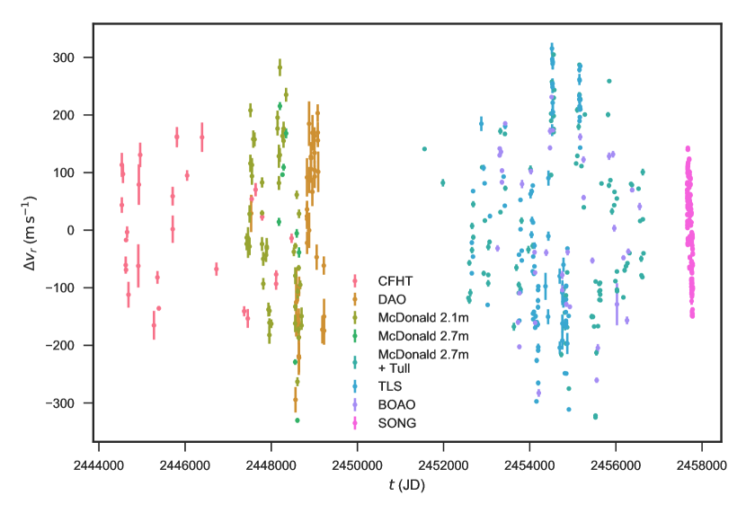
Figure 1: All archival and new radial velocities used for inference in this work. The site and instrument for each data set is indicated in the legend (see text for a full description).

Figure 2: Posterior for $\nu_{\rm max}$ from the complete, combined RV data set described in this paper (blue), the archival data from Hatzes et al. (2015) (green), and the SONG data described in Section 4.2 (red). The inference on the archival data is consistent with the independent inference on the SONG data set alone.

4.2 SONG Observations

In order to confirm the oscillations detected in the archival data, we used the Hertzsprung SONG telescope (Grundahl et al., 2017) to conduct high time cadence follow-up observations. These were carried out in the highest resolution mode ($R\approx 110000$) with an integration time of 30 s, between 2016 September 27 and 2017 January 12. During this time we attempted to obtain at least one visit per available night, for a total of 254 epochs over the campaign. The spectra were extracted using the SONG pipeline (see Grundahl et al., 2017). SONG employs an iodine cell for precise wavelength calibration and the velocities were determined using the iSONG software following the same procedures as described in Grundahl et al. (2017). The typical velocity precision per visit is 2.5$\,\rm m\,s^{-1}$ allowing us to easily detect the oscillations which display a peak-to-peak amplitude of $\approx\,170\,\rm m\,s^{-1}$. Figure 3 displays the radial velocities obtained—oscillations are easily visible as well as a long-term trend, due to the planetary companion. From this data set alone we also find evidence for a low-quality ($Q=3.1^{+1.2}_{-0.8}{}$) oscillatory mode with $\nu_{\mathrm{max}}=2.33^{+0.13}_{-0.14}{}\,\mu\mathrm{Hz}$ which is consistent with the inference from the archival data. This posterior is shown in Figure 2.

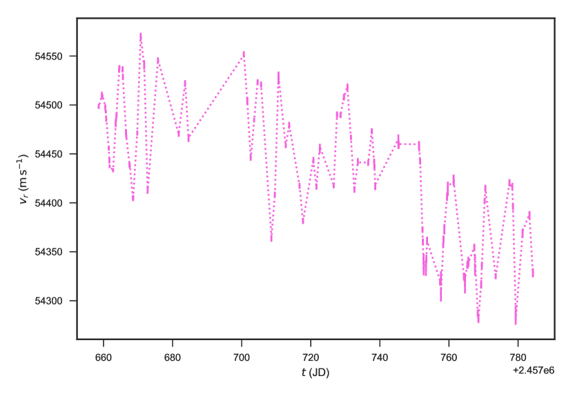
Figure 3: New radial velocities of Aldebaran obtained by the Hertzsprung SONG Telescope. Clear oscillations can be seen, plus a trend representing part of the planetary orbit.

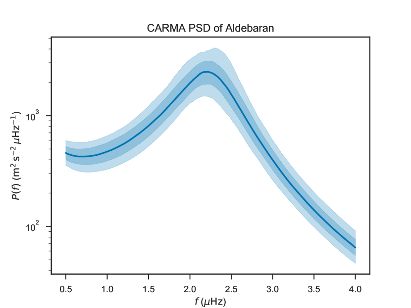
Figure 4: CARMA-derived power spectral density from archival and SONG RV observations of Aldebaran, showing the clear peak at around 2 $\mu$Hz. The dark and light shaded regions represent $1\,\sigma$ and $2\,\sigma$ posterior probability contours.

4.3 K2 Observations

In order to verify the results of the novel analysis presented above, we sought to obtain an independent detection of the oscillations of Aldebaran and compare the frequencies determined with the two methods. Aldebaran was observed with K2 (Howell et al., 2014), a two-wheeled revival of the Kepler Mission (Borucki et al., 2010), under Guest Observer Program 130471 in Campaign 13, from 2017 March 8 to 2017 May 27. Aldebaran and similar high-luminosity K giants are well known to show photometric variability due to solar-like oscillations (Bedding, 2000), and hence the continuous, high-precision K2 light curves allow an independent confirmation of our CARMA results.

As Aldebaran is extremely bright, it saturates the Kepler detector and it is therefore not possible to use standard photometry pipelines to extract a K2 lightcurve. We instead use halo photometry (White et al., 2017), whereby unsaturated pixels from the outer part of the large and complicated halo of scattered light around bright stars are used to reconstruct a light curve as a weighted linear combination of individual pixel-level time series, as described in Appendix B.

Figure 5 shows the light curve and power spectrum of the K2 observations of Aldebaran. We detect clear variability on an average timescale of $\sim$ 5 days, consistent with the expected timescale for solar-like oscillations for a high-luminosity red giant. To measure global asteroseismic parameters we model the background variability in the Fourier domain using the methodology described in Huber et al. (2009), yielding a frequency of maximum power of $\mbox{$\nu_{\rm max}$}=2.2\pm 0.25\,\mbox{$\mu$Hz}$ and amplitude per radial mode of $1850\pm 500$ ppm. Due to the limited frequency resolution of the 70-day K2 time series we were unable to measure the large frequency separation $\Delta\nu$, which is expected to be $\approx$ 0.5$\mu$Hz.

Using the k2ps planet-search code (Parviainen et al., 2016; Pope et al., 2016a) to examine this light curve, we search for transits across a wide range of periods, and find no evidence either of short-period planetary transits or an eclipsing stellar companion.

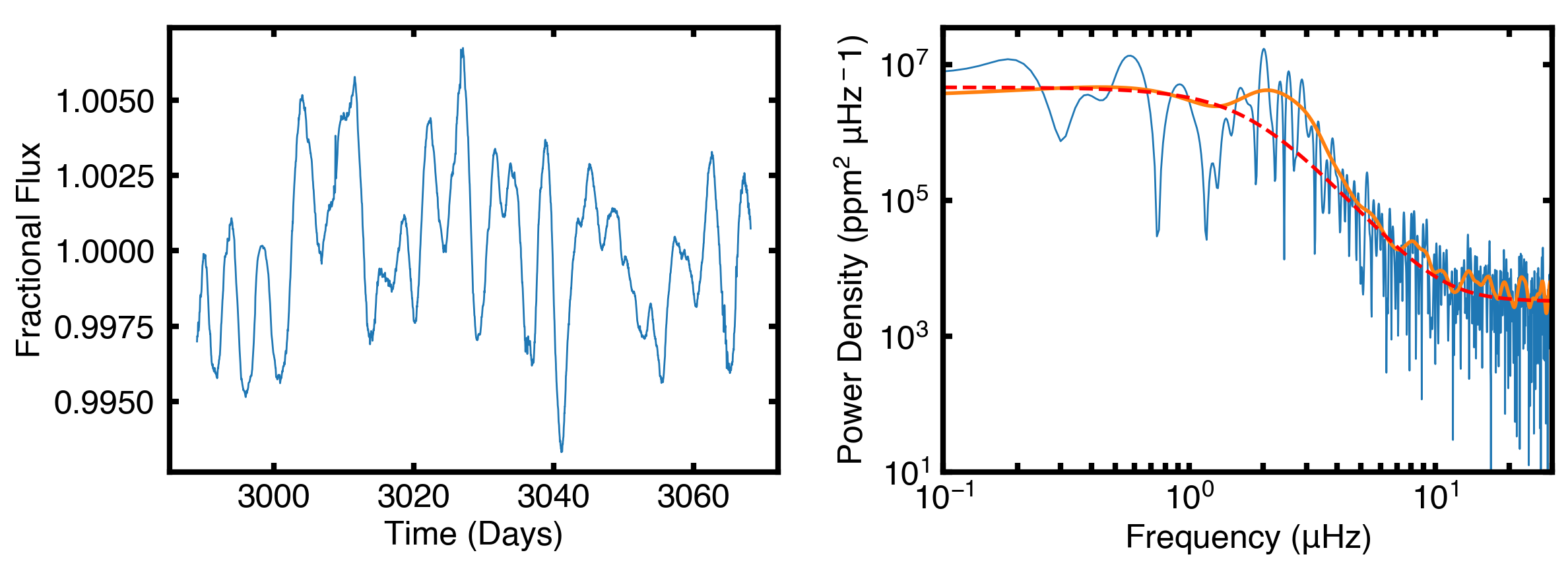
Figure 5: K2 lightcurve (left) and power spectrum (right) of Aldebaran. The red dashed line shows the background model, and the orange line is a heavily smoothed version of the power spectrum used to measure the frequency of maximum power.

4.4 Planetary and Stellar Parameters

By jointly fitting a Keplerian for the planet with a CARMA model for the stellar oscillations to the combined archival and SONG data sets (Figure 1), we obtain a precise estimate of both $\nu_{\rm max}$ and the planetary orbital parameters. The planetary orbital parameters we obtain are similar to Hatzes et al. (2015), but with larger uncertainty that is likely due to our more-flexible and correlated model for the stellar component of the RV signal: period $P=629.0^{+1.7}_{-2.1}{}\,\mathrm{d}$, eccentricity $e=0.17\pm 0.07{}$; and radial velocity semi-amplitude $K=127^{+15}_{-14}{}\,\mathrm{m}\,\mathrm{s}^{-1}$.

The stellar oscillations are best fit with a single, low-quality ($Q=2.8^{+0.6}_{-0.5}{}$) oscillatory mode with $\mbox{$\nu_{\rm max}$}=2.24^{+0.09}_{-0.08}$ $\mu$Hz. We find no improvement in the marginal likelihood (evidence) or other model-selection information criteria (Gelman et al., 2013) from models with additional oscillatory modes, so we conclude that the large spacing $\Delta\nu$ is not observable in this data set.

We have used the additional constraint of $\nu_{\rm max}$ determined from this analysis to update the stellar properties of Aldebaran. The details of the stellar modelling are presented in Appendix C. We have considered the impact of our additional $\nu_{\rm max}$ constraint and run our analysis for different sets of spectroscopic estimates. For final values we adopt the Sheffield et al. (2012) spectroscopic solution as being ‘middle of the road’ estimates. For the analysis without constraint on $\nu_{\rm max}$ we find estimates of the stellar properties as $M=1.27^{+0.24}_{-0.20}\,\mathrm{M_{\odot}}$ and age $4.9^{+3.6}_{-2.0}\,\rm Gyr$. With the inclusion of $\nu_{\rm max}$ we find $M=1.16\,\pm\,{0.07}\,\mathrm{M_{\odot}}$ and age $6.4^{+1.4}_{-1.1}\,\rm Gyr$. It is clear that the addition of $\nu_{\rm max}$ provides substantially more precise estimates of mass and age. With this stellar mass, the radial velocity signal translates to an inclination-dependent planetary mass of $M\,\sin\,{i}=5.8\pm 0.7~{}M_{J}$ (Torres et al., 2008, Equation 1), a massive giant planet; for sufficiently high inclinations ($\gtrsim 45^{\circ}$), the mass of Aldebaran b may exceed $13~{}M_{J}$, making it a possible low-mass brown dwarf candidate. A recent study by Hatzes et al. (2018) has cast doubt on the validity of the detection of the massive planet $\gamma$ Draconis b, and by extension similar planets around similar K giants such as Aldebaran. We remain convinced that the $\gamma$ Draconis problem is not an issue in this case, and Aldebaran b is a bona fide planet, for reasons outlined in Appendix D.

With the determination of the stellar mass it is possible to infer the parameters Aldebaran had while it was on the main sequence. We conduct a Monte Carlo simulation, drawing masses randomly from a Gaussian distribution $M\sim\mathcal{N}(1.16,0.07)$ and metallicities $[\text{Fe}/\text{H}]\sim\mathcal{N}(-0.15,0.2)$ (Decin et al., 2003) to predict the luminosity of the main-sequence progenitor, and the semi-major axis of the planet’s orbit. Using the Mesa Isochrones and Stellar Tracks (MIST: Dotter, 2016; Choi et al., 2016) models, we compute the evolution of the luminosity $L$ of the star along the main sequence; $L$ evolves from $2.0\pm 0.7$ $\mathrm{L}_{\odot}$ at 0.5 Gyr to $3.5\pm 2.3$ $\mathrm{L}_{\odot}$ at 4.5 Gyr. We note that this implies that the planet at a semi-major axis of $1.50\,\pm\,0.03$ AU would have been subject to an insolation comparable to that of the Earth, evolving from 0.5 Gyr to 4.5 Gyr from $0.86\,\pm\,0.27$ to $1.55\,\pm\,1.0$ times that of the Earth today (Figure 6). Subject as well as this to the great uncertainties of the planet’s orbital evolution and albedo, Aldebaran b and any of its moons (or its S-type planets if it is a brown dwarf) may well have hosted temperate environments for some of their history, now long-since destroyed by their star’s evolution away from the main sequence.

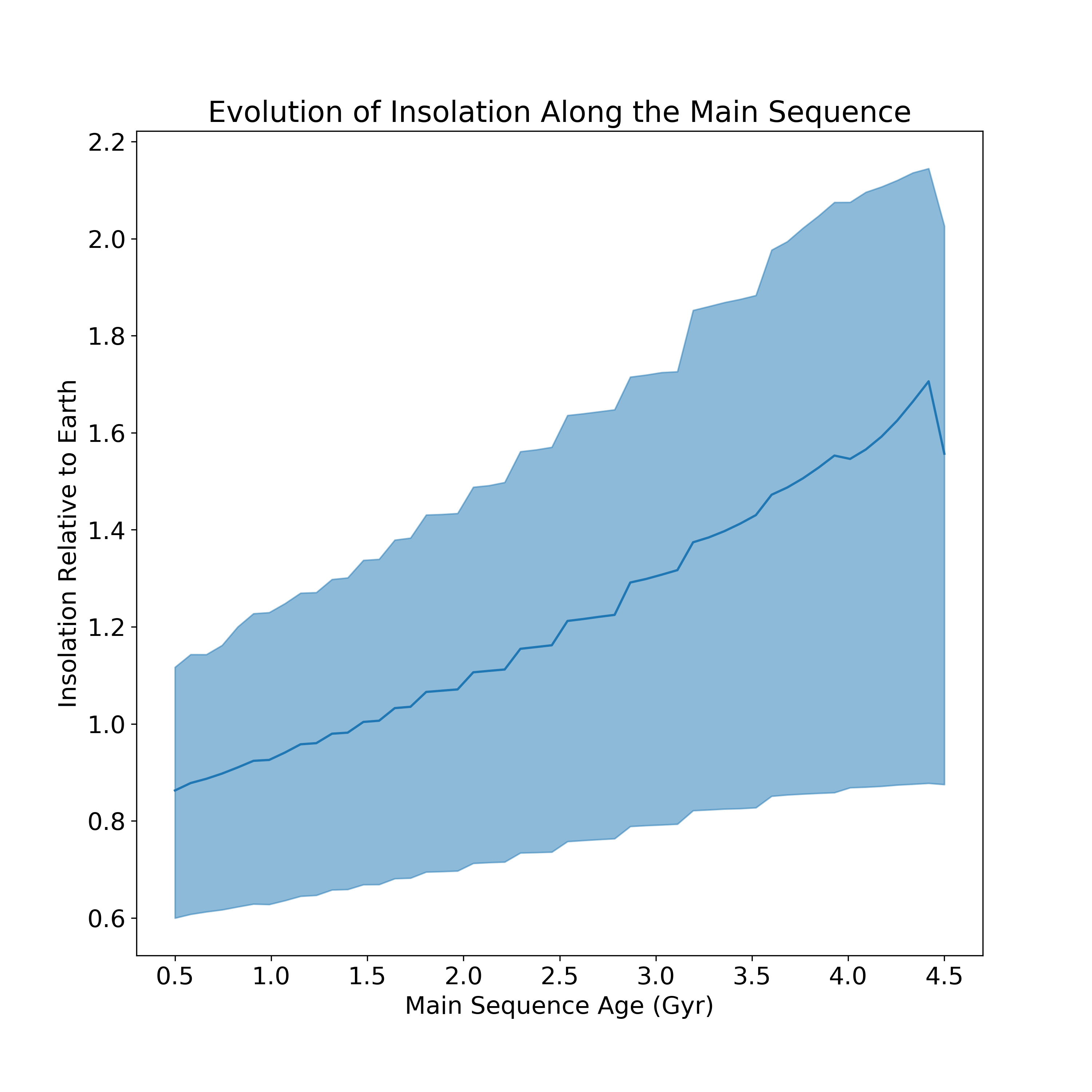
Figure 6: Evolution of the insolation of Aldebaran b relative to the incident sunlight on Earth, as a function of the age of Aldebaran on the main sequence. The solid line is the mean of simulations, and the shaded region represents $1\,\sigma$ equivalent deviations. It is likely that Aldebaran b spent some time on the main sequence with an equilibrium temperature similar to Earth.

5 Conclusions

Using sophisticated time-domain CARMA models for the stellar activity in Aldebaran, we have confirmed the previously-suspected planet and additionally detected acoustic oscillations that permit a mass determination with a precision of $\sim 6\%$. We have confirmed both of these results with new ground-based observations, and space-based photometry with K2.

From this pilot study with Aldebaran, we have shown that with limited quantities of data of limited quality, we can nevertheless do asteroseismology from the ground and obtain very precise estimates of stellar parameters. Furthermore, improvements in the algorithm may also permit the detection of not only $\nu_{\rm max}$ but also $\Delta\nu$ from similar measurements, permitting more sophisticated asteroseismic analysis. Sufficient radial velocity data either already exist, or are trivial to obtain, in order to do this for essentially all bright giants; while for asteroseismology of solar-like stars, these new methods will allow significantly relaxed observing requirements. One rich archive is the series of observations with the Hamilton Échelle Spectrograph at Lick Observatory, studying 373 G and K giants (e.g. Frink et al., 2001; Hekker et al., 2006; Ortiz et al., 2016). The method may also be useful in detecting rotational or other periodic variability in the LCES HIRES/Keck Precision Radial Velocity Exoplanet Survey (Butler et al., 2017) of 1,624 FGKM dwarfs, although the time sampling is by design too coarse to detect $p$-mode oscillations in these stars. Furthermore, CARMA models and related methods will enhance deep, all-sky, sparse photometric surveys: an immediate future test of this will be from Hipparcos; while only 58 epochs of photometry are available for Aldebaran, at a sampling we find to be insufficient for our purposes, stars at higher latitudes may often have 150–200 epochs and more even sampling (van Leeuwen, 1997), and the 14 bright K giants in Hipparcos noted by Bedding (2000) are an ideal first test case. This can naturally be extended to Gaia in space (Gaia Collaboration et al., 2016), or LSST from the ground (Angel et al., 2000; Tyson & Angel, 2001; LSST Science Collaboration et al., 2009), from which many thousands of new asteroseismic determinations will be possible. In future RV surveys, it may be possible to beat the Sato et al. (2005) $\sim 30$ m/s RV precision limit for red giants by taking many closely spaced observations and modelling-out the effects of stellar oscillations: this will allow us to dig deeper into this intrinsic stellar noise to detect less-massive planets around these stars.

Appendix A CARMA Models

A CARMA process corresponds to the solution, $y(t)$, of the stochastic ODE

$$\prod_{i=1}^{p}\left[\frac{\mathrm{d}}{\mathrm{d}t}-r_{i}\right]y(t)=\prod_{j=1}^{q}\left[\frac{\mathrm{d}}{\mathrm{d}t}-b_{i}\right]\eta(t),$$ (A1)

where $p,q\in\mathbb{Z}$, $p>q\geq 0$ define the order of the process; $r_{i}\in\mathbb{C}$, $\Re r_{i}<0$ are the roots of the characteristic equation of the ODE; $b_{j}\in\mathbb{C}$, $\Re b_{j}<0$ are corresponding roots of the inverse process; and $\eta(t)$ is a white-noise GP with $\left\langle\eta(t)\right\rangle=0$ and $\left\langle\eta(t)\eta(t^{\prime})\right\rangle=\sigma^{2}\delta\left(t-t^{\prime}\right)$. The constraint that $\Re r_{i}<0$ and $\Re b_{j}<0$ ensures that the linear operator defining the process and its inverse are invertable. Under the assumption that the solution, $y(t)$, is real, roots $r_{i}$ and $b_{j}$ must either be real or occur in complex conjugate pairs. The power spectrum of the process is

$$P_{y}(f)=\sigma^{2}\left|\frac{\prod_{j=1}^{q}\left[2\pi if-b_{j}\right]}{\prod_{i=1}^{p}\left[2\pi if-r_{i}\right]}\right|^{2}.$$ (A2)

The power spectrum is a rational function of frequency with poles at $2\pi if=r_{i}$ and zeros at $2\pi if=b_{i}$; because of the invertable constraints, these poles and zeros all occur when $\Im f\neq 0$. The autocorrelation function corresponding to the power spectrum in Eq. (A2) is

$$\rho_{y}(\tau)=\left\langle y\left(t\right)y\left(t+\tau\right)\right\rangle=\sum_{i=1}^{p}A_{i}^{2}e^{r_{i}\tau},$$ (A3)

where the RMS amplitudes of the $p$ different modes, $A_{i}$, are functions of $\sigma$ and the values of the roots $r_{i}$ and $b_{j}$. If $q=p-1$, then the $A_{i}$ are independent, while if $q<p-1$ then there are interdependencies among the $A_{i}$. From either the power spectrum in Eq. (A2) or the autocorrelation function in Eq. (A3), it is apparent that a real root $r_{i}$ represents an exponentially-decaying mode with $r_{i}$ the rate constant, while a complex conjugate pair of $r_{i}$ represent an oscillatory mode with decay rate $\Re r_{i}$ and angular frequency $\left|\Im r_{i}\right|$. Oscillatory modes can also be described by their frequency $f$ and quality factor $Q$ via $r=f/(2Q)\pm 2\pi if$. Decaying modes generate a damped random walk, also known as a Ornstein-Uhlenbeck process. More discussion of CARMA processes, including formulae for $A_{i}$ in terms of $\sigma$, $r_{i}$, and $b_{j}$, can be found in Kelly et al. (2014) and references therein.

Our preferred model for the data uses one decaying mode and one oscillatory mode in the CARMA process to capture the un-resolved superposition of many asteroseismic modes (see Section 4.4); we have fit models with more than one mode of each type, but find no improvement in model-selection criteria from the expanded parameter space. The priors we impose in all cases on the parameters of the CARMA model, planetary RV signal, and instrumental and site effects are given in Table 1. A draw from the posterior for our canonical model in shown in data space in Figure 7.

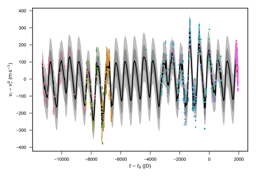
Figure 7: A posterior draw from our model plotted with the observed radial velocities. Each site’s radial velocity has been shifted by the model’s site-specific RV offset and errorbars have been scaled by the model’s site-specific errorbar scaling. Data colors are as in Figure 1. The black line gives the sum of the model’s Keplerian component and the mean of the inferred stochastic component; the dark and light bands give the 1- and 2-sigma uncertainty in the inferred stochastic component. Between observations, the uncertainty in the stochastic component increases; it reduces near observations, as each observation provides some information about the stellar noise that propogates to nearby times because of the temporal correlation in the noise. Stellar oscillations are apparent in the short-timescale wiggles in the stochastic component between nearby observations; there is also a significant long-period correlated component (represented in our model by an exponentially-decaying eigenmode).

The Kalman filter implementation of the CARMA likelihood is not unique. Foreman-Mackey et al. (2017) show how a dimensional expansion can be used to reduce the standard GP covariance matrix for this same process, with autocorrelation given by Eq. (A3) under observations at times $t_{k}$, to a banded form that can then be Cholesky-decomposed in the standard GP likelihood function in $\mathcal{O}\left(n\right)$ time. These ‘celerite’ models are formally equivalent to a Kalman CARMA model with $q=p-1$ and differ only in their computational implementation.

Table 1: The parameters in our model Eq. (4) and their priors. Site and instrument combinations are indexed by $j$. Modes in the stochastic process are indexed by $k\in[1,p]$ and are either real (parameterised by a rate parameter $r_{k}$) or complex (parameterised by a frequency $f_{k}$ and quality factor $Q_{k}$).

Parameter	Prior	Description
Site/Instrument RV Offset and Uncertainty Scaling
$\mu_{j}$	$N\left[\left\langle y_{j}\right\rangle,10\sigma_{y_{j}}\right]\left(\mu_{j}\right)\tablenotemark{a}$	The site/instrument RV offset.
$\nu_{j}$	$1/\nu_{j},\quad\nu_{j}\in[1/2,2]$	The site/instrument uncertainty scale factor.
Keplerian Parameters
$K$	$1/K,\quad K\in\left[\min_{j}\sigma_{y_{j}}/100,\max_{j}10\sigma_{y_{j}}\right]$	RV semi-amplitude.
$P$	$1/P,\quad P\in[600,700]\,\mathrm{d}$	Keplerian period
$e$	$2e,\quad 0\leq e<1$	Keplerian eccentricity
$\omega$	$\mathrm{const},\quad 0\leq\omega<2\pi$	Longitude of pericentre
$\chi$	$\mathrm{const},\quad 0\leq\chi<1$	Pericentre passage is at $t=\chi P$
CARMA Parameters
$A_{k}$	$1/A_{k},\quad A_{k}\in\left[\min_{j}\sigma_{y_{j}}/100,\max_{j}10\sigma_{y_{j}}\right]$	RMS amplitude of stochastic mode
$r_{k}$	$1/r_{k},\quad\Re r_{k}\in\left[1/(2T),0.05\,\mu\mathrm{Hz}\right],\Im r_{k}=0$	The damping rates for real modes
$f_{k}$	$1/f_{k},\quad f_{k}\in\left[0.1,10\right]\mu\mathrm{Hz}$	The frequency of oscillatory modes
$Q_{k}$	$1/Q_{k},\quad Q_{k}\in\left[1,1000\right]$	The quality factor of oscillatory modes

Appendix B Halo Photometry

The Kepler Space Telescope (Borucki et al., 2010) suffered a critical reaction wheel failure in May 2013, which made it impossible to maintain a stable pointing and therefore continue its nominal mission. It was revived as K2 (Howell et al., 2014), balanced by orienting perpendicular to the Sun. This requires that K2 observes fields in the Ecliptic in $\sim 80$ d Campaigns; Aldebaran was observed in Campaign 13.

The Kepler detector saturates for stars brighter than the $\sim 11^{\text{th}}$ magnitude. Nevertheless, the excess flux deposited in a saturated pixel spills conservatively up and down the pixel column, such that it is possible to sum this ‘bleed column’ for bright stars and still obtain precise photometry, such as was done for the brightest star in the nominal Kepler mission, $\theta$ Cyg ($V=4.48$; Guzik et al., 2011; White et al., 2013; Guzik et al., 2016). There are two main reasons why this is not possible for all bright stars in general. First, because the on-board data storage and downlink bandwidth from Kepler are limited, it is often not desirable to store and download the large number of pixels that are required for such bright stars. Second, if the bleed column for a sufficiently bright star reaches the edge of the chip, flux spills over and is not conserved, imposing a hard brightness limit that depends on the distance to the detector edge. Collateral ‘smear’ data, which are collected to help calibrate the photometric bias from stars sharing the same column as a target, can be used to reconstruct light curves for un-downloaded bright stars and thereby avoid bandwidth constraints (Pope et al., 2016b), but these data are still rendered unusable if the bleed column falls off the edge of the chip and contaminates the smear rows.

Bright stars have a wide, complicated, position-dependent point spread function (PSF) arising from diffraction and scattering from secondary and higher-order reflections inside the instrument, with the result that they may contaminate thousands of nearby pixels with significant flux. We can therefore use this ‘halo’ of unsaturated pixels for photometry. The brightness of this halo varies in the same way as that of the primary star, and we therefore obtain data in a region of 20 pixel radius around the mean position of Aldebaran, and discard saturated pixels. In this paper we proceed as in White et al. (2017), in which the method was demonstrated on the seven bright Pleiades, with only minor changes.

The flux $f_{i}$ at each cadence $i$ is constructed as a weighted sum of pixel values $p_{ij}$:

$$f_{i}=\sum_{j=1}^{M}w_{j}p_{ij}.$$ (B1)

We choose the weights $w_{j}$ such that they lie between 0 and 1, add to unity, and minimize the Total Variation (TV) of the weighted light curve. In the continuous case, $n$-th order TV is defined as the integral of the absolute value of the $n$-th derivative of a function; in the discrete case, replacing the derivative with finite differences, first-order TV becomes

$$\text{TV}=\dfrac{\sum_{i=1}^{N}|{f}_{i}-{f}_{i-1}|}{\sum_{j=1}^{N}{f}_{j}}$$ (B2)

and likewise second-order TV the equivalent expression in second-order finite differences. The efficacy of this method was recently confirmed by Kallinger & Weiss (2017), comparing BRITE-Constellation observations of Atlas to K2 halo photometry and finding excellent agreement in the frequency and amplitude of the reported oscillations.

In an improvement since White et al. (2017), we use the autograd library (Maclaurin et al., 2015) to calculate analytic derivatives for the TV objective function, which reduces the computational time for a single halo light curve on a commercial laptop from tens of minutes to a few seconds.

As a final step to reduce residual uncorrected systematics, we apply the k2sc (Aigrain et al., 2016) GP-based systematics correction code to the initial halo light curve, but the effect of this in the present case for Aldebaran is minimal. There is somewhat higher than usual residual noise at harmonics of $46\,\mu\mathrm{Hz}$ ($4\,\mathrm{d}^{-1}$, the satellite thruster firing frequency), but this is nevertheless very small in comparison to the signal from Aldebaran, and may be ascribed to the large fraction of the pixel mask occupied by the bleed column from this extremely bright star.

Appendix C Stellar Modelling

C.1 Stellar Models

We used our determination of $\nu_{\rm max}$ and several combinations of the asteroseismic and spectroscopic parameters, along with luminosity, to estimate the fundamental stellar parameters, via fitting to stellar models. We used MESA models (Paxton et al., 2011, 2013) in conjunction with the Bayesian code PARAM (da Silva et al., 2006; Rodrigues et al., 2017). A summary of our selected “benchmark” options is as follows;

• Heavy element partitioning from Grevesse & Noels (1993).

• OPAL equation of state (Rogers & Nayfonov, 2002) along with OPAL opacities (Iglesias & Rogers, 1996), with complementary values at low temperatures from Ferguson et al. (2005).

• Nuclear reaction rates from NACRE (Angulo et al., 1999).

• The atmosphere model according to Krishna Swamy (1966).

• The mixing length theory to describe convection (we adopt a solar-calibrated parameter $\alpha_{\textrm{MLT}}=1.9657$).

• Convective overshooting on the main sequence is set to $\alpha_{\textrm{ov}}=0.2H_{p}$, with $H_{p}$ the pressure scale height at the border of the convective core. Overshooting was applied according to the Maeder (1975) step function scheme.

• No rotational mixing or diffusion is included.

We do not need to correct for the line-of-sight Doppler shift at the frequency precision available in our data (Davies et al., 2014).

C.2 Additional modelling inputs

In addition to the asteroseismic parameters, spectroscopically-determined temperature and metallicity values are needed. There exist multiple literature values for Aldebaran. We chose to compare a range of literature values to investigate what uncertainty these systematically-differing models produce in inferred stellar properties.

To ensure the values are self-consistent, when a literature value was chosen for temperature, we took the stellar metallicity from the same source i.e. matched pairs of temperature and metallicity. The final constraint is the stellar luminosity, which may be estimated as follows (e.g. see Pijpers 2003):

$$\log_{10}\frac{L}{L_{\odot}}=4.0+0.4M_{{\textrm{bol}},\odot}-2.0\log_{10}{\pi[{\textrm{mas}]}}-0.4(V-A_{V}+BC(V)).$$ (C1)

The solar bolometric magnitude $M_{\textrm{bol},\odot}=4.73$ is taken from Torres (2010), from which we also take the polynomial expression for the bolometric correction $BC(V)$. We assume extinction $A_{V}$ to be zero.

The final constraint available for Aldebaran is the angular diameter of the star as measured by long baseline interferometry and lunar occultations ($20.58\pm 0.03$ mas; Richichi & Roccatagliata, 2005; Beavers & Eitter, 1979; Brown et al., 1979; Panek & Leap, 1980), combined with the Hipparcos parallax of $19.96\pm 0.38$ pc to produce a physical radius constraint of $R_{\textrm{int}}=44.2\pm 0.9\textrm{R}_{\odot}$.

Table 2: Spectroscopic stellar parameters from each literature source, along with calculated luminosity. All temperature uncertainties assumed to be 50K, 0.2 dex in $\log{g}$, and 0.1 dex in [FeH]. For the two Sheffield et al. (2012) results, the reason for discrepancy between the two sets of metallicity results is not discussed.

Spectrosocpy Source	$T_{\textrm{eff}}$ (K)	$\log{g}$ (dex)	[FeH] (dex)	Luminosity (L⊙)
Sheffield et al. (2012)a	3900	1.3	0.17	480
Sheffield et al. (2012)b	3900	1.3	0.05	480
Prugniel et al. (2011)	3870	1.66	-0.04	507
Massarotti et al. (2008)	3936	1	-0.34	456
Frasca et al. (2009)	3850	0.55	-0.1	526

As Table 2 shows, the spectroscopic parameters of Aldebaran are somewhat unclear, particularly $\log{g}$ and [FeH], which may have an impact on the recovered stellar properties when fitting to models. To explore what impact each parameter is having on the final stellar properties, multiple PARAM runs were performed, using different constraints. Two constraints potentially in tension were $\nu_{\textrm{max}}$ and the spectroscopically-determined $\log{g}$. $\nu_{\textrm{max}}$ has been shown to scale with the stellar $\log{g}$ (Kjeldsen & Bedding, 1995; Belkacem et al., 2011),

$$\frac{\nu_{\textrm{max}}}{\nu_{\textrm{max},\odot}}=\frac{\log{g}}{\log{g},\odot}\left(\frac{T_{\textrm{eff}}}{T_{\textrm{eff},\odot}}\right)^{-1/2}.$$ (C2)

Using Eq C2 with the values in Table 2 predicts $\nu_{\textrm{max}}$ in the range $0.5-6\mu$Hz. Reversing the equation to produce a predicted $\log{g}$ from the observed $\nu_{\textrm{max,obs}}=2.23\pm 0.1\mu$Hz results in a predicted $\log{g}\sim 1.2$ dex, using an assumed temperature of 3900K. The solar calibration values used here are $\log g_{\odot}/\left(\mathrm{m}\,\mathrm{s}^{-1}\right)=2.44\,\mathrm{dex}$, $\nu_{\textrm{max},\odot}=3150\,\mu$Hz and $T_{\textrm{eff},\odot}=5777\,$K.

Table 3 shows the results, for all modelling variations, both different inputs and different constraints. It shows that results with the addition of $\nu_{\textrm{max}}$ as a constraint exhibit in general smaller uncertainties, with or without the addition of $\log{g}$ as a constraint.

Recovering the mass without the use of asteroseismic constraints produces considerable scatter on the results ($0.96-1.5\textrm{M}_{\odot}$), whilst the use of asteroseismology brings the mass estimates into closer agreement with one another, with the exception of the very low metallicity solution of Massarotti et al. (2008). Any systematic offset between asteroseismic masses and spectroscopic masses is sensitive to chosen reference mass, in agreement with North et al. (2017).

We have also investigated running PARAM and relaxing one or more constraints: between runs with and without the luminosity constraint, the average absolute mass offset between the two sets of results was $<0.04\textrm{M}_{\odot}$ if we also ignore the $\nu_{\textrm{max}}$ constraint, and $<0.02\textrm{M}_{\odot}$ including the $\nu_{\textrm{max}}$.

Table 3: Recovered stellar properties from PARAM using various constraints. Uncertainties quoted are the 68% credible interval.

Spectroscopy Source	Mass ($\textrm{M}_{\odot}$)	Radius ($\textrm{R}_{\odot}$)	Age (Gyr)
$\nu_{\textrm{max}}$, $\log{g}$, $T_{\textrm{eff}}$, $R_{\textrm{int}}$, L and [FeH].
Sheffield et al. (2012)a	$1.17^{+0.07}_{-0.07}$	$43.9^{+0.9}_{-0.9}$	$6.5^{+1.4}_{-1.1}$
Sheffield et al. (2012)b	$1.17^{+0.07}_{-0.07}$	$43.8^{+0.8}_{-0.9}$	$6.4^{+1.4}_{-1.1}$
Prugniel et al. (2011)	$1.17^{+0.07}_{-0.07}$	$43.9^{+0.9}_{-0.9}$	$6.2^{+1.4}_{-1.1}$
Massarotti et al. (2008)	$1.13^{+0.07}_{-0.07}$	$43.5^{+0.9}_{-0.9}$	$6.0^{+1.4}_{-1.1}$
Frasca et al. (2009)	$1.02^{+0.04}_{-0.04}$	$44.0^{+0.8}_{-0.8}$	$10.3^{+1.5}_{-1.4}$
$\log{g}$, $T_{\textrm{eff}}$, $R_{\textrm{int}}$, L and [FeH].
Sheffield et al. (2012)a	$1.43^{+0.26}_{-0.24}$	$43.8^{+0.9}_{-0.9}$	$3.5^{+2.7}_{-1.4}$
Sheffield et al. (2012)b	$1.27^{+0.24}_{-0.2}$	$43.8^{+0.9}_{-0.9}$	$4.9^{+3.6}_{-2.0}$
Prugniel et al. (2011)	$1.25^{+0.22}_{-0.19}$	$43.8^{+0.9}_{-0.9}$	$5.0^{+3.5}_{-2.0}$
Massarotti et al. (2008)	$0.95^{+0.11}_{-0.05}$	$43.8^{+0.9}_{-0.9}$	$10.2^{+2.4}_{-3.1}$
Frasca et al. (2009)	$0.96^{+0.04}_{-0.04}$	$44.4^{+0.8}_{-0.8}$	$11.6^{+1.4}_{-1.8}$
$\nu_{\textrm{max}}$, $T_{\textrm{eff}}$, $R_{\textrm{int}}$, L and [FeH].
Sheffield et al. (2012)a	$1.17^{+0.07}_{-0.07}$	$43.9^{+0.9}_{-0.9}$	$6.5^{+1.4}_{-1.1}$
Sheffield et al. (2012)b	$1.16^{+0.07}_{-0.07}$	$43.8^{+0.8}_{-0.9}$	$6.4^{+1.4}_{-1.1}$
Prugniel et al. (2011)	$1.16^{+0.07}_{-0.07}$	$43.9^{+0.9}_{-0.9}$	$6.4^{+1.5}_{-1.2}$
Massarotti et al. (2008)	$1.13^{+0.07}_{-0.07}$	$43.5^{+0.9}_{-0.9}$	$5.9^{+1.4}_{-1.0}$
Frasca et al. (2009)	$1.15^{+0.07}_{-0.07}$	$43.9^{+0.9}_{-0.8}$	$6.5^{+1.5}_{-1.2}$

Appendix D The $\gamma$ Draconis Problem is Not a Problem

$\gamma$ Draconis (also known as Eltanin, or $\gamma$ Dra) is a second-magnitude K5III giant which had been observed by Hatzes & Cochran (1993) as part of the same campaign that led to the discovery of Aldebaran b and Pollux b. Hatzes et al. (2018) have recently shown that the 702 d period RV variations of the putative Eltanin b disappeared from 2011-2013, returning in 2014 with a different amplitude and phase. They ascribe this to a previously-unidentified kind of stellar variability, and warn that “Given that the periods found in $\alpha$ Tau [Aldebaran] are comparable to those in $\gamma$ Dra and both stars are evolved with large radii, a closer scrutiny of the RV variability of $\alpha$ Tau is warranted.”

For several reasons we are not convinced that this poses an issue for Aldebaran or for K giant RV planets more generally. Hatzes et al. (2018) suggest that the new type of stellar variability may be oscillatory convective modes, but both Aldebaran and Eltanin have much lower luminosities and longer periods than would seem to be allowed by the period-luminosity relation predicted for these otherwise unobserved modes (Saio et al., 2015; Hatzes et al., 2018, Figure 9). If these are identified with the long secondary periods (LSPs) observed in some bright red giants ($L\approx 1000\,\mbox{$\mathrm{L}_{\odot}$}$), then Aldebaran and Eltanin are both too faint, and lack the mid-IR excess typical of LSP stars (Wood & Nicholls, 2009). It would also be surprising if the shape of the RV curve could reproduce the harmonic structure of an eccentric Keplerian such as in Aldebaran b ($e=0.17\pm 0.07{}$), let alone the much higher eccentricities observed in other giants (e.g. $\iota$ Dra b, $e=0.7$: Frink et al., 2002).

It would be a cruel conspiracy of nature if red giants support a type of oscillation which is common and closely resembles a planetary signal. We believe this cannot be the case: the populations of planets around subgiants and giants evolved from intermediate mass stars are similar (Jones et al., 2014), as expected if subgiants evolve into giants and retain their planetary systems, and with very different stellar structures subgiants and giants are unlikely to share modes of long-period pulsation. The similarity of distributions of systems hosted by subgiant and giants could not be reproduced if a large fraction of the giants’ planets were false positives. Moreover giant planets are expected to be common around intermediate-mass stars (Kennedy & Kenyon, 2008), and some are definitely known to be bona fide planets because they transit their star (e.g. Lillo-Box et al., 2014; Ortiz et al., 2015; Grunblatt et al., 2016, 2017).

We therefore believe that either Eltanin b is not a false positive, or if it is, that it is not a common type of false positive, and is unlikely to affect our certainty that Aldebaran b is real. Hatzes et al. (2018) offer an alternative to the pulsation hypothesis, namely beating between the stellar rotation and the planetary signal; this does not seem implausible.

References

- Aigrain et al. (2016) Aigrain, S., Parviainen, H., & Pope, B. J. S. 2016, MNRAS, 459, 2408
- Angel et al. (2000) Angel, R., Lesser, M., Sarlot, R., & Dunham, E. 2000, in Astronomical Society of the Pacific Conference Series, Vol. 195, Imaging the Universe in Three Dimensions, ed. W. van Breugel & J. Bland-Hawthorn, 81
- Angulo et al. (1999) Angulo, C., Arnould, M., Rayet, M., et al. 1999, Nuclear Physics A, 656, 3
- Astropy Collaboration et al. (2013) Astropy Collaboration, Robitaille, T. P., Tollerud, E. J., et al. 2013, A&A, 558, A33
- Beavers & Eitter (1979) Beavers, W. I., & Eitter, J. 1979, ApJ, 228, L111
- Bedding (2000) Bedding, T. R. 2000, in The Third MONS Workshop: Science Preparation and Target Selection, ed. T. Teixeira & T. Bedding, 97
- Belkacem et al. (2011) Belkacem, K., Goupil, M. J., Dupret, M. A., et al. 2011, A&A, 530, A142
- Bezanson et al. (2017) Bezanson, J., Edelman, A., Karpinski, S., & Shah, V. B. 2017, SIAM Review, 59, 65. https://doi.org/10.1137/141000671
- Borucki et al. (2010) Borucki, W. J., Koch, D., Basri, G., et al. 2010, Science, 327, 977
- Brewer & Stello (2009) Brewer, B. J., & Stello, D. 2009, MNRAS, 395, 2226
- Brown et al. (1979) Brown, A., Bunclark, P. S., Stapleton, J. R., & Stewart, G. C. 1979, MNRAS, 187, 753
- Butler et al. (2017) Butler, R. P., Vogt, S. S., Laughlin, G., et al. 2017, AJ, 153, 208
- Chaplin & Miglio (2013) Chaplin, W. J., & Miglio, A. 2013, ARA&A, 51, 353
- Choi et al. (2016) Choi, J., Dotter, A., Conroy, C., et al. 2016, ApJ, 823, 102
- da Silva et al. (2006) da Silva, L., Girardi, L., Pasquini, L., et al. 2006, A&A, 458, 609
- Davies et al. (2014) Davies, G. R., Handberg, R., Miglio, A., et al. 2014, MNRAS, 445, L94
- Davies & Miglio (2016) Davies, G. R., & Miglio, A. 2016, Astronomische Nachrichten, 337, 774
- Decin et al. (2003) Decin, L., Vandenbussche, B., Waelkens, C., et al. 2003, A&A, 400, 709
- Dotter (2016) Dotter, A. 2016, ApJS, 222, 8
- Ferguson et al. (2005) Ferguson, J. W., Alexander, D. R., Allard, F., et al. 2005, ApJ, 623, 585
- Foreman-Mackey et al. (2017) Foreman-Mackey, D., Agol, E., Ambikasaran, S., & Angus, R. 2017, ArXiv e-prints, arXiv:1703.09710
- Foreman-Mackey et al. (2013) Foreman-Mackey, D., Hogg, D. W., Lang, D., & Goodman, J. 2013, PASP, 125, 306
- Frasca et al. (2009) Frasca, A., Covino, E., Spezzi, L., et al. 2009, A&A, 508, 1313
- Frink et al. (2002) Frink, S., Mitchell, D. S., Quirrenbach, A., et al. 2002, ApJ, 576, 478
- Frink et al. (2001) Frink, S., Quirrenbach, A., Fischer, D., Röser, S., & Schilbach, E. 2001, PASP, 113, 173
- Gaia Collaboration et al. (2016) Gaia Collaboration, Prusti, T., de Bruijne, J. H. J., et al. 2016, A&A, 595, A1
- Gelman et al. (2013) Gelman, A., Hwang, J., & Vehtari, A. 2013, ArXiv e-prints, arXiv:1307.5928
- Goodman & Weare (2010) Goodman, J., & Weare, J. 2010, Communications in Applied Mathematics and Computational Science, Vol. 5, No. 1, p. 65-80, 2010, 5, 65
- Grevesse & Noels (1993) Grevesse, N., & Noels, A. 1993, Physica Scripta Volume T, 47, 133
- Grunblatt et al. (2016) Grunblatt, S. K., Huber, D., Gaidos, E. J., et al. 2016, AJ, 152, 185
- Grunblatt et al. (2017) Grunblatt, S. K., Huber, D., Gaidos, E., et al. 2017, AJ, 154, 254
- Grundahl et al. (2017) Grundahl, F., Fredslund Andersen, M., Christensen-Dalsgaard, J., et al. 2017, ApJ, 836, 142
- Guzik et al. (2011) Guzik, J. A., Houdek, G., Chaplin, W. J., et al. 2011, ArXiv e-prints, arXiv:1110.2120
- Guzik et al. (2016) —. 2016, ApJ, 831, 17
- Han et al. (2008) Han, I., Lee, B.-C., Kim, K.-M., & Mkrtichian, D. E. 2008, Journal of Korean Astronomical Society, 41, 59
- Hatzes & Cochran (1993) Hatzes, A. P., & Cochran, W. D. 1993, ApJ, 413, 339
- Hatzes & Cochran (1998) —. 1998, MNRAS, 293, 469
- Hatzes et al. (2006) Hatzes, A. P., Cochran, W. D., Endl, M., et al. 2006, A&A, 457, 335
- Hatzes et al. (2015) —. 2015, A&A, 580, A31
- Hatzes et al. (2018) Hatzes, A. P., Endl, M., Cochran, W. D., et al. 2018, ArXiv e-prints, arXiv:1801.05239
- Haywood et al. (2014) Haywood, R. D., Collier Cameron, A., Queloz, D., et al. 2014, MNRAS, 443, 2517
- Hekker & Christensen-Dalsgaard (2017) Hekker, S., & Christensen-Dalsgaard, J. 2017, A&A Rev., 25, 1
- Hekker et al. (2006) Hekker, S., Reffert, S., Quirrenbach, A., et al. 2006, A&A, 454, 943
- Howell et al. (2014) Howell, S. B., Sobeck, C., Haas, M., et al. 2014, PASP, 126, 398
- Huber et al. (2009) Huber, D., Stello, D., Bedding, T. R., et al. 2009, Communications in Asteroseismology, 160, 74
- Huber et al. (2017) Huber, D., Zinn, J., Bojsen-Hansen, M., et al. 2017, ApJ, 844, 102
- Hunter (2007) Hunter, J. D. 2007, Computing In Science & Engineering, 9, 90
- Iglesias & Rogers (1996) Iglesias, C. A., & Rogers, F. J. 1996, ApJ, 464, 943
- Jones et al. (2001) Jones, E., Oliphant, T., Peterson, P., & Others. 2001, SciPy: Open source scientific tools for Python, , . http://www.scipy.org/
- Jones et al. (2014) Jones, M. I., Jenkins, J. S., Bluhm, P., Rojo, P., & Melo, C. H. F. 2014, A&A, 566, A113
- Kallinger & Weiss (2017) Kallinger, T., & Weiss, W. W. 2017, ArXiv e-prints, arXiv:1711.02570
- Kelly et al. (2014) Kelly, B. C., Becker, A. C., Sobolewska, M., Siemiginowska, A., & Uttley, P. 2014, ApJ, 788, 33
- Kennedy & Kenyon (2008) Kennedy, G. M., & Kenyon, S. J. 2008, ApJ, 673, 502
- Kjeldsen & Bedding (1995) Kjeldsen, H., & Bedding, T. R. 1995, A&A, 293, astro-ph/9403015
- Krishna Swamy (1966) Krishna Swamy, K. S. 1966, ApJ, 145, 174
- Lillo-Box et al. (2014) Lillo-Box, J., Barrado, D., Moya, A., et al. 2014, A&A, 562, A109
- Lomb (1976) Lomb, N. R. 1976, Ap&SS, 39, 447
- LSST Science Collaboration et al. (2009) LSST Science Collaboration, Abell, P. A., Allison, J., et al. 2009, ArXiv e-prints, arXiv:0912.0201
- Maclaurin et al. (2015) Maclaurin, D., Duvenaud, D., & Adams, R. P. 2015, in ICML 2015 AutoML Workshop. /bib/maclaurin/maclaurinautograd/automl-short.pdf,https://indico.lal.in2p3.fr/event/2914/session/1/contribution/6/3/material/paper/0.pdf,https://github.com/HIPS/autograd
- Maeder (1975) Maeder, A. 1975, A&A, 40, 303
- Massarotti et al. (2008) Massarotti, A., Latham, D. W., Stefanik, R. P., & Fogel, J. 2008, AJ, 135, 209
- Mayor & Queloz (1995) Mayor, M., & Queloz, D. 1995, Nature, 378, 355
- Morton (2015) Morton, T. D. 2015, isochrones: Stellar model grid package, Astrophysics Source Code Library, , , ascl:1503.010
- Mosser et al. (2011) Mosser, B., Belkacem, K., Goupil, M. J., et al. 2011, A&A, 525, L9
- Mosser et al. (2013) Mosser, B., Dziembowski, W. A., Belkacem, K., et al. 2013, A&A, 559, A137
- North et al. (2017) North, T. S. H., Campante, T. L., Miglio, A., et al. 2017, ArXiv e-prints, arXiv:1708.00716
- Ortiz et al. (2015) Ortiz, M., Gandolfi, D., Reffert, S., et al. 2015, A&A, 573, L6
- Ortiz et al. (2016) Ortiz, M., Reffert, S., Trifonov, T., et al. 2016, A&A, 595, A55
- Panek & Leap (1980) Panek, R. J., & Leap, J. L. 1980, AJ, 85, 47
- Parviainen et al. (2016) Parviainen, H., Pope, B., & Aigrain, S. 2016, K2PS: K2 Planet search, Astrophysics Source Code Library, , , ascl:1607.010
- Paxton et al. (2011) Paxton, B., Bildsten, L., Dotter, A., et al. 2011, ApJS, 192, 3
- Paxton et al. (2013) Paxton, B., Cantiello, M., Arras, P., et al. 2013, ApJS, 208, 4
- Pérez & Granger (2007) Pérez, F., & Granger, B. E. 2007, Computing in Science and Engineering, 9, 21. http://ipython.org
- Pijpers (2003) Pijpers, F. P. 2003, A&A, 400, 241
- Pope et al. (2016a) Pope, B. J. S., Parviainen, H., & Aigrain, S. 2016a, MNRAS, 461, 3399
- Pope et al. (2016b) Pope, B. J. S., White, T. R., Huber, D., et al. 2016b, MNRAS, 455, L36
- Prugniel et al. (2011) Prugniel, P., Vauglin, I., & Koleva, M. 2011, A&A, 531, A165
- Rajpaul et al. (2015) Rajpaul, V., Aigrain, S., Osborne, M. A., Reece, S., & Roberts, S. 2015, MNRAS, 452, 2269
- Richichi & Roccatagliata (2005) Richichi, A., & Roccatagliata, V. 2005, A&A, 433, 305
- Rodrigues et al. (2017) Rodrigues, T. S., Bossini, D., Miglio, A., et al. 2017, MNRAS, 467, 1433
- Rogers & Nayfonov (2002) Rogers, F. J., & Nayfonov, A. 2002, ApJ, 576, 1064
- Saio et al. (2015) Saio, H., Wood, P. R., Takayama, M., & Ita, Y. 2015, MNRAS, 452, 3863
- Sato et al. (2005) Sato, B., Kambe, E., Takeda, Y., et al. 2005, PASJ, 57, 97
- Scargle (1982) Scargle, J. D. 1982, ApJ, 263, 835
- Sheffield et al. (2012) Sheffield, A. A., Majewski, S. R., Johnston, K. V., et al. 2012, ApJ, 761, 161
- Struve (1952) Struve, O. 1952, The Observatory, 72, 199
- Torres (2010) Torres, G. 2010, AJ, 140, 1158
- Torres et al. (2008) Torres, G., Winn, J. N., & Holman, M. J. 2008, ApJ, 677, 1324
- Tyson & Angel (2001) Tyson, A., & Angel, R. 2001, in Astronomical Society of the Pacific Conference Series, Vol. 232, The New Era of Wide Field Astronomy, ed. R. Clowes, A. Adamson, & G. Bromage, 347
- Van Der Walt et al. (2011) Van Der Walt, S., Colbert, S. C., & Varoquaux, G. 2011, Computing in Science & Engineering, 13, 22
- van Leeuwen (1997) van Leeuwen, F. 1997, in ESA Special Publication, Vol. 402, Hipparcos - Venice ’97, ed. R. M. Bonnet, E. Høg, P. L. Bernacca, L. Emiliani, A. Blaauw, C. Turon, J. Kovalevsky, L. Lindegren, H. Hassan, M. Bouffard, B. Strim, D. Heger, M. A. C. Perryman, & L. Woltjer, 19–24
- van Leeuwen (2007) van Leeuwen, F. 2007, A&A, 474, 653
- White et al. (2013) White, T. R., Huber, D., Maestro, V., et al. 2013, MNRAS, 433, 1262
- White et al. (2017) White, T. R., Pope, B. J. S., Antoci, V., et al. 2017, MNRAS, 471, 2882
- Wood & Nicholls (2009) Wood, P. R., & Nicholls, C. P. 2009, ApJ, 707, 573