Gravitational Wave Searches with Pulsar Timing Arrays.
I: Cancellation of Clock and Ephemeris Noises

Abstract

We propose a data processing technique to cancel monopole and dipole noise sources (such as clock and ephemeris noises respectively) in pulsar timing array searches for gravitational radiation. These noises are the dominant sources of correlated timing fluctuations in the lower-part ($\approx 10^{-9}-10^{-8}$ Hz) of the gravitational wave band accessible by pulsar timing experiments. After deriving the expressions that reconstruct these noises from the timing data, we estimate the gravitational wave sensitivity of our proposed processing technique to single-source signals to be at least one order of magnitude higher than that achievable by directly processing the timing data from an equal-size array. Since arrays can generate pairs of clock and ephemeris-free timing combinations that are no longer affected by correlated noises, we implement with them the cross-correlation statistic to search for an isotropic stochastic gravitational wave background. We find the resulting optimal signal-to-noise ratio to be more than one order of magnitude larger than that obtainable by correlating pairs of timing data from arrays of equal size.

I Introduction

The first LIGO Aasi and et al (2015) detection of a gravitational wave (GW) signal from two medium mass Binary Black Hole (BBH) merger Abbott and et al (2016a), followed by the observation of mergers from further BBHs Abbott and et al (2016b, 2017a, 2017b) and one binary neutron star Abbott and et al (2017c), mark the beginning of GW astronomy. Because of seismic noise and limited arm length issues, the lower part (below 10 Hz) of the GW spectrum will only be accessible by space-based detectors such as the European LISA mission Amaro-Seoane and et al (2017), and pulsar timing arrays.

Pulsar timing GW experiments entail timing highly stable millisecond pulsars in our own Galaxy. These experiments have been performed for decades now, and they aim to detect gravitational radiation in the nHz frequency band complementary to those accessible by ground and future space-based GW detectors Amaro-Seoane and et al (2017); Tinto and de Araujo (2016). The basic principle underlining the pulsar timing technique is the same as that of other GW detector designs Aasi and et al (2015); Accadia and et al (2012); Armstrong (2006); Amaro-Seoane and et al (2017): to monitor the frequency variations of a coherent electromagnetic signal exchanged by two or more “point particles” separated in space. As a pulsar continuously emits a series of radio pulses that are received at Earth, a GW passing across the pulsar-Earth link introduces fluctuations in the time-of-arrival (TOA) of the received electromagnetic pulses. By comparing the pulses TOAs against those predicted by a model, it is in principle possible to detect the effects induced by any time-variable gravitational fields present, such as the transverse-traceless metric curvature of a passing plane GW train Estabrook and Wahlquist (1975); Detweiler (1979).

The frequency band in which the pulsar timing technique is most sensitive to ranges from about $10^{-9}$ to $10^{-7}$ Hz, with the lower-limit essentially determined by the overall duration of the experiment ($10^{-9}\ {\rm Hz}\simeq 1/{\rm 30\ years}$), and the upper limit identified by the signal-to-noise ratio (SNR) of the received radio pulses. To attempt observations of GWs in this way, it is thus necessary to control, monitor and minimize the effects of other sources of timing fluctuations, and, in the data analysis, to use optimal algorithms based on the different characteristics of the pulsar timing response to GWs (the signal) and to other sources of timing fluctuations (the noise).

A quantitative analysis of the noise sources affecting millisecond pulsar timing searches for gravitational radiation Jenet et al. (2011); Tiburzi et al. (2016); Arzoumanian and et al (2018a, b) has shown that, in the region ($10^{-9}-10^{-7}$) Hz of the accessible frequency band, they are due to:

1. finiteness of the SNR in the raw observations, resulting in what is usually referred to as thermal noise at the receiver;

2. uncertainties in solar system ephemeris, which are used to correct TOAs at the Earth to the barycenter of the solar system;

3. variation of the index of refraction in the interstellar and interplanetary plasma;

4. intrinsic rotational stability of the pulsar, and

5. instability of a combination of the local clock and of the International Time Standard against which pulsars are timed, and noise in time transfer if the clock is not located at the observatory site.

Although the timing fluctuations induced by some of these noises can be in principle either reduced or calibrated out, the fundamental noise-limiting sensitivity of pulsar timing experiments is imposed by the timing-fluctuations inherent to the pulsar, the reference clocks that control the TOA measurements, and the noise affecting the ephemeris used for referring to the Solar System Barycenter (SSB) the timing measurements performed at the observatory. The magnitudes of these noises can be comparable to or larger Jenet et al. (2011); Tiburzi et al. (2016) than a GW stochastic background possibly present in the timing data. For instance, clocks such as the Linear-Ion-Trapped-Standard (LITS) (presently in-the-field state-of-the art atomic clock with long-time-scale timing stability) Burt et al. (2008) would result in a sinusoidal strain sensitivity of pulsar timing searches for GWs to a level of about $10^{-15}$ after coherently integrating the data for a period of $10$ years Jenet et al. (2011). Since the characteristic wave amplitude associated with a super-massive black-hole-binaries background is predicted to be of comparable magnitude at the frequency $3\times 10^{-9}$ Hz Wyithe and Loeb (2003); Enoki et al. (2004); Sesana et al. (2008); Schneider et al. (2010); Arzoumanian and et al (2018a, b), it is clear that a single telescope will not be able to unambiguously detect such a GW signal.

A method for statistically enhancing the SNR of pulsar timing experiments to an isotropic background of GW was first proposed by Hellings and Downs Hellings and Downs (1983) and improved by Jenet et al. Jenet et al. (2005). This technique relies on cross-correlating pairs of TOA residuals data taken with an array of highly-stable millisecond pulsars. Since the GW background is common to all timing residuals while the noises affecting them may be uncorrelated, the cross-correlation technique should enhance the strength of the GW signal over that of the noises. In particular, it was shown that the correlation of pulsar timing data as a function of their enclosed angle has a characteristic signature that should enhance the likelihood of detection by correlating timing data from a sufficiently large ensemble of millisecond pulsars.

Although the correlation of the noise induced by the interstellar medium and the intrinsic timing noise of each individual pulsar can be disregarded since pulsars are generally widely separated on the sky, some of the other above-mentioned noises are common to the array data and result in non-zero correlations Coles et al. (2011); Tiburzi et al. (2016); Arzoumanian and et al (2018a, b). This in turn may prevent us from detecting the angular dependence of the Hellings-Downs curve induced by a GW background. Among the various noise sources, the instability of the International Time Standard against which pulsars are timed and the noise associated with the SSB ephemeris are the most important ones, showing strong correlations in the lower part of the accessible frequency band Arzoumanian and et al (2018a, b). Although data processing methods have been discussed in the literature to mitigate the effects of correlated noises Tiburzi et al. (2016); Arzoumanian and et al (2018a, b) in pulsar timing arrays searches for a GW stochastic background, here we propose a method to cancel them.

This article is organized as follows. In Sec. II we present the mathematical formulation of the problem after deriving the transfer functions of the clock- and ephemeris noises in the TOA residuals from an array of pulsars and noticing that they are different from that of a GW signal. From these considerations we then show that an array of $5$ pulsars allows us to: (i) identify a linear combination of its TOA residuals that simultaneously cancels both clock- and ephemeris noises; (ii) optimally reconstruct these noises. In Sec. III we then estimate the GW sensitivity of clock- and ephemeris-free combinations to single-source GW signals. Since single-source searches are limited by clock and ephemeris noises in the lower part of the accessible frequency band, we estimate the sensitivity enhancement of our method over single-pulsar searches to be at least one order of magnitude in this part of the band. In Sec. IV we then turn our attention to searches for an isotropic stochastic GW background implemented by cross-correlating pairs of clock- and ephemeris-free combinations generated by arrays of $10$ or more pulsars. As the remaining noises in some pairs of combinations are now uncorrelated Tiburzi et al. (2016); Arzoumanian and et al (2018a, b), we derive the expressions of the variance-covariance matrix associated with the correlation statistic built with pairs of clock- and ephemeris-free data combinations. We estimate that an array of $10$ pulsars, with its six clock- and ephemeris-free combinations, can generate three pairs of clock- and ephemeris-free combinations whose noises are uncorrelated and achieve a sensitivity to an isotropic stochastic GW background that is more than one order of magnitude better than that achievable by cross-correlating TOA residuals from an equal size array. In Sec. V we finally present our conclusions and considerations about the technique we propose and the advantages it offers to the nHz GW search efforts.

II Clock and Ephemeris Noise-Free Combinations

Let us consider an array of $M$ pulsars timed by $M$ observatories . The SSB ephemeris, which are estimated at the Jet Propulsion Laboratory (JPL) through analysis of tracking data from interplanetary spacecraft Kuchynka and Folkner (2013), are used to correct TOAs at the observatory to the SSB. The expression relating the TOA at the SSB, $\hat{t}^{(i)}_{SSB}\ ,\ i=1,...M$ to the TOA at one of the $M$ observatories, $t^{(i)}_{obs}\ ,\ i=1,...M$, can be written in the following form Lorimer and Kramer (2005)

$${\hat{t}^{(i)}}_{SSB}=t^{(i)}_{obs}-\frac{\hat{\bf{r}}^{(i)}(t)\cdot\hat{{\bf{n}}}^{(i)}}{c}+\nu^{(i)}(t)\ ,$$ (1)

where the Römer delay has been shown explicitly, the symbol $\cdot$ represents the operation of scalar product between two vectors, $c$ is the speed of light, and $\nu^{(i)}(t)$ includes all other contributors to the difference between the Earth and SSB TOAs Lorimer and Kramer (2005). In Eq. (1), ${\hat{\bf{r}}}^{(i)}(t)$ and ${\hat{{\bf{n}}}}^{(i)}$ denote the position of the radio telescope $i$ and sky location of pulsar $i$ w.r.t. the SSB respectively, and the symbol $\hat{}$ on both observables emphasizes that they are affected by errors. By rewriting them as sums of their “true” values, (${\bf{r}}^{(i)},{{\bf{n}}}^{(i)}$), and their errors, (${\bf{e}}^{(i)}(t),\Delta{{\bf{n}}}^{(i)}$), Eq.(1) can be rewritten in the following form (in which now the speed of light has been taken to be equal to $1$)

$${{\hat{t}}^{(i)}}_{SSB}\simeq t^{(i)}_{SSB}-{\bf{e}}^{(i)}(t)\cdot{\hat{{\bf{n}}}}^{(i)}-{\bf{r}}^{(i)}(t)\cdot\Delta{{\bf{n}}}^{(i)}+\nu^{(i)}(t)\ ,$$ (2)

where a term quadratic in the errors has been disregarded. Note that the error vector ${\bf{e}}^{(i)}(t)$ can be decomposed into the sum of two error terms, ${\bf{e}}(t)+{\bf{\eta}}^{(i)}(t)$, with the first term representing the error of the center of the Earth relative to the SSB and the second the error of the position of the observatory $i$ relative to the center of the Earth. Since the position of observatory $i$ with respect to the center of the Earth is known with accuracy and precision that are orders of magnitude better than those associated with the position of the center of the Earth relative to the SSB Tiburzi et al. (2016), in what follows our focus will be on the SSB ephemeris used to convert TOAs from the Earth’ s center to the SSB. Under this assumption, Eq. (2) can be written in the following form

$${\hat{t}^{(i)}}_{SSB}\simeq t^{(i)}_{SSB}-{\bf{e}}(t)\cdot{\hat{{\bf{n}}}}^{(i)}-{\bf{r}}^{(i)}(t)\cdot\Delta{{\bf{n}}}^{(i)}+\nu^{(i)}(t)\ .$$ (3)

Note that the angular error associated with the sky location of the pulsar w.r.t. SSB, $\Delta{{\bf{n}}}^{(i)}$, can be as large as a few tens of mas in both RA and DEC. This inaccuracy results in a sinusoidal timing error of period one year and amplitude a few microseconds Madison et al. (2013). Although the magnitude of such an error is much larger than the other errors affecting the TOA residuals, its well-defined frequency allows us to remove it from the timing data and should not be regarded as a limiting factor.

Let now $R^{(i)}(t)\ \ ,i=1,...M$ be the TOA residual measured at time $t$ by the $M$ radio telescopes timing $M$ pulsars . From the noise-considerations made earlier, the $M$-residuals can be described by the following expressions

$$R^{(i)}(t)=H^{(i)}(t)\ +\ C(t)\ -\ {\bf{e}}(t)\cdot\hat{{\bf{n}}}^{(i)}\ +\ \zeta^{(i)}(t)\ \ ,\ \ i=1,...,M\ ,$$ (4)

where the first term on the right-hand-side represents the contribution from a possibly present GW signal Estabrook and Wahlquist (1975); Wahlquist (1987), $C(t)$ is a monopole random process associated with noises affecting all timing residuals at time $t$ (with the clock being probably the dominant one), ${\bf{e}}(t)\cdot\hat{{\bf{n}}}^{(i)}$ is the ephemeris noise and $\zeta^{(i)}(t)$ corresponds to the timing fluctuations due to all other noise sources affecting the timing residual $i$. In what follows we will assume the random processes $\zeta^{(i)}(t)$ to be of zero-mean, and regard them as being uncorrelated to each other Tiburzi et al. (2016).

Although the number of random processes we want to cancel are $4$ in total, namely ($C(t),{\bf{e}}(t)$), the minimum number of TOA residuals needed is actually $5$. This is because the exact removal of the vector random process ${\bf{e}}(t)$ alone requires four timing data. Since three directions to three pulsars are in general linearly independent, it is possible to identify a linear combination of four TOA residuals in which the resulting Römer terms add up to zero.

Before proceeding with the identification of the linear combinations that simultaneously cancel the clock and ephemeris noises, we first introduce an orthonormal basis (${\vec{a}}_{1},{\vec{a}}_{2},{\vec{a}}_{3}$) centered on the SSB, and denote with ${\hat{n}}^{(i)}_{j}\ ,\ i=1,\dots M\ ,\ j=1,2,3$ the components of the unit vectors associated with the directions to the pulsars in this coordinate system.

To identify the linear combinations that simultaneously cancel the clock and ephemeris noises, we rewrite Eq.(4) in the following matrix form

$$\begin{pmatrix}R^{(1)}\\ R^{(2)}\\ \vdots\\ R^{(M)}\\ \end{pmatrix}=\begin{pmatrix}1&\hat{{\bf{n}}}^{(1)}\\ 1&\hat{{\bf{n}}}^{(2)}\\ \vdots\\ 1&\hat{{\bf{n}}}^{(M)}\end{pmatrix}\begin{pmatrix}C\\ -\ {\bf{e}}\end{pmatrix}+\begin{pmatrix}H^{(1)}\\ H^{(2)}\\ \vdots\\ H^{(M)}\end{pmatrix}+\begin{pmatrix}\zeta^{(1)}\\ \zeta^{(2)}\\ \vdots\\ \zeta^{(M)}\ .\end{pmatrix}$$ (5)

Since four or more unit vectors associated with the directions to the pulsars are linearly dependent, we will assume three of them, say ($\hat{{\bf{n}}}^{(1)},\hat{{\bf{n}}}^{(2)},\hat{{\bf{n}}}^{(3)}$), to be linearly independent and use them as a new basis. This means that the remaining $M-3$ unit vectors can be written as linear combinations of them as follows

$$\hat{{\bf{n}}}^{(i)}=\sum_{j=1}^{3}\alpha^{(i)}_{j}\hat{{\bf{n}}}^{(j)}\ \ \ ,\ \ \ i=4,\dots M\ ,$$ (6)

where the $(M-3)\times 3$ matrix elements $\alpha^{(i)}_{j}$ are equal to

$$\alpha^{(i)}_{j}=\sum_{k=1}^{3}{\hat{n}}^{(i)}_{k}({\mathcal{N}}^{-1})^{k}_{j}\ \ ,i=4,\dots M\ \ ,j=1,2,3\ ,$$ (7)

and the $3\times 3$ matrix ${\mathcal{N}}$ is given in terms of the components of the three vectors ($\hat{{\bf{n}}}^{(1)},\hat{{\bf{n}}}^{(2)},\hat{{\bf{n}}}^{(3)}$) by the following expression

$${\mathcal{N}}=\begin{pmatrix}{\hat{n}}^{(1)}_{1}&{\hat{n}}^{(1)}_{2}&{\hat{n}}^{(1)}_{3}\\ {\hat{n}}^{(2)}_{1}&{\hat{n}}^{(2)}_{2}&{\hat{n}}^{(2)}_{3}\\ {\hat{n}}^{(3)}_{1}&{\hat{n}}^{(3)}_{2}&{\hat{n}}^{(3)}_{3}\ .\end{pmatrix}$$ (8)

After substituting Eq. (6) into the matrix multiplying the vector $(C,-{\bf{e}})^{T}$ in Eq.(5), the problem becomes one of finding the generators of the Kernel Lang (2004) of this matrix. This means finding the vectors ${\vec{\lambda}}\equiv(\lambda_{1},\lambda_{2},\dots,\lambda_{M})$ that, once applied to the left of both sides of Eq.(5), satisfy the following homogeneous linear system

$$\begin{matrix}(\lambda_{1},\lambda_{2},\dots,\lambda_{M})\end{matrix}\begin{pmatrix}1&\hat{{\bf{n}}}^{(1)}\\ 1&\hat{{\bf{n}}}^{(2)}\\ 1&\hat{{\bf{n}}}^{(3)}\\ \vdots\\ 1&\sum_{j=1}^{3}\alpha^{(i)}_{j}\hat{{\bf{n}}}^{(j)}\\ \vdots\\ 1&\sum_{j=1}^{3}\alpha^{(M)}_{j}\hat{{\bf{n}}}^{(j)}\ .\end{pmatrix}=0$$ (9)

The above equation translates in a corresponding homogeneous linear system after noticing that a linear combination of three linearly independent unit vectors is equal to zero iff the coefficients of the combination are identically null. After some algebra we obtain the following homogeneous linear system of $4$ equations in $M$ unknowns

$$\begin{pmatrix}1&1&1&\dots&\dots&1\\ 1&0&0&\alpha^{(4)}_{1}&\alpha^{(5)}_{1}&\dots\alpha^{(M)}_{1}\\ 0&1&0&\alpha^{(4)}_{2}&\alpha^{(5)}_{2}&\dots\alpha^{(M)}_{2}\\ 0&0&1&\alpha^{(4)}_{3}&\alpha^{(5)}_{3}&\dots\alpha^{(M)}_{3}\\ \end{pmatrix}\begin{pmatrix}\lambda_{1}\\ \lambda_{2}\\ \vdots\\ \lambda_{M}\end{pmatrix}=0\ .$$ (10)

To find the generators of the null-space of the above $4\times M$ matrix we have relied on the software Mathematica Wolfram Research Inc. (2016). We have verified, for instance, that when $M=4$ the Kernel is empty and the Image space Lang (2004) has dimensionality $4$. This means that with $4$ pulsars we can estimate the vector $(C,-{\bf{e}})^{T}$. To this end, if we treat again the three unit vectors ($\hat{{\bf{n}}}^{(1)},\hat{{\bf{n}}}^{(2)},\hat{{\bf{n}}}^{(3)}$) as basis, Eq.(5) can be rewritten in the following form

$$\begin{pmatrix}R^{(1)}\\ R^{(2)}\\ R^{(3)}\\ R^{(4)}\end{pmatrix}=\begin{pmatrix}1&1&0&0\\ 1&0&1&0\\ 1&0&0&1\\ 1&\alpha^{(4)}_{1}&\alpha^{(4)}_{2}&\alpha^{(4)}_{3}\end{pmatrix}\begin{pmatrix}C\\ -\ {\bf{e}}\cdot\hat{{\bf{n}}}^{(1)}\\ -\ {\bf{e}}\cdot\hat{{\bf{n}}}^{(2)}\\ -\ {\bf{e}}\cdot\hat{{\bf{n}}}^{(3)}\end{pmatrix}+\begin{pmatrix}H^{(1)}\\ H^{(2)}\\ H^{(3)}\\ H^{(4)}\end{pmatrix}+\begin{pmatrix}\zeta^{(1)}\\ \zeta^{(2)}\\ \zeta^{(3)}\\ \zeta^{(4)}\\ \end{pmatrix}\ .$$ (11)

The inverse of the matrix multiplying the vector $(C,-\ {\bf{e}}\cdot\hat{{\bf{n}}}^{(1)},-\ {\bf{e}}\cdot\hat{{\bf{n}}}^{(2)},-\ {\bf{e}}\cdot\hat{{\bf{n}}}^{(3)})^{T}$ in Eq. (LABEL:matrix2) can easily be derived and its expression is equal to

$$A\equiv\frac{1}{\alpha^{(4)}_{1}+\alpha^{(4)}_{2}+\alpha^{(4)}_{3}-1}\ \begin{pmatrix}\alpha^{(4)}_{1}&\alpha^{(4)}_{2}&\alpha^{(4)}_{3}&-1\\ \alpha^{(4)}_{2}+\alpha^{(4)}_{3}-1&-\alpha^{(4)}_{2}&-\alpha^{(4)}_{3}&1\\ -\alpha^{(4)}_{1}&\alpha^{(4)}_{1}+\alpha^{(4)}_{3}-1&-\alpha^{(4)}_{3}&1\\ -\alpha^{(4)}_{1}&-\alpha^{(4)}_{2}&\alpha^{(4)}_{1}+\alpha^{(4)}_{2}-1&1\end{pmatrix}\ .$$ (12)

By left-applying the matrix $A$ to both sides of Eq.(LABEL:matrix2), we obtain the following estimate for the clock and ephemeris noises

$$A\begin{pmatrix}R^{(1)}\\ R^{(2)}\\ R^{(3)}\\ R^{(4)}\end{pmatrix}=\begin{pmatrix}C\\ -\ {\bf{e}}\cdot\hat{{\bf{n}}}^{(1)}\\ -\ {\bf{e}}\cdot\hat{{\bf{n}}}^{(2)}\\ -\ {\bf{e}}\cdot\hat{{\bf{n}}}^{(3)}\end{pmatrix}+A\begin{pmatrix}H^{(1)}\\ H^{(2)}\\ H^{(3)}\\ H^{(4)}\end{pmatrix}+A\begin{pmatrix}\zeta^{(1)}\\ \zeta^{(2)}\\ \zeta^{(3)}\\ \zeta^{(4)}\end{pmatrix}\ .$$ (13)

Finally, the expressions for the components of the ephemeris noise w.r.t. the orthonormal basis (${\vec{a}}_{1},{\vec{a}}_{2},{\vec{a}}_{3}$) can be obtained by applying the matrix ${\mathcal{N}}^{-1}$ to the left of the reconstructed components of the ephemeris given by Eq.(13).

The configurations with $M>4$ have a Kernel of dimension equal to $M-4$ and an Image that is $4$-dimensional. This means that with $M>4$ pulsars it is possible to reconstruct the clock and ephemeris noises in four different and independent ways. Although the noises affecting these reconstructions may be correlated, there should exist an optimal combination of the reconstructed clock and ephemeris noises that improves upon each individual reconstruction. We will analyze the problem of optimally reconstructing the clock and ephemeris noises from linearly combining pulsar timing data in a future publication as the focus of this article is on searches for GWs with clock- and ephemeris-free combinations of timing data.

In the specific case $M=5$, the components of the single generator of the Kernel, ${\vec{\lambda}}$, are equal to the following expressions (up to a scaling constant chosen to be equal to $1$)

$$\lambda_{1} = (\alpha^{(5)}_{2}+\alpha^{(5)}_{3}-1)\alpha^{(4)}_{1}+(1-\alpha^{(4)}_{2}-\alpha^{(4)}_{3})\alpha^{(5)}_{1}\ ,$$

$$\lambda_{2} = (\alpha^{(5)}_{3}+\alpha^{(5)}_{1}-1)\alpha^{(4)}_{2}+(1-\alpha^{(4)}_{3}-\alpha^{(4)}_{1})\alpha^{(5)}_{2}\ ,$$

$$\lambda_{3} = (\alpha^{(5)}_{1}+\alpha^{(5)}_{2}-1)\alpha^{(4)}_{3}+(1-\alpha^{(4)}_{1}-\alpha^{(4)}_{2})\alpha^{(5)}_{3}\ ,$$

$$\lambda_{4} = (1-\alpha^{(5)}_{1}-\alpha^{(5)}_{2}-\alpha^{(5)}_{3})\ ,$$

$$\lambda_{5} = (\alpha^{(4)}_{1}+\alpha^{(4)}_{2}+\alpha^{(4)}_{3}-1)\ .$$ (14)

To exemplify the efficacy of the time-series $I(t)\equiv\sum_{i=1}^{5}\lambda_{i}R^{(i)}(t)$ in canceling clock and ephemeris noises with five pulsars, we have numerically synthesized five timing residuals $R^{(r)}(t)\ ,\ r=1,...5$ by generating clock and ephemeris noises through the use of a Gaussian random number generator. Both noises have been assumed to have zero-mean and a root-mean-squared (r.m.s.) error equal to $100$ ns and $100/\sqrt{3}$ ns for each of the three components of the ephemeris noise respectively. In addition, we have added a GW signal characterized by two sinusoidal polarization components with strain amplitudes each equal to $6.0\times 10^{-16}$ and frequency equal to $3.3\times 10^{-9}$ Hz. The wave’s propagation direction and the directions to the five pulsars were randomly selected, while the contribution from all other noises (denoted $\zeta^{(r)}\ \ \ ,r=1,...5$ in the above equations) affecting the measured timing residuals were not included to visually emphasize the clock and ephemeris noise cancellation in $I(t)$. Figure 1 shows the five residuals (insert (a) through (e)) simulated over a period of $50$ years and sampled every two weeks. The black-colored lines represent the response of each timing residual to the above GW signal; insert (f) shows the effectiveness of the noise-canceling algorithm by synthesizing the TOA residual combination $I(t)$.

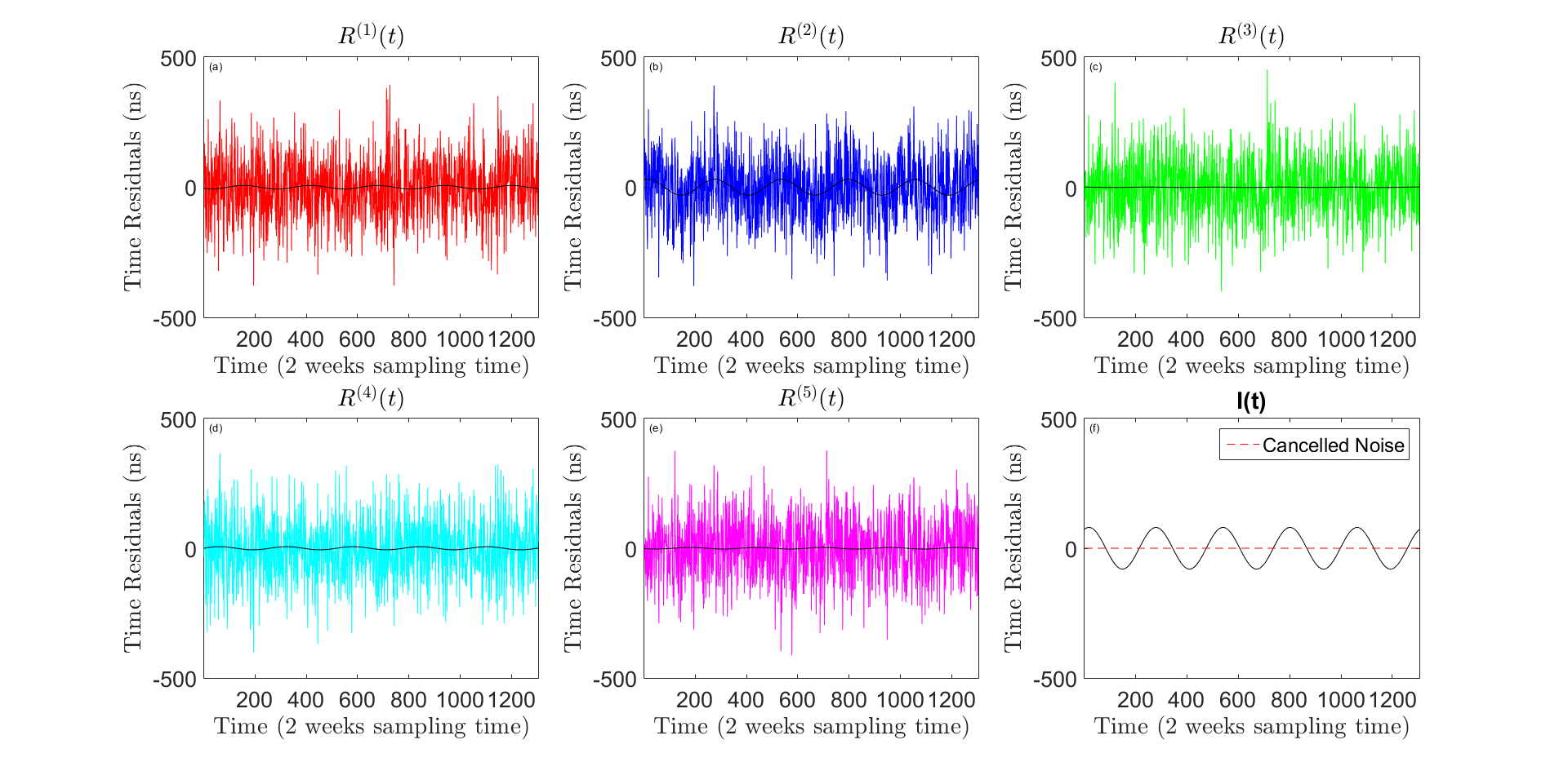
Figure 1: Simulation of the combination $I(t)$. The inserts (a) through (e) show five timing residuals containing a GW signal (black line) and noises from clock and ephemeris. The GW signal was assumed to be sinusoidal with frequency equal to $3.3\times 10^{-9}$ Hz, and with its two strain polarization amplitudes equal to $6.0\times 10^{-16}$ (each corresponding to about $30$ ns at the chosen frequency). The clock and ephemeris noises were taken to be Gaussian distributed random processes of zero-mean and r.m.s. amplitudes equal to $100$ ns (clock) and $100/\sqrt{3}$ ns for each of the three components of the ephemeris noise. The pulsars were assumed to be at a distance of 1 kpc and at some random directions in the sky; insert (f) shows $I(t)$ after applying the noise-canceling algorithm.

Although our analysis treats the pulsars’ sky locations as constants, it is clear that the linear combination $I(t)$ works with pulsars that may move across the sky. $I(t)$ should in fact be regarded as an example application of the more general data processing technique called Time-Delay Interferometry (TDI) Tinto and Dhurandhar (2014). By properly time-shifting and linearly combining data measured by a network of GW detectors, TDI provides the mathematical framework for deriving new time-series that are unaffected by correlated noises while retaining sensitivity to GWs.

III Sensitivity to Single-Source Signals

To quantify the advantages brought by our data processing technique, we will first derive the expression of the sensitivity to individual GW signals when $M=5$, and compare it against that of a single pulsar. To this end, let us first rewrite the expression of $I(t)$ in the following form

$$I(t)\equiv H(t)+N(t)=\sum_{r=1}^{5}\lambda_{r}H^{(r)}+\sum_{r=1}^{5}\lambda_{r}\zeta^{(r)}(t)\ ,$$ (15)

where $H(t)$ corresponds to the first term on the right-hand-side (the GW signal in $I$), and $N(t)$ to the second (the noise in $I$). To estimate the sensitivity of $I$ to individual GW signals, we first derive the expression of the GW signal power averaged over sources randomly distributed on the sky and polarization states

$$\langle|{\widetilde{H}}(f)|^{2}\rangle=\sum_{i,j=1}^{5}\lambda_{i}\lambda_{j}\langle{\widetilde{H}}^{(i)}(f){\widetilde{H}}^{*(j)}(f)\rangle=\sum_{i,j=1}^{5}\lambda_{i}\lambda_{j}\Theta^{ij}h^{2}(f)\ ,$$ (16)

where the angle-brackets denote the averaging operation over the celestial sphere and wave’s polarization states, $\widetilde{}$ represents the operation of Fourier transform and ^∗ that of complex conjugation. In Eq. (16) $\Theta^{ij}$ is the Hellings-Downs Hellings and Downs (1983) correlation function of the angle enclosed by the directions to the two pulsars ($i,j$), and $h^{2}(f)\equiv\langle|{\widetilde{H}}^{(i)}(f)|^{2}\rangle\ ,\ i=1,...5$, is the averaged GW power in each timing residual. This can be written as $h^{2}(f)=\rho^{2}(f)\ h^{2}_{0}(f)$, where $h_{0}(f)$ is the Fourier transform of the wave amplitude and $\rho(f)$ is the resulting wave’s r.m.s. transfer function to the pulsar response Estabrook and Wahlquist (1975); Armstrong et al. (1999); Jenet et al. (2011).

Since the noises $\zeta^{(r)}\ ,r=1,...5$ are uncorrelated and each can be characterized by its own one-sided power spectral density, $P_{\zeta^{(r)}}(f)$, the expression of the one-sided power spectral density of the noise $N$, $P_{N}(f)$, is equal to

$$P_{N}(f)=\sum_{r=1}^{5}\lambda^{2}_{r}P_{\zeta^{(r)}}(f)\ .$$ (17)

The GW sensitivity of the $I(t)$ combination, $\gamma(f)$, defined as the ratio between the square-root of its noise spectrum, $P_{N}(f)$, and the r.m.s. transfer function of its GW response, $\sqrt{\sum_{i,j=1}^{5}\lambda_{i}\lambda_{j}\Theta^{ij}\rho^{2}}$, is then equal to Thorne (1987); Armstrong et al. (1999)

$$\gamma(f)=\sqrt{\frac{\sum_{r=1}^{5}\lambda^{2}_{r}P_{\zeta^{(r)}}(f)}{\sum_{i,j=1}^{5}\lambda_{i}\lambda_{j}\Theta^{ij}\rho^{2}(f)}}\ .$$ (18)

To get some insights about $\gamma(f)$, let us consider the case of timing residual noises $\zeta^{(r)}$ being characterized by the same spectrum, i.e. $P_{\zeta}(f)\equiv P_{\zeta^{(r)}}(f)\ \ \ ,r=1,...5$. Under this assumption Eq.(18) assumes the following form

$$\gamma(f)=\sqrt{\frac{\sum_{r=1}^{5}\lambda^{2}_{r}}{\sum_{i,j=1}^{5}\lambda_{i}\lambda_{j}\Theta^{ij}}}\ \frac{\sqrt{P_{\zeta}(f)}}{\rho(f)}\ .$$ (19)

If we denote with ($\Theta_{min},\Theta_{max}$) the minimum and maximum values of the Hellings-Downs curve Hellings and Downs (1983) when $i\neq j$, and use the identity $\sum_{r=1}^{5}\lambda^{2}_{r}=-\sum_{i\neq j=1}^{5}\lambda_{i}\lambda_{j}$ (which follows from the first equation fulfilled by $\vec{\lambda}$ in Eq.(10)), from Eq. (19) it is then possible to derive the following inequality

$$\gamma_{max}>\gamma(f)>\gamma_{min}\ \ ,\ \ \gamma_{(min,max)}\equiv\frac{1}{\sqrt{1-\Theta_{(min,max)}}}\ \frac{\sqrt{P_{\zeta}(f)}}{\rho(f)}\ .$$ (20)

If we now multiply and divide the right-hand-side of Eq.(20) by the square-root of the one-sided power spectral density of the noise of each timing residual, $P_{R}(f)$, we derive the following upper-limit for the function $\gamma(f)$

$$\gamma(f)<\gamma_{max}=\frac{1}{\sqrt{1-\Theta_{max}}}\ \left(\sqrt{\frac{P_{\zeta}(f)}{P_{R}(f)}}\right)\ \left(\frac{\sqrt{P_{R}(f)}}{\rho(f)}\right)\ .$$ (21)

Since $\Theta_{min}\simeq-0.15$ and $\Theta_{max}\simeq 0.5$ Hellings and Downs (1983), the factor that determines the sensitivity gain of the clock- and ephemeris-free combination $I(t)$ over that of a single pulsar is the ratio $\sqrt{\frac{P_{\zeta}(f)}{P_{R}(f)}}$. This function of the Fourier frequency can be significantly smaller than one in the lower part of the band where clock and ephemeris noises dominate the noise budget. Based on the noise-model discussed in Jenet et al. (2011), in Fig. 2 we plot the estimated GW sensitivity of single-pulsar experiments together with the sensitivity bounds achievable by the noise-canceling combination $I(t)$ given in Eq. (20). In this figure we have assumed (i) use of multiple-frequency measurements to adequately calibrate timing fluctuations from intergalactic and interplanetary plasma, and (ii) disregarded the timing fluctuations due to the pulsars. Stability analysis of known millisecond pulsars Verbiest et al. (2009); Liu (2012) have shown that there exist some displaying frequency stabilities superior to those of the most stable operational clocks in the ($10^{-9}-10^{-8}$) Hz frequency band.

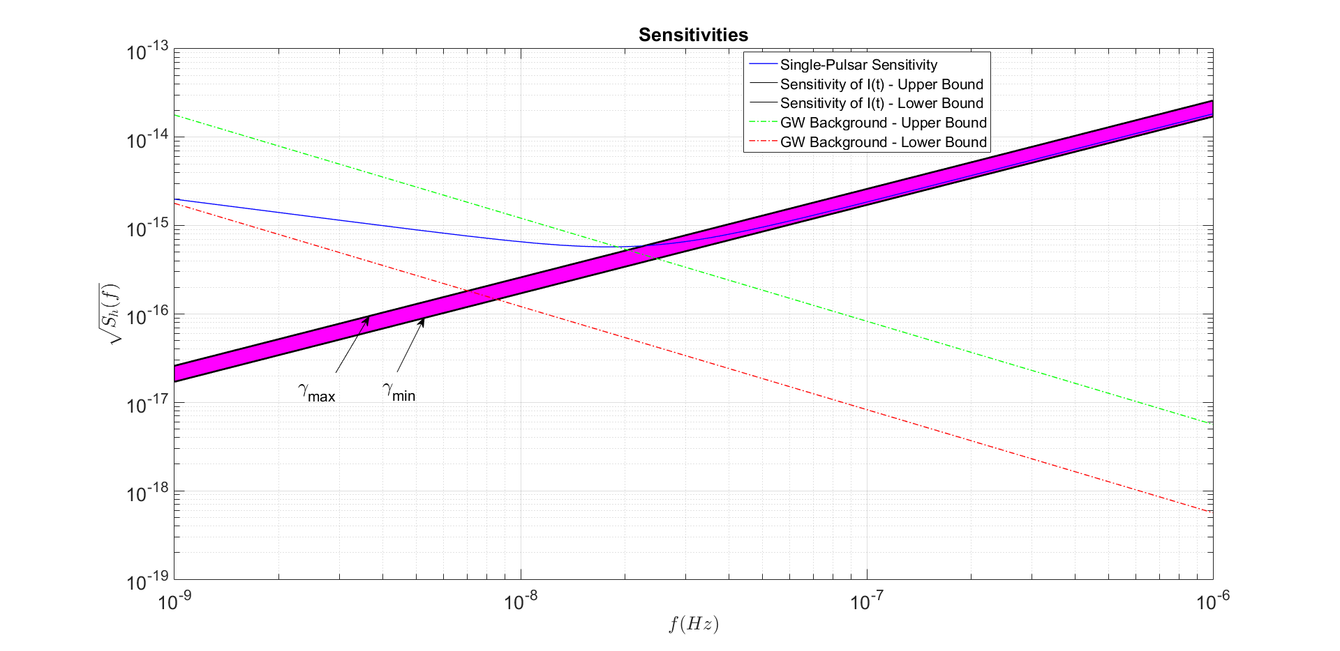
Figure 2: Gravitational wave sensitivity expressed as the ratio between the square-root of the one-sided power spectral density of the noise and the r.m.s. of the GW signal transfer function. The pulsars have been assumed to be at equal distances from Earth (1 kpc). The sensitivity of a single-telescope experiment (blue curve), as well as the current estimates of the upper- and lower-bounds (green and red line respectively) on the amplitude radiated by an ensemble of super-massive black-hole binaries are included Sesana et al. (2008); Arzoumanian and et al (2018a). Note the narrowness of the sensitivity region (bounded by the functions $\gamma_{max},\gamma_{min}$) within which the sensitivity of the data combination $I(t)$ is defined. The GW sensitivity gains of $I(t)$ over that of a single-pulsar experiment are evident in the frequency interval ($10^{-9}-2.0\times 10^{-8}$) Hz. The sensitivity curves presume adequate calibration of timing fluctuations from intergalactic and interplanetary plasma and negligible pulsars spin noises. See text for details.

As a final remark, arrays with $M\geq 5$ pulsars are characterized by Kernels of dimensionality equal to $M-4$ (as they have $M-4$ generators) and four-dimensional Images. When $M>5$ in particular, the sensitivity of single-source searches can be coherently improved over that with five pulsars by diagonalizing the correlation matrix associated with the resulting $M-4$ combinations that are clock- and ephemeris- free. The anticipated sensitivity enhancement is somewhat larger than $\sqrt{M-4}$, and we refer the reader to Prince et al. (2002) for details.

IV Sensitivity to an Isotropic Stochastic GW Background

The technique presented in this article for canceling correlated noises (such as clock and ephemeris) affecting data from pulsar timing arrays becomes particularly effective when searching for a stochastic background of gravitational radiation with an array of at least $10$ pulsars. This is because arrays with $10$ or more pulsars can generate pairs of clock- and ephemeris-free combinations whose noises are expected to be uncorrelated by not sharing data from the same pulsars. Since the kernel of clock- and ephemeris- free combinations generated by $M$ pulsars has dimensionality equal to $M-4$, we need to determine the number of pairs of combinations that can be constructed with the $M-4$ generators of the kernel and whose noises are uncorrelated.

To better understand the problem, let us first consider the case of $10$ pulsars. The associated kernel space is defined by $6$ generators, i.e. any clock- and ephemeris-free combination can be written as a linear combination of them. If we label the pulsars as ($1,2,\dots 10$), we can choose, for instance, the generators constructed by combining the following six set of $5$ pulsars $(1,2,3,4,5),(6,7,8,9,10),(2,3,4,5,6),(7,8,9,10,1),(3,4,5,6,7),(8,9,10,1,2)$, which were obtained by “circularly-right-shifting” to the right the ($1,2,\dots 10$) indices. With these generators we can only form the following three pairs of combinations whose noises are uncorrelated, $[(1,2,3,4,5),(6,7,8,9,10)]$ ; $[(2,3,4,5,6),(7,8,9,10,1)]$ ; $[(3,4,5,6,7),(8,9,10,1,2)]$, and implement with them the correlation statistic to search for a GW stochastic background.

Let us consider one of the above three pairs and denote with (${}^{(a)}I(t),{}^{(a)}{\bar{I}}(t)$) the corresponding two clock- and ephemeris-free combinations . Here ${}^{(a)}{\bar{I}}(t)$ contains TOA residuals that are not entering in the ${}^{(a)}I(t)$ combination and, from Eq. (15), both combinations can be written in the following forms

$${}^{(a)}I(t) \equiv {}^{(a)}H(t)+{}^{(a)}\zeta(t)=\sum_{j=1}^{5}{}^{(a)}\lambda_{j}{}^{(a)}H^{(j)}+\sum_{j=1}^{5}{}^{(a)}\lambda_{j}{}^{(a)}\zeta^{(j)}(t)\ ,$$

$${}^{(a)}{\bar{I}}(t) \equiv {}^{(a)}{\bar{H}}(t)+{}^{(a)}{\bar{\zeta}}(t)=\sum_{j=1}^{5}{}^{(a)}{\bar{\lambda}}_{j}{}^{(a)}{\bar{H}}^{(j)}+\sum_{j=1}^{5}{}^{(a)}{\bar{\lambda}}_{j}{}^{(a)}{\bar{\zeta}}^{(j)}(t)\ .$$ (22)

Since the noises in these two TOA residual combinations are uncorrelated, we can implement with them the cross-correlation statistic Wainstein and Zubakov (1962); Allen and Romano (1999) to search for a stochastic GW background. To keep as close as possible to the literature on the implementation of the correlation statistic for GW searches, we will formulate it in the Fourier domain . In what follows we will assume a GW background that is an isotropic, unpolarized, stationary, and Gaussian random process with zero mean. Such a background can be characterized by a one-sided power spectral density, $P_{h}(|f|)$, defined through the following expressions Allen and Romano (1999); Papoulis (2002)

$$\langle{}^{(a)}{\widetilde{H}}^{(i)}(f)\ {}^{(a)}{\widetilde{H}}^{*(j)}(f^{\prime})\rangle \equiv \frac{1}{2}\delta(f-f^{\prime}){}^{(a)}\Theta^{ij}\ P_{h}(|f|)\ ,$$

$$\langle{}^{(a)}{\widetilde{\bar{H}}}^{(i)}(f)\ {}^{(a)}{\widetilde{\bar{H}}}^{*(j)}(f^{\prime})\rangle \equiv \frac{1}{2}\delta(f-f^{\prime}){}^{(a)}{\bar{\Theta}}^{ij}\ P_{h}(|f|)\ ,$$

$$\langle{}^{(a)}{\widetilde{H}}^{(i)}(f)\ {}^{(a)}{\widetilde{\bar{H}}}^{*(j)}(f^{\prime})\rangle \equiv \frac{1}{2}\delta(f-f^{\prime}){}^{(a)}\Gamma^{ij}\ P_{h}(|f|)\ ,$$ (23)

where angle-brackets, $\langle\rangle$, now denote the operation of ensemble averaging of the random process and averaging over the celestial sphere and polarization states, and the three coefficients (${}^{(a)}\Theta^{ij},{}^{(a)}{\bar{\Theta}}^{ij},{}^{(a)}\Gamma^{ij}$) are the Hellings-Downs functions Hellings and Downs (1983) associated with the correlation of pairs of timing residuals in ${}^{(a)}I(t)$, ${}^{(a)}{\bar{I}}(t)$, and from both combinations respectively . Note that the spectrum $P_{h}(|f|)$ appearing in Eq. (23) depends on the spectrum of the GW background, $\Omega_{gw}(f)$, as well as on the r.m.s. transfer function, $\rho(f)$, of the GW background to the TOA residual response in the following way Allen and Romano (1999)

$$P_{h}(|f|)=\rho^{2}(f)\ \frac{3H_{0}^{2}}{32\pi^{3}}|f|^{-3}\Omega_{gw}(f)\ ,$$ (24)

where $H_{0}$ is the Hubble constant (today). The typical functional form for the GW spectrum is a power law, i.e. $\Omega_{gw}(f)\equiv\Omega_{\alpha}f^{\alpha}$. The spectral index $\alpha$ characterizes the shape of the GW spectrum and is the unknown to be determined by the filtering procedure described below.

We will further assume the random processes ${}^{(a)}\zeta^{(i)}$, ${}^{(a)}{\bar{\zeta}}^{(j)}$ to be stationary, Gaussian distributed with zero-mean, and characterized by the one-sided power spectral densities, ($P_{{}^{(a)}\zeta^{(j)}}(|f|)\ ,\ P_{{}^{(a)}{\bar{\zeta}}^{(j)}}(|f|)$), defined as follows

$$\langle{}^{(a)}{\widetilde{\zeta}}^{(i)}(f)\ {}^{(a)}{\widetilde{\zeta}}^{*(j)}(f^{\prime})\rangle \equiv \frac{1}{2}\delta^{ij}\ \delta(f-f^{\prime})\ P_{{}^{(a)}\zeta^{(i)}}(|f|)$$

$$\langle{}^{(a)}{\widetilde{\bar{\zeta}}}^{(i)}(f)\ {}^{(a)}{\widetilde{\bar{\zeta}}}^{*(j)}(f^{\prime})\rangle \equiv \frac{1}{2}\delta^{ij}\ \delta(f-f^{\prime})\ P_{{}^{(a)}{\bar{\zeta}}^{(i)}}(|f|)$$

$$\langle{}^{(a)}{\widetilde{\zeta}}^{(i)}(f)\ {}^{(a)}{\widetilde{\bar{\zeta}}}^{*(j)}(f^{\prime})\rangle \equiv 0\ ,$$ (25)

where $\delta^{ij}$ is the Kronecker symbol and $\delta(f-f^{\prime})$ is the Dirac’s delta function.

The sample cross-correlation statistic is defined as

$${}^{(a)}{\mathcal{S}}\equiv\int_{-T/2}^{T/2}dt\ \int_{-\infty}^{\infty}dt^{\prime}\ {}^{(a)}I(t){}^{(a)}{\bar{I}}(t^{\prime}){}^{(a)}Q(t-t^{\prime})\ ,$$ (26)

where ${}^{(a)}Q(t-t^{\prime})$ is the optimal filter that is non-zero over the time interval ($-T/2,T/2$) (a property we have already taken into account in Eq.(26) by extending the $t^{\prime}$ integration over the entire real axis), and reflects the stationarity of both the stochastic background and the instrumental noises by depending on time differences Allen and Romano (1999).

From the statistical properties of both the GW stochastic background and the noises, and by virtue of the central-limit theorem, it follows that ${}^{(a)}{\mathcal{S}}$ is also a Gaussian random process Papoulis (2002) that can be fully characterized by estimating its mean, ${}^{(a)}\mu_{\mathcal{S}}$, and variance, ${}^{(a)}\sigma_{\mathcal{S}}^{2}$. Although their derivations are long (see appendix (A) for details), they are straightforward and result in the following expressions

$${}^{(a)}\mu_{\mathcal{S}}\equiv\frac{T}{2}\int^{+\infty}_{-\infty}{}^{(a)}\Lambda(|f|)\ {}^{(a)}{\widetilde{Q}}(f)\ df=\frac{T}{2}\int^{+\infty}_{-\infty}\sum_{r,s=1}^{5}{}^{(a)}\lambda_{r}{}^{(a)}{\bar{\lambda}}_{s}{}^{(a)}\Gamma^{rs}P_{h}(|f|)\ {}^{(a)}{\widetilde{Q}}(f)\ df\ ,$$ (27)

$${}^{(a)}\sigma_{\mathcal{S}}^{2} \equiv \frac{T}{4}\int^{+\infty}_{-\infty}\Delta(|f|)\ |{}^{(a)}{\widetilde{Q}}(f)|^{2}\ df$$ (28)

$$= \frac{T}{4}\int^{+\infty}_{-\infty}\left[\sum_{r,s,p,q=1}^{5}[{}^{(a)}\lambda_{r}{}^{(a)}\lambda_{s}{}^{(a)}{\bar{\lambda}}_{p}{}^{(a)}{\bar{\lambda}}_{q}\ {}^{(a)}\Theta^{rs}\ {}^{(a)}{\bar{\Theta}}^{pq}+{}^{(a)}\lambda_{r}{}^{(a)}{\bar{\lambda}}_{s}{}^{(a)}\lambda_{p}{}^{(a)}{\bar{\lambda}}_{q}\ {}^{(a)}\Gamma^{rs}\ {}^{(a)}\Gamma^{pq}]\ P^{2}_{h}(|f|)\right.$$

$$+ \left.\sum_{r,s,q=1}^{5}[{}^{(a)}\lambda_{r}{}^{(a)}\lambda_{s}{}^{(a)}{\bar{\lambda}}^{2}_{q}\ {}^{(a)}\Theta^{rs}\ P_{{}^{(a)}{\bar{\zeta}}^{(q)}}(|f|)+{}^{(a)}{\bar{\lambda}}_{r}{}^{(a)}{\bar{\lambda}}_{s}{}^{(a)}\lambda^{2}_{q}\ {}^{(a)}{\bar{\Theta}}^{rs}\ P_{{}^{(a)}\zeta^{(q)}}(|f|)]\ P_{h}(|f|)\right.$$

$$+ \left.\sum_{r,s=1}^{5}{}^{(a)}\lambda_{r}^{2}\ {}^{(a)}{\bar{\lambda}}^{2}_{s}\ P_{{}^{(a)}\zeta^{(r)}}(|f|)\ P_{{}^{(a)}{\bar{\zeta}}^{(s)}}(|f|)\right]\ |{}^{(a)}{\widetilde{Q}}(f)|^{2}\ df\ .$$

By simple inspection of Eq. (28), and following Allen and Romano (1999), it is convenient to define the following operation of inner product between two arbitrary complex functions, say $A$, and $B$

$$(A,B)\equiv\int^{+\infty}_{-\infty}A(f)B^{*}(f)\Delta(|f|)\ df\ .$$ (29)

With this newly defined inner product, ${}^{(a)}\mu_{\mathcal{S}}$ and ${}^{(a)}\sigma_{\mathcal{S}}$ can be rewritten in the following forms

$${}^{(a)}\mu_{\mathcal{S}}=\frac{T}{2}({}^{(a)}{\widetilde{Q}},\frac{{}^{(a)}\Lambda}{{}^{(a)}\Delta})\ \ \ \ ;\ \ \ \ {}^{(a)}\sigma^{2}_{\mathcal{S}}=\frac{T}{4}({}^{(a)}{\widetilde{Q}}(f),{}^{(a)}{\widetilde{Q}}(f))\ ,$$ (30)

while the squared signal-to-noise ratio of ${}^{(a)}{\mathcal{S}}$, ${}^{(a)}SNR^{2}$, is equal to

$${}^{(a)}SNR^{2}\equiv\frac{{}^{(a)}\mu_{\mathcal{S}}^{2}}{{}^{(a)}\sigma_{\mathcal{S}}^{2}}=T\ \frac{({}^{(a)}{\widetilde{Q}},\frac{{}^{(a)}\Lambda}{{}^{(a)}\Delta})^{2}}{({}^{(a)}{\widetilde{Q}},{}^{(a)}{\widetilde{Q}})}\ .$$ (31)

From a simple geometrical interpretation of the inner product defined through Eq. (29), from Eq. (31) we conclude that the maximum of the SNR of ${}^{(a)}{\mathcal{S}}$ is achieved by choosing the filter function ${}^{(a)}{\widetilde{Q}}$ to be equal to

$${}^{(a)}{\widetilde{Q}}(f)={}^{(a)}{\xi}\ \frac{{}^{(a)}\Lambda}{{}^{(a)}\Delta}\ ,$$ (32)

where ${}^{(a)}{\xi}$ is an arbitrary real number and, from the definition of the functions ${}^{(a)}\Lambda$ and ${}^{(a)}\Delta$ (Eqs. 27, 28), it also follows that ${}^{(a)}{\widetilde{Q}}(f)$ is real. We can take advantage of the arbitrariness of ${}^{(a)}{\xi}$ by making all mean values of the cross-correlations equal to the following constant $\mu_{\mathcal{S}}\equiv{}^{(a)}\mu_{\mathcal{S}}=\Omega_{\alpha}\ T\ ,\ a=1,2,3$ Allen and Romano (1999). As it will become clearer later on in this section, this choice simplifies the derivation of the coherent SNR achievable by properly combining the cross-correlations of pairs of clock- and ephemeris-free combinations.

The expression for the filter ${}^{(a)}{\widetilde{Q}}$ given by Eq. (32) implies the following maximum SNR achievable by cross-correlating the pair (${}^{(a)}I(t),{}^{(a)}{\bar{I}}(t)$)

$${}^{(a)}SNR_{{}^{(a)}I}\equiv\sqrt{T}\ \sqrt{\int^{+\infty}_{-\infty}\frac{{}^{(a)}\Lambda^{2}(|f|)}{{}^{(a)}\Delta(|f|)}\ df}\ .$$ (33)

In the limit in which the noise spectra of the TOA residuals are larger than that of the GW background, the integrand of Eq.(33) becomes equal to

$$\frac{{}^{(a)}\Lambda^{2}(|f|)}{{}^{(a)}\Delta(|f|)}\simeq\frac{\left(\sum_{r,s=1}^{5}{}^{(a)}\lambda_{r}{}^{(a)}{\bar{\lambda}}_{s}\Gamma^{rs}\right)^{2}\ P^{2}_{h}(|f|)}{\left(\sum_{r=1}^{5}{}^{(a)}\lambda^{2}_{r}P_{{}^{(a)}\zeta^{(r)}}(|f|)\right)\ \left(\sum_{s=1}^{5}{}^{(a)}{\bar{\lambda}}^{2}_{s}P_{{}^{(a)}{\bar{\zeta}}^{(s)}}(|f|)\right)}\ .$$ (34)

Note that the above expression of the optimal SNR depends on the pulsars’ relative sky locations through the Hellings and Downs correlation function and the vectors, ${{}^{(a)}{\vec{\lambda}}},{{}^{(a)}{\bar{\vec{\lambda}}}}$ identifying the pulsars’ clock- and ephemeris-free combinations. To quantify the angular dependence of the optimal SNR, we can assume the timing residual noises (${}^{(a)}\zeta^{(r)},{}^{(a)}{\bar{\zeta}}^{(r)}\ ,\ r=1,\dots 5$) to be characterized by the same spectrum, $P_{\zeta}(|f|)$. Under this assumption the optimal SNR becomes equal to

$${}^{(a)}SNR_{{}^{(a)}I}\equiv\sqrt{T}\ \frac{|\sum_{r,s=1}^{5}{}^{(a)}\lambda_{r}{}^{(a)}{\bar{\lambda}}_{s}\Gamma^{rs}|}{\sqrt{\sum_{r,s=1}^{5}{}^{(a)}\lambda^{2}_{r}{}^{(a)}{\bar{\lambda}}^{2}_{s}}}\sqrt{\int^{+\infty}_{-\infty}\frac{P^{2}_{h}(|f|)}{P_{\zeta}^{2}(|f|)}\ df}\ ,$$ (35)

where the dependence of the SNR on the pulsars’ relative sky locations can now be factored out of the integral. To quantify the magnitude of the angular function appearing in Eq. (35) we have randomly generated $10^{7}$ sets of $10$ pulsars’ sky locations and compute it for each set. We found the above angular function to assume values within the interval ($0,1$) and to have an r.m.s. value equal to about $1/5$.

To compare the effectiveness of our cross-correlation statistic against that based on a pair of TOA residuals, ($R^{(i)}(t),R^{(j)}(t)$), we provide below the expression for the optimal SNR, $SNR^{ij}_{R}$, associated with the cross-correlation statistic of two timing residuals

$$SNR^{ij}_{R}=\sqrt{T}\sqrt{\int^{+\infty}_{-\infty}df\ \frac{[\Gamma^{ij}P_{h}(|f|)+P_{C}(|f|)+P_{e^{ij}}(|f|)]^{2}}{\Pi(|f|)}}\ ,$$ (36)

where:

$$\Pi(|f|) \equiv 2P^{2}_{C}(|f|)+P_{e^{ii}}(|f|)P_{e^{jj}}(|f|)+P^{2}_{e^{ij}}(|f|)+[P_{e^{ii}}(|f|)+P_{e^{jj}}(|f|)]P_{\zeta}(|f|)$$ (37)

$$+ [P_{e^{ii}}(|f|)+P_{e^{jj}}(|f|)+2P_{e^{ij}}(|f|)+2P_{\zeta}(|f|)]P_{C}(|f|)+P^{2}_{\zeta}(|f|)\ .$$

Eqs. (36, 37) reflect the assumption on the spectra of the $\zeta$-noises to be equal to each other and larger than the GW background, and where we have also denoted with ($P_{C}(|f|),P_{e^{ij}}(|f|)$) the spectra of the clock and ephemeris noises respectively. Eqs. (36, 37) allow us to quantify two aspects of the degradation in the likelihood of detection due to correlated-noises in pulsar timing data Coles et al. (2011); Tiburzi et al. (2016); Arzoumanian and et al (2018a). First, the cross-correlation statistic of pairs of TOA residuals from different pulsars is affected by clock and ephemeris noises through their contribution to the mean value of the cross-correlation (i.e. the numerator of the integrand in Eq. (36)). Since these noises are characterized by relatively large spectral components in the same part of the band associated with the presence of a stochastic GW background, they result in an increased false-alarm probability . Second, clock and ephemeris noises contribute to the overall noise variance of the TOA residuals and therefore reduce (by a factor larger than $10$ Jenet et al. (2011)) the optimal cross-correlation SNR (Eq. (36)) over that associated with pairs of clock and ephemeris-free combinations (Eq. (35)).

Following Allen and Romano (1999), we now provide the expression for the SNR achievable by optimally combining the three pairs of clock- and ephemeris-free combinations that can be synthesized with the timing data from an array of $10$ pulsars. This requires the calculation of the inverse of the variance-covariance matrix of the cross-correlation statistic, ${}^{(ab)}C\equiv\langle{}^{(a)}{\mathcal{S}}{}^{(b)}{\mathcal{S}}\rangle-\langle{}^{(a)}{\mathcal{S}}\rangle\ \langle{}^{(b)}{\mathcal{S}}\rangle$. The discussion on how to derive ${}^{(ab)}C$ is presented in the appendix, and its expression can be written in the following form

$${}^{(ab)}C = \frac{T}{4}\int^{+\infty}_{-\infty}\left[\sum_{r,s,p,q=1}^{5}[{}^{(a)}\lambda_{r}{}^{(b)}\lambda_{s}{}^{(a)}{\bar{\lambda}}_{p}{}^{(b)}{\bar{\lambda}}_{q}{}^{(ab)}\Theta^{rs}{}^{(ab)}{\bar{\Theta}}^{pq}+{}^{(a)}\lambda_{r}{}^{(b)}{\bar{\lambda}}_{s}{}^{(a)}{\bar{\lambda}}_{p}{}^{(b)}\lambda_{q}{}^{(ab)}\Gamma^{rs}{}^{(ab)}{\bar{\Gamma}}^{pq}]\ P^{2}_{h}(|f|)\right.$$ (38)

$$+ \left.\sum_{r,s,p,q=1}^{5}[{}^{(a)}\lambda_{r}{}^{(b)}\lambda_{s}{}^{(a)}{\bar{\lambda}}_{p}{}^{(b)}{\bar{\lambda}}_{q}{}^{(ab)}\Theta^{rs}\eta^{(ab)}_{pq}\ {}^{(ab)}P_{{\bar{\zeta}}_{p}}(|f|)+{}^{(a)}\lambda_{r}{}^{(b)}\lambda_{s}{}^{(a)}{\bar{\lambda}}_{p}{}^{(b)}{\bar{\lambda}}_{q}{}^{(ab)}{\bar{\Theta}}^{pq}\eta^{(ab)}_{rs}\ {}^{(ab)}P_{{\zeta}_{r}}(|f|)\right.$$

$$+ \left.{}^{(a)}\lambda_{r}{}^{(b)}{\bar{\lambda}}_{s}{}^{(a)}{\bar{\lambda}}_{p}{}^{(b)}\lambda_{q}{}^{(ab)}\Gamma^{rs}\eta^{(ab)}_{pq}\ {}^{(ab)}P_{{\zeta}_{p}}(|f|)+{}^{(a)}\lambda_{r}{}^{(b)}{\bar{\lambda}}_{s}{}^{(a)}{\bar{\lambda}}_{p}{}^{(b)}\lambda_{q}{}^{(ab)}\Gamma^{pq}\eta^{(ab)}_{rs}\ {}^{(ab)}P_{{\bar{\zeta}}_{r}}(|f|)]\ P_{h}(|f|)\right.$$

$$+ \left.\sum_{r,s,p,q=1}^{5}{}^{(a)}\lambda_{r}{}^{(b)}{\bar{\lambda}}_{s}{}^{(a)}{\bar{\lambda}}_{p}{}^{(b)}\lambda_{q}\eta^{(ab)}_{rs}\eta^{(ab)}_{pq}\ {}^{(ab)}P_{{\bar{\zeta}}_{r}}(|f|)\ {}^{(ab)}P_{{\zeta}_{p}}(|f|)\right]\ {}^{(a)}{\widetilde{Q}}(f){}^{(b)}{\widetilde{Q}}^{*}(f)\ df\ .$$

In the above equation the multi-indices symbol $\eta^{(ab)}_{pq}$ is either equal to $0$ or $1$ depending on the particular outcome of the correlation of two $\zeta$ noises entering in the combinations’ pair $(ab)$, and it reduces to $\delta_{pq}$ when $a=b$. The expression for the optimal SNR achievable by combining the cross-correlations of our three pairs of clock- and ephemeris-free combinations is equal to Allen and Romano (1999)

$$SNR_{opt}^{2}=({}^{(1)}\mu_{\mathcal{S}},{}^{(2)}\mu_{\mathcal{S}},{}^{(3)}\mu_{\mathcal{S}})\ C^{-1}\ ({}^{(1)}\mu_{\mathcal{S}},{}^{(2)}\mu_{\mathcal{S}},{}^{(3)}\mu_{\mathcal{S}})^{\mathcal{T}}=(\Omega_{\alpha}T)^{2}\ \sum_{a,b=1}^{3}{}^{(ab)}(C^{-1})\ ,$$ (39)

where the mean values ${}^{(i)}\mu_{\mathcal{S}}\ ,\ i=1,2,3$ have been normalized to the same constant value $\Omega_{\alpha}T$.

The analysis for a set of $10$ pulsars presented above can be generalized to an arbitrary array of size $M$. This is done by first selecting the $M-4$ generators of the kernel, and then identifying the set of all pairs of generators that do not have pulsars in common, i.e. pairs of clock- and ephemeris-free combinations whose noises are uncorrelated. As an example of how to identify such set of generators’ pairs, let us consider an array with $45$ pulsars, equal in number to the array recently analyzed by the NANOGRAV consortium Arzoumanian and et al (2018b). Let us first consider the numerical vector ($1,2,\dots 45$), which can be used to label the $45$ pulsars. If we use the “right-circular-shifting” procedure described earlier for selecting a set of generators of the $10$-pulsar kernel, we obtain the following $41$ generators

$$( 1,\dots 5),(6,\dots 10)\dots(41,\dots 45)$$ (40)

$$( 45,\dots 4),(5,\dots 9)\dots(40,\dots 44)$$

$$( 44,\dots 3),(4,\dots 8)\dots(39,\dots 43)$$

$$( 43,\dots 2),(3,\dots 7)\dots(38,\dots 42)$$

$$( 42,\dots 1),(2,\dots 6),(7,\dots 11),(12,\dots 16),(17,\dots 21)$$

This set of $41$ clock- and ephemeris-free combinations of timing residuals results in a total of $672$ pairs that do not share data from the same pulsars, and can therefore be used to implement the cross-correlation statistic. Since this number is comparable to the number of pairs ($990$) of timing residuals given by an array $45$ pulsars (and upon which the usual cross-correlation statistic is built), it follows that the optimal SNRs associated with both cross-correlation statistics will scale roughly by the same amount over their respective single-pair SNRs Allen and Romano (1999).

V Conclusions

The data processing technique presented in this article allows us to cancel clock and ephemeris noises affecting nHz GW pulsar timing experiments. This is done by properly constructing linear combinations of TOA residuals generated by arrays of millisecond pulsars.

We have found that searches for single-source GW signals will benefit from this technique when implemented with arrays of at least $5$ millisecond pulsars. The estimated sensitivity enhancement over that from individual pulsar experiments is of at least one order of magnitude in the lower-part of the accessible frequency band. This is the frequency region where clock and ephemeris noises are leading noise sources equally effecting the array’s timing measurements.

Searches for an isotropic stochastic GW background can also be performed with clock- and ephemeris-free combinations from an array of $10$ or more pulsars. This is done by implementing the cross-correlation statistic with pairs of clock- and ephemeris-free combinations that do not share timing residuals from the same pulsars to prevent noise correlations. With an array of $10$ pulsars we have found the associated cross-correlation statistic to be characterized by an optimal SNR that is more than an order of magnitude larger than the optimal SNR achievable by cross-correlating pairs of timing residuals from an equal-size array.

As a final note, we have shown that clock and ephemeris noises can be reconstructed with the timing data from an array of $4$ or more pulsars. In a future article we will estimate the accuracies by which these observable can be reconstructed as functions of the number of pulsars, their relative sky locations, and the magnitudes of the remaining noises affecting the timing measurements.

Appendix A Derivation of the mean and variance-covariance of ${\mathcal{S}}$

In what follows we derive the expressions of the mean and the variance-covariance matrix of the cross-correlation function ${}^{(a)}S$ (Eqs. (27, 28, 38) given in Section (IV)) for an array of $10$ pulsars. We will assume the noises $\zeta_{r}$ to be Gaussian-distributed with zero-mean, and to have one-sided power-spectral densities $P_{\zeta_{r}}(|f|)$. We will also take the GW stochastic background to be a Gaussian random process of zero-mean, unpolarized, and stationary. As a consequence of these assumptions such a background is uniquely characterized by a one-sided power spectral density, $P_{h}(|f|)$ as given by Eqs. (23, 24).

From the expressions of the clock- and ephemeris-free data combinations, ${}^{(a)}I(t)$, their complements, ${}^{(a)}{\bar{I}}(t)$, (i.e. those combinations that do not include timing data from the pulsars entering in ${}^{(a)}I(t)$), and the definition of their cross-correlation statistic, ${}^{(a)}{\mathcal{S}}$, we have

$${}^{(a)}{\mathcal{S}}\equiv\int_{-T/2}^{T/2}dt\ \int_{-\infty}^{\infty}dt^{\prime}\ {}^{(a)}I(t){}^{(a)}{\bar{I}}(t^{\prime}){}^{(a)}Q(t-t^{\prime})\ ,$$ (41)

where ${}^{(a)}Q(t-t^{\prime})$ is the optimal filter. Since this is non-zero over the interval ($-T/2,T/2$), we have extended the $t^{\prime}$ integration over the entire real axis. Equivalently, Eq. (41) can be rewritten in the Fourier domain as follows

$${}^{(a)}{\mathcal{S}}=\int_{-\infty}^{\infty}df\ \int_{-\infty}^{\infty}df^{\prime}\ \delta_{T}(f-f^{\prime})\ {}^{(a)}{\widetilde{I}}^{*}(f){}^{(a)}{\widetilde{\bar{I}}}(f^{\prime}){}^{(a)}{\widetilde{Q}}(f^{\prime})\ ,$$ (42)

where $\delta_{T}(f)\equiv Tsinc(\pi fT)$ is the finite-time approximation of the Dirac’s delta function.

Since the noises in the combination ${}^{(a)}I(t)$ do not enter in ${}^{(a)}{\bar{I}}(t)$, and because a GW stochastic background is uncorrelated with the measurement noises, we infer that the ensemble average of the cross-correlation statistic, Eq. (42), contains contribution only from the GW stochastic background in the following form

$${}^{(a)}\mu_{\mathcal{S}}\equiv\langle{}^{(a)}{\mathcal{S}}\rangle = \int_{-\infty}^{\infty}df\ \int_{-\infty}^{\infty}df^{\prime}\ \delta_{T}(f-f^{\prime})\ \langle{}^{(a)}{\widetilde{I}}^{*}(f){}^{(a)}{\widetilde{\bar{I}}}(f^{\prime})\rangle{}^{(a)}{\widetilde{Q}}(f^{\prime})$$ (43)

$$= \int_{-\infty}^{\infty}df\ \int_{-\infty}^{\infty}df^{\prime}\ \delta_{T}(f-f^{\prime})\ \langle{}^{(a)}{\widetilde{H}}^{*}(f){}^{(a)}{\widetilde{\bar{H}}}(f^{\prime})\rangle{}^{(a)}{\widetilde{Q}}(f^{\prime})\ ,$$

where ${}^{(a)}{\widetilde{H}}^{*}(f)$, ${}^{(a)}{\widetilde{\bar{H}}}(f^{\prime})$ are the contributions of the GW stochastic background to the clock- and ephemeris-free combinations ${}^{(a)}{\widetilde{I}}^{*}(f)$, ${}^{(a)}{\widetilde{\bar{I}}}(f^{\prime})$ respectively. Since ${}^{(a)}{\widetilde{H}}^{*}(f)=\sum_{r=1}^{5}{}^{(a)}\lambda_{r}{}^{(a)}{\widetilde{H}}^{*r}(f)$, and ${}^{(a)}{\widetilde{\bar{H}}}(f^{\prime})=\sum_{r=1}^{5}{}^{(a)}{\bar{\lambda}}_{r}{}^{(a)}{\widetilde{\bar{H}^{r}}}(f)$, we have

$$\langle{}^{(a)}{\widetilde{H}}^{*}(f){}^{(a)}{\widetilde{\bar{H}}}(f^{\prime})\rangle = \sum_{r,s=1}^{5}{}^{(a)}\lambda_{r}{}^{(a)}{\bar{\lambda}}_{s}\langle{}^{(a)}{\widetilde{H}}^{*r}(f){}^{(a)}{\widetilde{\bar{H}^{s}}}(f^{\prime})\rangle$$ (44)

$$= \frac{1}{2}\delta(f-f^{\prime})\sum_{r,s=1}^{5}{}^{(a)}\lambda_{r}{}^{(a)}{\bar{\lambda}}_{s}{}^{(a)}\Gamma^{rs}\ {}^{(a)}P_{h}(|f|)\ ,$$

where ${}^{(a)}\Gamma^{rs}$ is the Hellings and Downs correlation function Hellings and Downs (1983). After substituting Eq. (44) into Eq. (43) and exercising the Dirac’s delta function, we finally obtain Eq. (27).

From the definition of the variance-covariance matrix of the cross-correlation statistic,

$${}^{(ab)}C\equiv\langle{}^{(a)}{\mathcal{S}}{}^{(b)}{\mathcal{S}}\rangle-\langle{}^{(a)}{\mathcal{S}}\rangle\langle{}^{(b)}{\mathcal{S}}\rangle\ ,$$ (45)

we have

$${}^{(ab)}C = \int_{-\infty}^{\infty}df\ \int_{-\infty}^{\infty}df^{\prime}\int_{-\infty}^{\infty}dk\ \int_{-\infty}^{\infty}dk^{\prime}\ \delta_{T}(f-f^{\prime})\ \delta_{T}(k-k^{\prime})$$ (46)

$$\times \ \left[\langle{}^{(a)}{\widetilde{I}}^{*}(f){}^{(a)}{\widetilde{\bar{I}}}(f^{\prime})\ {}^{(b)}{\widetilde{I}}(k){}^{(b)}{\widetilde{\bar{I}}}^{*}(k^{\prime})\rangle-\langle{}^{(a)}{\widetilde{I}}^{*}(f){}^{(a)}{\widetilde{\bar{I}}}(f^{\prime})\rangle\langle{}^{(b)}{\widetilde{I}}(k){}^{(b)}{\widetilde{\bar{I}}}^{*}(k^{\prime})\rangle\right]$$

$$\times \ {}^{(a)}{\widetilde{Q}}(f^{\prime}){}^{(b)}{\widetilde{Q}}^{*}(k^{\prime})\ .$$

Since the random processes associated with the noises and the GW background are Gaussian, we infer that the linear combinations ${}^{(a)}{\widetilde{I}}(f)$, ${}^{(a)}{\widetilde{\bar{I}}}(f^{\prime})$, ${}^{(b)}{\widetilde{I}}(f)$, ${}^{(b)}{\widetilde{\bar{I}}}(f^{\prime})$ are also Gaussian. This implies that the term in the integrand containing four $I$-combinations, inside the ensemble average operator, can be written in the following form Papoulis (2002)

$$\langle{}^{(a)}{\widetilde{I}}^{*}(f){}^{(a)}{\widetilde{\bar{I}}}(f^{\prime}){}^{(b)}{\widetilde{I}}(k){}^{(b)}{\widetilde{\bar{I}}}^{*}(k^{\prime})\rangle = \langle{}^{(a)}{\widetilde{I}}^{*}(f){}^{(a)}{\widetilde{\bar{I}}}(f^{\prime})\rangle\langle{}^{(b)}{\widetilde{I}}(k){}^{(b)}{\widetilde{\bar{I}}}^{*}(k^{\prime})\rangle$$ (47)

$$+ \langle{}^{(a)}{\widetilde{I}}^{*}(f){}^{(b)}{\widetilde{I}}(k)\rangle\langle{}^{(a)}{\widetilde{\bar{I}}}(f^{\prime}){}^{(b)}{\widetilde{\bar{I}}}^{*}(k^{\prime})\rangle$$

$$+ \langle{}^{(a)}{\widetilde{I}}^{*}(f){}^{(b)}{\widetilde{\bar{I}}}^{*}(k^{\prime})\rangle\langle{}^{(a)}{\widetilde{\bar{I}}}(f^{\prime}){}^{(b)}{\widetilde{I}}(k)\rangle$$

After substituting Eq. (47) into Eq. (46) we get

$${}^{(ab)}C = \int_{-\infty}^{\infty}df\ \int_{-\infty}^{\infty}df^{\prime}\int_{-\infty}^{\infty}dk\ \int_{-\infty}^{\infty}dk^{\prime}\ \delta_{T}(f-f^{\prime})\ \delta_{T}(k-k^{\prime})$$ (48)

$$\times \ \left[\langle{}^{(a)}{\widetilde{I}}^{*}(f){}^{(b)}{\widetilde{I}}(k)\rangle\langle{}^{(a)}{\widetilde{\bar{I}}}(f^{\prime}){}^{(b)}{\widetilde{\bar{I}}}^{*}(k^{\prime})\rangle+\langle{}^{(a)}{\widetilde{I}}^{*}(f){}^{(b)}{\widetilde{\bar{I}}}^{*}(k^{\prime})\rangle\langle{}^{(a)}{\widetilde{\bar{I}}}(f^{\prime}){}^{(b)}{\widetilde{I}}(k)\rangle\right]$$

$$\times \ {}^{(a)}{\widetilde{Q}}(f^{\prime}){}^{(b)}{\widetilde{Q}}^{*}(k^{\prime})\ .$$

By replacing the $I$s in terms of their GW signal and noise terms, and applying the ensemble average operation (see Eqs. (23, 25) on the resulting expressions entering in Eq. (48), Eq. (38) can be obtained after some straightforward algebra.

References

- Aasi and et al (2015) J. Aasi and et al (LIGO Scientific Collaboration), Classical and Quantum Gravity 32, 074001 (2015), URL http://stacks.iop.org/0264-9381/32/i=7/a=074001.
- Abbott and et al (2016a) B. P. Abbott and et al (LIGO Scientific Collaboration and Virgo Collaboration), Phys. Rev. Lett. 116, 061102 (2016a), URL https://link.aps.org/doi/10.1103/PhysRevLett.116.061102.
- Abbott and et al (2016b) B. P. Abbott and et al (LIGO Scientific Collaboration and Virgo Collaboration), Phys. Rev. Lett. 116, 241103 (2016b), URL https://link.aps.org/doi/10.1103/PhysRevLett.116.241103.
- Abbott and et al (2017a) B. P. Abbott and et al (LIGO Scientific and Virgo Collaboration), Phys. Rev. Lett. 118, 221101 (2017a), URL https://link.aps.org/doi/10.1103/PhysRevLett.118.221101.
- Abbott and et al (2017b) B. P. Abbott and et al (LIGO Scientific Collaboration and Virgo Collaboration), Phys. Rev. Lett. 119, 141101 (2017b), URL https://link.aps.org/doi/10.1103/PhysRevLett.119.141101.
- Abbott and et al (2017c) B. P. Abbott and et al (LIGO Scientific Collaboration and Virgo Collaboration), Phys. Rev. Lett. 119, 161101 (2017c), URL https://link.aps.org/doi/10.1103/PhysRevLett.119.161101.
- Amaro-Seoane and et al (2017) P. Amaro-Seoane and et al, ArXiv e-prints: https://arxiv.org/abs/1702.00786 (2017), eprint 1702.00786.
- Tinto and de Araujo (2016) M. Tinto and J. C. N. de Araujo, Phys. Rev. D 94, 081101 (2016), URL https://link.aps.org/doi/10.1103/PhysRevD.94.081101.
- Accadia and et al (2012) T. Accadia and et al, Journal of Instrumentation 7, P03012 (2012), URL http://stacks.iop.org/1748-0221/7/i=03/a=P03012.
- Armstrong (2006) J. W. Armstrong, Living Reviews in Relativity 9, 1 (2006), ISSN 1433-8351, URL https://doi.org/10.12942/lrr-2006-1.
- Estabrook and Wahlquist (1975) F. B. Estabrook and H. D. Wahlquist, General Relativity and Gravitation 6, 439 (1975), ISSN 1572-9532, URL https://doi.org/10.1007/BF00762449.
- Detweiler (1979) S. Detweiler, Astrophys. J. 234, 1100 (1979).
- Jenet et al. (2011) F. A. Jenet, J. W. Armstrong, and M. Tinto, Phys. Rev. D 83, 081301 (2011), URL https://link.aps.org/doi/10.1103/PhysRevD.83.081301.
- Tiburzi et al. (2016) C. Tiburzi, G. Hobbs, M. Kerr, W. A. Coles, S. Dai, R. N. Manchester, A. Possenti, R. M. Shannon, and X. P. You, Monthly Notices of the Royal Astronomical Society 455, 4339 (2016), URL +http://dx.doi.org/10.1093/mnras/stv2143.
- Arzoumanian and et al (2018a) Z. Arzoumanian and et al, ArXiv e-prints: https://arxiv.org/abs/1801.02617 (2018a), eprint 1801.02617.
- Arzoumanian and et al (2018b) Z. Arzoumanian and et al, ArXiv e-prints: https://arxiv.org/abs/1801.01837 (2018b), eprint 1801.01837.
- Burt et al. (2008) E. A. Burt, W. A. Diener, and R. L. Tjoelker, IEEE Transactions on Ultrasonics, Ferroelectrics, and Frequency Control 55, 2586 (2008), ISSN 0885-3010.
- Wyithe and Loeb (2003) J. S. B. Wyithe and A. Loeb, The Astrophysical Journal 590, 691 (2003), URL http://stacks.iop.org/0004-637X/590/i=2/a=691.
- Enoki et al. (2004) M. Enoki, K. T. Inoue, M. Nagashima, and N. Sugiyama, The Astrophysical Journal 615, 19 (2004), URL http://stacks.iop.org/0004-637X/615/i=1/a=19.
- Sesana et al. (2008) A. Sesana, A. Vecchio, and C. N. Colacino, Monthly Notices of the Royal Astronomical Society 390, 192 (2008), URL +http://dx.doi.org/10.1111/j.1365-2966.2008.13682.x.
- Schneider et al. (2010) R. Schneider, S. Marassi, and V. Ferrari, Classical and Quantum Gravity 27, 194007 (2010), URL http://stacks.iop.org/0264-9381/27/i=19/a=194007.
- Hellings and Downs (1983) R. W. Hellings and G. S. Downs, Astrophys. J. Lett. 265, L39 (1983).
- Jenet et al. (2005) F. A. Jenet, G. B. Hobbs, K. J. Lee, and R. N. Manchester, The Astrophysical Journal Letters 625, L123 (2005), URL http://stacks.iop.org/1538-4357/625/i=2/a=L123.
- Coles et al. (2011) W. Coles, G. Hobbs, D. J. Champion, R. N. Manchester, and J. P. W. Verbiest, Monthly Notices of the Royal Astronomical Society 418, 561 (2011), URL +http://dx.doi.org/10.1111/j.1365-2966.2011.19505.x.
- Kuchynka and Folkner (2013) P. Kuchynka and W. M. Folkner, Icarus 222, 243 (2013), ISSN 0019-1035, URL http://www.sciencedirect.com/science/article/pii/S0019103512004496.
- Lorimer and Kramer (2005) D. Lorimer and M. Kramer, Handbook of Pulsar Astronomy (Cambridge University Press, The Edinburgh Building, Cambridge CB2 2RU, UK, 2005), 1st ed., ISBN 978-0521828239.
- Madison et al. (2013) D. R. Madison, S. Chatterjee, and J. M. Cordes, The Astrophysical Journal 777, 104 (2013), URL http://stacks.iop.org/0004-637X/777/i=2/a=104.
- Laakso et al. (1996) T. I. Laakso, V. Valimaki, M. Karjalainen, and U. K. Laine, IEEE Signal Processing Magazine 13, 30 (1996), ISSN 1053-5888.
- Shaddock et al. (2004) D. A. Shaddock, B. Ware, R. E. Spero, and M. Vallisneri, Phys. Rev. D 70, 081101 (2004), URL https://link.aps.org/doi/10.1103/PhysRevD.70.081101.
- Wahlquist (1987) H. Wahlquist, Gen. Relativ. Gravit. 19, 1101 (1987), URL http://www.springerlink.com/content/k472327452285616.
- Lang (2004) S. Lang, Linear Algebra (Springer-Verlag, 175 Fifth Avenue, New York, NY, 2004), 3rd ed., ISBN 0-387-96412-6.
- Wolfram Research Inc. (2016) Wolfram Research Inc., Mathematica 9.0 (2016), URL http://www.wolfram.com.
- Tinto and Dhurandhar (2014) M. Tinto and S. V. Dhurandhar, Living Reviews in Relativity 17, 6 (2014), ISSN 1433-8351, URL https://doi.org/10.12942/lrr-2014-6.
- Armstrong et al. (1999) J. W. Armstrong, F. B. Estabrook, and M. Tinto, The Astrophysical Journal 527, 814 (1999), URL http://stacks.iop.org/0004-637X/527/i=2/a=814.
- Thorne (1987) K. S. Thorne, in Three hundred years of gravitation, edited by S. W. Hawking and W. Israel (Cambridge University Press, Cambridge, 1987), chap. 9, pp. 330–458.
- Verbiest et al. (2009) J. P. W. Verbiest, M. Bailes, W. A. Coles, G. B. Hobbs, W. Van Straten, D. J. Champion, F. A. Jenet, R. N. Manchester, N. D. R. Bhat, J. M. Sarkissian, et al., Monthly Notices of the Royal Astronomical Society 400, 951 (2009), URL +http://dx.doi.org/10.1111/j.1365-2966.2009.15508.x.
- Liu (2012) K. Liu, Proceedings of the International Astronomical Union 8, 447–447 (2012).
- Prince et al. (2002) T. A. Prince, M. Tinto, S. L. Larson, and J. W. Armstrong, Phys. Rev. D 66, 122002 (2002), URL https://link.aps.org/doi/10.1103/PhysRevD.66.122002.
- Wainstein and Zubakov (1962) L. A. Wainstein and V. D. Zubakov, Extraction of signals from noise (Prentice Hall, Englewood Cliffs, NJ, 1962), 1st ed., ISBN 978-0486626253.
- Allen and Romano (1999) B. Allen and J. D. Romano, Phys. Rev. D 59, 102001 (1999), URL https://link.aps.org/doi/10.1103/PhysRevD.59.102001.
- Papoulis (2002) A. Papoulis, Probability, random variables, and stochastic processes (McGraw-Hill, 2 Pennsylvania Plaza, New York City, NY, 2002), 4th ed., ISBN 978-0071226615.