Community detection using boundary nodes in complex networks

Abstract

We propose a new local community detection algorithm that finds communities by identifying borderlines between them using boundary nodes. Our method performs label propagation for community detection, where nodes decide their labels based on the largest “benefit score” exhibited by their immediate neighbors as an attractor to their communities. We try different metrics and find that using the number of common neighbors as benefit scores leads to better decisions for community structure. The proposed algorithm has a local approach and focuses only on boundary nodes during iterations of label propagation, which eliminates unnecessary steps and shortens the overall execution time. It preserves small communities as well as big ones and can outperform other algorithms in terms of the quality of the identified communities, especially when the community structure is subtle. The algorithm has a distributed nature and can be used on large networks in a parallel fashion.

I Introduction

A system consisting of elements can be expressed by using network representation, i.e., nodes denote the elements and edges represent their relations. Many real-life systems, e.g., mobile communication networks, collaboration networks, protein-protein interaction networks are analyzed using network representation Onnela et al. (2007); Newman (2001a); Chen and Yuan (2006). A community is defined as a group of nodes in a network where nodes within the same group have more connections with each other than the nodes from other groups Girvan and Newman (2002). Community detection is the task of identifying such groups in a network. Although there is not a universally accepted definition of a community, the above definition is used by many community detection algorithms Girvan and Newman (2002); Newman (2004); Clauset et al. (2004); Rosvall and Bergstrom (2007); Blondel et al. (2008); Lancichinetti et al. (2011); De Meo et al. (2014); Raghavan et al. (2007); Xie and Szymanski (2011); Gregory (2010); Eustace et al. (2015); Tasgin and Bingol (2018). There is a comprehensive survey on community detection methods and algorithms in complex networks by Fortunato Fortunato (2010). Different aspects and purposes of community detection are investigated in a recent work by Schaub et al.Schaub et al. (2017). Authors discuss that understanding the motivation of community detection for a specific problem is important for selecting the most suitable algorithm or approach, since there are many facets of community detection.

Many of the proposed community detection algorithms, some of which are nearly a decade old or more, are successful on small networks of hundreds or thousands of nodes. With the availability of very large network datasets having millions or billions of nodes and edges in recent years, there are challenges for community detection algorithms. Many of the existing community detection algorithms are not able to run on such large networks because of their high time-complexity. If a community detection algorithm needs to optimize a global value or a metric regarding the whole network, then it may need to perform an operation or calculation related with all elements of the network (i.e. nodes and edges) many times. Such an approach is computationally expensive and is not feasible on very large networks. Additionally, processing the whole network data may require storing and accessing it many times, which is expensive in terms of data storage, too. A local community detection approach, which uses local information around a node while identifying its community, can be a practical solution on very large networks. When the community of each node is decided using such a limited data and calculation, then overall time-complexity of the algorithm will be reasonably low on very large networks. Besides their practicality, local algorithms may be the only viable options on these networks.

In this paper, we propose a new community detection algorithm that has a local approach and tries to find communities by identifying borderlines between them using boundary nodes. Initially, every node is considered to be a boundary node. Our community detection process naturally decreases their numbers by identifying communities of them. In the final situation, only the actual boundary nodes remain and they constitute the borderlines between communities.

Outline of the paper is as follows. We first give background information about our notation, local algorithms and our method of testing. Then we briefly explain our community detection approach. We go into the details of experiments and present the results of our algorithm on both generated and real-life networks and compare it with other algorithms.

II Background

II.1 Notation

Let $G=(V,E)$ be an unweighted and undirected graph where $V$ is the set of nodes and $E$ is the set of edges. A community structure is a partition of $V$. We label each block in the partition using a symbol in the set of community labels $\mathbb{L}=\{1,\dotsc,|V|\}$. We define function $L\colon V\to\mathbb{L}$, which maps each node in $V$ to a community label in $\mathbb{L}$. That is, the community of node $i\in V$ is given as $L(i)$. If two nodes $i$ and $j$ are in the same community, then we have $L(i)=L(j)$.

In community detection, triangles, i.e., three nodes connected by three edges, play an important role Radicchi et al. (2004). We use two metrics related to triangles. First one, the clustering coefficient $CC_{i}$ of node $i$, is the probability that two of its neighbors are friends of each other, given as

$$CC_{i}=\frac{\bigtriangleup_{i}}{\wedge_{i}}$$

where $\bigtriangleup_{i}$ is the number of triangles around node $i$ and $\wedge_{i}$ is the number of triplets, i.e., $i$ is connected to two nodes, centered at $i$ Newman (2001b). The second metric is the number of common neighbors of two nodes, which is generally used for node similarity. The number of common neighbors of nodes $i$ and $j$ is given as

$$\cap_{ij}=|\Gamma(i)\cap\Gamma(j)|$$

where $\Gamma(i)$ is the 1-neighborhood of $i$, i.e., the set of nodes whose distances to $i$ are 1.

We use the concepts of Xie and Szymanski Xie and Szymanski (2011) to mark the nodes. A node $i$ is called an interior node if it is in the same community with all of its 1-neighbors. If it is not an interior node, it is called a boundary node. Note that boundary nodes are positioned among nodes from different communities.

II.2 Local community detection algorithms

In recent years, several local community detection algorithms have been proposed Raghavan et al. (2007); Xie and Szymanski (2011); Gregory (2010); Eustace et al. (2015); Tasgin and Bingol (2018). These algorithms generally discover communities using local interactions of nodes or local metrics calculated in the 1-neighborhood of nodes in the network. Instead of performing a search or a calculation on the whole network (i.e. global), local approach splits the community detection task into separate subtasks on individual nodes and their neighborhoods. Results of these subtasks are then merged together to get the community structure of the whole network.

Raghavan et al. Raghavan et al. (2007) proposed label propagation algorithm, denoted by LPA, which updates the community label of each node with the most popular label in its 1-neighborhood, i.e., majority rule of labels. Labels of all nodes in the network are updated asynchronously and algorithm terminates when there is no possible label update in the network. It is a linear-time algorithm, which can identify communities in a fast way. However, it tends to find a single large community, especially when community structure is subtle.

Xie and Szymanski Xie and Szymanski (2011) proposed an extension on LPA, which we denote by LPAc, using neighborhood-strength driven approach. LPAc improves the quality of identified communities by incorporating the number of common neighbors to the majority rule of labels in LPA. It calculates the scores of labels by first counting the number of members having these labels, which is similar to LPA. Then it adds the number of common neighbors each group has with the node, multiplied with a constant, $c<1$.

Additionally, LPAc also decreases the number of execution steps by avoiding unnecessary label updates. Only a subset of nodes in the network update their labels, namely, active boundary nodes. Algorithm defines a node as passive if it would not change its label when there is an attempt to update it; a node that is not passive is called active. It keeps a list of both types and iteratively selects a node $i$ from the active boundary list and updates its label, $L(i)$. After the label update, status of node $i$ is checked and if it becomes a passive or an interior node, it is removed from active boundary list.

After label update, neighbors of $i$ are checked for a change of status, i.e., if they become active boundary nodes, they are inserted into the list; if they change from active to passive, they are removed from the list. The algorithm iteratively identifies the labels of nodes in active boundary list and maintains the list with removals and insertions of nodes with label updates. Algorithm completes when the active boundary list is empty. Despite the increased quality of communities and its speed, LPAc still has the issue of finding a single community, which is a drawback of LPA, too.

II.3 Method for testing of algorithms

A community detection algorithm outputs a partition of the set of vertices, where each block of the partition corresponds to a community. When we have the ground-truth community structure of the network, we can compare the partition output of the algorithm with that of the ground-truth using Normalized Mutual Information (NMI) Danon et al. (2005).

We start testing our algorithm on real-life networks with ground-truth community structure. The first network is the small network of Zachary karate club Zachary (1977). Then, we use larger networks provided by SNAP Leskovec and Krevl (2014), namely; DBLP network, Amazon co-purchase network, YouTube network and European-email network, which all have ground-truth communities. Although we use the provided ground-truth communities, which are created by using some meta-data related to these networks, Peel et al. Peel et al. (2017) present a detailed analysis on whether the given meta-data can explain the actual ground-truth communities for the corresponding network. When an algorithm finds the communities on a network that are different from the communities explained by meta-data, then it may not be directly related with algorithm’s failure; but there may be other reasons, i.e. irrelevant meta-data, meta-data showing different aspects of the network or no community structure in the network.

On real-life networks, we run some of the known community detection algorithms; namely Newman’s fast greedy algorithm (NM) Clauset et al. (2004), Infomap (Inf) Rosvall and Bergstrom (2007), Louvain (Lvn) Blondel et al. (2008), LPA Raghavan et al. (2007), and LPAc Xie and Szymanski (2011) and compare their results with the ground-truth. Execution times of the algorithms are also measured and reported. Experiments are done with a computer having 2.2 GHz Intel Core i7 processor with 4-cores.

We also use a set of computer generated networks for testing. The LFR benchmark networks Lancichinetti et al. (2008), with planted community structure, are used for comparison of community detection algorithms. These networks are generated with a parameter vector of $[N,\langle k\rangle,k_{max},C_{min},C_{max},\mu]$ where $N$ is the number of nodes and $\mu$ is the mixing parameter controlling the rate of intra-community edges to all edges of nodes in the generated network. Community structure of an LFR network is related to the mixing parameter it is generated with. As $\mu$ increases, the community structure becomes more subtle and difficult to identify. LFR algorithm runs in a non-deterministic way and can create different networks, given the same parameter vector. In order to avoid a potential bias of an algorithm to a single network, we generate 100 LFR networks for each vector and report the averages.

III Our Approach

We propose a new community detection algorithm that finds communities by identifying borderlines between communities based on boundary nodes. We first provide an overview of the algorithm, then we discuss the details. The algorithm $\proc{Community-By-BoundryNodes}$ is given in Fig. 1.

$\proc{Community-By-BoundryNodes}$ $V\leftarrow\{1,\cdots,|V|\}$: set of nodes $S$: set of boundary nodes $L[i]$: the community of $i\in V$ $\proc{Initial-Heuristic}()$: an initial heuristic $\proc{isBoundryNode}(i)$: $\const{true}$ if $i\in V$ is a boundary node $\proc{bestCommunity}(i)$: best community for $i\in V$ initialization $i$ in $V$ $L[i]\leftarrow i$ $\proc{Initial-Heuristic}()$ $i$ in $V$ $\proc{isBoundryNode}(i)$ $S\leftarrow S\cup\{i\}$ iteration $S\neq\emptyset$ $i\leftarrow$ randomly selected node in $S$ $S\leftarrow S\smallsetminus\{i\}$ $communityOld\leftarrow L[i]$ $L[i]\leftarrow\proc{bestCommunity}(i)$ $communityOld\neq L[i]$ $j$ in $\Gamma(i)$ $\proc{isBoundryNode}(j)$ $S\leftarrow S\cup\{j\}$

Figure 1: Main algorithm Community-By-BoundryNodes.

The algorithm keeps track of a set $S$ of boundary nodes. We start with $|V|$ communities of size 1, i.e., each node is a community by itself. Since each node is a boundary node, the set initially would have all the nodes in it.

Set $S$ with $|V|$-elements is too large. We apply a heuristic, Initial-Heuristic in Fig. 2, to reduce the initial number of communities, hence, the initial number of boundary nodes. For each connected pair of nodes $i,j\in V$, we calculate the “benefit score”, $b_{i}(j)$, if $i$ assumes the community of $j\in\Gamma(i)$. Note that $b_{i}(j)$ is calculated synchronously. We set the community of $i$ to that of $j$ with the maximum benefit score. Then, using procedure $\proc{isBoundryNode}$ in Fig. 3, we identify the boundary nodes and insert them into the set $S$.

$\proc{Initial-Heuristic}$ $b_{i}(j)$: benefit score if $i$ assumes the community of $j$ $i$ in $V$ $maxBenefit\leftarrow 0$ $maxNode\leftarrow 0$ $j$ in $\Gamma(i)$ $b_{i}(j)>maxBenefit$ $maxBenefit\leftarrow b_{i}(j)$ $maxNode\leftarrow j$ $L[i]\leftarrow L[maxNode]$

Figure 2: Procedure Initial-Heuristic.

$\proc{isBoundryNode}(i)$ $j$ in $\Gamma(i)$ $L[j]\neq L[i]$ true false

Figure 3: Procedure isBoundryNode.

As long as the set is not empty, the algorithm repeats the following steps. A node $i$ in the set is selected at random and removed from the set. We reconsider the community of the selected node based on its 1-neighborhood. A new community assignment, which produces the largest “benefit score”, is made. If the old and the new communities of $i$ are the same, i.e. no effective change, then we are done with this pass. If the community of $i$ is changed, then this may cause some of its 1-neighbors to become boundary nodes. In this case, the new boundary nodes are inserted into the set. Note that the selected node is not added to the set during this iteration even if it is still a boundary node. It is possible that it may be inserted into the set in some other iteration, in which one of its 1-neighbors is processed. Boundary node check is done with procedure $\proc{isBoundryNode}$.

This iteration process terminates when the set $S$ becomes empty, which indicates that the system reaches to a steady state, where no further change in community assignment is possible with a larger “benefit score”.

III.1 Best Community

Given a community assignment, we want to reconsider the community $L(i)$ of a node $i$ by investigating options in its 1-neighborhood $\Gamma(i)$. This is the function of the procedure $\proc{bestCommunity}$, which is described below. There are two different approaches:

a) Individual approach. Consider each neighbor $j\in\Gamma(i)$ of $i$ individually. Switching to the community of $j$ produces a benefit of $b_{i}(j)$. Therefore, $i$ switches to the community of $j$, which produces the largest benefit. That is,

$$L(i)=L\left(\underset{j\in\Gamma(i)}{\operatorname{arg\,max}}\;b_{i}(j)\right).$$

If there is more than one community with the maximum benefit, one of them is selected randomly.

For the value of $b_{i}(j)$, we consider three metrics: (i) I-R: Assign a uniformly random number in a range of $[0,1]$ to $b_{i}(j)$. Clearly, this will not reflect any information regarding the properties of a node or its neighborhood. (ii) I-CC: Use the clustering coefficient of $j$ as the benefit score, i.e., $b_{i}(j)=CC_{j}$. (iii) I-CN: Use the number of common neighbors of $i$ and $j$, i.e., $b_{i}(j)=\cap_{ij}$.

b) Community groups approach. We consider the communities represented by the neighbors. The neighbors are grouped according to their communities. We look at the collective contribution of each group. The community of the group with the largest benefit score is selected as the new community of $i$. That is,

$$L(i)=L\left(\underset{k}{\operatorname{arg\,max}}\;B_{i}(k)\right)$$

where $B_{i}(k)$ is the collective benefit score of community $k$ in 1-neighborhood of node $i$ and defined as

$$B_{i}(k)=\sum_{\begin{subarray}{c}L(j)=k\\ j\in\Gamma(i)\end{subarray}}b_{i}(j).$$

For the value of $b_{i}(j)$, we consider the three metrics that we used in the individual approach. The group versions are denoted by (iv): G-R, (v): G-CC, and (vi): G-CN. In addition to these, we consider one more measure: (vii): G-1: We assign $b_{i}(j)=1$ to each neighbor $j$. Note that this is similar to the majority rule of labels in LPA.

IV Experiments and Discussion

IV.1 Deciding the benefit score

We define seven metrics for benefit score. In order to decide on which metric to use, we try each one on LFR generated networks of $1,000$ nodes. NMI scores of identified partitions and execution times of our algorithm are presented in Fig. 4a and Fig. 4b, respectively. We also run LPA and LPAc algorithms on these networks for comparison. The $c$ parameter of LPAc is set as $0.25$.

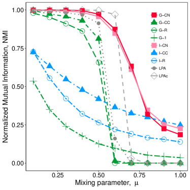
(a) NMI Scores

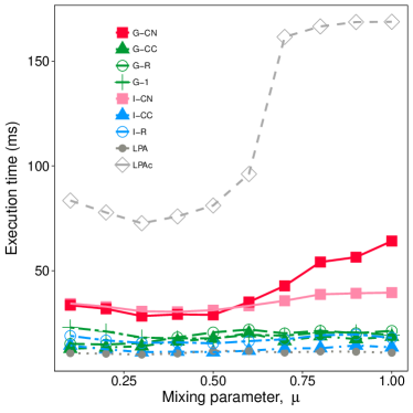
(b) Execution Times

Figure 4: (a) NMI scores and (b) execution times of our new algorithm with various benefit score candidates, and LPA and LPAc with $c=0.25$ on LFR benchmark network datasets. LFR parameters: $[N=1,000,\langle k\rangle=15,k_{max}=50,C_{min}=10,C_{max}=50]$. (Average of 100 realizations)

We observe that all the group-based benefit scores have better results than the individual ones. Even group-random value assignment, G-R, has good results.

Surprisingly, uniform benefit score using the group approach, G-1, has the worst performance among all. Although it is similar to the majority rule of labels in the LPA, it is not a good fit for our algorithm. As an exception among the individual ones, I-CN outperforms LPA.

Benefit scores based on common neighbors, both at individual and group level, i.e., I-CN and G-CN, produce better results in our tests. G-CN is slightly better than I-CN in terms of NMI values.

Both LPA and LPAc algorithms have good NMI values, but when $\mu>0.6$, their performances degrade while our algorithm still finds communities. LPAc performs better than LPA. However, when we look at the execution times of algorithms, LPAc has the worst performance. Its elapsed time is 2 to 3 times higher than our G-CN algorithm.

We conclude that using the number of common neighbors with the community-groups approach, namely G-CN, produces the best results in our algorithm. We use G-CN for the rest of the paper.

IV.2 Zachary karate club network

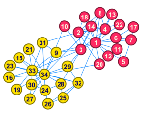
Figure 5: Zachary karate club: Identified communities by our G-CN algorithm

We run our algorithm on Zachary karate club network and compare the identified communities with the ground-truth. Our algorithm G-CN identifies two communities as seen in Fig. 5. Only the node 10 is misidentified by our algorithm. There is a tie-situation among the benefit scores exhibited to node 10 by its neighbors; so with random selection among alternatives our algorithm sometimes selects the wrong community. The community labels of all the other nodes are identified correctly with respect to ground-truth community structure.

Table 1: Large real-life networks with ground truth

Network	$|V|$	$|E|$	CC	# communities							NMI wrt GT						Execution time (ms)
				GT	G-CN	Inf	LPA	LPAc	Lvn	NM	G-CN	Inf	LPA	LPAc	Lvn	NM	G-CN	Inf	LPA	LPAc	Lvn	NM
European-email	1,005	16,064	0.40	42	23	38	3	20	25	28	0.14	0.62	0.13	0.31	0.54	0.46	146	133	32	704	69	187
DBLP	317,080	1,049,866	0.63	13,477	26,873	30,811	36,780	30,242	565	3,165	0.56	0.65	0.64	0.61	0.13	0.16	8,825	35,753	26,413	894,858	8,217	4,362,272
Amazon	334,863	925,872	0.40	75,149	33,395	35,139	24,045	30,908	248	1,474	0.57	0.60	0.54	0.57	0.11	0.11	7,552	43,253	30,931	997,088	8,017	1,422,590
YouTube	1,134,890	2,987,624	0.08	8,385	116,082	102,125	89,449	69,817	9,616	-	0.07	0.13	0.07	0.05	0.06	-	295,935	188,037	324,641	76,129,367	52,798	-

GT: Ground-truth	LPA : Label propagation algorithm Raghavan et al. (2007)
LPAc: Neighborhood-strength driven LPA Xie and Szymanski (2011)	G-CN: Our algorithm
Lvn: Louvain community detection algorithm Blondel et al. (2008)	Inf: Infomap algorithm Rosvall and Bergstrom (2007)
NM: Newman’s fast greedy algorithm Clauset et al. (2004)

IV.3 Large real-life networks

We run our G-CN  algorithm on large real-life networks with ground-truth communities, provided by SNAP Leskovec and Krevl (2014). For comparative analysis, Newman’s fast greedy algorithm (NM) Clauset et al. (2004), Infomap (Inf) Rosvall and Bergstrom (2007), Louvain (Lvn) Blondel et al. (2008), Label Propagation (LPA) Raghavan et al. (2007) and neighborhood-strength driven LPA (LPAc) Xie and Szymanski (2011) are also run on these networks. Newman’s algorithm is omitted for YouTube network due to its long execution time. The results are presented in Table 1.

There is no clear winner in Table 1, which is a good news for local algorithms. That is, although the local algorithms cannot see the global picture, they perform good enough.

The number of detected communities by G-CN, Infomap, LPA, and LPAc are close to each other and not far from the ground-truth. There are exceptions; on the YouTube network, all four detect too many communities. On European-email network with 42 ground-truth communities, LPA merges many communities together and detects only 3 communities while the other three do a better job. On DBLP and Amazon networks; both Louvain and Newman’s algorithm detect very few number of communities. Louvain has the best detection on YouTube network, while Newman’s algorithm experiences performance problems. Our G-CN algorithm performs well on most of the networks. However, it performs poorly on YouTube network, which has the smallest clustering coefficient of these four networks.

Considering NMI values of all six algorithms, it is possible that YouTube network may have subtle community structure. On this network, the best performing algorithm, Infomap, only gets NMI value of 0.13. On DBLP and Amazon networks; Infomap, LPA, LPAc and our algorithm obtain similar NMI values, and they are much better than Louvain and Newman’s algorithm. On European-email network, local algorithms like LPA, LPAc and ours are not good enough. It is possible that the network is not a good one for local approaches. On all of the networks, LPAc has highest execution times among the local algorithms. Its execution time on YouTube network is very high compared to our algorithm and LPA.

For all the real-life networks, we use the provided ground-truth community structure to evaluate the quality of partitions found by each algorithm. However, there is no single algorithm that performs good on all networks or there is not a single network on which some algorithms perform very good. This may be due to the fact that supposed ground-truth for these networks do not reflect the original ground-truth community structure or show different aspects of the network structure, as discussed in the work of Peel et al. Peel et al. (2017). For this reason, our test on real-life networks gives an idea about the relative performance of algorithms compared to each other on different networks; but does not lead to a conclusion on whether they perform well on these networks or not.

IV.4 Generated networks

We test our algorithm, G-CN, also on generated LFR networks of $1,000$ and $5,000$ nodes as reported in Fig. 6a and Fig. 6c, respectively. The same algorithms that we run on real-life networks are also used for comparative analysis on these networks. We also measure the execution times of the algorithms and report the results in Fig. 6b and in Fig. 6d. We present the details of the results on LFR networks of 5,000 nodes in Table 2. For each parameter set, we generate 100 LFR networks for a given $\mu$ and run algorithms on all these datasets and then average the results for each algorithm.

On LFR networks with 1,000 nodes, our G-CN algorithm is the best algorithm with Infomap when $0.1<\mu<0.5$. For $0.5<\mu<0.8$, our algorithm is in the second place after Infomap. When $\mu>0.7$, most of the algorithms tend to find a small number of communities while our algorithm still identifies a reasonable set of communities. LPA and LPAc find a single community that leads to the NMI value of $0$. Louvain and Newman’s algorithm also find very few number of communities on these networks.

Table 2: Generated LFR benchmark networks of 5,000 nodes

Network	$|V|$	$\mu$	$|E|$	CC	# communities							NMI wrt GT						Execution time (ms)
					GT	G-CN	Inf	LPA	LPAc	Lvn	NM	G-CN	Inf	LPA	LPAc	Lvn	NM	G-CN	Inf	LPA	LPAc	Lvn	NM
LFR-1	5,000	0.1	38,928	0.52	102	102	102	102	102	89	65	1.00	1.00	1.00	1.00	0.99	0.93	161	261	51	612	132	508
LFR-2	5,000	0.2	38,834	0.37	101	102	101	100	101	81	32	1.00	1.00	1.00	1.00	0.98	0.78	167	273	52	647	142	914
LFR-3	5,000	0.3	38,883	0.26	101	103	101	98	101	73	18	1.00	1.00	1.00	1.00	0.97	0.65	167	287	55	655	157	1,504
LFR-4	5,000	0.4	38,939	0.16	101	109	101	97	102	64	12	0.98	1.00	0.99	1.00	0.95	0.55	169	309	56	691	174	2,117
LFR-5	5,000	0.5	38,965	0.10	101	131	101	94	104	53	9	0.93	1.00	0.98	1.00	0.93	0.46	169	362	59	749	196	2,644
LFR-6	5,000	0.6	38,935	0.05	102	203	104	87	110	41	11	0.82	1.00	0.85	0.98	0.87	0.30	175	441	58	859	241	3,106
LFR-7	5,000	0.7	38,857	0.02	101	356	159	5	114	24	15	0.65	0.88	0.19	0.72	0.46	0.14	192	767	53	1,368	279	3,099
LFR-8	5,000	0.8	38,873	0.01	101	530	239	1	1	12	13	0.46	0.37	0.00	0.00	0.10	0.06	193	1,238	49	1,681	290	2,645
LFR-9	5,000	0.9	38,909	0.01	102	614	86	1	1	12	13	0.37	0.11	0.00	0.00	0.04	0.04	195	939	47	1,522	305	2,456
LFR-10	5,000	1.0	38,923	0.01	101	618	79	1	1	12	13	0.35	0.09	0.06	0.00	0.03	0.03	189	913	47	1,553	303	2,450

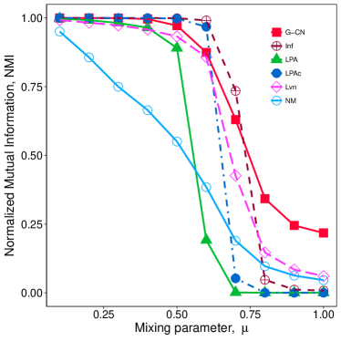
(a) NMI Scores

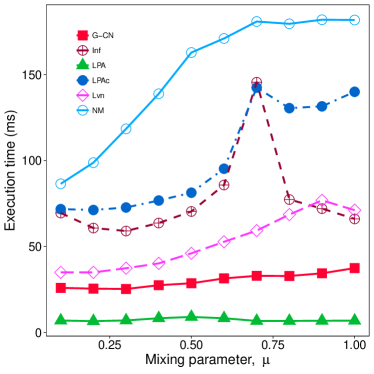
(b) Execution Times

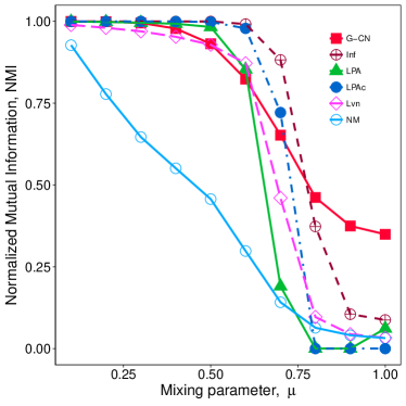
(c) NMI Scores

(d) Execution Times

Figure 6: Comparison of NMI and execution times of our method and known algorithms on LFR benchmark network datasets. (a) and (b) are for LFR network generated with $[N=1,000,\langle k\rangle=15,k_{max}=50,C_{min}=10,C_{max}=50]$. (c) and (d) are for LFR network generated with $[N=5,000,\langle k\rangle=15,k_{max}=75,C_{min}=20,C_{max}=100]$. (Average of 100 realizations)

The second set of test is performed on LFR networks of $5,000$ nodes. Infomap, LPA, and LPAc are successful in identifying communities when mixing parameter is low, however, their quality degrades with increasing mixing parameter. LPAc and LPA have slightly better results on the networks of $5,000$ nodes generated with $0.4<\mu<0.6$ compared to the previous set of networks of $1,000$ nodes. With increasing value of the $\mu$, performances of LPA and LPAc get worse and they tend to find a single community after $\mu>0.7$. Infomap has the similar tendency but has better results on LFR networks of $5,000$ nodes compared to previous set of networks of $1,000$ nodes. Newman’s algorithm and Louvain find a small number of communities; they tend to merge communities, which may lead to a resolution limit Fortunato and Barthélemy (2007).

Our G-CN algorithm identifies communities with high accuracy when $\mu$ is low. It is the only algorithm to identify communities when community identification becomes very hard, i.e., $\mu>0.75$. Its execution times are lower than most of the algorithms; only LPA has better execution times. However, considering the quality of identified communities and corresponding execution times, G-CN algorithm performs better than LPA. Newman’s algorithm and LPAc have the highest execution times on these networks.

V Conclusion

We propose a new local community detection algorithm, G-CN, which is based on identifying borderlines of communities using boundary nodes in the network. It is a local algorithm that is able to run on very large networks with low execution times. It can identify communities with high quality, regardless of the network size.

On the networks with subtle community structure, it outperforms other algorithms. On these networks; Infomap, LPA, and LPAc merge all the nodes into a single community. This is due to the heuristics of these algorithms, where they lose granular structures and fail to identify communities for certain kinds of networks. However, our approach keeps granular communities by focusing on the similarity of nodes even when it has many dissimilar neighbors but only a few similar ones. It does not force small communities to join to a giant component. Our algorithm performs successfully on generated networks with planted community structure, i.e., ground-truth is known. However, on real-life networks where ground-truth is created by using some meta-data, all of the algorithms in benchmark find different results. This may be due to the fact that meta-data does not reflect the actual ground-truth communities or meta-data shows different aspects of the network structure as discussed in the work of Peel et al. Peel et al. (2017).

With its local approach, G-CN is scalable and suitable for distributed and parallel processing (we have not implemented a parallel version for this paper). Community detection task can be split into separate subtasks on many computation devices (with the necessary piece of network data), which will enable real-time community detection on very large networks.

The source code of the algorithm is available at: https://github.com/murselTasginBoun/CDBN

References

- Onnela et al. (2007) J.-P. Onnela, J. Saramäki, J. Hyvönen, G. Szabó, D. Lazer, K. Kaski, J. Kertész, and A.-L. Barabási, Proceedings of the National Academy of Sciences 104, 7332 (2007).
- Newman (2001a) M. E. Newman, Proceedings of the National Academy of Sciences 98, 404 (2001a).
- Chen and Yuan (2006) J. Chen and B. Yuan, Bioinformatics 22, 2283 (2006).
- Girvan and Newman (2002) M. Girvan and M. E. Newman, Proceedings of the National Academy of Sciences 99, 7821 (2002).
- Newman (2004) M. E. Newman, Physical Review E 69, 066133 (2004).
- Clauset et al. (2004) A. Clauset, M. E. J. Newman, and C. Moore, Phys. Rev. E 70, 066111 (2004).
- Rosvall and Bergstrom (2007) M. Rosvall and C. T. Bergstrom, Proceedings of the National Academy of Sciences 104, 7327 (2007).
- Blondel et al. (2008) V. D. Blondel, J.-L. Guillaume, R. Lambiotte, and E. Lefebvre, Journal of Statistical Mechanics: Theory and Experiment 2008, P10008 (2008).
- Lancichinetti et al. (2011) A. Lancichinetti, F. Radicchi, J. J. Ramasco, and S. Fortunato, PloS One 6, e18961 (2011).
- De Meo et al. (2014) P. De Meo, E. Ferrara, G. Fiumara, and A. Provetti, Journal of Computer and System Sciences 80, 72 (2014).
- Raghavan et al. (2007) U. N. Raghavan, R. Albert, and S. Kumara, Physical Review E 76, 036106 (2007).
- Xie and Szymanski (2011) J. Xie and B. K. Szymanski, in Network Science Workshop (NSW), 2011 IEEE (IEEE, 2011), pp. 188–195.
- Gregory (2010) S. Gregory, New Journal of Physics 12, 103018 (2010).
- Eustace et al. (2015) J. Eustace, X. Wang, and Y. Cui, Physica A: Statistical Mechanics and its Applications 436, 665 (2015).
- Tasgin and Bingol (2018) M. Tasgin and H. O. Bingol, Physica A: Statistical Mechanics and its Applications 495, 126 (2018), ISSN 0378-4371.
- Fortunato (2010) S. Fortunato, Physics Reports 486, 75 (2010).
- Schaub et al. (2017) M. T. Schaub, J.-C. Delvenne, M. Rosvall, and R. Lambiotte, Applied Network Science 2, 4 (2017), ISSN 2364-8228.
- Radicchi et al. (2004) F. Radicchi, C. Castellano, F. Cecconi, V. Loreto, and D. Parisi, Proceedings of the National Academy of Sciences of the United States of America 101, 2658 (2004).
- Newman (2001b) M. E. Newman, Physical Review E 64, 025102 (2001b).
- Danon et al. (2005) L. Danon, A. Diaz-Guilera, J. Duch, and A. Arenas, Journal of Statistical Mechanics: Theory and Experiment 2005, P09008 (2005).
- Zachary (1977) W. W. Zachary, Journal of Anthropological Research 33, 452 (1977).
- Leskovec and Krevl (2014) J. Leskovec and A. Krevl, SNAP Datasets: Stanford large network dataset collection, http://snap.stanford.edu/data (2014).
- Peel et al. (2017) L. Peel, D. B. Larremore, and A. Clauset, Science Advances 3 (2017).
- Lancichinetti et al. (2008) A. Lancichinetti, S. Fortunato, and F. Radicchi, Physical Review E 78, 046110 (2008).
- Fortunato and Barthélemy (2007) S. Fortunato and M. Barthélemy, Proceedings of the National Academy of Sciences 104, 36 (2007).