Small-scale dynamos in simulations of stratified turbulent convection

Abstract

Small-scale dynamo action is often held responsible for the generation of quiet-Sun magnetic fields. We aim to determine the excitation conditions and saturation level of small-scale dynamos in non-rotating turbulent convection at low magnetic Prandtl numbers. We use high resolution direct numerical simulations of weakly stratified turbulent convection. We find that the critical magnetic Reynolds number for dynamo excitation increases as the magnetic Prandtl number is decreased, which might suggest that small-scale dynamo action is not automatically evident in bodies with small magnetic Prandtl numbers as the Sun. As a function of the magnetic Reynolds number (${\rm Rm}$), the growth rate of the dynamo is consistent with an ${\rm Rm}^{1/2}$ scaling. No evidence for a logarithmic increase of the growth rate with ${\rm Rm}$ is found.

1 Introduction

Magnetic fields are ubiquitous in astrophysical systems. These fields are in most cases thought to be generated by a dynamo process, involving either turbulent fluid motions or MHD-instabilities. In dynamo theory (e.g. Krause & Rädler 1980; Rüdiger & Hollerbach 2004; Brandenburg & Subramanian 2005; Brandenburg et al. 2012) a distinction is made between large-scale (LSD) and small-scale dynamos (SSD) where the former produce fields whose length scale is greater than the scale of fluid motions whereas in the latter the two are comparable. Also an LSD can produce small-scale magnetic fields through tangling, and the decay of active regions will similarly cause magnetic energy to cascade from larger to smaller scales, as is evidenced by the presence of a Kolmogorov-type energy spectrum in their proximity (Zhang et al. 2014, 2016).

Small-scale dynamos have been found in direct numerical simulations of various types of flows provided that the magnetic Reynolds number (${\rm Rm}$) exceeds a critical value (${\rm Rm}_{\rm c}$). However, in many astrophysical conditions molecular kinematic viscosity and magnetic diffusivity are vastly different implying that their ratio, which is the magnetic Prandtl number (${\rm Pm}$), is either very small or very large. For example, in the Sun ${\rm Pm}=10^{-3}\ldots 10^{-6}$ (e.g. Ossendrijver 2003). Numerical simulations of forced turbulence and other idealized flows indicate that ${\rm Rm}_{\rm c}$ increases as ${\rm Pm}$ is decreased (Ponty et al. 2004; Schekochihin et al. 2004, 2005, 2007; Iskakov et al. 2007). Theoretical studies indicate a similar trend with an asymptotic value for ${\rm Rm}_{\rm c}$ when ${\rm Pm}\rightarrow 0$ (Rogachevskii & Kleeorin 1997). The work of Iskakov et al. (2007) suggests that there is a value of ${\rm Pm}$ of around $0.1$ where ${\rm Rm}_{\rm c}$ is largest and that it decreases again somewhat at even smaller values of ${\rm Pm}$. In the nonlinear regime, however, no significant drop in the magnetic energy is seen as ${\rm Pm}$ is decreased to and below $0.1$ (Brandenburg 2011). More recently, Subramanian & Brandenburg (2014) found that the drop in the value of ${\rm Rm}_{\rm c}$ may have been exaggerated by having used a forcing wavenumber that was too close to the minimal wavenumber of the computational domain.

Simulations of turbulent convection have also been able to produce SSDs (e.g. Meneguzzi & Pouquet 1989; Nordlund et al. 1992; Brandenburg et al. 1996; Cattaneo 1999; Pietarila Graham et al. 2010; Favier & Bushby 2012; Hotta et al. 2015). Such small-scale magnetic fields may explain the network of magnetic fields in the Sun, which are independent of the solar cycle (Buehler et al. 2013; Stenflo 2014; Rempel 2014); see Brun & Browning (2017) and Borrero et al. (2017) for reviews. However, even the expected independence of the cycle does not go without controversy (Faurobert & Ricort 2015; Utz et al. 2016). In fact, Jin et al. (2011) found evidence for an anticorrelation of small-scale fields with the solar cycle. This could potentially be explained by the interaction of the SSD with superequipartition large-scale fields from the global dynamo; see Karak & Brandenburg (2016). Small-scale magnetic fields may also play a role in heating the solar corona; see Amari et al. (2015) for recent work in that direction.

Small-scale dynamo-produced magnetic fields have been invoked (Hotta et al. 2015, 2016; Bekki et al. 2017) to explain the convective conundrum of the low levels of observed turbulent velocities compared to contemporary simulations (e.g. Gizon & Birch 2012; Miesch et al. 2012). Subsequent work of Karak et al. (2018), who studied cases of large thermal Prandtl numbers conjectured to be due to the magnetic suppression of thermal diffusion, does however cast some doubt on this idea.

Returning to the problem of magnetic Prandtl numbers, Thaler & Spruit (2015) studied the case ${\rm Pm}\geq 1$ from local solar surface convection simulations and found that the SSD ceases to exist already for ${\rm Pm}=1$. However, this is mainly a shortcoming of low resolution. Global and semi-global simulations of solar and stellar magnetism have also recently reached parameter regimes where SSDs are obtained (Hotta et al. 2016; Käpylä et al. 2017). These models suggest that the vigorous small-scale magnetism has profound repercussions for the LSD and differential rotation. However, due to resolution requirements the global simulations are limited to magnetic Prandtl numbers of the order of unity or greater.

In the present paper, we therefore study high-resolution simulations of convection-driven SSDs in the case of small values of ${\rm Pm}$ by means of local models capturing more turbulent regimes. This regime was already addressed in an early paper by Cattaneo (2003), but no details regarding the dependence of the growth rates and saturation values of the magnetic field are available.

2 The model

Our numerical model is the same as that of Käpylä et al. (2010) but without imposed shear or rotation. We use a Cartesian domain with dimensions $L_{x}=L_{y}=5d$ and $L_{z}=d$ with $0<z<d$, where $d$ is the depth of the layer.

2.1 Basic equations and boundary conditions

We solve the set of equations of magnetohydrodynamics

$$\frac{\partial\bm{A}}{\partial t} = \bm{U}\times\bm{B}-\eta\mu_{0}\bm{J},$$ (1)

$$\frac{D\ln\rho}{Dt} = -\bm{\nabla}\cdot\bm{U},$$ (2)

$$\frac{D\bm{U}}{Dt} = {\bm{g}}-\frac{1}{\rho}\left[{\bm{\nabla}}p+\bm{J}\times{\bm{B}}+\bm{\nabla}\cdot(2\nu\rho\mbox{\boldmath${\sf S}$})\right],$$ (3)

$$T\frac{Ds}{Dt}\! = \!\frac{1}{\rho}\left(\mu_{0}\eta\bm{J}^{2}-\bm{\nabla}\cdot{\bm{F}}^{\rm rad}\right)+2\nu\mbox{\boldmath${\sf S}$}^{2},$$ (4)

where $D/Dt=\partial/\partial t+\bm{U}\cdot\bm{\nabla}$ is the advective time derivative, $\bm{A}$ is the magnetic vector potential, $\bm{B}=\bm{\nabla}\times\bm{A}$ is the magnetic field, and $\bm{J}=\mu_{0}^{-1}\bm{\nabla}\times\bm{B}$ is the current density, $\mu_{0}$ is the vacuum permeability, $\eta$ and $\nu$ are the magnetic diffusivity and kinematic viscosity, respectively, ${\bm{F}}^{\rm rad}=-K\mbox{\boldmath$\nabla$}{}T$ is the radiative flux, $K$ is the (constant) heat conductivity, $\rho$ is the density, $\bm{U}$ is the velocity, $p$ is the pressure and $s$ the specific entropy with $Ds=c_{\rm V}D\ln p-c_{\rm P}D\ln\rho$, and $\bm{g}=-g\hat{\bm{z}}$ is the gravitational acceleration. The fluid obeys an ideal gas law $p=\rho e(\gamma-1)$, where $p$ and $e$ are the pressure and internal energy, respectively, and $\gamma=c_{\rm P}/c_{\rm V}=5/3$ is the ratio of specific heats at constant pressure and volume, respectively. The specific internal energy per unit mass is related to the temperature via $e=c_{\rm V}T$. The rate of strain tensor ${\sf S}$ is given by

$${\sf S}_{ij}={\textstyle{1\over 2}}(U_{i,j}+U_{j,i})-{\textstyle{1\over 3}}\delta_{ij}\bm{\nabla}\cdot\bm{U}.$$ (5)

In order to exclude complications due to overshooting and compressibility, we employ a weak stratification: the density difference between the top and bottom of the domain is twenty per cent and the average Mach number, ${\rm Ma}=u_{\rm rms}/\sqrt{dg}$, is always less than 0.1. The stratification in the associated hydrostatic initial state can be described by a polytrope with index $m=1$. The stratification is controlled by the normalized pressure scale height at the surface

$$\xi_{0}=\frac{(c_{\rm P}-c_{\rm V})T_{1}}{gd},$$ (6)

where $T_{1}$ is the temperature at the surface ($z=d$). In our current simulations we use $\xi_{0}=2.15$.

The horizontal boundary conditions are periodic. We keep the temperature fixed at the top and bottom boundaries. For the velocity we apply impenetrable, stress-free conditions according to

$$\partial_{z}U_{x}=\partial_{z}U_{y}=U_{z}=0.$$ (7)

For the magnetic field we use vertical field conditions

$$B_{x}=B_{y}=0.$$ (8)

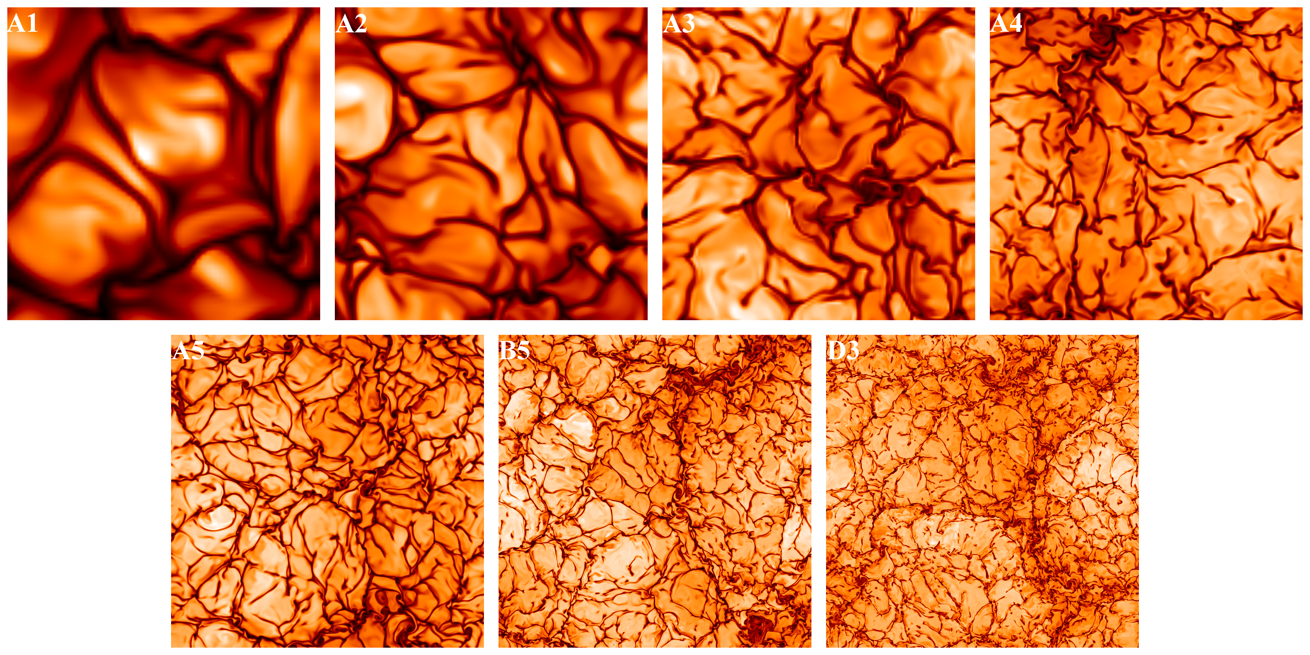
Figure 1: Upper row: specific entropy $s/c_{\rm P}$ near the surface $z/d=0.98$ for ${\rm Re}={\rm Pe}=$ 23, 54, 101, and 193. Lower row: ${\rm Re}={\rm Pe}=$ 354, 666, and 1057.

2.2 Units, nondimensional quantities, and parameters

The units of length, time, velocity, density, specific entropy, and magnetic field are then

$$[x]=d\;,\;\;[t]=\sqrt{d/g}\;,\;\;[U]=\sqrt{dg}\;,\;\;$$

$$[\rho]=\rho_{0}\;,\;\;[s]=c_{\rm P}\;,\;\;[B]=\sqrt{dg\rho_{0}\mu_{0}}\;,$$ (9)

where $\rho_{0}$ is the density of the initial state at $z_{\rm m}={\textstyle{1\over 2}}d$. The simulations are controlled by the following dimensionless parameters: thermal and magnetic diffusion in comparison to viscosity are measured by the Prandtl numbers

$$\Pr=\frac{\nu}{\chi_{0}},\quad{\rm Pm}=\frac{\nu}{\eta},$$ (10)

where $\chi_{0}=K/(c_{\rm P}\rho_{0})$ is the reference value of the thermal diffusion coefficient, measured in the middle of the layer, $z_{\rm m}$, in the non-convecting initial state. The efficiency of convection is measured by the Rayleigh number

$${\rm Ra}=\frac{gd^{4}}{\nu\chi_{0}}\left(-\frac{1}{c_{\rm P}}\frac{{\rm d}s}{{\rm d}z}\right)_{z_{\rm m}},$$ (11)

again determined from the initial non-convecting state at $z_{\rm m}$. The entropy gradient can be presented as

$$\left(-\frac{1}{c_{\rm P}}\frac{{\rm d}s}{{\rm d}z}\right)_{z_{\rm m}}=\frac{\nabla-\nabla_{\rm ad}}{H_{\rm P}},$$ (12)

where $\nabla=(\partial\ln T/\partial\ln p)_{z_{\rm m}}$ and $\nabla_{\rm ad}=1-1/\gamma$ are the actual and adiabatic double-logarithmic temperature gradients and $H_{\rm P}$ is the pressure scale height at $z=z_{\rm m}$.

The effects of viscosity and magnetic diffusion are quantified respectively by the fluid and magnetic Reynolds numbers

$${\rm Re}=\frac{u_{\rm rms}}{\nu k_{\rm f}},\quad{\rm Rm}=\frac{u_{\rm rms}}{\eta k_{\rm f}}={\rm Pm}\,{\rm Re},$$ (13)

where $u_{\rm rms}$ is the root mean square (rms) value of the velocity, and $k_{\rm f}=2\pi/d$ is the wavenumber corresponding to the depth of the layer. Furthermore, we define the P$\acute{\rm e}$clet number as

$${\rm Pe}=\frac{u_{\rm rms}}{\chi_{0}k_{\rm f}}={\rm Pr}\,{\rm Re}.$$ (14)

Except for the simulations of Section 3.5, where ${\rm Pr}={\rm Pm}$ is varied, we use in all other simulations ${\rm Pr}=1$ and thus ${\rm Pe}={\rm Re}$.

Error estimates are obtained by dividing the time series into three equally long parts. The largest deviation of the average for each of the three parts from that over the full time series is taken to represent the error.

The simulations were performed using the Pencil Code, which uses sixth-order explicit finite differences in space and a third-order accurate time stepping method. We use resolutions ranging from $64^{3}$ to $1024^{3}$.

Table 1: Summary of weak field runs for $\Pr=1$.

$$\begin{array}[]{p{0.07\linewidth}cccccrrcc}\hline\cr\vskip 3.0pt plus 1.0pt minus 1.0pt\cr Run&{\rm Pm}&{\rm Ra}[10^{6}]&{\rm Ma}&{\rm Re}&{\rm Rm}&\tilde{\lambda}[10^{-4}]&\delta\tilde{\lambda}[10^{-4}]&$grid$\\ \hline\cr A1&1&0.17&0.073&23&23&-52&47&64^{3}\\ A2&1&1.0&0.068&54&54&62&18&128^{3}\\ A3&1&4.2&0.064&101&101&162&20&128^{3}\\ A4&1&17&0.061&193&193&273&7&256^{3}\\ A5&1&67&0.056&354&354&453&2&512^{3}\\ \hline\cr B1&0.5&1.0&0.069&54&27&-128&24&128^{3}\\ B2&0.5&4.2&0.064&102&51&-27&12&128^{3}\\ B3&0.5&17&0.060&191&95&44&11&256^{3}\\ B4&0.5&67&0.056&360&180&155&18&512^{3}\\ B5&0.5&267&0.052&666&333&357&17&1024^{3}\\ \hline\cr C1&0.25&17&0.060&190&47&-144&22&256^{3}\\ C2&0.25&67&0.056&358&90&-35&28&512^{3}\\ \hline\cr D1&0.1&67&0.057&360&36&-237&56&512^{3}\\ D2&0.1&267&0.052&664&65&-139&77&1024^{3}\\ D3&0.1&740&0.050&1057&106&-10&94&1024^{3}\\ \hline\cr\end{array}$$

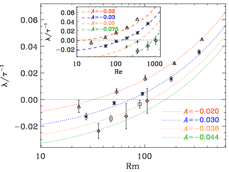
Figure 2: Growth rate $\lambda$ of the rms magnetic field normalized by the inverse convective turnover time $\tau^{-1}=u_{\rm rms}k_{\rm f}$ as a function of the magnetic Reynolds number ${\rm Rm}$. The different symbols denote runs with ${\rm Pm}=1$ (triangles), ${\rm Pm}=0.5$ (stars), ${\rm Pm}=0.25$ (squares), and ${\rm Pm}=0.1$ (diamonds). The horizontal dotted line denotes marginal stability. The red, blue, orange, and green dotted lines are curves proportional to ${\rm Rm}^{1/2}$; see Equation (16) for different values of $A$ and $B=3.5\cdot 10^{-3}$ is fixed. The inset shows the normalized growth rates for the same data as functions of ${\rm Re}$. The dashed lines are proportional to ${\rm Re}^{1/2}$ according to a relation analogous to Equation (16) with $B=2.5\cdot 10^{-3}$ and values of $A$ indicated in the legend.

3 Results

3.1 Description of the runs

We perform four sets of runs where we keep the magnetic Prandtl number fixed and vary ${\rm Re}$ and ${\rm Rm}$; see Table 1. The lower resolution ($64^{3}$, $128^{3}$, and $256^{3}$) runs were started from a non-convecting state described in the previous section, whereas runs at $512^{3}$ and $1024^{3}$ were remeshed from saturated snapshots at lower resolutions; see Figure 1 for visualizations of specific entropy near the surface of the domain. After the convection has reached a statistically saturated state we introduce a weak random magnetic field of the order of $10^{-6}B_{\rm eq}$, where $B_{\rm eq}$ is the equipartition field strength with $B_{\rm eq}^{2}=\langle\mu_{0}\rho\bm{u}^{2}\rangle$. We refer to these runs as weak field models and perform the data analysis in regimes where the magnetic fields remains dynamically unimportant. After an initial transient, the growth rate of the total rms magnetic field is measured as

$$\lambda=\langle d\ln B_{\rm rms}/dt\rangle_{t},$$ (15)

where $\langle\cdots\rangle_{t}$ denotes time averaging. In the runs where the dynamo is clearly above or below critical, a short time series (few tens of turnover times) is sufficient to measure a statistically significant value of $\lambda$. The runs near the excitation threshold need to be run significantly longer (hundreds of turnover times). For the highest resolution runs at low ${\rm Pm}$ this is not feasible due to the computational cost and thus the error bars for these runs are typically significantly larger than in the low resolution or ${\rm Pm}=1$ runs.

3.2 Growth rate in the kinematic regime

Figure 2 shows the growth rate of the magnetic field as a function of ${\rm Rm}$ for the four magnetic Prandtl numbers explored in the current study. For reference, we plot curves of the form

$$\gamma/\tau^{-1}\equiv\tilde{\gamma}=A+B\,{\rm Rm}^{1/2},$$ (16)

where the value of the constant $A$ changes as the magnetic Prandtl number is changed. Furthermore, $B=3.5\cdot 10^{-3}$ for all values of ${\rm Pm}$. The parameter $A$ is negative, so the solutions will always decay for small values of ${\rm Rm}$, but they increase with increasing values of ${\rm Pm}$; see Figure 2.

We find that the normalized growth rate for a given ${\rm Rm}$ decreases as ${\rm Pm}$ is decreased. Surprisingly, $\tilde{\lambda}$ appears to follow a ${\rm Rm}^{1/2}$ trend for each value of ${\rm Pm}$ – even in the cases when an SSD is not excited. Such a dependence is predicted by theory for high ${\rm Rm}$, i.e. far away from excitation (Kleeorin & Rogachevskii 2012). However, given the relatively large error bars, the ${\rm Rm}^{1/2}$ scaling near the excitation threshold can at this point only be suggestive and far from definitive. Indeed, analytic theory yields a different scaling in this regime (Kleeorin & Rogachevskii 2012).

In the low-${\rm Pm}$ regime, the growth rate of the magnetic field due to the SSD is expected to scale with the 1/2 power of the fluid Reynolds number. We find that our simulation data is consistent with this for values of ${\rm Pm}$ of 0.5 and smaller; see the inset to Figure 2.

3.3 Dependence on the box size

The dependence of the growth rate of the convection-driven SSD on the horizontal size of the domain and the presence of mesogranulation has been discussed in a recent paper by Bushby et al. (2012). To address this issue, we show in Figure 3 the growth rate of the magnetic field as a function of the horizontal box size for magnetic Prandtl number unity. Deviations from the constant trend are found for $L_{\rm H}/d=1.25$. For $L_{\rm H}/d=0.5$, no dynamo action is found. Our standard box size of $L_{\rm H}/d=5$ is thus adequate and does not seem to suffer from the issues raised by Bushby et al. (2012). This is in spite of the fact that the flow is dominated by a single convection cell filling the whole domain, which is clear even by visual inspection of Figure 1.

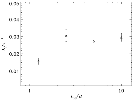
Figure 3: Growth rate $\lambda$ of the rms magnetic field normalized by the inverse convective turnover time $\tau^{-1}=u_{\rm rms}k_{\rm f}$ as a function of the horizontal box size for ${\rm Pm}=1$.

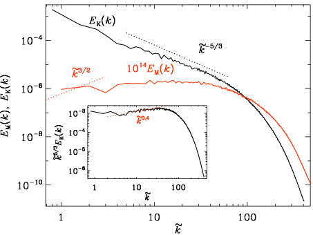
Figure 4: Power spectra of velocity and magnetic field as functions of $\tilde{k}=k/k_{1}$ near the top of the domain from Run B5. $E_{\rm M}$ has been multiplied by $10^{14}$ for visualization purposes. The dotted line show a $k^{-5/3}$ scaling for reference. The inset shows the velocity power spectrum compensated by $k^{5/3}$.

3.4 Energy spectra

In Figure 4 we show the kinetic and magnetic energy spectra, $E_{\rm K}$ and $E_{\rm M}$, respectively, for Run B5 during the kinematic phase of the dynamo for ${\rm Pm}=0.25$ and ${\rm Rm}=654$. The kinetic energy spectrum shows a clear $k^{-5/3}$ spectrum along with a slightly shallower slope near the dissipative cutoff. This is the bottleneck effect (Falkovich 1994), which has been held responsible for causing the increase of ${\rm Rm}_{\rm c}$ near ${\rm Pm}=0.1$, because then the peak of the magnetic energy lies fully within the inertial range of the kinetic energy spectrum (Boldyrev & Cattaneo 2004). The magnetic energy spectrum, on the other hand, is significantly shallower than the $k^{3/2}$ spectrum expected from the work of Kazantsev (1968), which has been confirmed in many in several numerical simulations of kinematic dynamo action in forced turbulence (Haugen et al. 2004; Schekochihin et al. 2004) and supernova-driven turbulence (Balsara et al. 2004). The spectra shown in Figure 4 were taken from a run where the magnetic field has grown only by a factor of a few and it is possible that the 3/2 scaling has not had enough time to develop yet. However, the flow exhibits a long-lived large-scale component, manifested by the peak at $\tilde{k}=1$, which is not present in simpler forced turbulence simulations. Such flows may contribute to the relatively high magnetic power at large scales. In that case, the lack of a $k^{3/2}$ spectrum in the kinematic regime would have a physical origin. These aspects will be explored further elsewhere.

Table 2: Summary of strong field runs.

$$\begin{array}[]{p{0.07\linewidth}ccccrrcc}\hline\cr\vskip 3.0pt plus 1.0pt minus 1.0pt\cr Run&{\rm Pm}&\Pr&{\rm Ra}[10^{6}]&{\rm Re}&{\rm Rm}&{\rm Ma}&\tilde{B}_{\rm rms}&$grid$\\ \hline\cr S1&1&1&17&169&169&0.053&0.0130&256^{3}\\ S2&0.5&0.5&33&361&180&0.057&0.0126&256^{3}\\ S3&0.25&0.25&67&760&190&0.060&0.0110&256^{3}\\ S4&0.1&0.1&167&2118&212&0.067&-&512^{3}\\ \hline\cr\end{array}$$

3.5 Saturation level

Another set of simulations was made to study the saturation level of the magnetic fields produced by the SSD; see Table 2. We refer to these runs as strong field models. These runs were either run to full saturation from the initial conditions described in Section 2 (Run S1) or continued from a saturated snapshot of an earlier run (S2, S3, or S4). At each step, the kinematic viscosity is lowered to decrease ${\rm Pm}$ with the aim of avoiding the long kinematic stage of the dynamo. Another possible advantage of this procedure is that the SSD has been shown to operate in the nonlinear regime at an ${\rm Rm}$ value that would be subcritical in the kinematic case (Brandenburg 2011). While this procedure works for Runs S2 and S3, in Run S4 with ${\rm Pm}=0.1$ where ${\rm Rm}=212$ and ${\rm Re}=2118$ the magnetic field is not sustained, however.

Figure 5 shows the saturation field strength for Runs S1 to S3 with ${\rm Pm}=0.25\ldots 1$. Here the magnetic Reynolds number varies from 169 to 190 due to increasing $u_{\rm rms}$ when ${\rm Pm}$ decreases. Contrary to the results for forced turbulence, where the rms magnetic field was found to decrease by no more than a factor of two as ${\rm Pm}$ was decreased from unity to $0.01$ (Brandenburg 2011), we seem to find here a somewhat stronger dependence of the saturation field strength on the value of ${\rm Pm}$ and thus on ${\rm Re}$. The current results suggest a scaling with ${\rm Re}$ with a power that is close to $-1/3$. However, one has to realize that for the run with the largest value of ${\rm Re}$ and ${\rm Pm}=0.25$, we used a resolution of $256^{3}$ which may be too low to resolve the flow at ${\rm Re}=760$.

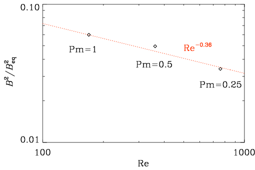
Figure 5: Saturation field strength for Runs S1 to S3 with ${\rm Pm}=1\ldots 0.25$ (${\rm Rm}=169\ldots 190$) as a function of the fluid Reynolds number.

4 Conclusions

Our work has confirmed that in turbulent convection at low values of ${\rm Pm}$, the value of ${\rm Rm}_{\rm c}$ increases with decreasing ${\rm Pm}$. This effect may well be connected with the bottleneck effect seen in the kinetic energy spectrum. The saturated field strength, however, is found to show a somewhat stronger dependence on ${\rm Pm}$ than in the case of forced turbulence.

Both for small values of ${\rm Pm}$ and for ${\rm Pm}$ of unity, we find that the kinematic growth rate increases proportional to ${\rm Rm}^{1/2}$. In particular, there is no evidence for a logarithmic dependence. A similar dependence on ${\rm Rm}$ has previously been seen in forced turbulence; see Haugen et al. (2004), for example.

Interestingly, however, in the kinematic regime, the magnetic energy spectrum is significantly shallower than the $k^{3/2}$ spectrum expected for an SSD (Kazantsev 1968). This is also quite different from the case of forced turbulence, where a clear $k^{3/2}$ spectrum is found during the kinematic growth phase. In other words, the current kinematic convection-driven dynamo show a tendency of producing larger-scale magnetic fields than in forced turbulence. This is possibly caused by a persistent large-scale velocity pattern which is a robust feature in the current simulations.