Points on nodal lines with given direction

Abstract.

We study of the directional distribution function of nodal lines for eigenfunctions of the Laplacian on a planar domain. This quantity counts the number of points where the normal to the nodal line points in a given direction. We give upper bounds for the flat torus, and compute the expected number for arithmetic random waves.

1. Introduction

1.1. Nodal directions

One of the more intriguing characteristics of a Laplace eigenfunction on a planar domain is its nodal set. Much progress has been achieved in understanding its length, notably the work of Donnelly and Fefferman [4], and the recent breakthrough by Logunov and Mallinikova [9, 8, 7], and several researchers have tried to understand the number of nodal domains (the connected components of the complement of the nodal set), starting with Courant’s upper bound on that number, see [2] for the latest result. In this note, we propose to study a different quantity, the directional distribution, measuring an aspect of the curvature of nodal lines.

Let $\Omega$ be a planar domain, with piecewise smooth boundary, and let $f$ be an eigenfunction of the Dirichlet Laplacian, with eigenvalue $E$: $-\Delta f=Ef$. Given a direction $\zeta\in S^{1}$, let $N_{\zeta}(f)$ be the number of points $x$ on the nodal line $\{x\in\Omega:f(x)=0\}$ with normal pointing in the direction $\pm\zeta$:

(1.1) $$N_{\zeta}(f)=\#\left\{x\in\Omega:\>f(x)=0,\frac{\nabla f(x)}{\|\nabla f(x)\|}=\pm\zeta\right\}.$$

In particular (1.1) requires that $\nabla f(x)\neq 0$, i.e. $x$ is a non-singular point of the nodal line.

In a few separable cases, such as an irrational rectangle, or the disk, one can explicitly compute $N_{\zeta}(f)$: For the irrational rectangle, the nodal line is a grid and $N_{\zeta}(f)=0,\infty$, while for the disk the nodal line is a union of diameters and circles, and we find $N_{\zeta}(f)\ll\sqrt{E}$ except for $O(\sqrt{E})$ choices of $\zeta$, when $N_{\zeta}(f)=\infty$, see Appendix A. However, in most cases one cannot explicitly compute $N_{\zeta}(f)$. The following heuristic suggests that generically the order of magnitude of $N_{\zeta}(f)$ is about $E$: We expect a “typical” eigenfunction to have an order of magnitude of $E$ nodal domains [13], and looking at several plots of nodal portraits such as Figure 1 would lead us to believe that many of the nodal domains are ovals, or at least have a controlled geometry, with $O(1)$ points per nodal domain with normal parallel to any given direction. Therefore we are led to expect that the total number of points on the nodal line with normal parallel to $\pm\zeta$ should be about $E$ (if it is finite).

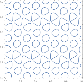
Figure 1. The nodal line of the toral eigenfunction

$$\sin(2\pi(8x-y))+\sin(2\pi(4x+7y))+\cos(2\pi(4x-7y)).$$

A significant proportion of its components are ovals.

To try and validate this heuristic, we study $N_{\zeta}(f)$ on the standard flat torus $\mathbb{T}=\mathbb{R}^{2}/\mathbb{Z}^{2}$ (equivalently taking $\Omega$ to be the square, and imposing periodic, rather than Dirichlet, boundary conditions), for both random and deterministic eigenfunctions. We prove deterministic upper bounds, and compute the expected value of $N_{\zeta}$ for “arithmetic random waves” described below.

1.2. A deterministic upper bound

We want to establish individual upper bounds on $N_{\zeta}(f)$. Strictly speaking, this is not possible, since there are cases where $N_{\zeta}(f)=\infty$. For instance, the nodal set of the eigenfunctions $f(x,y)=\sin(2\pi mx)\sin(2\pi ny)$ ($m,n\geq 1$) is a union of straight lines with $N_{\zeta}(f)=0$ unless $\zeta=\pm(1,0),\pm(0,1)$ in which case $N_{\zeta}(f)=\infty$. More generally, one can construct toral eigenfunctions $f$ so that their nodal lines contain a closed geodesic, but also curved components, see Figure 2 where we display the eigenfunction

$$\begin{split}f(x,y)&=2\Big{(}\sin 8x\sin y+\sin 7x\sin 4y+\sin x\sin 8y+\sin 4x\sin 7y\Big{)}\\ &=4\sin(x)\sin(y)\Big{(}\cos x+\cos y\Big{)}h(x,y)\end{split}$$

where

(1.2) $$h(x,y)=2\cos(3x-5y)-2\cos(2x-4y)-2\cos(4x-4y)+4\cos(x-3y)+4\cos(3x-3y)\\ +2\cos(5x-3y)-4\cos(2x-2y)-2\cos(4x-2y)+6\cos(x-y)+4\cos(3x-y)+6\cos(x+y)+4\cos(3x+y)\\ -4\cos(2x+2y)-2\cos(4x+2y)+4\cos(x+3y)+4\cos(3x+3y)+2\cos(5x+3y)-2\cos(2x+4y)\\ -2\cos(4x+4y)+2\cos(3x+5y)-4\cos(2x)+2\cos(6x)-4\cos(2y)+2\cos(6y)-2.$$

Theorem 1.2 below asserts an upper bound for $N_{\zeta}(f)$ with the only exceptions being when the nodal line contains a closed geodesic. It will follow as a particular case of a structure result on the set

(1.3) $$\mathcal{A}_{\zeta}(f)=\left\{x\in\Omega:\>f(x)=0,\langle\nabla f(x),\zeta^{\perp}\rangle=0\right\}$$

of “nodal directional points”, i.e. the set of nodal points where $\nabla f$ is orthogonal to $\zeta^{\perp}$ (thus co-linear to $\zeta$). Note that, by the definition, in addition to the set on the r.h.s. of (1.1), $\mathcal{A}_{\zeta}(f)$ contains all the singular nodal points of $f^{-1}(0)$, and could also contain certain closed geodesics in direction orthogonal to $\zeta$, as we shall see below. To state Theorem 1.2 we introduce the (standard) notion of “height” for a rational vector.

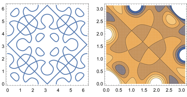
Figure 2. Left: nodal set of the eigenfunction $f(x,y)=2\Big{(}\sin 8x\sin y+\sin 7x\sin 4y+\sin x\sin 8y+\sin 4x\sin 7y\Big{)}=4\sin(x)\sin(y)\Big{(}\cos x+\cos y\Big{)}h(x,y)$ for the trigonometric polynomial $h(x,y)$ in (1.2), on the full square $[0,2\pi]\times[0,2\pi]$. Note the lines $x,y\in\pi\mathbb{Z}$, $x\pm y\in\pi(1+2\mathbb{Z})$. The scaled function $f(x/2\pi,y/2\pi)$ is a toral eigenfunction. Right: Contours of $h(x,y)$ on the square $[0,\pi]\times[0,\pi]$.

Notation 1.1 (Height of a rational vector).

1. A rational direction $\zeta\in\mathcal{S}^{1}$ is one which is a multiple of an integer vector. Note that $\zeta$ is rational if and only if the orthogonal direction $\zeta^{\perp}$ is rational.

2. For a rational vector $\zeta\in\mathcal{S}^{1}$ we denote its height by $h(\zeta)=\max(|k_{1}|,|k_{2}|)$ where $(k_{1},k_{2})$ is a primitive integer vector (unique up to sign) in the direction of $\zeta$:

   $$\zeta=\pm\frac{(k_{1},k_{2})}{\sqrt{k_{1}^{2}+k_{2}^{2}}}\;.$$

   Note that $h(\zeta)=h(\zeta^{\perp})$.

Theorem 1.2.

Let $\zeta\in\mathcal{S}^{1}$ be a direction, and $f$ be a toral eigenfunction: $-\Delta f=Ef$ for some $E>0$.

1. If $\zeta$ is rational, then the set $\mathcal{A}_{\zeta}(f)$ consists of at most

   $$\frac{\sqrt{E}}{\pi h(\zeta)}$$

   closed geodesics orthogonal to $\zeta$, at most $\frac{2}{\pi^{2}}\cdot E$ nonsingular points not lying on the geodesics, and possibly, singular points of the nodal set.

2. If $\zeta$ is not rational, then the set $\mathcal{A}_{\zeta}(f)$ consists of at most $\frac{2}{\pi^{2}}\cdot E$ nonsingular points, and possibly, singular points of the nodal set.

3. In particular, if $\mathcal{A}_{\zeta}(f)$ does not contain a closed geodesic, then

   $$N_{\zeta}(f)\leq\frac{2}{\pi^{2}}\cdot E.$$

The proof of Theorem 1.2, given in section 2 below, is sufficiently robust to apply verbatim to the more general family of trigonometric polynomials on $\mathbb{T}^{2}$ of degree $\leq\sqrt{E}$. We note that it is possible to construct Laplace eigenfunctions $f$ of arbitrarily high eigenvalues and $\zeta\in\mathcal{S}^{1}$ such that $N_{\zeta}(f)=0$ vanishes, so that a general lower bound for $N_{\zeta}(f)$ cannot exist. For example,

$$f(x,y)=2\cos(2\pi\cdot mx)+\cos(2\pi\cdot my)$$

has eigenvalue $E=4\pi^{2}m^{2}$ and satisfies $N_{\zeta}(f)=0$ for $\zeta=e^{i\theta}$ with $\theta$ near $\pi/2$, see Figure 3.

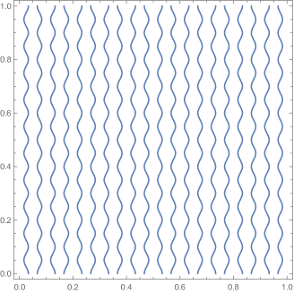
Figure 3. The nodal line of $f(x,y)=2\cos(2\pi\cdot 10x)+\cos(2\pi\cdot 10y)$. For the choice $\zeta=e^{i\pi/2}$ we have $N_{\zeta}(f)=0$.

1.3. Expected number for arithmetic random waves

A better understanding of several properties of nodal lines is obtained if one studies random eigenfunctions. In 1962, Swerling [18] studied statistical properties of contour lines of a general class of planar Gaussian processes, and gave a non-rigorous computation of the expected value of $N_{\zeta}$ for general contour lines, using the result to bound the number of closed connected components of contour lines. We will compute the expected value of $N_{\zeta}$ for “arithmetic random waves” [15, 17]. These are random eigenfunctions on the torus,

(1.4) $$f(x)=f_{n}(x)=\sum\limits_{\lambda\in\mathcal{E}_{n}}c_{\lambda}e(\langle\lambda,x\rangle),$$

where $e(z)=e^{2\pi iz}$ and

(1.5) $$\mathcal{E}_{n}=\{\lambda=(\lambda_{1},\lambda_{2})\in\mathbb{Z}^{2}:\>\|\lambda\|^{2}=n\}$$

is the set of all representations of the integer $n=\lambda_{1}^{2}+\lambda_{2}^{2}$ as a sum of two integer squares, and $c_{\lambda}$ are standard Gaussian random variables, identically distributed and independent save for the constraint

(1.6) $$c_{-\lambda}=\overline{c_{\lambda}}\;,$$

making $f_{n}$ real valued eigenfunctions of the Laplacian with eigenvalue

(1.7) $$E=4\pi^{2}n$$

for every choice of the coefficients $\{c_{\lambda}\}_{\lambda\in\mathcal{E}_{\lambda}}$ (i.e. for every sample point).

Equivalently $f_{n}:\mathbb{T}^{2}\rightarrow\mathbb{R}$ is a centred Gaussian random field with covariance

(1.8) $$r(x,y)=r_{n}(y-x)=\frac{1}{N_{n}}\sum\limits_{\lambda\in\mathcal{E}_{n}}e(\langle\lambda,y-x\rangle).$$

Since $r(x,y)$ depends only on $y-x$, the random field $f_{n}$ is stationary, meaning that for every translation

$$\tau_{z}:f_{n}(\cdot)\mapsto f_{n}(\cdot+z)$$

with $z\in\mathbb{T}^{2}$, the law of $\tau_{z}f_{n}$ equals the law of $f_{n}$:

(1.9) $$\tau_{z}f_{n}\stackrel{{\scriptstyle d}}{{=}}f_{n}.$$

This, in turn, is equivalent to the law of the Gaussian multivariate vector $(f_{n}(x_{1}),\ldots,f_{n}(x_{k}))$ being equal to the law of the vector $(f_{n}(x_{1}+z),\ldots,f_{n}(x_{k}+z))$ for every $x_{1},\ldots,x_{k}\in\mathbb{T}^{2}$, $z\in\mathbb{T}^{2}$.

In [17] we studied the statistics of the length of the nodal line of $f_{n}$. Since then, very refined data has been obtained on the nodal structure of such random eigenfunctions (see e.g. [6, 10, 12, 16, 5]).

We will compute the expected value of $N_{\zeta}$ for arithmetic random waves. The answer depends on the distribution of lattice points on the circle of radius $\sqrt{n}$. Let $\mu_{n}$ be the atomic measure on the unit circle given by

$$\mu_{n}=\frac{1}{r_{2}(n)}\sum\limits_{\lambda\in\mathcal{E}_{n}}\delta_{\lambda/\sqrt{n}},$$

where $r_{2}(n):=\#\mathcal{E}_{n}$, and let

$$\widehat{\mu_{n}}(k)=\frac{1}{r_{2}(n)}\sum\limits_{\lambda=(\lambda_{1},\lambda_{2})\in\mathcal{E}_{n}}\left(\frac{\lambda_{1}+i\lambda_{2}}{\sqrt{n}}\right)^{k}\in\mathbb{R}$$

be its Fourier coefficients.

Theorem 1.3.

For $\zeta=e^{i\theta}\in S^{1}$, the expected value of $N_{\zeta}(f)$ for the arithmetic random wave (1.4) is

(1.10) $$\mathbb{E}[N_{\zeta}]=\frac{1}{\sqrt{2}}n\cdot\left(1+\widehat{\mu_{n}}(4)\cdot\cos(4\theta)\right)^{1/2}.$$

The statement (1.10) of Theorem 1.3 is valid even if the r.h.s. of (1.10) vanishes, i.e. if

$$\widehat{\mu_{n}}(4)\cdot\cos(4\theta)=-1:$$

either

$$\mu_{n}=\frac{1}{4}\left(\delta_{\pm 1}+\delta_{\pm i}\right)$$

(“Cilleruelo measure”) and $\theta=\pm\frac{\pi}{4},\pm\frac{3\pi}{4}$, or $\mu_{n}$ is the rotation by $\frac{\pi}{4}$ of the latter measure (“tilted Cilleruelo”) and $\zeta$ is parallel to one of the axes. These cases are exceptional in the following sense: It is known  [14, 5] that for every probability measure $\mu$ on the unit circle $\mathcal{S}^{1}$ there exists a constant $c_{NS}(\mu)\geq 0$ (the “Nazarov-Sodin constant”) such that if the measures $\mu_{n}$ converge weak-$*$ to $\mu$, then the expectation of the number $\mathcal{C}(f_{n})$ of nodal domains of $f_{n}$ is

$$\mathbb{E}[\mathcal{C}(f_{n})]=(c_{NS}(\mu)+o(1))\cdot n.$$

Moreover, the Nazarov-Sodin constant $c_{NS}(\mu)=0$ vanishes, if and only if $\mu$ is one of these exceptional measures [5]. In that case it was shown [5] that most of the nodal components are long and mainly parallel to one of the axes (perhaps, after rotation by $\frac{\pi}{4}$); with accordance to the above, our computation (1.10) implies in particular that $c_{NS}(\mu)=0$ for $\mu$ (tilted) Cilleruelo measure, i.e. the “if” part of the aforementioned statement from  [5].

One can study an analogous quantity $N_{\zeta}(f)$ for eigenfunctions on the $d$-dimensional torus $\mathbb{T}^{d}=\mathbb{R}^{d}/\mathbb{Z}^{d}$, $d\geq 3$ with eigenvalue $4\pi^{2}n$. We can establish a result analogous to Theorem 1.3 in the higher dimensional case, showing that for $d\geq 3$,

$$\mathbb{E}[N_{\zeta}]\sim C_{d}n^{d/2},\quad n\rightarrow\infty,$$

for some positive constant $C_{d}>0$ independent of $\zeta$, assuming that $n\neq 0,4,7\bmod 8$ if $d=3$, and $n\neq 0\bmod 8$ if $d=4$.

Acknowledgements

We thank Jerry Buckley, Suresh Eswarathasan, Manjunath Krishnapur, Mark Shusterman and Mikhail Sodin for their comments. The work was supported by the European Research Council under the European Union’s Seventh Framework Programme (FP7/2007-2013)/ERC grant agreement n${}^{\text{o}}$ 320755 (Z.R.) and n${}^{\text{o}}$ 335141 (I.W.).

2. Deterministic upper bound: proof of Theorem 1.2

Before giving a proof for Theorem 1.2 we will need some preparatory results, all related to the identification of the trigonometric polynomials on $\mathbb{T}^{2}$ with Laurent polynomials in $\mathbb{C}[z_{1},z_{2}]$, via the natural embedding $\mathbb{T}^{2}=\mathcal{S}^{1}\times\mathcal{S}^{1}\hookrightarrow\mathbb{C}^{2}$ (see (2.2) below).

2.1. From trigonometric polynomials to (Laurent) polynomials

Definition 2.1.

1. Let $\mathcal{P}$ be the space of all complex valued trigonometric polynomials on $\mathbb{T}^{2}$. We define an operator $\Phi:\mathcal{P}\rightarrow\mathbb{C}[z_{1},z_{2},z_{1}^{-1},z_{2}^{-1}]$ between $\mathcal{P}$ and the complex Laurent polynomials in the following way. For $g:\mathbb{T}^{2}\rightarrow\mathbb{R}$ a trigonometric polynomial

   (2.1) $$g(x)=\sum\limits_{\begin{subarray}{c}\lambda\in\mathbb{Z}^{2}\\ \text{finite sum}\end{subarray}}c_{\lambda}e^{2\pi i\langle\lambda,x\rangle},$$

   we associate the Laurent polynomial $\widetilde{G}=\Phi(g)\in\mathbb{C}[z_{1},z_{1}^{-1},z_{2},z_{2}^{-1}]$ via the embedding $\mathbb{T}^{2}=\mathcal{S}^{1}\times\mathcal{S}^{1}\hookrightarrow\mathbb{C}^{2}$

   (2.2) $$(x_{1},x_{2})\mapsto(z_{1},z_{2})=\left(e^{2\pi ix_{1}},e^{2\pi ix_{2}}\right),$$

   or, explicitly,

   $$\widetilde{G}(z)=g(x)=\sum\limits_{\lambda\in\mathbb{Z}^{2}}c_{\lambda}z^{\lambda},$$

   where for $z=(z_{1},z_{2})\in\mathbb{C}^{2}$ and $\lambda\in\mathcal{E}_{n}$ we denote $z^{\lambda}:=z_{1}^{\lambda_{1}}\cdot z_{2}^{\lambda_{2}}$.

2. For $k=1,2$ let $D_{k}:\mathbb{C}[z_{1},z_{2}]\rightarrow\mathbb{C}[z_{1},z_{2}]$ be the operator

   $$D_{k}:p(z)\mapsto z_{k}\frac{\partial p(z)}{\partial z_{k}}.$$

3. For $\xi\in\mathcal{S}^{1}$ denote the operator

   $$D_{\xi}=\langle(D_{1},D_{2}),\xi\rangle=\xi_{1}D_{1}+\xi_{2}D_{2}.$$

The following properties are immediate from the definitions:

Lemma 2.2.

1. For every $\xi\in\mathcal{S}^{1}$ the operator $D_{\xi}$ (in particular, $D_{1}$ and $D_{2}$) is a derivation, i.e. it is a linear operator satisfying the Leibnitz law

   $$D_{\xi}(p(z)q(z))=D_{\xi}p(z)\cdot q(z)+p(z)\cdot D_{\xi}q(x).$$

2. For every $g$, a trigonometric polynomial as in (2.1), and $x=(x_{1},x_{2})\in\mathbb{T}^{2}$, we have

   (2.3) $$g(x)=(\Phi g)(z)=\widetilde{G}(z),$$

   where $z=z(x)$ is given by (2.2) and $\widetilde{G}=\Phi g$.

3. For $\xi\in\mathcal{S}^{1}$, if $\widetilde{G}=\Phi g$, then

   (2.4) $$\frac{1}{2\pi i}\Phi(\partial_{\xi}g)=D_{\xi}\widetilde{G},$$

   i.e. if under $\Phi$, $g$ maps to $g\mapsto\widetilde{G}$, then its (normalised) directional derivative $\frac{1}{2\pi i}\partial_{\xi}g$ maps to $D_{\xi}\widetilde{G}$.

2.2. Auxiliary lemmas

Lemma 2.3.

Let $g:\mathbb{T}^{2}\rightarrow\mathbb{R}$ be a trigonometric polynomial (2.1), $x_{0}\in g^{-1}(0)$ a nonsingular zero, $\widetilde{G}=\Phi(g)\in\mathbb{C}[z_{1},z_{1}^{-1},z_{2},z_{2}^{-1}]$, and $G(z)=z^{\delta}\widetilde{G}(z)\in\mathbb{C}[z_{1},z_{2}]$, so that

$$G(z_{0})=g(x_{0})=0,$$

where $z_{0}=z(x_{0})\in\mathbb{C}^{2}$ is the point corresponding to $x_{0}$ via (2.2). Suppose also that $P\mid G$ is an irreducible factor of $G$ such that $P(z_{0})=0$. Then $P^{2}\nmid G$.

Proof.

Assume by contradiction that, under the assumptions of Lemma 2.3, we have that

(2.5) $$P^{2}\mid G$$

we then claim that in this case necessarily $\nabla g(x_{0})=0$, contradicting the non-singularity of $x_{0}$ as a zero of $g$. We show that $\frac{\partial g}{\partial x_{k}}(x_{0})=0$, $k=1,2$.

Since $D_{k}$ is a derivation in $\mathbb{C}[z_{1},z_{2}]$, and by (2.4) we have that

(2.6) $$\Phi\left(\frac{1}{2\pi i}\frac{\partial g}{\partial_{x_{k}}}\right)=D_{k}\widetilde{G}=D_{k}(z^{-\delta}G)=z^{-\delta}\cdot D_{k}G+G\cdot D_{k}z^{-\delta}.$$

Since both $G$ and $D_{k}G$ are divisible by $P$ by our assumption (2.5), we have $G(z_{0})=D_{k}G(z_{0})=0$. Substituting this into (2.6), and bearing in mind (2.3), this yields that $\frac{\partial g}{\partial x_{k}}(x_{0})=0$. Thus $x_{0}$ is a singular zero of $g$, contradicting our assumption. ∎

Lemma 2.4.

Let $\widetilde{G}\in\mathbb{C}[z_{1},z_{1}^{-1},z_{2},z_{2}^{-1}]$ be a Laurent polynomial, $\delta\in\mathbb{Z}^{2}_{\geq 0}$ so that

(2.7) $$G(z)=z^{\delta}\widetilde{G}(z)\in\mathbb{C}[z_{1},z_{2}]$$

is a polynomial, with $\delta$ minimal in the sense that $z_{j}\nmid G$. Let $\widetilde{Q}_{\xi}(z)=D_{\xi}(G)(z)$ and

(2.8) $$Q_{\xi}(z):=z^{\delta}\cdot\widetilde{Q}_{\xi}(z)\in\mathbb{C}[z_{1},z_{2}].$$

Suppose that

(2.9) $$P\mid\gcd(G,Q_{\xi})$$

is an irreducible polynomial, such that $P^{2}\nmid G$. Then necessarily $D_{\xi}P$ is a scalar multiple of $P$, i.e. there exists $t\in\mathbb{C}$ so that

(2.10) $$D_{\xi}P=t\cdot P.$$

Proof.

First, since by Lemma 2.2, $D_{\xi}$ is a derivation, we have that

(2.11) $$\begin{split}D_{\xi}G&=D_{\xi}(z^{\delta}\cdot z^{-\delta}G)=D_{\xi}(x^{\delta}\cdot\widetilde{G})=D_{\xi}(x^{\delta})\cdot\widetilde{G}+x^{\delta}\cdot D_{\xi}(\widetilde{G})\\ &=\langle\delta,\xi\rangle x^{\delta}\cdot\widetilde{G}+x^{\delta}\widetilde{Q}_{\xi}=\langle\delta,\xi\rangle G+Q_{\xi},\end{split}$$

by (2.7) and (2.8). Hence, since, by assumption (2.9), both summands on the r.h.s. of (2.11) are divisible by $P$, so is $D_{\xi}G$, i.e.

(2.12) $$P\mid D_{\xi}G.$$

Now let us write

(2.13) $$G=P\cdot A$$

for some $A\in\mathbb{C}[z_{1},z_{2}]$; since by assumption $P$ is irreducible, and $P^{2}\nmid G$ by Lemma 2.3, this necessarily implies

(2.14) $$\gcd(P,A)=1.$$

Applying the derivation $D_{\xi}$ on (2.13) we obtain:

$$D_{\xi}G=D_{\xi}(P)\cdot A+P\cdot D_{\xi}A,$$

which, together with (2.13) yields that

$$P\mid D_{\xi}(P)\cdot A,$$

which, by (2.14), forces

(2.15) $$P\mid D_{\xi}(P).$$

Note that if

$$P(z)=\sum\limits_{\alpha\in\mathbb{Z}_{\geq 0}^{2}}p_{\alpha}z^{\alpha}$$

is a finite sum, then

$$D_{\xi}(P)(z)=\sum\limits_{\alpha\in\mathbb{Z}_{\geq 0}^{2}}\langle\xi,\alpha\rangle p_{\alpha}z^{\alpha}$$

is of degree at most the degree of $P$. Hence (2.15) implies that $D_{\xi}P$ is a scalar multiple of $P$. ∎

Lemma 2.5.

Let $\xi\in\mathcal{S}^{1}$, $t\in\mathbb{C}$, and $P\in\mathbb{C}[z_{1},z_{2}]$ nonconstant irreducible polynomial such that $z_{1},z_{2}\nmid P$, and

(2.16) $$D_{\xi}P=t\cdot P.$$

Then the following hold:

1. The direction $\xi$ is rational (i.e. the vector $\xi$ is a multiple of a rational vector).

2. The polynomial $P$ is necessarily of the form

   (2.17) $$P(z)=p_{1}z_{1}^{k_{1}}+p_{2}z_{2}^{k_{2}}$$

   for some $p_{1},p_{2}\in\mathbb{C}\backslash\{0\}$, and $(k_{2},k_{1})\in\mathbb{Z}_{\geq 0}^{2}$ is a primitive vector (unique up to sign) satisfying

   $$\frac{(k_{2},k_{1})}{\|(k_{2},k_{1})\|}=\pm\xi.$$

Proof.

Writing $P$ as a finite sum

$$P(z)=\sum\limits_{\alpha}\langle\xi,\alpha\rangle p_{\alpha}z^{\alpha},$$

(the finite sum over $\alpha\in\mathbb{Z}_{\geq 0}^{2}$), the equality (2.16) is equivalent to

$$\langle\xi,\alpha\rangle\cdot p_{\alpha}=t\cdot p_{\alpha}$$

for every $\alpha\in\mathbb{Z}_{\geq 0}^{2}$, i.e.

(2.18) $$\langle\xi,\alpha\rangle=t$$

for every $\alpha\in\mathbb{Z}_{\geq 0}^{2}$ with $p_{\alpha}\neq 0$. Note that $P$ is not a monomial (as otherwise $P$ would be divisible by either $z_{1}$ or $z_{2}$), hence (2.18) is valid for at least two distinct $\alpha$. Therefore, for these $\alpha$, one has

$$\langle\xi,\alpha-\alpha^{\prime}\rangle=0,$$

which forces $\xi$ to be rational, i.e. yields the first statement of Lemma 2.5.

Now assume that the rational vector $\xi=\frac{u}{\|u\|}$ is a multiple of a primitive integer vector $u\in\mathbb{Z}^{2}$. We may then rewrite (2.18) as

(2.19) $$\langle u,\alpha\rangle=s,$$

with $s=\|u\|\cdot t$, uniquely determined by $\xi$ and $t$, and to have any solution to (2.19), necessarily $s\in\mathbb{Z}$. The integer solutions to (2.19), considered as an equation in $\alpha$, are

(2.20) $$\alpha=\alpha^{0}+k\cdot v,$$

where $\alpha^{0}$ is a particular solution to (2.19), and $v\in\mathbb{Z}^{2}$ is the primitive integer vector orthogonal to $u$, unique up to sign, some of whose coordinates might be negative. Note that

$$\zeta=\frac{v}{\|v\|}$$

is a unit vector orthogonal to $\xi$.

Since the collection

$$\{\alpha\in\mathbb{Z}^{2}:\>p_{\alpha}\neq 0\}$$

is finite (corresponding to a finite collection of $k$ in (2.20)), we can choose $\alpha^{0}$ a particular solution of (2.19) so that

(2.21) $$p_{\alpha^{0}}\neq 0,$$

and the numbers $k$ in (2.20) satisfy $0\leq k\leq K$ for some $K>0$; by (2.21) we necessarily have $\alpha_{0}\in\mathbb{Z}_{\geq 0}^{2}$. We may then write:

(2.22) $$P(z)=\sum\limits_{k=0}^{K}p_{k}z^{\alpha^{0}+k\cdot v}=z^{\alpha^{0}}\cdot\sum\limits_{k=0}^{K}(z^{v})^{k}=z^{\alpha^{0}}\cdot Q(z^{v}),$$

where $Q(w)\in\mathbb{C}[w]$ is a (one variable) complex polynomial, which, by above, is not a monomial.

We claim that the irreducibility of $P$ implies the irreducibility of $Q$, which, in turn, implies that $Q$ is linear. For if $Q$ were reducible, we could write

(2.23) $$Q(w)=A(w)\cdot B(w)$$

for some nonconstant polynomials $A,B\in\mathbb{C}[w]$. Substituting (2.23) into (2.22), we obtain

(2.24) $$P(z)=z^{\alpha^{0}}\cdot A(z^{v})B(z^{v}).$$

As one or both components of $v$ might be negative, (2.24) does not immediately imply that $P$ is reducible. Write

$$A(z^{v})=z^{-\alpha^{1}}\widetilde{A}(z),$$

$$B(z^{v})=z^{-\alpha^{2}}\widetilde{B}(z),$$

where $\alpha^{1},\alpha^{2}\in\mathbb{Z}_{\geq 0}^{2}$ are minimal so that $\widetilde{A}(z),\widetilde{B}(z)\in\mathbb{C}[z]$ are polynomial, so that $\widetilde{A},\widetilde{B}$ are not divisible by $z_{1},z_{2}$. We then have

(2.25) $$P(z)=z^{\alpha^{0}-\alpha^{1}-\alpha^{2}}\cdot\widetilde{A}(z)\widetilde{B}(z).$$

Since $P$ is not divisible by $z_{1},z_{2}$ and neither are $A$ and $B$, the equality (2.25) implies that $\alpha^{0}-\alpha^{1}-\alpha^{2}=0$, so that

$$P(z)=\widetilde{A}(z)\cdot\widetilde{B}(z)$$

is a factorization of $P$ into nonconstant polynomials, contradicting the assumption that $P$ is irreducible, and hence $Q$ as in (2.22) is itself irreducible in $\mathbb{C}[w]$, so

(2.26) $$Q(w)=q_{0}+q_{1}w$$

with $q_{0},q_{1}\in\mathbb{C}^{*}$, is linear.

Substituting (2.26) into (2.22) gives

(2.27) $$P(z)=q_{0}z^{\alpha_{0}}+q_{1}z^{\alpha_{0}+v},$$

and $\alpha_{0},\alpha_{0}+v\in\mathbb{Z}_{\geq 0}^{2}$. Since $\alpha_{0}\neq\alpha_{0}+v$ and $z_{1},z_{2}\nmid P$, the form (2.27) of $P$ reduces to (2.17), and it also forces

$$v=(-k_{1},k_{2}),$$

hence $(k_{2},k_{1})$ is a primitive lattice point of $\mathbb{Z}^{2}$, co-linear with $\xi$. ∎

2.3. Proof of Theorem 1.2

Proof.

Let $f=f_{n}$ be a toral eigenfunction (1.4) (it is a monochromatic trigonometric polynomial whose frequency set $\mathcal{E}_{n}$ is given by (1.5)), and

$$\widetilde{G}=\Phi(f)\in\mathbb{C}[z_{1},z_{1}^{-1},z_{2},z_{2}^{-1}]$$

be the Laurent polynomial associated to $f$ as in Lemma 2.2, so that

(2.28) $$\widetilde{G}(z)=f(x)=\sum\limits_{\lambda\in\mathcal{E}_{n}}c_{\lambda}z^{\lambda}.$$

Note that for $\lambda\in\mathcal{E}_{n}$, we have $|\lambda_{1}|+\lambda_{2}|\leq\sqrt{2n}$. To make $\widetilde{G}$ into a polynomial in $\mathbb{C}[z_{1},z_{2}]$ we multiply $\widetilde{G}$ by a monomial $z^{\delta}$ with $\delta\in\mathbb{Z}_{\geq 0}^{2}$ satisfying

(2.29) $$\delta_{1}+\delta_{2}\leq\sqrt{2n},$$

to write

(2.30) $$G(z)=z^{\delta}\widetilde{G}(z),$$

with $\delta$ minimal, so that, in particular, $G(z)$ is not divisible by $z_{1}$ or $z_{2}$. By (1.4) and (2.29), we have

(2.31) $$\deg(G)\leq 2\sqrt{2}\cdot\sqrt{n}.$$

Now let $\widetilde{Q}_{\xi}=\frac{1}{2\pi i}\Phi(\partial_{\xi}f)$ be the Laurent polynomial corresponding to the directional derivative $\partial_{\xi}f(x)$ of $f$ where $\xi=\zeta^{\perp}$ is orthogonal to $\zeta$. By Lemma 2.2 we have

(2.32) $$\widetilde{Q}_{\xi}(z)=D_{\xi}(\widetilde{G}(z))=\frac{1}{2\pi i}\Phi(\partial_{\xi}f)(z)=\sum\limits_{\lambda\in\mathcal{E}_{n}}\langle\lambda,\xi\rangle c_{\lambda}z^{\lambda},$$

and

(2.33) $$Q_{\xi}(z):=z^{\delta}\cdot\widetilde{Q}_{\xi}(z)\in\mathbb{C}[z_{1},z_{2}]$$

with $\delta$ same as in (2.30), is a polynomial of degree

(2.34) $$\deg(Q_{\xi})\leq 2\sqrt{2}\cdot\sqrt{n},$$

though might be divisible by $z_{1}$ or $z_{2}$. By (2.28), (2.30), (2.32), and (2.33), for some $x_{0}\in\mathbb{T}^{2}$ we have

$$f(x_{0})=\partial_{\xi}f(x_{0})=0,$$

(without imposing $\nabla f(x_{0})\neq 0$), if and only if $z_{0}=z(x_{0})$ is a joint zero of both $G$ and $Q_{\xi}$, i.e.

$$G(z_{0})=Q_{\xi}(z_{0})=0.$$

Now let

$$D=\gcd(G,Q_{\xi})$$

be the greatest common divisor of $G$ and $Q_{\xi}$

$$G(z)=A(z)\cdot D(z)$$

and

$$Q_{\xi}(z)=B(z)\cdot D(z),$$

where

(2.35) $$\gcd(A,B)=1$$

and

(2.36) $$\deg(D),\,\deg(A)\leq\deg(G)\leq 2\sqrt{2}\cdot\sqrt{n},\;\;\;\deg(B)\leq\deg(Q_{\xi})\leq 2\sqrt{2}\cdot\sqrt{n}$$

by (2.31) and (2.34), and, by the above, we are interested in $z=(z_{1},z_{2})\in\mathbb{C}^{2}$, so that $|z_{1}|=|z_{2}|=1$ and $G(z)=Q_{\xi}(z)=0$.

Given $z_{0}\in\mathbb{C}^{2}$ we have that $G(z_{0})=Q_{\xi}(z_{0})=0$, if and only if either

$$A(z_{0})=B(z_{0})=0,$$

or $D(z_{0})=0$ (both cannot occur simultaneously). Denote

(2.37) $$\mathcal{Z}^{1}(G,Q_{\xi}):=\{z\in\mathbb{C}^{2}:\>A(z)=B(z)=0\}$$

and

(2.38) $$\mathcal{Z}^{2}(G,Q_{\xi}):=\{z\in\mathbb{C}^{2}:\>D(z)=0\},$$

the nodal directional points of the first and second type respectively. The meaning of the above is that, under the embedding (2.2) of $\mathcal{S}^{1}\times\mathcal{S}^{1}\subseteq\mathbb{C}^{2}$,

(2.39) $$\{x\in\mathbb{T}^{2};f(x)=\langle\nabla f,\xi\rangle=0\}\mapsto(\mathcal{Z}^{1}(G,Q_{\xi})\cup\mathcal{Z}^{2}(G,Q_{\xi}))\cap\mathcal{S}^{1}\times\mathcal{S}^{1}.$$

Hence understanding of

$$\mathcal{Z}^{1}(G,Q_{\xi})\cup\mathcal{Z}^{2}(G,Q_{\xi})$$

will also allow for bounding the size of the l.h.s. of (2.39); note that, unlike the definition (1.1) of $N_{\zeta}$, the l.h.s. of (2.39) includes singular points of $f^{-1}(0)$, having no bearing on giving an upper bound for $N_{\zeta}$ via one for the r.h.s. of (1.1). Since $A$ and $B$ are co-prime by (2.35), and bearing in mind (2.36) and the definition (2.37), it follows that $\mathcal{Z}^{1}(G,Q_{\xi})$ consists of finitely many isolated points, and its cardinality is bounded, by Bézout’s Theorem

(2.40) $$|\mathcal{Z}^{1}(G,Q_{\xi})|\leq\deg(A)\cdot\deg(B)\leq 8n=\frac{2E}{\pi^{2}},$$

on using (2.36) and (1.7).

Now we turn to understanding $\mathcal{Z}^{2}(G,Q_{\xi})$ as in (2.38). Let $P|D$ be an irreducible divisor of $D=\gcd(G,Q_{\xi})$, and let $x_{0}\in\mathcal{A}_{\zeta}(f)\in\mathbb{T}^{2}$ be a nonsingular nodal directional point so that $P(z_{0})=0$, where $z_{0}=z(x_{0})$, the map in (2.2). Then, thanks to Lemma 2.3, $P^{2}\nmid G$, so that we may apply Lemma 2.4 to deduce that

(2.41) $$D_{\xi}P=t\cdot P,$$

for some scalar $t\in\mathbb{C}$. By invoking Lemma 2.5, the equality (2.41) in turn implies that $\xi$ is a rational direction, and

$$P(z)=p_{1}z_{1}^{k_{1}}+p_{2}z_{2}^{k_{2}},$$

where the primitive vector

(2.42) $$(k_{2},k_{1})\in\mathbb{Z}^{2}_{\geq 0}\text{ is co-linear to }\xi=\zeta^{\perp},\quad{\rm i.e.\;orthogonal\;to}\;\zeta.$$

Thus

(2.43) $$D=\left(\prod\limits_{i=1}^{K}P_{j}(z)\right)\cdot E(z),$$

where for every $j=1,2,\ldots K$ the polynomial $P_{j}$ is of the form

$$P_{j}(z)=p_{1;j}z_{1}^{k_{1}}+p_{2;j}z_{2}^{k_{2}},$$

for some $p_{1;j},p_{2;j}\in\mathbb{C}$, and $E(z)$ is the product of irreducible factors $P\mid D$ of $D$ so that $P^{2}\mid D$ (corresponding to the singular points $x_{0}\in\mathbb{T}^{2}$), and those irreducible $P\mid D$ that don’t vanish on $\mathcal{S}^{1}\times\mathcal{S}^{1}\subseteq\mathbb{C}^{2}$. It then follows that

$$K\leq\frac{\deg(D)}{\max(k_{1},k_{2})}\leq 2\frac{\sqrt{n}}{h(\xi)}=2\frac{\sqrt{n}}{h(\zeta)}$$

by (2.36).

Now using (2.3) on (2.43), (2.38), we have that, under the embedding (2.39), the zeros of $D(z)$ correspond to the zeros of

(2.44) $$d(x):=D(z(x))=\left(\prod\limits_{j=1}^{K}\left(p_{1;j}e^{2\pi ik_{1}x_{1}}+p_{2;j}e^{2\pi ik_{2}x_{2}}\right)\right)\cdot\tilde{E}(x),$$

where $\tilde{E}(x):\mathbb{T}^{2}\rightarrow\mathbb{R}$ is the trigonometric polynomial corresponding to $E(z)=\tilde{E}(x)$, that only has singular zeros. Let

$$h_{j}(x):=p_{1;j}e^{2\pi ix_{1}k_{1}}+p_{2;j}e^{2\pi ix_{2}k_{2}}$$

be a factor of (2.44); by construction (2.43) we know a priori that the zero locus of $h_{j}$ on $\mathbb{T}^{2}$ is non-empty. In this case, necessarily $|p_{1;j}|=|p_{2;j}|$, and upon writing

$$-\frac{p_{2;j}}{p_{1;j}}=:e^{2\pi i\varphi}$$

for $\varphi\in[0,1)$, the zero locus of $h_{j}$ is given by

$$\begin{split}h_{j}^{-1}(0)&=\left\{(x_{1},x_{2})\in\mathbb{T}^{2}:\>e(x_{1}k_{1}-x_{2}k_{2})=-\frac{p_{2;j}}{p_{1;j}}\right\}\\ &=\left\{(x_{1},x_{2})\in\mathbb{T}^{2}:\>x_{1}k_{1}-x_{2}k_{2}=\varphi\mod{1}\right\},\end{split}$$

hence is a closed geodesic in $\mathbb{T}^{2}$ (it has a single connected component, since, by assumption, $\gcd(k_{1},k_{2})=1$), orthogonal to $(k_{1},-k_{2})$, of length $\sqrt{k_{1}^{2}+k_{2}^{2}}$, and, recalling (2.42), the geodesic $h_{j}^{-1}(0)$ is orthogonal to $\zeta$. In summary, under the embedding (2.2), the nonsingular points on $f^{-1}(0)$ corresponding to the set $\mathcal{Z}^{2}(G,Q_{\xi})\cap(\mathcal{S}^{1}\times\mathcal{S}^{1})$ consist of

$$\leq 2\frac{\sqrt{n}}{h(\xi)}=\frac{\sqrt{E}}{h(\zeta)}$$

closed geodesics orthogonal to $\zeta$, concluding the statement of Theorem 1.2. ∎

3. Expected nodal direction number for arithmetic random waves: proof of Theorem 1.3

In this section, we compute the expected value of $N_{\zeta}$ for arithmetic random waves. The formal computation is along the lines of Swerling’s paper [18], but his argument relied on several assumptions, some implicit, on the nature of the relevant Gaussian field, which are difficult to isolate and check separately. Thus we carry out the computation ab initio.

3.1. Proof of Theorem 1.3

Proof.

Let $\xi=\zeta^{\perp}$ be the orthogonal vector to $\zeta$, and define,

$$\widetilde{N_{\zeta}}(f)=\#\left\{x\in\mathbb{T}^{2}:\>f(x)=\langle\nabla f(x),\xi\rangle=0\right\}$$

to be the size of the set $\mathcal{A}_{\zeta}(f)$ in (1.3), finite or infinite. Equivalently,

$$\widetilde{N_{\zeta}}(f)=N_{\zeta}(f)+\#\operatorname{Sing}(f),$$

where

$$\operatorname{Sing}(f)=\left\{x\in\mathbb{T}^{2}:\>f(x)=0,\,\nabla f(x)=0\right\}$$

is the set of singular nodal points of $f$.

Since by Bulinskaya’s Lemma  [1, Proposition 6.12], the singular set $\operatorname{Sing}(f)$ is empty almost surely (that the statement of Bulinskaya’s Lemma is valid in our concrete case was established in  [15, Lemma 2.3]), we have that

(3.1) $$N_{\zeta}(f)=\widetilde{N_{\zeta}}(f)=\#\left\{x\in\mathbb{T}^{2}:\>f(x)=\langle\nabla f(x),\xi\rangle=0\right\}.$$

That is, upon defining the Gaussian random field $G:\mathbb{T}^{2}\rightarrow\mathbb{R}^{2}$

(3.2) $$G(x)=G_{\xi}(x)=(f(x),\langle\nabla f(x),\xi\rangle),$$

then $N_{\zeta}$ equals almost surely the number of zeros of $G$. Let $J_{G}(x)$ be the Jacobian of $G$ given by

$$\begin{split}J_{G}(x)&=\det\left(\begin{matrix}f_{1}&f_{2}\\ f_{11}\xi_{1}+f_{12}\xi_{2}&f_{12}\xi_{1}+f_{22}\xi_{2}\end{matrix}\right)=f_{1}(f_{12}\xi_{1}+f_{22}\xi_{2})-f_{2}(f_{11}\xi_{1}+f_{12}\xi_{2}),\end{split}$$

where we denote $f_{i}=\partial f/\partial x_{i}$, $f_{ij}=\partial^{2}f/\partial x_{i}\partial x_{j}$, and all the derivatives of $f$ are evaluated at $x$.

The zero density function is

(3.3) $$K_{1}(x)=K_{1;\xi}(x)=\phi_{G(x)}(0,0)\cdot\mathbb{E}[|J_{G}(x)|\big{|}G(x)=0],$$

where $\phi_{G(x)}$ is the probability density function of the random vector $G(x)\in\mathbb{R}^{2}$; by the aforementioned stationarity (1.9) of $f_{n}$, we have

$$K_{1}(x)\equiv K_{1}(0).$$

By Kac-Rice  [1, Theorem 6.3] and (3.1), we have that

(3.4) $$\mathbb{E}[N_{\zeta}]=\int\limits_{\mathbb{T}^{2}}K_{1}(x)dx,$$

provided that the distribution of $G(x)$ is non-degenerate for every $x\in\mathbb{T}^{2}$. By stationarity, it is sufficient to check non-degeneracy of $G(0)$, which is valid since $(f(0),\nabla f(0))\in\mathbb{R}^{3}$ is non-degenerate by the computation below. The statement of Theorem 1.3 follows upon substituting the statements of Lemma 3.1 and Proposition 3.2 below into (3.3) so that

$$K_{1}(x)=\frac{1}{\sqrt{2}}n\cdot\left(1+\widehat{\mu_{n}}(4)\cdot\cos(4\theta)\right)^{1/2},$$

and then finally into (3.4). ∎

In course of the proof of Theorem 1.3 we used the following results established in §3.2 below:

Lemma 3.1.

Let $G:\mathbb{T}^{2}\rightarrow\mathbb{R}^{2}$ be the Gaussian field defined by (3.2), and $\phi_{G(x)}$ the probability density function of $G(x)$. Then for every $x\in\mathbb{T}^{2}$ we have

(3.5) $$\phi_{G(x)}(0,0)=\frac{1}{2\pi\sqrt{\det C_{G}(x)}}=\frac{1}{2^{3/2}\pi^{2}\sqrt{n}}.$$

Proposition 3.2.

Let $G:\mathbb{T}^{2}\rightarrow\mathbb{R}^{2}$ be the Gaussian field defined by (3.2), and $J_{G}(x)$ its Jacobian. Then the conditional expectation of $|J_{G}(x)|$ conditioned on $G=0$ is

$$\mathbb{E}[|J_{G}(x)|\big{|}G(x)=0]=2\pi^{2}\left(1+\widehat{\mu_{n}}(4)\cdot\cos(4\theta)\right)^{1/2}\cdot n^{3/2}$$

3.2. Proofs of Lemma 3.1 and Proposition 3.2: evaluating the zero density

Proof of Lemma 3.1.

The covariance matrix of $(f(x),\nabla f(x))$ was computed in [17, Proposition 4.1] to be

$$C_{(f,\nabla f)}=\left(\begin{matrix}1\\ &2\pi^{2}nI_{2}\end{matrix}\right),$$

in particular $f(x)$ is independent of $\nabla f(x)$; hence the covariance matrix of $G$ is

$$C_{G}(x)=\left(\begin{matrix}1\\ &2\pi^{2}n\end{matrix}\right),$$

where we used

$$\operatorname{Var}(\langle\nabla f(x),\xi\rangle)=\xi_{1}^{2}\operatorname{Var}(f_{1})+\xi_{2}^{2}\operatorname{Var}(f_{2})=2\pi^{2}n,$$

since

$$\xi_{1}^{1}+\xi_{2}^{2}=1.$$

Thus

$$\phi_{G(x)}(0,0)=\frac{1}{2\pi\sqrt{\det C_{G}(x)}}=\frac{1}{2^{3/2}\pi^{2}\sqrt{n}}.$$

∎

Proof of Proposition 3.2.

We are going to work under the assumption $\xi_{2}\neq 0$; one can easily see that the same result holds for $\xi_{2}=0$ true, e.g. by switching between $\xi_{1}$ and $\xi_{2}$; by stationarity we may assume $x=0$. Since $f$ is a Laplace eigenfunction of eigenvalue $4\pi^{2}n$, we have that

$$f(x)=-\frac{1}{4\pi^{2}n}(f_{11}+f_{22}),$$

and therefore

$$\mathbb{E}[|J_{G}(x)|\big{|}G(x)=0]=\mathbb{E}[|J_{G}(x)|\big{|}f_{11}+f_{22}=0,\,f_{1}\xi_{1}+f_{2}\xi_{2}=0].$$

Then (recall that we assumed $\xi_{2}\neq 0$)

$$\begin{split}&\mathbb{E}[|J_{G}(x)||G(x)=0]\\ &=\mathbb{E}[|J_{G}(x)|\big{|}f_{11}+f_{22}=0,\,f_{1}\xi_{1}+f_{2}\xi_{2}=0]\\ &=\mathbb{E}[\left|f_{1}(f_{12}\xi_{1}+f_{22}\xi_{2})-f_{2}(f_{11}\xi_{1}+f_{12}\xi_{2})\right|\,\big{|}f_{11}+f_{22}=0,\,f_{1}\xi_{1}+f_{2}\xi_{2}=0]\\ &=\mathbb{E}[\left|f_{1}(f_{12}\xi_{1}-f_{11}\xi_{2})-f_{2}(f_{11}\xi_{1}+f_{12}\xi_{2})\right|\,\big{|}f_{11}+f_{22}=0,\,f_{1}\xi_{1}+f_{2}\xi_{2}=0]\\ &=\mathbb{E}\left[\left|f_{1}\cdot\left(f_{12}\xi_{1}-f_{11}\xi_{2}+f_{11}\frac{\xi_{1}^{2}}{\xi_{2}}+f_{12}\xi_{1}\right)\right|\big{|}f_{11}+f_{22}=0,\,f_{1}\xi_{1}+f_{2}\xi_{2}=0\right]\\ &=\mathbb{E}\left[\left|f_{1}\cdot\left(2f_{12}\xi_{1}-f_{11}\frac{\xi_{1}^{2}-\xi_{2}^{2}}{\xi_{2}}\right)\right|\big{|}f_{11}+f_{22}=0,\,f_{1}\xi_{1}+f_{2}\xi_{2}=0\right].\end{split}$$

Hence we are interested in the distribution of $(f_{1},f_{11},f_{12})(x)$ conditioned on

$$f_{11}+f_{22}=0,\,f_{1}\xi_{1}+f_{2}\xi_{2}=0.$$

The covariance matrix of $(f_{1},f_{2},f_{11},f_{12},f_{22})$ is given by Lemma 3.4, we will then compute the covariance matrix of $(f_{1},f_{11},f_{12},f_{1}\xi_{1}+f_{2}\xi_{2},f_{11}+f_{22})$, and then condition on the last two variables. To avoid carrying on the constants we transform the variables

$$((X_{1},X_{2}),(X_{3},X_{4},X_{5}))=\left(\frac{1}{(2\pi^{2})^{1/2}\sqrt{n}}(f_{1},f_{2}),\frac{1}{(2\pi^{4})^{1/2}n}(f_{11},f_{12},f_{22})\right)$$

with covariance matrix

$$C_{X_{1},\ldots,X_{5}}=\left(\begin{matrix}I_{2\times 2}&\\ 0&A_{3\times 3}\end{matrix}\right),$$

with

$$A=\left(\begin{matrix}3+\widehat{\mu_{n}}(4)&0&1-\widehat{\mu_{n}}(4)\\ 0&1-\widehat{\mu_{n}}(4)&0\\ 1-\widehat{\mu_{n}}(4)&0&3+\widehat{\mu_{n}}(4),\end{matrix}\right)$$

and we are to compute

(3.6) $$\begin{split}&\mathbb{E}[|J_{G}(x)|\big{|}G(x)=0]=\\ 2\pi^{3}n^{3/2}\cdot&E\left[\left|X_{1}\cdot\left(2X_{4}\xi_{1}-X_{3}\frac{\xi_{1}^{2}-\xi_{2}^{2}}{\xi_{2}}\right)\right|\big{|}X_{3}+X_{5}=0,\,X_{1}\xi_{1}+X_{2}\xi_{2}=0\right].\end{split}$$

Next we compute the covariance matrix of $(X_{1},X_{3},X_{4},X_{3}+X_{5},X_{1}\xi_{1}+X_{2}\xi_{2})$ to be

$$C_{(X_{1},X_{3},X_{4},X_{3}+X_{5},X_{1}\xi_{1}+X_{2}\xi_{2})}=\left(\begin{matrix}B_{3\times 3}&D_{3\times 2}\\ D^{t}_{2\times 3}&E_{2\times 2}\end{matrix}\right),$$

where $B=C_{X_{1},X_{3},X_{4}}$ is the covariance matrix of $(X_{1},X_{3},X_{4})$, $E=C_{X_{3}+X_{5},X_{1}\xi_{1}+X_{2}\xi_{2}}$ is the covariance matrix of

$$(X_{3}+X_{5},X_{1}\xi_{1}+X_{2}\xi_{2}),$$

and

$$D=\mathbb{E}[(X_{1},X_{3},X_{4})^{t}(X_{3}+X_{5},X_{1}\xi_{1}+X_{2}\xi_{2})].$$

From the above it follows directly that

$$B=\left(\begin{matrix}1&&\\ &3+\widehat{\mu_{n}}(4)\ \\ &&1-\widehat{\mu_{n}}(4)\end{matrix}\right),$$

$$D=\left(\begin{matrix}0&\xi_{1}\\ 4&0\\ 0&0\end{matrix}\right),$$

$$E=\left(\begin{matrix}8&0\\ 0&1\end{matrix}\right).$$

Let $Y=(Y_{1},Y_{2},Y_{3})$ be the vector $(X_{1},X_{3},X_{4})$ conditioned on

$$X_{3}+X_{5}=X_{1}\xi_{1}+X_{2}\xi_{2}=0,$$

so that under the new notation (3.6) is

(3.7) $$\begin{split}&\mathbb{E}[|J_{G}(x)|\big{|}G(x)=0]\\ &=2\pi^{3}n^{3/2}\mathbb{E}\left[\left|Y_{1}\cdot\left(2Y_{3}\xi_{1}-Y_{2}\frac{\xi_{1}^{2}-\xi_{2}^{2}}{\xi_{2}}\right)\right|\right].\end{split}$$

The covariance matrix of $Y$ is

$$\begin{split}C_{Y}=B-DE^{-1}D^{t}&=\left(\begin{matrix}1-\xi_{1}^{2}\\ &1+\widehat{\mu_{n}}(4)\\ &&1-\widehat{\mu_{n}}(4)\end{matrix}\right)\\ &=\left(\begin{matrix}\xi_{2}^{2}\\ &1+\widehat{\mu_{n}}(4)\\ &&1-\widehat{\mu_{n}}(4)\end{matrix}\right),\end{split}$$

where for the above we computed

$$\begin{split}DE^{-1}D^{t}&=\left(\begin{matrix}0&\xi_{1}\\ 4&0\\ 0&0\end{matrix}\right)\cdot\left(\begin{matrix}\frac{1}{8}\\ &1\end{matrix}\right)\cdot\left(\begin{matrix}0&4&0\\ \xi_{1}&0&0\end{matrix}\right)\\ &=\left(\begin{matrix}0&\xi_{1}\\ \frac{1}{2}&0\\ 0&0\end{matrix}\right)\cdot\left(\begin{matrix}0&4&0\\ \xi_{1}&0&0\end{matrix}\right)=\left(\begin{matrix}\xi_{1}^{2}\\ &2\\ &&0\end{matrix}\right)\end{split}$$

We may simplify the expression (3.7) using the fact that the $Y_{j}$ are independent:

(3.8) $$\begin{split}\mathbb{E}[|J_{G}(x)|\big{|}G(x)=0]&=2\pi^{3}n^{3/2}\mathbb{E}[|Y_{1}|]\cdot\mathbb{E}\left[\left|2Y_{3}\xi_{1}-Y_{2}\frac{\xi_{1}^{2}-\xi_{2}^{2}}{\xi_{2}}\right|\right]\\ &=2^{1/2}\pi^{5/2}n^{3/2}\cdot\mathbb{E}\left[\left|\left(2Y_{3}\xi_{1}\xi_{2}-Y_{2}\left(\xi_{1}^{2}-\xi_{2}^{2}\right)\right)\right|\right]\\ &=2^{1/2}\pi^{5/2}n^{3/2}\cdot\mathbb{E}\left[|Z_{1}\sin(2\theta)+Z_{2}\cos(2\theta)|\right],\end{split}$$

where $(Z_{1}=Y_{3},Z_{2}=-Y_{2})$ is a centered Gaussian with covariance

$$\left(\begin{matrix}1-\widehat{\mu_{n}}(4)\\ &1+\widehat{\mu_{n}}(4)\end{matrix}\right),$$

also valid for $\xi_{2}=0$ ($\theta$ is the direction of $\zeta$, or of $\xi$ by the sign invariance of the distribution of $Z_{1}$, $Z_{2}$).

The random variable

$$A:=Z_{1}\sin(2\theta)+Z_{2}\cos(2\theta)$$

is centered Gaussian, whose variance is

$$\operatorname{Var}(A)=(1-\widehat{\mu_{n}}(4))\sin(2\theta)^{2}+(1+\widehat{\mu_{n}}(4))\cos(2\theta)^{2}=1+\widehat{\mu_{n}}(4)\cos(4\theta),$$

and (3.8) is

$$\begin{split}\mathbb{E}[|J_{G}(x)|\big{|}G(x)=0]&=2^{1/2}\pi^{5/2}n^{3/2}\cdot\mathbb{E}[|A|]\\ &=2^{1/2}\pi^{5/2}n^{3/2}\cdot\sqrt{\frac{2}{\pi}}\sqrt{\operatorname{Var}(A)}\\ &=2\pi^{2}n^{3/2}\cdot(1+\widehat{\mu_{n}}(4)\cos(4\theta))^{1/2},\end{split}$$

which is the statement of Proposition 3.2.

∎

3.3. Auxiliary lemmas

Lemma 3.3 (Cf.  [6], Lemma 8.1).

We have

$$\begin{split}\frac{1}{N}\sum\limits_{\lambda\in\mathcal{E}_{n}}\lambda_{1}^{4}=n^{2}\left(\frac{3}{8}+\frac{1}{8}\widehat{\mu_{n}}(4)\right),\end{split}$$

and

$$\begin{split}\frac{1}{N}\sum\limits_{\lambda\in\mathcal{E}_{n}}\lambda_{1}^{2}\lambda_{2}^{2}=\frac{n^{2}}{8}\left(1-\widehat{\mu_{n}}(4)\right).\end{split}$$

Lemma 3.4.

Let $f=f_{n}$ be the arithmetic random waves (the random field (1.4) where $c_{\lambda}$ are assumed to be i.i.d. standard Gaussian save to (1.6)), and $X=(f_{1},f_{2},f_{11},f_{12},f_{22})$ vector of various derivatives evaluated at $x=0$. Then $X$ is centered multivariate Gaussian with covariance matrix

$$\begin{split}&C_{f_{1},f_{2},f_{11},f_{12},f_{22}}\\ &=\left(\begin{matrix}2\pi^{2}n&0&0&0&0\\ 0&2\pi^{2}n&0&0&0\\ 0&0&2\pi^{4}n^{2}\left(3+\widehat{\mu_{n}}(4)\right)&0&2\pi^{4}n^{2}\left(1-\widehat{\mu_{n}}(4)\right)\\ 0&0&0&2\pi^{4}n^{2}\left(1-\widehat{\mu_{n}}(4)\right)&0\\ 0&0&2\pi^{4}n^{2}\left(1-\widehat{\mu_{n}}(4)\right)&0&2\pi^{4}n^{2}\left(3+\widehat{\mu_{n}}(4)\right)\end{matrix}\right).\end{split}$$

Proof.

Recall that the covariance function of $f_{n}$ is given by (1.8). We have, using the symmetries,

$$\mathbb{E}[f_{1}(x)^{2}]=-r_{11}(0)=\mathbb{E}[f_{2}(x)^{2}]=2\pi^{2}n$$

$$\mathbb{E}[f_{1}(x)f_{2}(x)]=-r_{12}(0)=0,$$

$$\mathbb{E}[f_{1}(x)f_{11}(x)]=-r_{111}(0)=0,$$

$$\mathbb{E}[f_{1}(x)f_{12}(x)]=-r_{112}(0)=0,$$

$$\begin{split}\mathbb{E}[f_{11}(x)^{2}]&=\mathbb{E}[f_{22}(x)^{2}]=r_{1111}(0)=\frac{16\pi^{4}}{N}\sum\limits_{\lambda\in\mathcal{E}_{n}}\lambda_{1}^{4}\\ &=16\pi^{4}n^{2}\left(\frac{3}{8}+\frac{1}{8}\widehat{\mu_{n}}(4)\right)=2\pi^{4}n^{2}\left(3+\widehat{\mu_{n}}(4)\right)\end{split}$$

by Lemma 3.3, and

$$\begin{split}\mathbb{E}[f_{12}(x)^{2}]&=\mathbb{E}[f_{11}(x)f_{22}(x)]=\frac{16\pi^{4}}{N}\sum\limits_{\lambda\in\mathcal{E}_{n}}\lambda_{1}^{2}\lambda_{2}^{2}=2\pi^{4}n^{2}\left(1-\widehat{\mu_{n}}(4)\right).\end{split}$$

∎

Appendix A Separable domains

We describe some cases when the nodal sets, hence $N_{\zeta}(f)$, can be explicitly computed.

A.1. Irrational rectangles

Take a rectangle with width $\pi/\sqrt{\alpha}$ and height $\pi$, with aspect ratio $\sqrt{\alpha}$, and assume that $\alpha$ is irrational. Then the eigenvalues of the Dirichlet Laplacian consist of the numbers $\alpha m^{2}+n^{2}$ with integers $m,n\geq 1$, and the corresponding eigenfunctions are

$$f_{m,n}(x,y)=\sin(\sqrt{\alpha}mx)\sin(ny)\;.$$

The nodal lines consist of a rectangular grid, and one has $N_{\zeta}(f_{m,n})=0\;{\rm or}\;\infty$.

A.2. The unit disk

Let $\Omega=\{|x|\leq 1\}$ be the unit disk, and $(r,\theta)$ be polar coordinates. The eigenfunctions of the Dirichlet Laplacian are

$$f_{m,k}(r,\theta)=J_{m}(j_{m,k}r)\cos(m\theta+\phi)$$

where $J_{m}(z)$ is the Bessel function, with zeros $\{j_{m,k}:k\geq 1\}$, and $\phi\in[0,2\pi)$ is arbitrary. The corresponding eigenvalue is

(A.1) $$E=j_{m,k}^{2}.$$

In particular, for $m\geq 1$ the eigenspaces have dimension two.

We will need McCann’s inequality [11]

(A.2) $$j_{m,k}^{2}\geq\pi^{2}(k-\frac{1}{4})^{2}+m^{2}.$$

For $m=0$ (the radial case), the eigenfunctions are $f_{0,k}(r,\theta)=J_{0}(j_{0,k}r)$, $0\leq r\leq 1$, and have $k-1$ interior nodal lines, which are the concentric circles $r=j_{0,\ell}/j_{0,k}$, $\ell=1,\dots,k-1$. Thus for any direction $\zeta\in S^{1}$, we have

$$N_{\zeta}(f_{0,k})=2(k-1).$$

For $m\geq 1$, the nodal line of the eigenfunction $f_{m,k}$ is a union of the $m$ diameters $\cos(m\theta+\phi)=0$ and $k-1$ concentric circles $r=j_{m,\ell}/j_{m,k}$, $\ell=1,\dots,k-1$ (for $k=1$ there are only diameters), see Figure 4. Thus there are $2m$ values of $\zeta$ where $N_{\zeta}(f_{m,k})=\infty$, and for all other directions we have

$$N_{\zeta}(f_{m,k})=2(k-1).$$

Using McCann’s inequality (A.2), and (A.1), the above yields that for $m\geq 0$, $k\geq 1$, except for $2m\leq 2\sqrt{E}$ directions where $N_{\zeta}(f_{m,k})=\infty$, we have

$$N_{\zeta}(f_{m,k})\leq\frac{2}{\pi}\sqrt{E}\;.$$

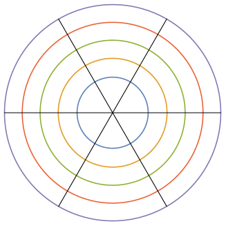
Figure 4. The nodal line of the disk eigenfunction $f_{3,5}(x)=J_{3}(j_{3,5}r)\cos(3\theta)$, which consists of $3$ diameters and $4$ circles.

References

- [1] J.-M. Azaïs, M. Wschebor, Level sets and extrema of random processes and fields, John Wiley & Sons Inc., Hoboken, NJ, 2009.
- [2] J. Bourgain, On Pleijel’s nodal domain theorem. Int. Math. Res. Not. IMRN 2015, no. 6, 1601–1612.
- [3] M.-C. Chang, H. Nguyen, O. Nguyen and V. Vu. Random eigenfunctions on flat tori: universality for the number of intersections. arXiv:1707.05255 [math.PR]
- [4] H. Donnelly, and C. Fefferman Nodal sets of eigenfunctions on Riemannian manifolds, Invent. Math. 93 (1988), 161–183.
- [5] P. Kurlberg and I. Wigman, Variation of the Nazarov-Sodin constant, available online https://arxiv.org/abs/1707.00766. Announcement C. R. Math. Acad. Sci. Paris 353 (2015), no. 2, 101–104.
- [6] M. Krishnapur, P. Kurlberg and I. Wigman. Nodal length fluctuations for arithmetic random waves, Ann. Math. (2) 177, no. 2, 699–737 (2013).
- [7] A. Logunov Nodal sets of Laplace eigenfunctions: polynomial upper estimates of the Hausdorff measure. Annals of Math., 187 (2018), Issue 1 221–239. arXiv:1605.02587 [math.AP]
- [8] A. Logunov Nodal sets of Laplace eigenfunctions: proof of Nadirashvili’s conjecture and of the lower bound in Yau’s conjecture. Annals of Math., 187 (2018), Issue 1 241–262. arXiv:1605.02589 [math.AP]
- [9] A. Logunov and E. Malinnikova Nodal sets of Laplace eigenfunctions: estimates of the Hausdorff measure in dimension two and three, arXiv:1605.02595 [math.AP]
- [10] D. Marinucci, G. Peccati, M. Rossi and I. Wigman, Non-universality of nodal length distribution for arithmetic random waves. Geom. Funct. Anal. 26 (2016), no. 3, 926–960.
- [11] R.C. McCann. Lower bounds for the zeros of Bessel functions. Proc. Amer. Math. Soc. 64 (1977), no. 1, 101–103.
- [12] G. Peccati and M. Rossi. Quantitative limit theorems for local functionals of arithmetic random waves. arXiv:1702.03765 [math.PR]
- [13] F. Nazarov and M. Sodin, On the number of nodal domains of random spherical harmonics. Amer. J. Math. 131 (2009), no. 5, 1337–1357.
- [14] Nazarov, F.; Sodin, M. Asymptotic laws for the spatial distribution and the number of connected components of zero sets of Gaussian random functions. Zh. Mat. Fiz. Anal. Geom. 12 (2016), no. 3, 205–278.
- [15] F. Oravecz, Z. Rudnick and I. Wigman The Leray measure of nodal sets for random eigenfunctions on the torus. Annales de l’institut Fourier, Volume 58 (2008) no. 1 , p. 299–335
- [16] Y. Rozenshein, The Number of Nodal Components of Arithmetic Random Waves. Int. Math. Res. Not. IMRN 2017, no. 22, 6990–7027. arXiv:1604.00638 [math.CA]
- [17] Z. Rudnick and I. Wigman. On the volume of nodal sets for eigenfunctions of the Laplacian on the torus. Ann. Henri Poincaré 9 (2008), no. 1, 109–130.
- [18] P. Swerling. Statistical properties of the contours of random surfaces. IRE Trans. IT-8 1962 315–321.