Optimal Control of Autonomous Vehicles Approaching A Traffic Light

Abstract

This paper devotes to the development of an optimal acceleration/speed profile for autonomous vehicles approaching a traffic light. The design objective is to achieve both short travel time and low energy consumption as well as avoid idling at a red light. This is achieved by taking full advantage of the traffic light information based on vehicle-to-infrastructure communication. The problem is modeled as a mixed integer programming, which is equivalently transformed into optimal control problems by relaxing the integer constraint. Then the direct adjoining approach is used to solve both free and fixed terminal time optimal control problems subject to state constraints. By an elaborate analysis, we are able to produce a real-time online analytical solution, distinguishing our method from most existing approaches based on numerical calculations. Extensive simulations are executed to compare the performance of autonomous vehicles under the proposed speed profile and human driving vehicles. The results show quantitatively the advantages of the proposed algorithm in terms of energy consumption and travel time.

I Introduction

The alarming state of existing transportation systems has been well documented. For instance, in 2014, congestion caused vehicles in urban areas to spend 6.9 billion additional hours on the road at a cost of an extra 3.1 billion gallons of fuel, resulting in a total cost estimated at $160 billion [1]. From a control and optimization standpoint, the challenges stem from requirements for increased safety, increased efficiency in energy consumption, and lower congestion both in highway and urban traffic. Connected and automated vehicles (CAVs), commonly known as self-driving or autonomous vehicles, provide an intriguing opportunity for enabling users to better monitor transportation network conditions and to improve traffic flow. Their proliferation has rapidly grown, largely as a result of Vehicle-to-X (or V2X) technology [2] which refers to an intelligent transportation system where all vehicles and infrastructure components are interconnected with each other. Such connectivity provides precise knowledge of the traffic situation across the entire road network, which in turn helps optimize traffic flows, enhance safety, reduce congestion, and minimize emissions. Controlling a vehicle to improve energy consumption has been studied extensively, e.g., see [3, 4, 5, 6]. By utilizing road topography information, an energy-optimal control algorithm for heavy diesel trucks is developed in [5]. Based on Vehicle-to-Vehicle (V2V) communication, a minimum energy control strategy is investigated in car-following scenarios in [6]. Another important line of research focuses on coordinating vehicles at intersections to increase traffic flow while also reducing energy consumption. Depending on the control objectives, work in this area can be classified as dynamically controlling traffic lights [7] and  as coordinating vehicles [8],[9],[10],[11]. More recently, an optimal control framework is proposed in [12] for CAVs to cross one or two adjacent intersections in an urban area. The state of art and current trends in the coordination of CAVs is provided in [13].

Our focus in this paper is on an optimal control approach for a single autonomous vehicle approaching an intersection in terms of energy consumption and taking advantage of traffic light information. The term “ECO-AND” short for “Economical Arrival and Departure”) is often used to refer to this problem. Its solution is made possible by vehicle-to-infrastructure (V2I) communication, which enables a vehicle to automatically receive signals from upcoming traffic lights before they appear in its visual range. For example, such a V2I communication system has been launched in Audi cars in Las Vegas by offering a traffic light timer on their dashboards: as the car approaches an intersection, a red traffic light symbol and a “time-to-go” countdown appear in the digital display and reads how long it will be before the traffic light ahead turns green [14]. Clearly, an autonomous vehicle can take advantage of such information in order to go beyond current “stop-and-go” to achieve “stop-free” driving. Along these lines, the problem of avoiding red traffic lights is investigated in [15, 16, 17, 18, 19]. The purpose in [15] is to track a target speed profile, which is generated based on the feasibility of avoiding a sequence of red lights. The approach uses model predictive control based on a receding horizon. The authors in [16] studied an energy-efficient driving strategy on roads with varying traffic lights and signals at intersections. with the goal of avoiding a red light instead of following the host vehicle driven by a human. Avoiding red lights with probabilistic information at multiple intersections was considered in [17], where the time horizon is discretized and deterministic dynamic programming is utilized to numerically compute the optimal control input. The work in [18] devises the optimal speed profile given the feasible target time, which is within some green light interval. A velocity pruning algorithm is proposed in [19] to identify feasible green windows, and a velocity profile is calculated numerically in terms of energy consumption.

Here, we investigate the optimal control problem of autonomous vehicles approaching a traffic light where the objective function is a weighted sum of both travel time and energy consumption. The problem is challenging due to the following reasons. First, finding a feasible green light interval leads to a Mixed Integer Programming (MIP) problem formulation. In general, solving MIP problems requires a significant amount of computation, and the optimality of the solution is not guaranteed due to the non-convexity of the problem involved with integer variables. The second reason comes from state constraints related to speed limits. The inclusion of bounds on state variables poses a significant challenge for most optimization methods. To overcome the above difficulties, we devise a two-step method. Specifically, we first address the problem without the traffic light constraint, which means that the terminal time is free, and the mixed integer constraints are removed. If the terminal time obtained from the free terminal time optimal control problem is within some green light interval, then the problem is solved. However, if the terminal time falls within some red light interval, then the optimal terminal time could be either the end of the previous green light interval or the beginning of the next green light interval by using the monotonicity property of the objective function. Then, we transform the original problem into a fixed terminal time optimal control problem. We solve the fixed terminal time optimal control problem with two different terminal times, and comparing the corresponding performances leads to the optimal solution of the original problem. All related optimal control problems with state constraints are solved by using the direct adjoining approach [20]. The main contributions of our paper are:

• Instead of solving this problem numerically as in [15] and [17], an analytical solution is obtained.

• For the free terminal time optimal control problem, it is easy to characterize the type of the optimal acceleration profile.

• Due to the on-line and real-time nature of the algorithm, the optimal control profile can be re-calculated as needed, for example when the optimal trajectory is interrupted by other road users due to safety constraints.

The remainder of this paper is organized as follows. The problem is formulated in Section II. In Section III, we present the methodology to solve the formulated problem, where the solution to the free terminal time optimal control problem is described in Subsection III-A, and the solution to the fixed terminal time optimal control problem is presented in Subsection III-B. Simulation results illustrating the use of the proposed algorithm are presented in Section IV. Section V summarizes our findings, concludes the paper and provides directions for future work.

II Problem Formulation

The dynamics of the vehicle are modeled by a double integrator

$$\dot{x}\left(t\right) =v\left(t\right),$$ (1)

$$\dot{v}\left(t\right) =u\left(t\right),$$ (2)

where $x\left(t\right),$ $v\left(t\right)$, and $u\left(t\right)$ are the position, velocity, and acceleration of the vehicle, respectively. At time $t_{0},$ the initial position and velocity are given as $x\left(t_{0}\right)=0$ and $v\left(t_{0}\right)=v_{0}$ respectively. Let us use $l$ to denote the distance to the traffic light, and $t_{p}$ the intersection crossing time of the vehicle. The traffic light switches between green and red at an intersection are dictated by a rectangular pulse signal $f\left(t\right)$ with a period $T$:

$$f\left(t\right)=\left\{\begin{array}[c]{ll}1&\text{for }kT\leq t\leq kT+DT,\\ 0&\text{for }kT+DT<t<\left(k+1\right)T,\end{array}\right.$$

where $f\left(t\right)=1$ indicates that the traffic light is green, and $f\left(t\right)=0$ indicates that the traffic light is red as shown in Fig. 1. The parameter $0<D<1$ is the fraction of the time period $T$ during which the traffic light is green, and $k\in\mathbb{Z}_{\geq 0}$ is a non-negative integer.

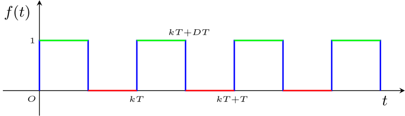
Figure 1: Traffic light signal

Our objective is to make the vehicle cross an intersection without stopping with the aid of traffic light information (TLI) as well as to minimize both travel time and energy consumption. Thus, we formulate the following problem:

Problem 1

ECO-AND Problem

$$\min_{u\left(t\right)}\quad\rho_{t}\left(t_{p}-t_{0}\right)+\rho_{u}\int_{t_{0}}^{t_{p}}u^{2}\left(t\right)dt$$ (3)

subject to

$$(\ref{dc1})\text{ and }(\ref{dc2}),$$ (4)

$$x\left(t_{p}\right)=l,$$ (5)

$$v_{\min}\leq v\left(t\right)\leq v_{\max}$$ (6)

$$u_{\min}\leq u\left(t\right)\leq u_{\max}$$ (7)

and

$$kT\leq t_{p}\leq kT+DT,$$ (8)

for some $k\in\mathbb{Z}_{\geq 0}$. In (3), the term $J^{t}=t_{p}-t_{0}$ is the travel time while $J^{u}=\int_{t_{0}}^{t_{p}}u^{2}\left(t\right)dt$ captures the energy consumption; see [21].

In order to normalize these two terms for the purpose of a well-defined optimization problem, first note that the maximum possible value of $J^{t}$ is $l/v_{\min}$. Depending on the relationship between $v_{\min}$, $v_{\max}$, $u_{\max}$ and $l$, there are two different cases for the maximum possible value of $J^{u}$. The first case is when the road length is long enough so that the vehicle can accelerate from $v_{\min}$ to $v_{\max}$ by using the maximum acceleration $u_{\max}$, i.e., when $l\geq v_{\min}\frac{v_{\max}-v_{\min}}{u_{\max}}+\frac{1}{2}\frac{\left(v_{\max}-v_{\min}\right)^{2}}{u_{\max}}$. In this case,

$$J^{u}=\int_{t_{0}}^{t_{p}}u_{\max}^{2}dt=\frac{v_{\max}-v_{\min}}{u_{\max}}u_{\max}^{2}=\left(v_{\max}-v_{\min}\right)u_{\max}\text{.}$$

The second case is when the road length is not long enough for the vehicle to accelerate to the maximum speed. According to the dynamics (1) and (2), we have

$$v_{\min}(t_{p}-t_{0})+\frac{1}{2}u_{\max}(t_{p}-t_{0})^{2}=l.$$

By solving the above quadratic equation, we are able to get

$$t_{p}-t_{0}=\frac{\sqrt{v_{\min}^{2}+2u_{\max}l}-v_{\min}}{u_{\max}}.$$

Therefore, in this case:

$$J^{u}=\int_{t_{0}}^{t_{p}}u_{\max}^{2}dt=\left(\sqrt{v_{\min}^{2}+2u_{\max}l}-v_{\min}\right)u_{\max}.$$

We can now specify the two weighting parameters $\rho_{t}$ and $\rho_{u}$ as follows: $\rho_{t}=\rho\frac{v_{\min}}{l}$ and

$$\rho_{u}=\left\{\begin{array}[c]{ll}\frac{1-\rho}{\left(v_{\max}-v_{\min}\right)u_{\max}}&\begin{array}[c]{l}\text{if }l\geq v_{\min}\frac{v_{\max}-v_{\min}}{u_{\max}}\\ \qquad+\frac{1}{2}\frac{\left(v_{\max}-v_{\min}\right)^{2}}{u_{\max}}\end{array}\\ \frac{1-\rho}{\left(\sqrt{v_{\min}^{2}+2u_{\max}l}-v_{\min}\right)u_{\max}}&\text{otherwise}\end{array}\right.$$

capturing the normalized trade-off between the travel time and energy consumption by setting $0\leq\rho\leq 1$. When $\rho=0$, the problem reduces to minimizing the energy consumption only; when $\rho=1$, we seek to minimize the travel time only.

In (6)-(7), the parameters $v_{\min}\geq 0$ and $v_{\max}>0$ are the minimum and maximum allowable speeds for road vehicles, respectively, while the parameters $u_{\min}$ and $u_{\max}$ are the maximum allowable deceleration and acceleration, respectively. Note that hen $u<0$, the vehicle decelerates due to braking and when $u>0$ the vehicle accelerates. Finally, the integer constraint (8) reflects the requirement that $t_{p}$ belongs to an interval when the light is green (see Fig. 1).

III Main Results

Problem 1 is a Mixed Integer Programming (MIP) problem. Existing approaches to such problems turn out to be computationally very demanding for off-line computation, not to mention obtaining analytical solutions in a real-time on-line context. We propose a two-step approach, which allows us to efficiently obtain an analytical solution on-line. The first step is to solve Problem 1 without the integer constraint (8). If the optimal arrival time $t_{p}^{\ast}$ is within some green light interval, then the problem is solved. However, if

$$kT+DT<t_{p}^{\ast}<kT+T,$$

for some $k$, then we solve Problem 1 twice with the constraint (8) replaced by $t_{p}=kD+DT$ and $t_{p}=kT+T$, respectively. We compare the performance obtained with different terminal times, and the solution produced by the one with better performance naturally yields the optimal solution.

Let us first introduce a lemma, which will be used frequently throughout the following analysis.

Lemma 1

Consider the vehicle’s dynamics (1) and (2) with the initial conditions $x_{0}$ and $v_{0}$. If the control input $u\left(t\right)=u$ is constant during the time interval $\left[t_{0},t_{1}\right]$, then

$$v\left(t_{1}\right) =v_{0}+u\left(t_{1}-t_{0}\right),$$

$$x\left(t_{1}\right) =x_{0}+v_{0}\left(t_{1}-t_{0}\right)+\frac{1}{2}u\left(t_{1}-t_{0}\right)^{2},$$

$$J^{u} =u^{2}\left(t_{1}-t_{0}\right);$$

If the control input $u\left(t\right)=u\left(t_{1}-t\right)$ with a constant $u$, then

$$v\left(t_{1}\right) =v_{0}+\frac{1}{2}u\left(t_{1}-t_{0}\right)^{2},$$

$$x\left(t_{1}\right) =x_{0}+v_{0}\left(t_{1}-t_{0}\right)+\frac{1}{3}u\left(t_{1}-t_{0}\right)^{3}\text{,}$$

$$J^{u} =\frac{1}{3}u^{2}\left(t_{1}-t_{0}\right)^{3}.$$

The proof is given in Appendix A.

In the following, we first seek the optimal solution to Problem 1 without the constraint (8), which is termed “free terminal time optimal control problem”.

III-A Free Terminal Time Optimal Control Problem

The free terminal time optimal control problem is given below.

Problem 2

Free Terminal Time Optimal Control Problem

$$\min_{u\left(t\right)}\rho_{t}\left(t_{p}-t_{0}\right)+\rho_{u}\int_{t_{0}}^{t_{p}}u^{2}\left(t\right)dt$$ (9)

subject to

$$(\ref{dc1})\text{ and }(\ref{dc2}),$$ (10)

$$x\left(t_{p}\right)=l,$$ (11)

$$v_{\min}\leq v\left(t\right)\leq v_{\max},$$ (12)

$$u_{\min}\leq u\left(t\right)\leq u_{\max},$$ (13)

where $\rho_{t}$ and $\rho_{u}$ are given in Section II.

From the objective function (9), it can be seen that a minimum energy consumption solution should avoid braking, that is, $u\left(t\right)\geq 0$ for $t\in\left[t_{0},t_{p}\right]$. We will show this fact in the following lemma.

Lemma 2

The optimal solution $u^{*}(t)$ to Problem 2 satisfies $u^{\ast}\left(t\right)\geq 0$ for all $t\in\left[t_{0},t_{p}^{*}\right]$.

The proof is given in Appendix B.

In addition, it follows from this lemma that whenever $v\left(\tau\right)=v_{\max}$ (which may not be possible in some cases), we must have $u\left(t\right)=0$ for all $t\in\left[\tau,t_{p}\right]$. Based on these observations, we can derive necessary conditions for the solution to Problem 2, which are summarized in the following theorem.

Theorem 1

Let $x^{\ast}\left(t\right)$, $v^{\ast}\left(t\right)$, $u^{\ast}\left(t\right)$, $t_{p}^{\ast}$ be an optimal solution to Problem 2 and assume that $\rho_{t}\neq 0$ and $\rho_{u}\neq 0$. Then, the optimal control $u^{\ast}\left(t\right)$ satisfies

$$u^{\ast}\left(t\right)=\arg\min_{0\leq u\left(t\right)\leq u_{\max}}\rho_{u}u^{2}+\frac{\rho_{t}}{v^{\ast}\left(t_{p}^{\ast}\right)}\left(t-\tau\right)u,$$ (14)

where $\tau$ is the first time on the optimal path when $v\left(\tau\right)=v_{\max}$ if $\tau<t_{p}$; $\tau=t_{p}^{\ast}$ otherwise.

Proof:

Here we use the direct adjoining approach in [20] to obtain necessary conditions for the optimal solution $u^{\ast}\left(t\right)$ and $t_{p}^{\ast}$. The Hamiltonian $H\left(v,u,\lambda\right)$ and Lagrangian $L\left(v,u,\lambda,\mu,\eta\right)$ are defined as

$$H\left(v,u,\lambda\right)=\rho_{u}u^{2}+\rho_{t}+\lambda_{1}v+\lambda_{2}u$$ (15)

and

$$L\left(v,u,\lambda,\mu,\eta\right)= H\left(v,u,\lambda\right)+\mu\left(u-u_{\max}\right)$$

$$+\eta_{1}\left(v_{\min}-v\right)+\eta_{2}\left(v-v_{\max}\right),$$ (16)

respectively, where $\lambda(t)=[\lambda_{1}(t)\text{ }\lambda_{2}(t)]^{T}$ and $\eta(t)=[\eta_{1}(t)\text{ }\eta_{2}(t)]^{T}$,

$$\mu\left(t\right)\geq 0\text{, }\mu\left(t\right)\left[u^{\ast}\left(t\right)-u_{\max}\right]=0,$$ (17)

$$\eta_{1}\left(t\right)\geq 0,\text{ }\eta_{2}\left(t\right)\geq 0,$$

$$\eta_{1}\left(t\right)\left[v_{\min}-v^{\ast}\left(t\right)\right]+\eta_{2}\left(t\right)\left[v^{\ast}\left(t\right)-v_{\max}\right]=0.$$ (18)

Note that we did not include the constraint $u\left(t\right)\geq u_{\min}$ since we have already established that the optimal control $u^{\ast}\left(t\right)\geq 0$ in the free terminal time optimal control problem in Lemma 2. Let us temporarily assume that both $\rho_{t}\neq 0$ and $\rho_{u}\neq 0$. According to Pontryagin’s minimum principle, the optimal control $u^{\ast}\left(t\right)$ must satisfy

$$u^{\ast}\left(t\right)=\arg\min_{0\leq u\left(t\right)\leq u_{\max}}H\left(v^{\ast}\left(t\right),u(t),\lambda\left(t\right)\right)\text{,}$$ (19)

which allows us to express $u^{\ast}\left(t\right)$ in terms of the costate $\lambda\left(t\right)$, resulting in

$$u^{\ast}\left(t\right)=\min\left\{u_{\max},-\frac{\lambda_{2}\left(t\right)}{2\rho_{u}}\right\},$$ (20)

with $\lambda_{2}\left(t\right)\leq 0$ due to Lemma 2. The Lagrange multiplier $\mu\left(t\right)$ is such that

$$\left.\frac{\partial L^{\ast}}{\partial u}\right|_{u=u^{\ast}\left(t\right)}=2\rho_{u}u^{\ast}\left(t\right)+\lambda_{2}\left(t\right)+\mu\left(t\right)=0.$$ (21)

Since we can always find $\mu\left(t\right)\geq 0$ to make (17) and (21) hold under the minimum principle (20), (17) and (21) can be considered as redundant conditions. For the costate $\lambda_{1}\left(t\right)$, we have

$$\dot{\lambda}_{1}\left(t\right)=-\frac{\partial L^{\ast}\left(t\right)}{\partial x}=0,$$

which means $\lambda_{1}(t)=\lambda_{1}$ is a constant. The costate $\lambda_{2}\left(t\right)$ satisfies

$$\dot{\lambda}_{2}\left(t\right)=-\frac{\partial L^{\ast}\left(t\right)}{\partial v}=-\lambda_{1}+\eta_{1}\left(t\right)-\eta_{2}\left(t\right)\text{.}$$ (22)

First, let us use a proof by contradiction to show that if $v^{*}\left(t\right)=v_{\min}$, then $t=t_{0}$. Assume that $v^{*}\left(t\right)=v_{\min}$ for $t\neq t_{0}$. Then, we must have $v^{*}\left(t\right)=v_{\min}$ for all $t\in\left[t_{0},t_{p}^{\ast}\right]$. This is because acceleration always precedes cruising at constant speed in the optimal control profile. If not, the vehicle would travel a longer time for the same trip using the same amount of energy. According to the system dynamics in (2), $u\left(t\right)=0$ for all $t\in\left[t_{0},t_{p}^{\ast}\right]$. Based on the minimum principle (20), $\lambda_{2}\left(t\right)=0$ for all $t\in\left[t_{0},t_{p}^{\ast}\right]$. From (18), we know that $\eta_{2}\left(t\right)=0$ for all $t\in\left[t_{0},t_{p}^{\ast}\right]$. Since the terminal time $t_{p}$ is unspecified, there is a necessary transversality condition for $t_{p}^{\ast}$ to be optimal, namely, $H\left(v^{*}(t_{p}^{\ast}),u^{*}(t_{p}^{*}),\lambda(t_{p}^{\ast})\right)=0,$ that is,

$$\rho_{u}u^{*}\left(t_{p}^{\ast}\right)^{2}+\rho_{t}+\lambda_{1}v^{\ast}\left(t_{p}^{\ast}\right)+\lambda_{2}\left(t_{p}^{\ast}\right)u\left(t_{p}^{\ast}\right)=0\text{.}$$ (23)

Since $u^{*}\left(t_{p}^{\ast}\right)=0,$ we must have $\lambda_{1}<0$ according to (23). Then, we obtain $\dot{\lambda}_{2}\left(t\right)>0$ from (22), which contradicts $\lambda_{2}\left(t\right)=0$ for $t\in\left[t_{0},t_{p}^{\ast}\right]$. We have thus established that if $v^{*}\left(t\right)=v_{\min}$, then $t=t_{0}$. Next, we will show that $\lambda_{2}\left(t\right)$ has no discontinuities. Since it is impossible that $v\left(t\right)=v_{\min}$ for $t\neq t_{0}$, the costate trajectory $\lambda_{2}\left(t\right)$ may jump only at some time $\tau$ when $v\left(\tau\right)=v_{\max}$. The condition

$$H^{\ast}\left(\tau^{-}\right)=H^{\ast}\left(\tau^{+}\right),$$

can be written as

$$\rho_{u}u^{\ast}\left(\tau^{-}\right)^{2}+\lambda_{2}\left(\tau^{-}\right)u^{\ast}\left(\tau^{-}\right)$$

$$\qquad=\rho_{u}u^{\ast}\left(\tau^{+}\right)^{2}+\lambda_{2}\left(\tau^{+}\right)u^{\ast}\left(\tau^{+}\right),$$ (24)

where $\tau^{+}$ and $\tau^{-}$ denote the left-hand side and the right-hand side limits, respectively. We know from Lemma 2 that $u^{\ast}\left(t\right)=0,$ for $t\in\left[\tau,t_{p}^{\ast}\right]$. Therefore, from (24), we obtain

$$\rho_{u}u^{\ast}\left(\tau^{-}\right)^{2}+\lambda_{2}\left(\tau^{-}\right)u^{\ast}\left(\tau^{-}\right)=0\text{.}$$ (25)

According to (20), we either have $u^{\ast}\left(\tau^{-}\right)=-\frac{\lambda_{2}\left(\tau^{-}\right)}{2\rho_{u}}$ or $u^{\ast}\left(\tau^{-}\right)=u_{\max}$. When $u^{\ast}\left(\tau^{-}\right)=-\frac{\lambda_{2}\left(\tau^{-}\right)}{2\rho_{u}},$ (25) becomes

$$-\rho_{u}u^{\ast}\left(\tau^{-}\right)^{2}=0,$$

which implies $u^{\ast}\left(\tau^{-}\right)=\lambda_{2}\left(\tau^{-}\right)=0$. When $u^{\ast}\left(\tau^{-}\right)=u_{\max},$ (25) becomes

$$u_{\max}=\frac{-\lambda_{2}\left(\tau^{-}\right)}{\rho_{u}},$$

which contradicts the condition (20) where $u_{\max}=\frac{-\lambda_{2}\left(\tau^{-}\right)}{2\rho_{u}}$. Therefore, only the case $u^{\ast}\left(\tau^{-}\right)=\lambda_{2}\left(\tau^{-}\right)=0$ is possible. In other words, the costate trajectory $\lambda_{2}\left(t\right)$ has no discontinuities, and the following jump conditions:

$$\lambda_{2}\left(\tau^{-}\right)=\lambda_{2}\left(\tau^{+}\right)-\zeta_{1}\left(\tau\right)+\zeta_{2}\left(\tau\right),$$ (26)

and

$$\zeta_{1}\left(\tau\right)\geq 0,\zeta_{2}\left(\tau\right)\geq 0,$$

$$\zeta_{1}\left(\tau\right)\left[v_{\min}-v^{\ast}\left(\tau\right)\right]+\zeta_{2}\left(\tau\right)\left[v^{\ast}\left(\tau\right)-v_{\max}\right]=0,$$ (27)

are always satisfied with $\zeta_{1}\left(\tau\right)=\zeta_{2}\left(\tau\right)=0$. Next, we will show that $\lambda_{2}\left(t_{p}^{\ast}\right)=0$. At the terminal time $t_{p}^{*}$, the following transversality conditions hold:

$$\lambda_{2}\left(t_{p}^{\ast-}\right) = \gamma_{1}\left.\frac{\partial}{\partial v}\left[v_{\min}-v\right]\right|_{v=v^{\ast}\left(t_{p}^{\ast}\right)}$$

$$+\gamma_{2}\left.\frac{\partial}{\partial v}\left[v-v_{\max}\right]\right|_{v=v^{\ast}\left(t_{p}^{\ast}\right)}$$

that is,

$$\lambda_{2}\left(t_{p}^{*-}\right)=-\gamma_{1}+\gamma_{2},$$ (28)

where

$$\gamma_{1}\geq 0,\text{ }\gamma_{2}\geq 0,$$

$$\gamma_{1}\left[v_{\min}-v^{\ast}\left(t_{p}^{*}\right)\right]+\gamma_{2}\left[v^{\ast}\left(t_{p}^{*}\right)-v_{\max}\right]=0.$$ (29)

If $v_{\min}<v^{*}\left(t_{p}^{\ast}\right)<v_{\max}$, then $\gamma_{1}=\gamma_{2}=0$, which leads to $\lambda_{2}\left(t_{p}^{\ast}\right)=0$ by the continuity of $\lambda_{2}\left(t\right)$. When $v^{*}\left(t_{p}^{\ast}\right)=v_{\max},$ then $u^{*}\left(t_{p}^{\ast}\right)=0$, which results in $\lambda_{2}\left(t_{p}^{\ast}\right)=0$ according to (20). Last, we will show that $\eta_{1}\left(t\right)=0$, and

$$\eta_{2}\left(t\right)=\left\{\begin{array}[]{cc}0&\text{for }t\in\left[t_{0},\tau\right)\\ -\lambda_{1}&\text{for }t\in\left[\tau,t_{p}^{\ast}\right]\end{array}\right.$$

Since $H\left(v,u,\lambda\right)$ is not an explicit function of time $t$, it follows that

$$\frac{dH^{\ast}\left(t\right)}{dt}=0,$$

that is,

$$\left[2\rho_{u}u^{\ast}\left(t\right)+\lambda_{2}\left(t\right)\right]\dot{u}^{\ast}\left(t\right)+\left[\eta_{1}\left(t\right)-\eta_{2}\left(t\right)\right]u^{\ast}\left(t\right)=0.$$ (30)

The first term $\left[2\rho_{u}u^{\ast}\left(t\right)+\lambda_{2}\left(t\right)\right]\dot{u}^{\ast}\left(t\right)$ is always zero since when $u^{\ast}\left(t\right)\neq u_{\max}$, $2\rho_{u}u^{\ast}\left(t\right)+\lambda_{2}^{\ast}\left(t\right)=0$ according to (20), and when $u^{\ast}\left(t\right)=u_{\max}$, $\dot{u}^{\ast}\left(t\right)=0$. The condition (30) can thus be reduced to

$$\left[\eta_{1}\left(t\right)-\eta_{2}\left(t\right)\right]u^{\ast}\left(t\right)=0.$$ (31)

When $v_{0}=v_{\min}$, we have $\eta_{2}\left(t_{0}\right)=0$ from the fact that if $v^{*}\left(t\right)=v_{\min}$, then $t=t_{0}$ shown earlier and from (18). Condition (31) then implies

$$\eta_{1}\left(t_{0}\right)u^{\ast}\left(t_{0}\right)=0\text{.}$$

Since $u^{\ast}\left(t_{0}\right)>0$, we can get $\eta_{1}\left(t_{0}\right)=0$. For $t\neq t_{0},$ $\eta_{1}\left(t\right)=0$ since $v(t)>v_{\min}$ for $t\neq t_{0}$. Therefore, for any $v_{0},$ we have $\eta_{1}\left(t\right)=0$. It is easy to get from (18) that $\eta_{2}\left(t\right)=0$ for $t\in\left[t_{0},\tau\right)$. For $t\in\left[\tau,t_{p}^{\ast}\right]$, $\eta_{2}\left(t\right)=-\lambda_{1}$ satisfies the condition (18) and $\dot{\lambda}_{2}\left(t\right)=0$ in (22). Based on the above observations, the differential equation (22) becomes

$$\dot{\lambda}_{2}\left(t\right)=-\lambda_{1}$$ (32)

for $t\in\left[t_{0},\tau\right)$. From (23), we have $-\lambda_{1}=\frac{\rho_{t}}{v^{\ast}\left(t_{p}^{\ast}\right)}$ since $u^{\ast}\left(t_{p}^{\ast}\right)=0$. Solving the differential equation (32), we have

$$\lambda_{2}\left(t\right)=\frac{\rho_{t}}{v^{\ast}\left(t_{p}^{\ast}\right)}\left(t-\tau\right)$$ (33)

for $t\in\left[t_{0}\,\tau\right].$ In the case that $v^{\ast}\left(t_{p}^{\ast}\right)<v_{\max}$, we simply let $\tau=t_{p}^{\ast}$ in (33). The proof is completed by substituting (33) for $\lambda_{2}\left(t\right)$ in (19). ∎

Recall that the theorem was proved under the assumption that $\rho_{t}\neq 0$ and $\rho_{u}\neq 0$. The special cases when either $\rho_{t}=0$ or $\rho_{u}=0$ are considered in the following two corollaries.

Corollary 2

Let $x^{\ast}\left(t\right)$, $v^{\ast}\left(t\right)$, $u^{\ast}\left(t\right)$, $t_{p}^{\ast}$ be an optimal solution to Problem 2 when $\rho_{t}=0$. Then, the optimal control $u^{\ast}\left(t\right)$ satisfies

$$u^{\ast}\left(t\right)=0,$$ (34)

for all $t\in[t_{0},t_{p}^{\ast}]$.

Corollary 3

Let $x^{\ast}\left(t\right)$, $v^{\ast}\left(t\right)$, $u^{\ast}\left(t\right)$, $t_{p}^{\ast}$ be an optimal solution to Problem 2 when $\rho_{u}=0$. Then, the optimal control $u^{\ast}\left(t\right)$ satisfies

$$u^{\ast}\left(t\right)=\left\{\begin{array}[c]{ll}u_{\max}&\text{for }t\in\left[t_{0},\tau\right),\\ 0&\text{for }t\in\left[\tau,t_{p}^{\ast}\right],\end{array}\right.$$ (35)

where $\tau$ is the first time on the optimal path when $v^{\ast}(\tau)=v_{\max}$.

The proofs of the above two corollaries are straightforward by setting $\rho_{t}=0$ and $\rho_{u}=0$, respectively, in (14) in Theorem 1.

Based on the vehicle dynamics (1) and (2), the initial conditions $x\left(t_{0}\right)=0$ and $v\left(t_{0}\right)=v_{0},$ and the terminal condition $x^{\ast}\left(t_{p}^{\ast}\right)=l$, the optimal control law (14) and the optimal time $t_{p}^{\ast}$ can be uniquely determined. In the following, we will classify the results into different cases dependent on the values of the model parameters. In order to do so, we define two functions:

$$f\left(v_{0}\right) =l-\frac{v_{\max}^{2}-v_{0}^{2}}{2u_{\max}}-u_{\max}v_{\max}^{2}\frac{\rho_{u}}{\rho_{t}}+\frac{1}{6}u_{\max}^{3}v_{\max}^{2}\frac{\rho_{u}^{2}}{\rho_{t}^{2}},$$

$$g\left(v_{0}\right) =\,l-2v_{0}\sqrt{\left(v_{\max}-v_{0}\right)v_{\max}\frac{\rho_{u}}{\rho_{t}}}$$

$$-\frac{4}{3}\left(v_{\max}-v_{0}\right)\sqrt{\left(v_{\max}-v_{0}\right)v_{\max}\frac{\rho_{u}}{\rho_{t}}}.$$

Depending on the signs of these two functions, the optimal solution consisting of $u^{\ast}\left(t\right)$ and $t_{p}^{\ast}$ can be classified as shown in Table I with all detailed calculations provided in Appendix C. Referring to this table, the optimal control is parameterized by the following function

$$\Phi\left(t|a,b,c\right)=\left\{\begin{array}[c]{ll}u_{\max}&\text{when }t\leq a\\ c(t-b)&\text{when }a<t<b\\ 0&\text{when }t\geq b\end{array}\right.$$

TABLE I: Optimal solution classification for Problem 2

	$\frac{v_{0}}{v_{\max}}<1-u_{\max}^{2}\frac{\rho_{u}}{\rho_{t}}$		$1-u_{\max}^{2}\frac{\rho_{u}}{\rho_{t}}\leq\frac{v_{0}}{v_{\max}}$
	$f\left(v_{0}\right)\geq 0$	$f\left(v_{0}\right)<0$	$g\left(v_{0}\right)\geq 0$	$g\left(v_{0}\right)<0$
$u^{\ast}$	$\Phi\left(t|t_{1},t_{2},\frac{\rho_{t}}{2\rho_{u}v_{\max}}\right)$	$\Phi\left(t|t_{3},-,\frac{\rho_{t}}{2\rho_{u}v_{1}}\right)$	$\Phi\left(t|-,t_{4},\frac{\rho_{t}}{2\rho_{u}v_{\max}}\right)$	$\Phi\left(t|-,-,\frac{\rho_{t}}{2\rho_{u}v_{2}}\right)$
$t_{p}^{\ast}$	$\delta_{1}$	$\delta_{2}$	$\delta_{3}$	$\delta_{4}$

The parameters shown in Table I are defined as follows:

$$t_{1} =t_{0}+\frac{\left(1-u_{\max}^{2}\frac{\rho_{u}}{\rho_{t}}\right)v_{\max}-v_{0}}{u_{\max}},\text{ }t_{3}=t_{0}+\frac{v_{1}-v_{0}}{u_{\max}},$$

$$t_{2} =t_{1}+2u_{\max}v_{\max}\frac{\rho_{u}}{\rho_{t}},\text{ }t_{4}=t_{0}+2\sqrt{\left(v_{\max}-v_{0}\right)v_{\max}\frac{\rho_{u}}{\rho_{t}}},$$

where

$$v_{1}=\sqrt{\frac{2u_{\max}l+v_{0}^{2}}{1+\frac{4u_{\max}^{2}}{1-\frac{\rho_{u}}{\rho_{t}}u_{\max}^{2}}\frac{\rho_{u}}{\rho_{t}}+\frac{8}{3}\frac{u_{\max}^{4}}{\left(1-\frac{\rho_{u}}{\rho_{t}}u_{\max}^{2}\right)^{2}}\frac{\rho_{u}^{2}}{\rho_{t}^{2}}}}$$

and $v_{2}$ is the solution of the following equation:

$$l=\frac{2}{3}\left(v_{0}+2v_{2}\right)\sqrt{\left(v_{2}-v_{0}\right)v_{2}\frac{\rho_{u}}{\rho_{t}}}.$$

The parameters $\delta_{1},\delta_{2},\delta_{3},\delta_{4}$ specifying in Table I the optimal time $t_{p}^{\ast}$ when the vehicle arrives at the traffic light in each of the four possible cases are given below:

$$\delta_{1} =t_{2}+\frac{f\left(v_{0}\right)}{v_{\max}},$$

$$\delta_{2} =t_{3}+2u_{\max}\frac{v_{1}}{1-\frac{\rho_{u}}{\rho_{t}}u_{\max}^{2}}\frac{\rho_{u}}{\rho_{t}},$$

$$\delta_{3} =t_{4}+\frac{g(v_{0})}{v_{\max}},$$

$$\delta_{4} =t_{0}+2\sqrt{\left(v_{2}-v_{0}\right)v_{2}\frac{\rho_{u}}{\rho_{t}}}.$$

Remark 1

This remark pertains to the underlying criteria for the optimal solution classification in Table I. The first row determines whether or not the maximum acceleration $u_{\max}$ will be used for a given initial speed $v_{0}$. The optimality conditions tell us that the vehicle starts with the maximum acceleration when the initial speed is relatively slow. The second row determines if the road length $l$ is large enough for a vehicle to reach its maximum speed for a given initial speed $v_{0}$. In general, the optimal control contains three phases: full acceleration, linearly decreasing acceleration, and no acceleration. The first column specifies the case where all three phases are included with switches defined by $t_{1}$, $t_{2}$. The second column corresponds to the case of low initial speeds and short-length roads. Under optimal control in this case, the vehicle starts with full acceleration, but the road length is so short that the maximum speed cannot be reached. Therefore, the optimal control contains only the first two phases. The third column corresponds to the case of large initial speeds and long-length roads. The vehicle starts with linearly decreasing acceleration, and then proceeds with no acceleration when the speed reaches the limit $v_{\max}$. Here, the optimal control contains only the last two phases. The last column corresponds to the case of large initial speeds and short-length roads. Therefore, the vehicle uses only linearly decreasing acceleration.

III-B Fixed Terminal Time Optimal Control Problem

In this section, we consider the case where the optimal time $t_{p}^{\ast}$ obtained in the free terminal time optimal control problem 2 is within some red light interval, that is,

$$kT+DT<t_{p}^{\ast}<kT+T,$$

In this case, the candidate optimal arrival time $t_{p}^{\ast}$ in Problem 1 is either $kT+DT$ or $kT+T$. Therefore, we can compare the performance obtained under either one of these two terminal times, and select the one with better performance to determine the optimal arrival time for Problem 1. In both cases, the travel time is now fixed, hence the only objective is to minimize the energy consumption. Thus, we have the following problem formulation:

Problem 3

Fixed Terminal Time Optimal Control Problem

$$\min_{u\left(t\right)}\int_{t_{0}}^{t_{p}}u^{2}\left(t\right)dt$$ (36)

subject to

$$(\ref{dc1})\text{ and }(\ref{dc2})$$ (37)

$$x\left(t_{p}\right)=l$$ (38)

$$t_{p}=kT+DT\text{ or }kT+T$$ (39)

$$v_{\min}\leq v\left(t\right)\leq v_{\max}$$ (40)

$$u_{\min}\leq u\left(t\right)\leq u_{\max}$$ (41)

III-B1 Arrival Time $t_{p}=kT+DT$

In this case, it is clear that that the vehicle must use less time than the one specified by $t_{p}^{\ast}$ in Problem 2 and higher acceleration. Define a function

$$h\left(v_{0}\right)=\left\{\begin{array}[c]{ll}v_{0}t_{p}+\frac{1}{2}u_{\max}t_{p}^{2}-l&\text{for }t_{p}\leq\frac{v_{\max}-v_{0}}{u_{\max}}\\ v_{\max}t_{p}-\frac{1}{2}\frac{\left(v_{\max}-v_{0}\right)^{2}}{u_{\max}}-l&\text{for }t_{p}>\frac{v_{\max}-v_{0}}{u_{\max}}\end{array}\right.$$

Observe that the terminal time $t_{p}=kT+DT$ is possible if and only if $h\left(v_{0}\right)\geq 0$. The main result for this case is given in the following theorem.

Theorem 4

Let $x^{\ast}\left(t\right)$, $v^{\ast}\left(t\right)$, $u^{\ast}\left(t\right)$ be an optimal solution to Problem 3 with $t_{p}=kT+DT$. Then, the optimal control $u^{\ast}\left(t\right)$ satisfies

$$u^{\ast}\left(t\right)=\arg\min_{0\leq u\left(t\right)\leq u_{\max}}u^{2}+\frac{u^{\ast}\left(t_{0}\right)^{2}\left(t-\tau\right)u}{v_{0}-v^{\ast}\left(t_{p}\right)+\left(\tau-t_{0}\right)u^{\ast}\left(t_{0}\right)}\text{,}$$

where $\tau$ is the first time on the optimal path when $v\left(\tau\right)=v_{\max}$ if $\tau<t_{p}$; $\tau=t_{p}^{\ast}$ otherwise.

Proof:

Similar to the proof of Theorem 1, we will use the direct adjoining approach [20] to solve the fixed terminal time optimal control problem. The Hamiltonian $H\left(v,u,\lambda\right)$ and Lagrangian $L\left(v,u,\lambda,\mu,\eta\right)$ are defined as

$$H(u,v,\lambda)=u^{2}+\lambda_{1}v+\lambda_{2}u,$$

and

$$L(u,v,\lambda,\mu,\eta)= \,H+\mu\left(u-u_{\max}\right)$$

$$+\eta_{1}\left(v_{\min}-v\right)+\eta_{2}\left(v-v_{\max}\right),$$

respectively, where $\lambda(t)=[\lambda_{1}(t)\text{ }\lambda_{2}(t)]^{T}$ and $\eta(t)=[\eta_{1}(t)\text{ }\eta_{2}(t)]^{T}$, and

$$\mu\left(t\right)\geq 0,\mu\left(t\right)\left[u^{\ast}\left(t\right)-u_{\max}\right]=0,$$

$$\eta_{1}\left(t\right)\geq 0,\eta_{2}\left(t\right)\geq 0,$$

$$\eta_{1}\left(t\right)\left[v_{\min}-v^{\ast}\left(t\right)\right]+\eta_{2}\left(t\right)\left[v^{\ast}\left(t\right)-v_{\max}\right]=0.$$

Note that, as in the the proof of Theorem 1, $u^{\ast}\left(t\right)\geq 0$ for all $t$, therefore, the constraint $u\left(t\right)\geq u_{\min}$ is relaxed, and

$$u^{\ast}\left(t\right)=\arg\min_{0\leq u\left(t\right)\leq u_{\max}}u^{2}+\lambda_{2}u\text{.}$$ (42)

which implies that

$$u^{\ast}\left(t\right)=\min\left\{u_{\max},-\frac{\lambda_{2}\left(t\right)}{2}\right\}\text{,}$$

and $\lambda_{2}\left(t\right)\leq 0$. From the proof of Theorem 1, we know that $\mu\left(t\right)$ is a redundant variable, and $\lambda_{1}$ is a constant. Let us first assume that

$$l>v_{\min}t_{p}.$$

Note that the case of $l=v_{\min}t_{p}$ cannot occur when $t_{p}=kT+DT$ (however, it may occur when $t_{p}=kT+T$ and this case will be discussed later). Again, we can prove the fact that $v\left(t\right)=v_{\min}$ happens only at $t=t_{0}$ but without using the transversality condition as we did in the free terminal time optimal control problem. The property that $\lambda_{2}\left(t\right)$ has no discontinuities also still holds. The costate $\lambda_{2}(t)$ satisfies

$$\dot{\lambda}_{2}\left(t\right)=-\lambda_{1}+\eta_{1}\left(t\right)-\eta_{2}\left(t\right)\text{.}$$ (43)

Similarly, we can show that $\eta_{1}\left(t\right)=0$, and (43) reduces to

$$\dot{\lambda}_{2}\left(t\right)=-\lambda_{1}$$ (44)

for $t\in\left[t_{0},\tau\right)$ and $\lambda_{2}\left(\tau\right)=0$. By solving the differential equation (44), we get

$$\lambda_{2}\left(t\right)=-\lambda_{1}\left(t-\tau\right).$$ (45)

Again since the Hamiltonian is not an explicit function of time, by the condition

$$H\left(t_{0}\right)=H\left(t_{p}\right)\text{,}$$

we have

$$u^{\ast}\left(t_{0}\right)^{2}+\lambda_{1}v^{\ast}\left(t_{0}\right)-\lambda_{1}\left(t_{0}-\tau\right)u^{\ast}\left(t_{0}\right)=\lambda_{1}v^{\ast}\left(t_{p}\right)$$ (46)

where the fact that $\lambda_{2}(t_{p})=u^{*}(t_{p})=0$ has been used. From (46), we can obtain

$$\lambda_{1}=\frac{u^{\ast}\left(t_{0}\right)^{2}}{v^{\ast}\left(t_{p}\right)+\left(t_{0}-\tau\right)u^{\ast}\left(t_{p}\right)-v^{\ast}\left(t_{0}\right)}$$ (47)

For $t\in[\tau,t_{p}]$, we can just let $\eta_{2}(t)=-\lambda_{1}$. If $v^{*}(t_{p})<v_{\max}$, then $\tau=t_{p}$ in (46). The proof is completed by substituting $\lambda_{1}$ in (47) into (45), and then $\lambda_{2}$ into (42). ∎

Given the terminal time $kT+DT$ and the road length $l$, the value of $v_{0}$ can be classified into one of five cases as shown in Table II. Note that if Case $i$ is infeasible for some $v_{0}$ and the given parameters, we can treat $J_{i}^{u}$ as infinity.

TABLE II: Optimal solution classification for Problem 3 with $t_{p}=kT+DT$

	Optimal Control	Performance
Case I	$u_{0}^{*}=u_{\max}$ and $\dot{u}^{*}\left(t\right)=0$	$J_{1}^{u}$
Case II	$u^{\ast}\left(t_{0}\right)=u_{\max}$ and $v^{\ast}\left(t_{p}\right)=v_{\max}$	$J_{2}^{u}$
Case III	$u^{\ast}\left(t_{0}\right)=u_{\max}$ and $v^{\ast}\left(t_{p}\right)<v_{\max}$	$J_{3}^{u}$
Case IV	$u_{0}^{\ast}<u_{\max}$ and $v^{\ast}\left(t_{p}\right)=v_{\max}$	$J_{4}^{u}$
Case V	$u_{0}^{\ast}<u_{\max}$ and $v^{\ast}\left(t_{p}\right)<v_{\max}$	$J_{5}^{u}$

The performances associated with each case in Table II as well as the detailed calculations are given in Appendix D. After obtaining the performance for each cases with $t_{p}=kT+DT$, we select the one with the smallest energy consumption, that is,

$$J_{u}^{kT+DT}=\min\left\{J_{1}^{u},\ldots J_{5}^{u}\right\},$$

with the corresponding optimal acceleration profile.

III-B2 Arrival Time $t_{p}=kT+T$

In this case, the vehicle must use less acceleration than in the free terminal time case. Depending on the initial speed $v_{0}$, there are three cases to consider. First, if

$$l=v_{0}\left(kT+T-t_{0}\right),$$

then the vehicle can cruise through the intersection with the constant speed $v_{0}$ without any acceleration (Case VI in Table III). The energy consumption in this case is

$$J_{6}^{u}=0\text{.}$$

If, on the other hand,

$$l>v_{0}\left(kT+T-t_{0}\right),$$

then the problem can be solved using the result of the case $t_{p}=kT+DT$ analyzed above. Finally, if

$$l<v_{0}\left(kT+T-t_{0}\right)\text{,}$$

then the vehicle must decelerate to reach the traffic light while in its green state. Therefore, the control input is only subject to the constraint

$$u_{\min}\leq u\left(t\right)\leq 0\text{.}$$

The main result in this case is given in the following theorem.

Theorem 5

Let $x^{\ast}\left(t\right)$, $v^{\ast}\left(t\right)$, $u^{\ast}\left(t\right)$ be an optimal solution to Problem 3 with $t_{p}=KT+T$. Then, the optimal solution $u^{\ast}\left(t\right)$ satisfies

$$u^{\ast}\left(t\right)=\arg\min_{u_{\min}\leq u\left(t\right)\leq 0}u^{2}+\frac{u^{\ast}\left(t_{0}\right)^{2}\left(\tau-t\right)u}{v^{\ast}\left(t_{p}\right)-v_{0}-\left(\tau-t_{0}\right)u^{\ast}\left(t_{0}\right)},$$

where $\tau$ is the first time on the optimal path when $v\left(\tau\right)=v_{\max}$ if $\tau<t_{p}$; $\tau=t_{p}^{\ast}$ otherwise.

Proof:

The Hamiltonian $H\left(u,v,\lambda\right)$ and the Lagrangian $L\left(u,v,\lambda,\mu,\eta\right)$ are defined as

$$H\left(u,v,\lambda\right)=u^{2}+\lambda_{1}v+\lambda_{2}u$$

and

$$L\left(u,v,\lambda,\mu,\eta\right) =H\left(u,v,\lambda\right)+\mu\left(u_{\min}-u\right)$$

$$+\eta_{1}\left(v_{\min}-v\right)+\eta_{2}\left(v-v_{\max}\right)\text{,}$$

respectively, where $\lambda(t)=\left[\lambda_{1}(t),\lambda_{2}(t)\right]^{T}$, $\eta(t)=\left[\eta_{1}(t),\eta_{2}(t)\right]^{T}$, and

$$\mu\left(t\right)\geq 0,\text{ }\mu\left(t\right)\left[u_{\min}-u^{\ast}\left(t\right)\right]=0,$$

$$\eta_{1}\left(t\right)\geq 0,\text{ }\eta_{2}\left(t\right)\geq 0,$$

$$\eta_{1}\left(t\right)\left[v_{\min}-v^{\ast}\left(t\right)\right]+\eta_{2}\left(t\right)\left[v^{\ast}\left(t\right)-v_{\max}\right]=0.$$

As before, we do not include the constraint $u\left(t\right)\leq u_{\max}$ since we have already established in Lemma 2 that $u^{\ast}\left(t\right)\leq 0$.

According to Pontryagin’s minimum principle, the optimal control $u^{\ast}\left(t\right)$ must satisfy

$$u^{\ast}\left(t\right)=\arg\min_{u_{\min}\leq u\left(t\right)\leq 0}H\left(v^{\ast}\left(t\right),u^{\ast}\left(t\right),\lambda\left(t\right)\right)$$

which allows us to express $u^{\ast}\left(t\right)$ in terms of the costate $\lambda\left(t\right)$, that is,

$$u^{\ast}\left(t\right)=\max\left\{u_{\min},-\frac{\lambda_{2}\left(t\right)}{2}\right\}$$ (48)

with $\lambda_{2}\left(t\right)\geq 0$. The Lagrange multiplier $\mu\left(t\right)$ is redundant as before. The costate $\lambda_{1}$ is a constant. The co-state $\lambda_{2}\left(t\right)$ satisfies

$$\dot{\lambda}_{2}\left(t\right)=-\frac{\partial L^{\ast}}{\partial v}=-\lambda_{1}+\eta_{1}^{\ast}\left(t\right)-\eta_{2}^{\ast}\left(t\right)\text{.}$$

First, it is easy to see that $v_{0}\neq v_{\min}$. Let $\tau$ be the first time that $v\left(\tau\right)=v_{\min}$, then

$$u^{\ast}\left(t\right)=0$$

for $t\geq\tau$. Again, since the Hamiltonian is not an explicit function of time, by the condition

$$H^{\ast}\left(\tau^{-}\right)=H^{\ast}\left(\tau^{+}\right),$$

we have

$$u^{\ast}\left(\tau^{-}\right)^{2}+\lambda_{2}\left(\tau^{-}\right)u^{\ast}\left(\tau^{-}\right)=0\text{.}$$ (49)

According to (48), we either have $u^{\ast}\left(\tau^{-}\right)=u_{\min}$ or $u^{\ast}\left(\tau^{-}\right)=-\frac{\lambda_{2}\left(\tau^{-}\right)}{2}$. When $u^{\ast}\left(\tau^{-}\right)=u_{\min}$, the above equality becomes

$$u_{\min}^{2}+\lambda_{2}\left(\tau^{-}\right)u_{\min}=0\text{,}$$

which contradicts the minimum principle (48); when $u^{\ast}\left(\tau^{-}\right)=-\frac{\lambda_{2}\left(\tau^{-}\right)}{2}$, (49) becomes

$$u^{2}\left(\tau^{-}\right)-2u^{2}\left(\tau^{-}\right)=0.$$

Therefore, only $\lambda_{2}\left(\tau^{-}\right)=u^{\ast}\left(\tau^{-}\right)=0$ is possible, that is to say, $\lambda_{2}$ and $u^{\ast}$ have no discontinuities at $\tau$.

At the terminal time $t_{p}$, the following costate boundary condition holds:

$$\lambda_{2}\left(t_{p}^{\ast-}\right) =\gamma_{1}\left.\frac{\partial}{\partial v}\left[v_{\min}-v\right]\right|_{v=v^{\ast}\left(t_{p}^{\ast}\right)}$$

$$+\gamma_{2}\left.\frac{\partial}{\partial v}\left[v-v_{\max}\right]\right|_{v=v^{\ast}\left(t_{p}^{\ast}\right)}$$

that is,

$$\lambda_{2}\left(t_{p}^{-}\right)=-\gamma_{1}+\gamma_{2}$$

and

$$\gamma_{1}\geq 0,\text{ }\gamma_{2}\geq 0,\text{ }\gamma_{1}\left[v_{\min}-v^{\ast}\left(t_{p}\right)\right]+\gamma_{2}\left[v^{\ast}\left(t_{p}\right)-v_{\max}\right]=0\text{.}$$

At $t_{p}$, we know that $v^{\ast}\left(t_{p}\right)\neq v_{\max}$. Thus, $\gamma_{2}=0$. Likewise, it is easy to obtain $\gamma_{1}=0$. Therefore, we have

$$\lambda_{2}\left(t_{p}\right)=0\text{.}$$

Since the Hamiltonian is not an explicit function of time, the condition

$$\frac{dH^{\ast}\left(t\right)}{dt}=0,$$

implies that

$$\left[2u^{\ast}\left(t\right)+\lambda_{2}\left(t\right)\right]\dot{u}^{\ast}\left(t\right)+\left[\eta_{1}\left(t\right)-\eta_{2}\left(t\right)\right]u^{\ast}\left(t\right)=0\text{.}$$

Since the first term is always zero as before, the above condition becomes

$$\left[\eta_{1}\left(t\right)-\eta_{2}\left(t\right)\right]u^{\ast}\left(t\right)=0\text{.}$$

When $v_{0}=v_{\max}$, we have $\eta_{1}\left(t_{0}\right)=0,$ that is

$$\eta_{2}\left(t_{0}\right)u^{\ast}\left(t_{0}\right)=0\text{.}$$

Recall that

$$\dot{\lambda}_{2}\left(t\right)=-\frac{\partial L^{\ast}}{\partial v}=-\lambda_{1}+\eta_{1}\left(t\right)-\eta_{2}\left(t\right)\text{.}$$

Since $\lambda_{1}>0$, then $\lambda_{2}\left(t\right)$ must decrease. Therefore, $u^{\ast}\left(t_{0}\right)<0$, and $\eta_{2}\left(t\right)=0$ for all $t$. For $t\in\left[t_{0},\tau\right)$, $\eta_{1}^{\ast}\left(t\right)=0$. Therefore,

$$\dot{\lambda}_{2}\left(t\right)=-\lambda_{1}$$

for $t\in\left[t_{0},\tau\right)$. For $t\in\left[\tau,t_{p}\right),$

$$\dot{\lambda}_{2}\left(t\right)=-\lambda_{1}+\eta_{1}^{\ast}\left(t\right)=0.$$

Solving the above differential equation, we obtain

$$\lambda_{2}\left(t\right)=\lambda_{1}\left(\tau-t\right),$$ (50)

for $t\in[t_{0},\tau)$. By the condition

$$H\left(t_{0}\right)=H\left(t_{p}\right)\text{,}$$

we have

$$u^{\ast}\left(t_{0}\right)^{2}+\lambda_{1}v_{0}+\lambda_{1}\left(\tau-t_{0}\right)u^{\ast}\left(t_{0}\right)=\lambda_{1}v^{\ast}\left(t_{p}\right)\text{,}$$

that is,

$$\lambda_{1}=\frac{u^{\ast}\left(t_{0}\right)^{2}}{v^{\ast}\left(t_{p}\right)-v_{0}-\left(\tau-t_{0}\right)u^{\ast}\left(t_{0}\right)}.$$

The proof is completed by substituting $\lambda_{1}$ into (50) and then $\lambda_{2}$ into (48). ∎

TABLE III: Optimal solution classification for Problem 3 with $t_{p}=kT+T$

	Optimal Control	Performance
Case VI	$u^{*}(t)=0$ and $v^{*}(t)=v_{0}$	$J_{6}^{u}$
Case VII	$u^{*}\left(t_{0}\right)=u_{\min}$ and $v^{*}\left(t_{p}\right)=v_{\min}$	$J_{7}^{u}$
Case VIII	$u^{\ast}\left(t_{0}\right)=u_{\min}$ and $v^{\ast}\left(t_{p}\right)>v_{\min}$	$J_{8}^{u}$
Case IX	$u^{\ast}\left(t_{0}\right)<u_{\min}$ and $v^{\ast}\left(t_{p}\right)=v_{\min}$	$J_{9}^{u}$
Case X	$u^{\ast}\left(t_{0}\right)<u_{\min}$ and $v^{\ast}\left(t_{p}\right)<v_{\min}$	$J_{10}^{u}$

The classification of all possible solutions with $t_{p}=kT+T$ is shown in Table III. The performances associated with each case in this table as well as the detailed calculations are given in Appendix E. After obtaining the energy consumption from $J_{6}^{u}$ through $J_{10}^{u}$, we can select

$$J_{u}^{kT+T}=\min\left\{J_{6}^{u},\ldots,J_{10}^{u}\right\}\text{,}$$

where $J_{i}^{u}$ can be treated as infinity if Case $i$ is infeasible. Finally, we can compare the two performances obtained, that is,

$$J^{kT+DT} =\rho_{t}\left(kT+DT\right)+\rho_{u}J_{u}^{kT+DT}$$

$$J^{kT+T} =\rho_{t}\left(kT+T\right)+\rho_{u}J_{u}^{kT+T}$$

and determine the optimal performance to be the one with a smaller value.

IV Numerical Examples

We have simulated the system defined by the vehicle dynamics (1) and (2) and associated constraints and optimal control problem parameters with values given as follows. The minimum and maximum speeds are 2.78 $m/s$ and 22.22 $m/s$. The maximum acceleration and deceleration are set to $2.5~{}m/s^{2}$ and $-2.9~{}m/s^{2}$, respectively. The weights in (3) are set using $\rho=0.9549$, that is, $\rho_{t}=0.0133$, and $\rho_{u}=9.2798\times 10^{-4}$. In this case, the values

$$1-u_{\max}^{2}\frac{\rho_{u}}{\rho_{t}}=0.5630,$$

and

$$\frac{v_{m}+v_{M}}{2v_{M}}=0.5626,$$

are almost the same. Thus, if we randomly generate the initial speed $v_{0}$ from a uniform distribution on the interval $[v_{\min},v_{\max}]$, different initial speeds fall roughly equally into the two different cases in the first row in Table I. The total cycle time for the traffic light is 60 $s$ with different patterns. We first test the optimal controller on a road of length 200 $m$. Figure 2 depicts the case when the initial speed is relatively slow. The vehicle starts with full acceleration and, when the speed limit is reached, it switches to no acceleration. The vehicle arrives at the traffic light within the first green light cycle.

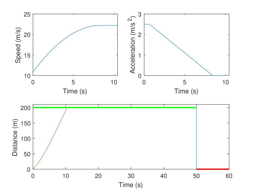
Figure 2: Case I in Table I with $v_{0}=10.8869$.

When the initial speed is relatively large, the vehicle should not start with full acceleration. This is the case shown in Fig. 3.

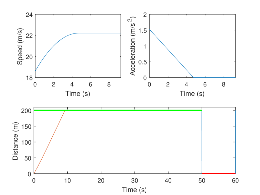
Figure 3: Case III in Table I with $v_{0}=18.6182$.

In the last two figures, the traffic light starts at a green state. The following two figures show the case when the traffic light starts at a red state. It can be inferred from the first two plots that the arrival time obtained from the free terminal time optimal control problem should be within the red light interval. Figure 4 shows a case when the initial speed is slow. The optimal arrival time obtained from the free terminal time optimal control is 12.1860 seconds. However, the traffic light in the first 40 seconds is red. The optimal time for the vehicle to arrive at the intersection is 40 seconds. The vehicle has adequate time to accelerate, therefore, it does not start with full acceleration, and it is unnecessary to accelerate to the maximum speed.

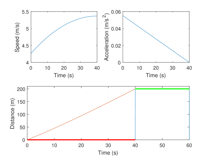
Figure 4: Case V in Table II with $v_{0}=4.2634$.

Figure 5 exhibits a different traffic light pattern, where the traffic light in the first 20 seconds is red. Due to a relatively large initial speed, the vehicle has to decelerate to cross the intersection when the traffic light is green.

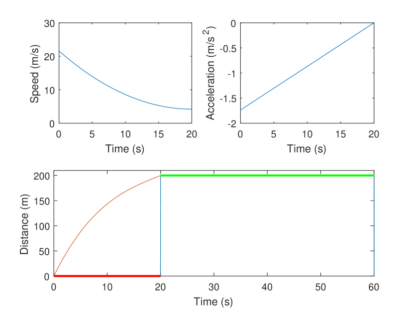
Figure 5: Case X in Table III with $v_{0}=21.5791$.

In the following, we test the optimal controller on a road of length $2203~{}m$. Due to this length, the optimal arrival time usually does not fall within the first green light cycle, and sometimes it is impossible for the vehicle to arrive at the traffic light within this cycle. For the case in Fig. 6, the optimal arrival time calculated from the free terminal time optimal control problem is 102.3476 seconds. Unfortunately, this arrival time belongs to a red light interval. Therefore, full acceleration is used to reach the speed limit and cross the intersection at 100 seconds when the traffic light is green.

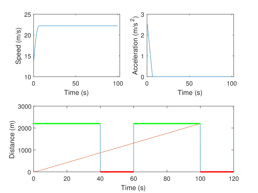
Figure 6: Case II in Table II with $v_{0}=13.4875$.

Figure 7 shows the case when the vehicle has a relatively fast initial speed compared to Fig. 6. Therefore, the vehicle does not start with full acceleration to reach the speed limit and catch the green light at 100 seconds.

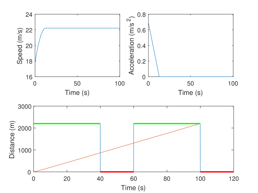
Figure 7: Case IV in Table II with $v_{0}=17.7745$.

For the last case in Fig. 8, the initial speed is very large. The best option is to decelerate the vehicle to cross the intersection at 120 seconds when the traffic light is green.

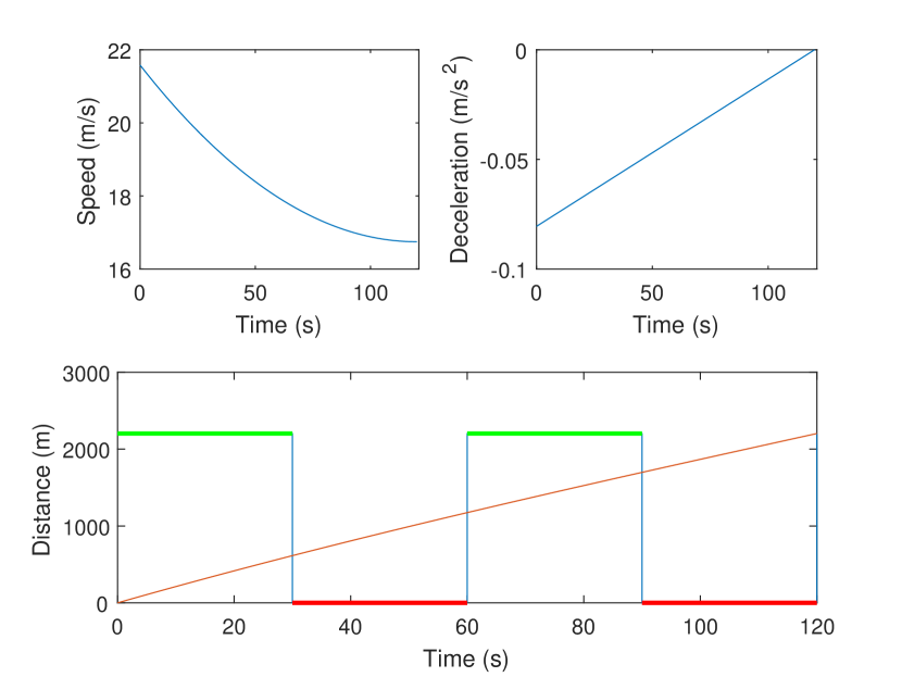
Figure 8: Case X in Table III with $v_{0}=21.5791$.

Exploring the time-energy tradeoff. In order to compare the performance between $(i)$ autonomous vehicles under the optimal control developed and $(ii)$ a human driver, we arbitrarily define the following rules as the driving behavior of a human driver:

• Full acceleration when the traffic light is green;

• No acceleration/deceleration when the traffic light is red.

We calculate the performance of both autonomous vehicles and human drivers for the different scenarios encountered from Fig. 2 to Fig. 8, and summarize the results in Table IV. The improvement is more than 10% for the case in Fig. 4. The performance improvement is calculated as the performance difference between the human driver and autonomous vehicle divided by the performance of the human driver. It is particularly challenging for a human driver to make a decision when he/she faces a steady red traffic light.

TABLE IV: Performance Comparison Between Human Driver (HD) and Autonomous Vehicle (AV)

	HD	AV	Improvement
Fig. 2	0.1611	0.1574	2.3%
Fig. 3	0.1294	0.1263	2.4%
Fig. 4	0.5965	0.5310	10.98%
Fig. 5	0.2655	0.2841	NA
Fig. 6	0.1300	0.1224	5.85%
Fig. 7	0.1406	0.1350	3.98%
Fig. 8	0.1461	0.1448	0.89%

Also note that the weighting parameter $\rho$ is chosen to be in favor of travel time rather than energy efficiency. Therefore, the performance improvement would be larger when we decrease the weighting parameter $\rho$, which provides a trade-off between energy consumption and travel time.

Figure 9 shows the travel time and the energy consumption when we vary the parameter $\rho$ from 0 to 1. The initial speed is chosen as $v_{0}=18.6182$. By exploring the trade-off curve, one may select am appropriate weight parameter $\rho$ depending on a particular application of interest. For instance, if energy efficiency is a major concern, Fig. 9 suggests to not select a large value for $\rho$ since the energy consumption grows rapidly as $\rho$ approaches $1$. On the other hand, a small $\rho$ is likely not a better option, since we can see that energy consumption does not significantly increase with $\rho$ increasing as long as $\rho<0.7$ (approximately). In fact, when $\rho$ increases from 0 to 0.7, the travel time is significantly reduced by $42.84\%$ whereas the energy consumption increases by only $4.85\%$. It is noteworthy that both curves show different trends around the circled area shown in Fig. 9: this is mainly because the optimal control has included the full acceleration part when the parameter $\rho$ is large.

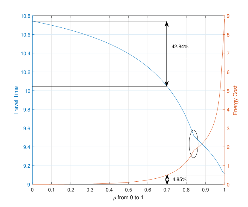
Figure 9: Trade-off between travel time and energy consumption

V Conclusions

This paper provided the optimal acceleration/deceleration profile for autonomous vehicles approaching an intersection based on the traffic light information, which could be obtained from an intelligent infrastructure via V2I communication. The solution for the above problem had the key feature of avoiding idling at a red light. Comparing with similar problems solved by numerical calculations, we provided a real-time analytical solution. The proposed algorithm offered better efficiency in terms of travel time and energy consumption, which has been verified through extensive simulations. The simulation results showed that the algorithm achieved substantial performance improvement compared with vehicles with heuristic human driver behavior.

There are a few avenues available for extending this work. In particular, there is a need to consider a practical scenario where interferences from other road users present. A possible way of doing this is to predict the driving behavior of vehicles ahead. It is also desirable to develop a more general algorithm by taking into account traffic light information at multiple intersections.

Appendix A Proof of Lemma 1

Let us first consider the case of constant control input. By solving the differential equation (2), it is straightforward to get the expression for $v\left(t_{1}\right)$. As a byproduct, we have $v\left(t\right)=v_{0}+\left(t-t_{0}\right)u$. By solving the differential equation (1), it follows that

$$x\left(t_{1}\right) =x_{0}+\int_{t_{0}}^{t_{1}}\left[v_{0}+\left(t-t_{0}\right)u\right]dt$$

$$=x_{0}+v_{0}\left(t_{1}-t_{0}\right)+\frac{1}{2}u\left(t_{1}-t_{0}\right)^{2}\text{.}$$

The energy consumption $J^{u}$ is then easy to obtain.

Next, let us consider the case that $u\left(t\right)=u\left(t_{1}-t\right)$ for $t\in\left[t_{0},t_{1}\right]$. Solving the differential equation (2), we obtain

$$v\left(t_{1}\right) =v_{0}+\int_{t_{0}}^{t_{1}}\left[u\left(t_{1}-t\right)\right]dt$$

$$=v_{0}+\frac{1}{2}u\left(t_{1}-t_{0}\right)^{2}.$$

As a byproduct, we have $v\left(t\right)=v_{0}+\frac{1}{2}u\left(t-t_{0}\right)^{2}$. Solving the differential equation (1) yields

$$x\left(t_{1}\right) =x_{0}+\int_{t_{0}}^{t_{1}}\left[v_{0}+\frac{1}{2}u\left(t-t_{0}\right)^{2}\right]dt$$

$$=x_{0}+v_{0}\left(t_{1}-t_{0}\right)+\frac{1}{6}u\left(t_{1}-t_{0}\right)^{3}\text{.}$$

The energy consumption is then calculated as

$$J^{u}=\int_{t_{0}}^{t_{1}}u^{2}\left(t_{1}-t\right)^{2}dt=\frac{1}{3}u^{2}\left(t_{1}-t_{0}\right)^{3}.$$

Appendix B Proof of Lemma 2

We will prove the result by a contradiction argument. Let us assume that $u^{\ast}\left(t\right)$ and $t_{p}^{\ast}$ are the optimal control and the optimal arrival time of Problem 2, respectively. In addition, we assume that there exists an interval $\left[t_{1},t_{2}\right]$ such that $u^{\ast}(t)<0$. Next, we construct another control input $u\left(t\right)$ such that $u\left(t\right)=u^{\ast}\left(t\right)$ for $t<t_{1}$, and $u\left(t\right)=0$ for $t\in\left[t_{1},t_{2}\right]$. It is then straightforward to get

$$v^{\ast}(t_{1})=v(t_{1}),\text{ and }x^{\ast}(t_{1})=x(t_{1}).$$

We now invoke the comparison lemma [22] which compares the solutions of the differential inequality $\dot{v}(t)\leq f(t,v)$ with the solution of the differential equation $\dot{u}(t)=f(t,u)$ and asserts that If $v_{0}\leq u_{0}$, then $v(t)\leq u(t)$. By applying the comparison principle to the dynamics of $v(t)$, it follows that

$$v^{\ast}(t)<v(t)$$ (51)

for $t>t_{1}$ until $v^{\ast}(t)=v_{\max}$. By applying the comparison principle again to the dynamics of $x(t)$, it follows that $x^{\ast}(t)<x(t)$ for $t>t_{1}$. Then, according to the terminal condition

$$x^{\ast}(t_{p})<x(t_{p})=l,$$

we conclude that $t_{p}^{\ast}>t_{p}$, therefore we have

$$t_{p}-t_{0}<t_{p}^{\ast}-t_{0}.$$ (52)

Let $\tau$ be the time when $v(\tau)=v_{\max}$, and we assume that $\tau>t_{2}$ without loss of generality. The remaining control input of $u(t)$ is thus constructed as

$$u\left(t\right)=\left\{\begin{array}[c]{ll}u^{\ast}\left(t\right)&\text{for }t_{2}\leq t<\min\left\{\tau,t_{p}\right\}\\ 0&\text{for }t\geq\min\left\{\tau,t_{p}\right\}.\end{array}\right.$$

By using the inequality (51) at $t=\tau$ we have

$$v^{\ast}(\tau)<v(\tau)=v_{\max}$$

Recalling that $u^{\ast}(t)<0$, $u\left(t\right)=0$ for $t\in\left[t_{1},t_{2}\right]$, it follows that

$$\int_{t_{0}}^{t_{p}}u^{2}\left(t\right)dt= \int_{t_{0}}^{t_{1}}u^{2}\left(t\right)dt+\int_{t_{2}}^{\min\left\{\tau,t_{p}\right\}}u^{2}\left(t\right)dt$$

$$< \int_{t_{0}}^{t_{1}}u^{\ast}\left(t\right)^{2}dt+\int_{t_{1}}^{t_{2}}u^{\ast}\left(t\right)^{2}dt$$

$$+\int_{t_{2}}^{\min\left\{\tau,t_{p}\right\}}u^{\ast}\left(t\right)^{2}dt$$

$$\leq \int_{t_{0}}^{t_{p}^{\ast}}u^{\ast}\left(t\right)^{2}dt.$$

The above inequality together with (52) contradicts the optimality of $u^{\ast}(t)$ and $t_{p}^{\ast}$ in (9) and completes the proof by contradiction. Therefore, we conclude tha $u^{\ast}(t)\geq 0$ for all $t\in[t_{0},t_{p}^{\ast}]$.

Appendix C Calculations for Table I

Let us assume that $\rho_{u}\neq 0$, and $\rho_{t}\neq 0$.

C-A Case I: $v^{*}\left(t_{p}^{\ast}\right)=v_{\max}$

Let us first find the time duration $\delta$ such that $u\left(t\right)$ decreases from $u_{\max}$ to $0$ while the speed increases from $v$ to the maximum speed $v_{\max}$ under the optimal control

$$\dot{u}\left(t\right)=-\frac{\rho_{t}}{2\rho_{u}v_{\max}}\text{.}$$ (53)

Integrating (53) on both sides yields

$$0=u_{\max}-\frac{\rho_{t}}{2\rho_{u}v_{\max}}\delta$$

which can be simplified as

$$\delta=2u_{\max}v_{\max}\frac{\rho_{u}}{\rho_{t}}.$$

According to Lemma 1, we know that

$$v_{\max}=v+u_{\max}^{2}v_{\max}\frac{\rho_{u}}{\rho_{t}},$$

which can be written as

$$v=\left(1-u_{\max}^{2}\frac{\rho_{u}}{\rho_{t}}\right)v_{\max}$$

with the assumption that

$$\left(1-u_{\max}^{2}\frac{\rho_{u}}{\rho_{t}}\right)v_{\max}\geq v_{\min}.$$

For the same amount of time, the distance that the vehicle travels is

$$d=2u_{\max}v_{\max}^{2}\frac{\rho_{u}}{\rho_{t}}-\frac{2}{3}u_{\max}^{3}v_{\max}^{2}\frac{\rho_{u}^{2}}{\rho_{t}^{2}}\text{.}$$

According to Theorem 1, the optimal control can be parameterized in terms of the speed $v(t)$ as

$$\left\{\begin{array}[c]{ll}u^{\ast}\left(t\right)=u_{\max}&\text{if }v\left(t\right)\leq\left(1-u_{\max}^{2}\frac{\rho_{u}}{\rho_{t}}\right)v_{\max}\\ \dot{u}^{\ast}\left(t\right)=\frac{-\rho_{t}}{2\rho_{u}v_{\max}}&\text{if }\left(1-u_{\max}^{2}\frac{\rho_{u}}{\rho_{t}}\right)v_{\max}\leq v\left(t\right)\leq v_{\max}\\ u^{\ast}\left(t\right)=0&\text{if }v\left(t\right)=v_{\max}\end{array}\right.$$

There are different cases depending on the relationship between the initial speed $v_{0}$ and the road length $l$. Remind that the analysis is under the assumption that

$$\left(1-u_{\max}^{2}\frac{\rho_{u}}{\rho_{t}}\right)v_{\max}\geq v_{\min}.$$

C-A1 Case I.1 $v_{0}\leq\left(1-u_{\max}^{2}\frac{\rho_{u}}{\rho_{t}}\right)v_{\max}$

(The first column in Table I). In this case, the vehicle will first accelerate to $v\left(t_{1}\right)=\left(1-u_{\max}^{2}\frac{\rho_{u}}{\rho_{t}}\right)v_{\max}$ using the maximum acceleration $u_{\max}$. Then it will travel a distance $d$ to reach $v_{\max}$. At time $t_{1}$, we have

$$x\left(t_{1}\right)=v_{0}\left(t_{1}-t_{0}\right)+\frac{1}{2}\left(t_{1}-t_{0}\right)^{2}u_{\max}\text{.}$$

It is easy to figure out that

$$t_{1}-t_{0}=\frac{\left(1-u_{\max}^{2}\frac{\rho_{u}}{\rho_{t}}\right)v_{\max}-v_{0}}{u_{\max}}\text{.}$$

To achieve the maximum speed $v_{\max}$, the road length $l$ must satisfy

$$l \geq x(t_{1})+d$$

$$=\frac{v_{\max}^{2}-v_{0}^{2}}{2u_{\max}}+u_{\max}v_{\max}^{2}\frac{\rho_{u}}{\rho_{t}}-\frac{1}{6}u_{\max}^{3}v_{\max}^{2}\frac{\rho_{u}^{2}}{\rho_{t}^{2}}.$$

C-A2 Case I.2 $\left(1-u_{\max}^{2}\frac{\rho_{u}}{\rho_{t}}\right)v_{\max}<v_{0}\leq v_{\max}$

(The third column in Table I). In this case, the vehicle will not start with full acceleration, and we have

$$u^{\ast}\left(t\right)=\frac{\rho_{t}}{2\rho_{u}}\frac{\tau-t}{v_{\max}},$$

where $\tau$ is the time when $v\left(\tau\right)=v_{\max}$.

According to Lemma 1, we can obtain

$$x\left(\tau\right) =v_{0}\left(\tau-t_{0}\right)+\frac{\rho_{t}}{6\rho_{u}v_{\max}}\left(\tau-t_{0}\right)^{3},$$

and

$$v_{\max}=v_{0}+\frac{\rho_{t}}{4\rho_{u}v_{\max}}\left(\tau-t_{0}\right)^{2}.$$ (54)

We can calculate from (54) to get

$$\tau-t_{0}=2\sqrt{\left(v_{\max}-v_{0}\right)v_{\max}\frac{\rho_{u}}{\rho_{t}}}.$$ (55)

By using (55), a necessary condition for $v\left(t\right)$ to reach the maximum speed $v_{\max}$ is

$$l \geq 2v_{0}\sqrt{\left(v_{\max}-v_{0}\right)v_{\max}\frac{\rho_{u}}{\rho_{t}}}$$

$$+\frac{4}{3}\left(v_{\max}-v_{0}\right)\sqrt{\left(v_{\max}-v_{0}\right)v_{\max}\frac{\rho_{u}}{\rho_{t}}}.$$ (56)

C-B Case II: $v^{*}\left(t_{p}^{\ast}\right)<v_{\max}$

C-B1 Case II.1 $v_{0}<\left(1-u_{\max}^{2}\frac{\rho_{u}}{\rho_{t}}\right)v_{\max}$

(The second column in Table I). In this case, the road length

$$l<\frac{v_{\max}^{2}-v_{0}^{2}}{2u_{\max}}+u_{\max}v_{\max}^{2}\frac{\rho_{u}}{\rho_{t}}-\frac{1}{6}u_{\max}^{3}v_{\max}^{2}\frac{\rho_{u}^{2}}{\rho_{t}^{2}}$$

is not long enough for the vehicle to reach the maximum speed. Let us assume that the speed when the acceleration starts to decrease at time $t_{1}$ is $v$. According to Lemma 1, it takes the time

$$t_{1}-t_{0}=\frac{v-v_{0}}{u_{\max}}$$

for the vehicle to reach the speed $v$ by using the maximum acceleration, and

$$x\left(t_{1}\right)=\frac{v^{2}-v_{0}^{2}}{2u_{\max}}\text{.}$$

The speed $v$ increases to $v^{\ast}\left(t_{p}^{\ast}\right)$ by using a linearly decreasing optimal control from $u_{\max}$ to $0$. It is easy to get that

$$\dot{u}\left(t\right)=-\frac{\rho_{t}}{2\rho_{u}v^{\ast}\left(t_{p}^{\ast}\right)}.$$

Therefore, the time for $u_{\max}$ to decrease to $0$ is

$$\delta_{2}=2u_{\max}v^{\ast}\left(t_{p}^{\ast}\right)\frac{\rho_{u}}{\rho_{t}}\text{.}$$

According to Lemma 1, we can obtain

$$v^{\ast}\left(t_{p}^{\ast}\right) =v+u_{\max}^{2}v^{\ast}\left(t_{p}^{\ast}\right)\frac{\rho_{u}}{\rho_{t}},$$

which is

$$v^{\ast}\left(t_{p}^{\ast}\right)=\frac{v}{1-\frac{\rho_{u}}{\rho_{t}}u_{\max}^{2}}.$$

By the road length constraint, we are able to calculate $v$ from the equality

$$l=\frac{v^{2}-v_{0}^{2}}{2u_{\max}}+v^{2}\frac{2u_{\max}}{1-\frac{\rho_{u}}{\rho_{t}}u_{\max}^{2}}\frac{\rho_{u}}{\rho_{t}}+\frac{4}{3}v^{2}\frac{\rho_{u}^{2}}{\rho_{t}^{2}}\frac{u_{\max}^{3}}{\left(1-\frac{\rho_{u}}{\rho_{t}}u_{\max}^{2}\right)^{2}},$$

that is,

$$v=\sqrt{\frac{2u_{\max}l+v_{0}^{2}}{1+\frac{4u_{\max}^{2}}{1-\frac{\rho_{u}}{\rho_{t}}u_{\max}^{2}}\frac{\rho_{u}}{\rho_{t}}+\frac{8}{3}\frac{u_{\max}^{4}}{\left(1-\frac{\rho_{u}}{\rho_{t}}u_{\max}^{2}\right)^{2}}\frac{\rho_{u}^{2}}{\rho_{t}^{2}}}}$$

C-B2 Case II.2 $v_{0}>\left(1-u_{\max}^{2}\frac{\rho_{u}}{\rho_{t}}\right)v_{\max}$

(The fourth column in Table I). In this case, the road length

$$l< \,2v_{0}\sqrt{\left(v_{\max}-v_{0}\right)v_{\max}\frac{\rho_{u}}{\rho_{t}}}$$

$$\quad+\frac{4}{3}\left(v_{\max}-v_{0}\right)\sqrt{\left(v_{\max}-v_{0}\right)v_{\max}\frac{\rho_{u}}{\rho_{t}}}$$

is not large enough for the vehicle to reach the speed limit, and the maximum acceleration $u_{\max}$ will not be used either. According to Theorem 1, the optimal control can be parameterized as

$$u^{\ast}\left(t\right)=\frac{\rho_{t}\left(t_{p}^{\ast}-t\right)}{2\rho_{u}v^{\ast}\left(t_{p}^{\ast}\right)}.$$

According to Lemma 1, we have

$$v^{\ast}\left(t_{p}^{\ast}\right)=v_{0}+\frac{\rho_{t}\left(t_{p}^{\ast}-t_{0}\right)^{2}}{4\rho_{u}v^{\ast}\left(t_{p}^{\ast}\right)},$$ (57)

and

$$l=v_{0}\left(t_{p}^{\ast}-t_{0}\right)+\frac{\rho_{t}}{6\rho_{u}v^{\ast}\left(t_{p}^{\ast}\right)}\left(t_{p}^{\ast}-t_{0}\right)^{3}.$$ (58)

By solving the equation (57), we can obtain

$$v^{*}(t_{p}^{*})=\frac{v_{0}+\sqrt{v_{0}^{2}+\frac{\rho_{t}}{\rho_{u}}\left(t_{p}^{\ast}-t_{0}\right)^{2}}}{2}.$$

By substituting for $v^{*}(t_{p}^{*})$, we are able to obtain $t_{p}^{*}$ from (58).

Appendix D Detailed Calculations for Table II

There are different cases depending on the initial speed $v_{0}$, the time duration $kT+DT$, and the road length $l$.

D-A Case I: $u^{*}_{0}=u_{\max}$ and $\dot{u}^{*}\left(t\right)=0$

This case corresponds to $h(v_{0})=0$. The vehicle accelerates fully until it arrives at the traffic light or the maximum speed is reached. According to Lemma 1, the vehicle reaches the maximum speed by spending time

$$\delta=\frac{v_{\max}-v_{0}}{u_{\max}}.$$

Depending on the values of $kT+DT$ and $\delta$, we have different energy consumptions

$$J_{1}^{u}=\left\{\begin{array}[c]{cc}u_{\max}\left(v_{\max}-v_{0}\right)&\text{if }\frac{v_{\max}-v_{0}}{u_{\max}}<kT+DT\\ u_{\max}^{2}\left(kT+DT-t_{0}\right)&\text{if }\frac{v_{\max}-v_{0}}{u_{\max}}\geq kT+DT\end{array}\right.$$

For all other cases, $h\left(v_{0}\right)>0$, and $\dot{u}\left(t\right)\neq 0$ for some $t$.

D-B Case II: $u^{\ast}\left(t_{0}\right)=u_{\max}$, and $v^{\ast}\left(t_{p}\right)=v_{\max}$

The time $t_{1}$ is when the acceleration starts to decrease, that is,

$$\frac{1}{2}\frac{u_{\max}^{2}\left(\tau-t_{1}\right)}{v_{0}-v_{\max}+\left(\tau-t_{0}\right)u_{\max}}=u_{\max}.$$ (59)

From (59), we can obtain

$$\tau=2\frac{v_{\max}-v_{0}}{u_{\max}}-t_{1}+2t_{0}\text{.}$$

According to Lemma 1,

$$v\left(t_{1}\right) =v_{0}+u_{\max}\left(t_{1}-t_{0}\right)$$

$$x\left(t_{1}\right) =v_{0}\left(t_{1}-t_{0}\right)+\frac{1}{2}u_{\max}\left(t_{1}-t_{0}\right)^{2}$$

and

$$x\left(\tau\right)=x\left(t_{1}\right)+v\left(t_{1}\right)\left(\tau-t_{1}\right)+\frac{1}{6}\frac{u_{\max}^{2}\left(\tau-t_{1}\right)^{3}}{v_{0}-v_{\max}+\left(\tau-t_{0}\right)u_{\max}}.$$

Therefore, we have

$$l=\left(t_{p}-\tau\right)v_{\max}+x\left(\tau\right).$$ (60)

We can solve the equation (60) to get $t_{1}$. The energy consumption can be expressed as

$$J_{2}^{u}=\left(t_{1}-t_{0}\right)u_{\max}^{2}+\frac{1}{12}\frac{u_{\max}^{4}\left(\tau-t_{1}\right)^{3}}{\left[v_{0}-v_{\max}+\left(\tau-t_{0}\right)u_{\max}\right]^{2}}.$$

D-C Case III: $u^{\ast}\left(t_{0}\right)=u_{\max}$, and $v^{\ast}\left(t_{p}\right)<v_{\max}$

In this case, $\tau=t_{p}$. First, we need to find the time $t_{1}$ such that the acceleration starts to decrease, that is,

$$\frac{1}{2}\frac{u_{\max}^{2}\left(t_{p}-t_{1}\right)}{v_{0}-v^{\ast}\left(t_{p}\right)+\left(t_{p}-t_{0}\right)u_{\max}}=u_{\max}\text{.}$$

By solving the above equation for $v^{\ast}\left(t_{p}\right)$, we can obtain

$$v^{\ast}\left(t_{p}\right)=v_{0}+\frac{t_{p}+t_{1}-2t_{0}}{2}u_{\max}\text{.}$$ (61)

According to Lemma 1, the speed and the distance of the vehicle at $t_{1}$ are

$$v^{*}\left(t_{1}\right)=v_{0}+\left(t_{1}-t_{0}\right)u_{\max},$$

and

$$x^{*}\left(t_{1}\right)=v_{0}\left(t_{1}-t_{0}\right)+\frac{1}{2}u_{\max}\left(t_{1}-t_{0}\right)^{2},$$

respectively. From the road length constraint

$$l=x^{*}\left(t_{1}\right)+v^{*}\left(t_{1}\right)\left(t_{p}-t_{1}\right)+\frac{1}{3}u_{\max}\left(t_{p}-t_{1}\right)^{2},$$ (62)

we are able to calculate $t_{1}$. The energy consumption for this case can be expressed as

$$J_{3}^{u}=\frac{u_{\max}^{2}\left(t_{p}+2t_{1}-3t_{0}\right)}{3}\text{.}$$

D-D Case IV $u_{0}^{\ast}<u_{\max}$ and $v^{\ast}\left(t_{p}\right)=v_{\max}$

In this case, the vehicle reaches the maximum speed at $\tau$. According to Lemma 1, we have

$$v_{\max}=v_{0}+\frac{1}{4}\frac{u^{\ast}\left(t_{0}\right)^{2}\left(\tau-t_{0}\right)^{2}}{v_{0}-v_{\max}+\left(\tau-t_{0}\right)u^{\ast}\left(t_{0}\right)}\text{,}$$ (63)

Solving the above equation for $u^{\ast}\left(t_{0}\right)$ yields

$$u^{\ast}\left(t_{0}\right)=2\frac{v_{\max}-v_{0}}{\tau-t_{0}}.$$

With the expression of $u^{\ast}\left(t_{0}\right)$ and Lemma 1, we can obtain

$$l=\frac{1}{3}\left(v_{0}+2v_{\max}\right)\left(\tau-t_{0}\right)+\left(t_{p}-\tau\right)v_{\max}\text{.}$$ (64)

We can calculate $\tau$ from (64) as

$$\tau=\frac{3l+\left(2v_{\max}+v_{0}\right)t_{0}-3t_{p}v_{\max}}{v_{0}-v_{\max}}\text{.}$$

The energy consumption in this case is expressed as

$$J_{4}^{u}=\frac{4}{3}\frac{\left(v_{\max}-v_{0}\right)^{2}}{\tau-t_{0}}\text{.}$$

D-E Case V: $u_{0}^{\ast}<u_{\max}$ and $v^{\ast}\left(t_{p}\right)<v_{\max}$

In this case, $\tau=t_{f}$. According to Lemma 1, the final speed is

$$v^{\ast}\left(t_{p}\right)=v_{0}+\frac{1}{4}\frac{u^{\ast}\left(t_{0}\right)^{2}\left(t_{p}-t_{0}\right)^{2}}{v_{0}-v^{\ast}\left(t_{p}\right)+\left(t_{p}-t_{0}\right)u^{\ast}\left(t_{0}\right)},$$ (65)

From (65), we can get

$$u^{\ast}\left(t_{0}\right)=2\frac{v^{\ast}\left(t_{p}\right)-v_{0}}{t_{p}-t_{0}}\text{.}$$

Using the expression of $u^{\ast}\left(t_{0}\right)$ and Lemma 1, we can obtain

$$l=v_{0}\left(t_{p}-t_{0}\right)+\frac{2}{3}\left(v^{\ast}\left(t_{p}\right)-v_{0}\right)\left(t_{p}-t_{0}\right)\text{.}$$ (66)

Solving the equation (66), we have

$$v^{\ast}\left(t_{p}\right)=\frac{3}{2}\frac{l-v_{0}\left(t_{p}-t_{0}\right)}{t_{p}-t_{0}}+v_{0}\text{.}$$

The energy consumption in this case can be expressed as

$$J_{5}^{u}=3\frac{\left[l-v_{0}\left(t_{p}-t_{0}\right)\right]^{2}}{\left(t_{p}-t_{0}\right)^{3}}.$$

Appendix E Detailed Calculations for Table III

E-A Case VII: $u\left(t_{0}\right)=u_{\min}$ and $v\left(t_{p}\right)=v_{\min}$.

In this case, the vehicle starts with full deceleration $u_{\min}$, and then at time $t_{1},$ the deceleration linearly increases until it reaches zero at $t=\tau$. Therefore, at time $t=t_{1}$, we have

$$u_{\min}=\frac{1}{2}\frac{u_{\min}^{2}\left(\tau-t_{1}\right)}{v_{0}+\left(\tau-t_{0}\right)u_{\min}-v_{\min}},$$

that is,

$$v_{0}-v_{\min}=\frac{2t_{0}-\tau-t_{1}}{2}u_{\min}.$$ (67)

According to Lemma 1, the speed and travel distance of the vehicle at time $t_{1}$ are

$$v\left(t_{1}\right)=v_{0}+u_{\min}\left(t_{1}-t_{0}\right),$$

and

$$x\left(t_{1}\right)=v_{0}\left(t_{1}-t_{0}\right)+\frac{1}{2}u_{\min}\left(t_{1}-t_{0}\right)^{2},$$

respectively. At time $\tau,$ we have

$$x\left(\tau\right)=x\left(t_{1}\right)+v\left(t_{1}\right)\left(\tau-t_{1}\right)+\frac{1}{6}\frac{u_{\min}^{2}\left(\tau-t_{1}\right)^{3}}{v_{0}+\left(\tau-t_{0}\right)u_{\min}-v_{\min}}$$

To satisfy the road length constraint, we must have

$$l=x\left(\tau\right)+\left(kT+T-\tau\right)v_{\min}\text{.}$$ (68)

We can solve (67) to obtain

$$\tau=2t_{0}-t_{1}+2\frac{v_{\min}-v_{0}}{u_{\min}}$$

and (68) to get $t_{1}$. The energy consumption in this case can be expressed as

$$J_{7}^{u}=\left(t_{1}-t_{0}\right)u_{\min}^{2}+\frac{1}{12}\frac{u_{\min}^{4}\left(\tau-t_{1}\right)^{3}}{\left[v_{0}+\left(\tau-t_{0}\right)u_{\min}-v_{\min}\right]^{2}}.$$

E-B Case VIII: $u^{\ast}\left(t_{0}\right)=u_{\min}$ and $v^{\ast}\left(t_{p}\right)>v_{\min}$.

In this case, $\tau=t_{f}$. The vehicle starts with full deceleration $u_{\min}$, and at time $t_{1}$, the deceleration starts to increase. Similarly, we have

$$v_{0}-v^{\ast}\left(t_{p}\right)=\frac{2t_{0}-t_{p}-t_{1}}{2}u_{\min}.$$ (69)

According to Lemma 1, we know that

$$v^{\ast}\left(t_{1}\right) =v_{0}+u_{\min}\left(t_{1}-t_{0}\right),$$

$$x^{\ast}\left(t_{1}\right) =v_{0}\left(t_{1}-t_{0}\right)+\frac{1}{2}u_{\min}\left(t_{1}-t_{0}\right)^{2}.$$

Solving (69), we can get

$$v^{\ast}\left(t_{p}\right)=v_{0}+\frac{t_{1}+t_{p}-2t_{0}}{2}u_{\min}\text{.}$$

Using the expression of $v^{\ast}\left(t_{p}\right)$, we can obtain $t_{1}$ by solving the following equation

$$l=x^{\ast}\left(t_{1}\right)+v^{\ast}\left(t_{1}\right)\left(t_{p}-t_{1}\right)+\frac{1}{3}u_{\min}\left(t_{p}-t_{1}\right)^{2}.$$ (70)

The energy consumption in this case can be expressed as

$$J_{8}^{u}=\frac{u_{\min}^{2}\left(t_{p}+2t_{1}-3t_{0}\right)}{3}.$$

E-C Case IX: $u^{\ast}\left(t_{0}\right)<u_{\min}$, and $v^{\ast}\left(t_{p}\right)=v_{\min}$.

In this case, the vehicle starts with linearly increasing deceleration until it reaches the minimum speed $v_{\min}$.

According to Lemma 1, we have

$$v_{\min}=v_{0}+\frac{1}{4}\frac{u^{\ast}\left(t_{0}\right)^{2}\left(\tau-t_{0}\right)^{2}}{v_{0}+\left(\tau-t_{0}\right)u^{\ast}\left(t_{0}\right)-v_{\min}}.$$ (71)

Solving $u^{\ast}\left(t_{0}\right)$ in (71) yields

$$u^{\ast}\left(t_{0}\right)=2\frac{v_{\min}-v_{0}}{\tau-t_{0}}\text{.}$$

According to Lemma 1 and the expression of $u^{\ast}\left(t_{0}\right)$, the distance of the vehicle at time $\tau$ is given as

$$x\left(\tau\right)=\frac{1}{3}\left(2v_{\min}+v_{0}\right)\left(\tau-t_{0}\right).$$

Then, we can solve $\tau$ from the following equation

$$l=x\left(\tau\right)+\left(KT+T-\tau\right)v_{\min}\text{,}$$ (72)

that is,

$$\tau=\frac{3l+\left(2v_{\min}+v_{0}\right)t_{0}-3t_{p}v_{\min}}{v_{0}-v_{\min}}.$$

The energy consumption in this case can be expressed as

$$J_{9}^{u}=\frac{4}{3}\frac{\left(v_{\min}-v_{0}\right)^{2}}{\tau-t_{0}}.$$

E-D Case X: $u^{\ast}\left(t_{0}\right)<u_{\min}$, and $v^{\ast}\left(t_{p}\right)<v_{\min}$.

In this case, $\tau=t_{p}$. The optimal control only contains the linear increasing deceleration process. According to Lemma 1, we have

$$v^{\ast}\left(t_{p}\right)=v_{0}+\frac{1}{4}\frac{u^{\ast}\left(t_{0}\right)^{2}\left(t_{p}-t_{0}\right)^{2}}{v_{0}+\left(t_{p}-t_{0}\right)u^{\ast}\left(t_{0}\right)-v\left(t_{p}\right)},$$ (73)

$$l=v_{0}\left(t_{p}-t_{0}\right)+\frac{1}{6}\frac{u^{\ast}\left(t_{0}\right)^{2}\left(t_{p}-t_{0}\right)^{3}}{v_{0}+\left(t_{p}-t_{0}\right)u^{\ast}\left(t_{0}\right)-v^{\ast}\left(t_{p}\right)}.$$ (74)

We can solve $u^{\ast}\left(t_{0}\right)$ and $v^{\ast}\left(t_{p}\right)$ from (73) and (74) to obtain

$$u^{\ast}\left(t_{0}\right)=2\frac{v^{\ast}\left(t_{p}\right)-v_{0}}{t_{p}-v_{0}},$$

and

$$v^{\ast}\left(t_{p}\right)=\frac{3}{2}\frac{l-v_{0}\left(t_{p}-t_{0}\right)}{t_{p}-t_{0}}+v_{0}.$$

The energy consumption in this case is

$$J_{10}^{u}=3\frac{\left[l-v_{0}\left(t_{p}-t_{0}\right)\right]^{2}}{\left(t_{p}-t_{0}\right)^{3}}.$$

References

- [1] D. Schrank, B. Eisele, T. Lomax, and J. Bak, “2015 urban mobility scorecard,” Texas A&M Transportation Institute and INRIX, Tech. Rep., 2015.
- [2] L. Li, D. Wen, and D. Yao, “A survey of traffic control with vehicular communications,” IEEE Trans. Intell. Transport. Syst., vol. 15, no. 1, pp. 425–432, 2014.
- [3] E. G. Gilbert, “Vehicle cruise: Improved fuel economy by periodic control,” Automatica, vol. 12, no. 2, pp. 159 – 166, 1976.
- [4] J. Hooker, “Optimal driving for single-vehicle fuel economy,” Transportation Research Part A: General, vol. 22, no. 3, pp. 183 – 201, 1988.
- [5] E. Hellstrom, J. Aslund, and L. Nielsen, “Design of an efficient algorithm for fuel-optimal look-ahead control,” Control Engineering Practice, vol. 18, no. 11, pp. 1318 – 1327, 2010.
- [6] S. E. Li, H. Peng, K. Li, and J. Wang, “Minimum fuel control strategy in automated car-following scenarios,” IEEE Transactions on Vehicular Technology, vol. 61, no. 3, pp. 998–1007, 2012.
- [7] J. L. Fleck, C. G. Cassandras, and Y. Geng, “Adaptive quasi-dynamic traffic light control,” IEEE Trans. Control Syst. Technol., vol. 24, no. 3, pp. 830–842, 2016.
- [8] V. Milanes, J. Perez, E. Onieva, and C. Gonzalez, “Controller for urban intersections based on wireless communications and fuzzy logic,” IEEE Trans. Intell. Transport. Syst., vol. 11, no. 1, pp. 243–248, 2010.
- [9] J. Alonso, V. Milan s, J. P rez, E. Onieva, C. Gonz lez, and T. de Pedro, “Autonomous vehicle control systems for safe crossroads,” Transportation Research Part C: Emerging Technologies, vol. 19, no. 6, pp. 1095 – 1110, 2011.
- [10] S. Huang, A. W. Sadek, and Y. Zhao, “Assessing the mobility and environmental benefits of reservation-based intelligent intersections using an integrated simulator,” IEEE Trans. Intell. Transport. Syst., vol. 13, no. 3, pp. 1201–1214, 2012.
- [11] K. D. Kim and P. R. Kumar, “An mpc-based approach to provable system-wide safety and liveness of autonomous ground traffic,” IEEE Trans. Autom. Control, vol. 59, no. 12, pp. 3341–3356, 2014.
- [12] Y. J. Zhang, A. A. Malikopoulos, and C. G. Cassandras, “Optimal control and coordination of connected and automated vehicles at urban traffic intersections,” in Proc. of the 2016 American Control Conference, 2016, pp. 6227–6232.
- [13] J. Rios-Torres and A. A. Malikopoulos, “A survey on the coordination of connected and automated vehicles at intersections and merging at highway on-ramps,” IEEE Trans. Intell. Transport. Syst., vol. 18, no. 5, pp. 1066–1077, 2017.
- [14] http://www.audi.com/en/innovation/connect/smart-city.html.
- [15] B. Asadi and A. Vahidi, “Predictive cruise control: Utilizing upcoming traffic signal information for improving fuel economy and reducing trip time,” IEEE Trans. Control Syst. Technol., vol. 19, no. 3, pp. 707–714, 2011.
- [16] M. A. S. Kamal, M. Mukai, J. Murata, and T. Kawabe, “Model predictive control of vehicles on urban roads for improved fuel economy,” IEEE Transactions on Control Systems Technology, vol. 21, no. 3, pp. 831–841, 2013.
- [17] G. Mahler and A. Vahidi, “An optimal velocity-planning scheme for vehicle energy efficiency through probabilistic prediction of traffic-signal timing,” IEEE Trans. Intell. Transport. Syst., vol. 15, no. 6, pp. 2516–2523, 2014.
- [18] N. Wan, A. Vahidi, and A. Luckow, “Optimal speed advisory for connected vehicles in arterial roads and the impact on mixed traffic,” Transportation Research Part C: Emerging Technologies, vol. 69, pp. 548 – 563, 2016.
- [19] G. De Nunzio, C. Canudas de Wit, P. Moulin, and D. Di Domenico, “Eco-driving in urban traffic networks using traffic signals information,” International Journal of Robust and Nonlinear Control, vol. 26, no. 6, pp. 1307–1324, 2016.
- [20] R. F. Hartl, S. P. Sethi, and R. G. Vickson, “A survey of the maximum principles for optimal control problems with state constraints,” SIAM Review, vol. 37, no. 2, pp. 181–218, 1995.
- [21] A. Malikopoulos, “Real-Time, Self-Learning Identification and Stochastic Optimal Control of Advanced Powertrain Systems,” Ph.D. dissertation, The University of Michigan, 2008.
- [22] H. K. Khalil, Nonlinear Systems, 3rd ed. Prentice Hall, 2002.