ADMM for Multiaffine Constrained Optimization

Abstract.

We expand the scope of the alternating direction method of multipliers (ADMM). Specifically, we show that ADMM, when employed to solve problems with multiaffine constraints that satisfy certain verifiable assumptions, converges to the set of constrained stationary points if the penalty parameter in the augmented Lagrangian is sufficiently large. When the Kurdyka-Łojasiewicz (K-Ł) property holds, this is strengthened to convergence to a single constrained stationary point. Our analysis applies under assumptions that we have endeavored to make as weak as possible. It applies to problems that involve nonconvex and/or nonsmooth objective terms, in addition to the multiaffine constraints that can involve multiple (three or more) blocks of variables. To illustrate the applicability of our results, we describe examples including nonnegative matrix factorization, sparse learning, risk parity portfolio selection, nonconvex formulations of convex problems, and neural network training. In each case, our ADMM approach encounters only subproblems that have closed-form solutions.

1. Introduction

The alternating direction method of multipliers (ADMM) is an iterative method which, in its original form, solves linearly-constrained separable optimization problems with the following structure:

$$(P0)\hskip 15.00002pt\left\{\begin{array}[]{rll}\inf\limits_{x,y}&f(x)+g(y)\\ &Ax+By-b=0.\end{array}\right.$$

The augmented Lagrangian $\mathcal{L}$ of the problem $(P0)$, for some penalty parameter $\rho>0$, is defined to be

$$\mathcal{L}(x,y,w)=f(x)+g(y)+\langle w,Ax+By-b\rangle+\frac{\rho}{2}\|Ax+By-b\|^{2}.$$

In iteration $k$, with the iterate $({x}^{k},{y}^{k},{w}^{k})$, ADMM takes the following steps:

1. Minimize $\mathcal{L}(x,{y}^{k},{w}^{k})$ with respect to $x$ to obtain ${x}^{k+1}$.

2. Minimize $\mathcal{L}({x}^{k+1},y,{w}^{k})$ with respect to $y$ to obtain ${y}^{k+1}$.

3. Set ${w}^{k+1}\leftarrow{w}^{k}+\rho(A{x}^{k+1}+B{y}^{k+1}-b)$.

ADMM was first proposed [20, 21] for solving variational problems, and was subsequently applied to convex optimization problems with two blocks as in $(P0)$. Several techniques can be used to analyze this case, including an operator-splitting approach [16, 41]. The survey articles [17, 6] provide convergence proofs from several viewpoints, and discuss numerous applications of ADMM. More recently, there has been considerable interest in extending ADMM convergence guarantees when solving problems with multiple blocks and nonconvex objective functions. ADMM directly extends to the problem

$$(P1)\hskip 15.00002pt\left\{\begin{array}[]{rll}\inf\limits_{x_{1},x_{2},\ldots,x_{n}}&f_{1}(x_{1})+f_{2}(x_{2})+\ldots+f_{n}(x_{n})\\ &A_{1}x_{1}+A_{2}x_{2}+\ldots+A_{n}x_{n}-b=0\end{array}\right.$$

by minimizing $\mathcal{L}(x_{1},\ldots,x_{n},w)$ with respect to $x_{1},x_{2},\ldots,x_{n}$ successively. The multiblock problem turns out to be significantly different from the classical 2-block problem, even when the objective function is convex; for example, [9] exhibits an example with $n=3$ blocks and $f_{1},f_{2},f_{3}\equiv 0$ for which ADMM diverges for any value of $\rho$. Under certain conditions, the unmodified 3-block ADMM does converge. In [39], it is shown that if $f_{3}$ is strongly convex with condition number $\kappa\in[1,1.0798)$ (among other assumptions), then 3-block ADMM is globally convergent. If $f_{1},\ldots,f_{n}$ are all strongly convex, and $\rho>0$ is sufficiently small, then [24] shows that multiblock ADMM is convergent. Other works along these lines include [37, 38, 34].

In the absence of strong convexity, modified versions of ADMM have been proposed that can accommodate multiple blocks. In [13] a new type of 3-operator splitting is introduced that yields a convergent 3-block ADMM (see also [46] for a proof that a ‘lifting-free’ 3-operator extension of Douglas-Rachford splitting does not exist). Convergence guarantees for multiblock ADMM can also be achieved through variants such as proximal ADMM, majorized ADMM, linearized ADMM [49, 36, 14, 10, 40, 5], and proximal Jacobi ADMM [14, 55, 52].

ADMM has also been extended to problems with nonconvex objective functions. In [25], it is proved that ADMM converges when the problem $(P1)$ is either a nonconvex consensus or sharing problem, and [57] proves convergence under more general conditions on $f_{1},\ldots,f_{n}$ and $A_{1},\ldots,A_{n}$. Proximal ADMM schemes for nonconvex, nonsmooth problems are considered in [33, 60, 28, 5]. More references on nonconvex ADMM, and comparisons of the assumptions used, can be found in [57].

In all of the work mentioned above, the system of constraints $C(x_{1},\ldots,x_{n})=0$ is assumed to be linear. Consequently, when all variables other than $x_{i}$ have fixed values, $C(x_{1},\ldots,x_{n})$ becomes an affine function of $x_{i}$. However, this holds for more general constraints $C(\cdot)$ in the much larger class of multiaffine maps (see Section 2). Thus, it seems reasonable to expect that ADMM would behave similarly when the constraints $C(x_{1},\ldots,x_{n})=0$ are permitted to be multiaffine. To be precise, consider a more general problem than $(P1)$ of the form

$$(P2)\hskip 15.00002pt\left\{\begin{array}[]{rll}\inf\limits_{x_{1},x_{2},\ldots,x_{n}}&f(x_{1},\ldots,x_{n})\\ &C(x_{1},\ldots,x_{n})=0.\end{array}\right.$$

The augmented Lagrangian for $(P2)$ is

$$\mathcal{L}(x_{1},\ldots,x_{n},w)=f(x_{1},\ldots,x_{n})+\langle w,C(x_{1},\ldots,x_{n})\rangle+\frac{\rho}{2}\|C(x_{1},\ldots,x_{n})\|^{2},$$

and ADMM for solving this problem is specified in Algorithm 1.

Algorithm 1 ADMM

  Input: $(x_{1}^{0},\ldots,x_{n}^{0}),w^{0},\rho$

  for $k=0,1,2,\ldots$ do

     for $i=1,\ldots,n$ do

        Compute ${x}^{k+1}_{i}\in\operatorname{argmin}_{x_{i}}\mathcal{L}({x}^{k+1}_{1},\ldots,{x}^{k+1}_{i-1},x_{i},{x}^{k}_{i+1},\ldots,{x}^{k}_{n},{w}^{k})$

     end for

     ${w}^{k+1}\leftarrow{w}^{k}+\rho C({x}^{k+1}_{1},\ldots,{x}^{k+1}_{n})$

  end for

While many problems can be modeled with multiaffine constraints, existing work on ADMM for solving multiaffine constrained problems appears to be limited. Boyd et al. [6] propose solving the nonnegative matrix factorization problem formulated as a problem with biaffine constraints, i.e.,

$$(\text{NMF1})\hskip 15.00002pt\left\{\begin{array}[]{rll}\inf\limits_{Z,X,Y}&\frac{1}{2}\|Z-B\|^{2}\\ &Z=XY,X\geq 0,Y\geq 0,\end{array}\right.$$

by applying ADMM with alternating minimization on the blocks $Y$ and $(X,Z)$. The convergence of ADMM employed to solve the (NMF1) problem appears to have been an open question until a proof was given in [23]. A method derived from ADMM has also been proposed for optimizing a biaffine model for training deep neural networks [53]. For general nonlinear constraints, a framework for “monitored” Lagrangian-based multiplier methods was studied in [4].

In this paper, we establish the convergence of ADMM for a broad class of problems with multiaffine constraints. Our assumptions are similar to those used in [57] for nonconvex ADMM; in particular, we do not make any assumption about the iterates generated by the algorithm. Hence, these results extend the applicability of ADMM to a larger class of problems which naturally have multiaffine constraints. Moreover, we prove several results about ADMM in Section 6 that hold in even more generality, and thus may be useful for analyzing ADMM beyond the setting considered here.

1.1. Organization of this paper

In Section 2, we define multilinear and multiaffine maps, and specify the precise structure of the problems that we consider. In Section 3, we provide several examples of problems that can be formulated with multiaffine constraints. In Section 4, we state our assumptions and main results (i.e., Theorems 4.1, 4.3 and 4.5). In Section 5, we present a collection of necessary technical material. In Section 6, we prove several results about ADMM that hold under weak conditions on the objective function and constraints. Finally, in Section 7, we complete the proof of our main convergence theorems (Theorems 4.1, 4.3 and 4.5), by applying the general techniques developed in Section 6. Appendix A contains proofs of technical lemmas. Appendix B presents an alternative biaffine formulation for deep neural network training. Appendix C organizes the major assumptions in tabular form. Appendix D presents additional formulations of problems where all ADMM subproblems have closed-form solutions. Appendix E presents several numerical experiments.

1.2. Notation and Definitions

We consider only finite-dimensional real vector spaces. The symbols $\mathbb{E},\mathbb{E}_{1},\ldots,\mathbb{E}_{n}$ denote finite-dimensional Hilbert spaces, equipped with inner products $\langle\cdot,\cdot\rangle$. By default, we use the standard inner product on $\mathbb{R}^{n}$ and the trace inner product $\langle X,Y\rangle=\operatorname{Tr}(Y^{T}X)$ on the matrix space. Unless otherwise specified, the norm $\|\cdot\|$ is always the induced norm of the inner product. When $A$ is a matrix or linear map, $\|A\|_{op}$ denotes the $L_{2}$ operator norm, and $\|A\|_{*}$ denotes the nuclear norm (the sum of the singular values of $A$). Fixed bases are assumed, so we freely use various properties of a linear map $A$ that depend on its representation (such as $\|A\|_{op}$), and view $A$ as a matrix as required.

For $f:\mathbb{R}^{n}\rightarrow\mathbb{R}\cup\{\infty\}$, the effective domain $\operatorname{dom}(f)$ is the set $\{x:f(x)<\infty\}$. The image of a function $f$ is denoted by $\operatorname{Im}(f)$. Similarly, when $A$ is a linear map represented by a matrix, $\operatorname{Im}(A)$ is the column space of $A$. We use $\operatorname{Null}(A)$ to denote the null space of $A$. The orthogonal complement of a linear subspace $U$ is denoted $U^{\perp}$.

To distinguish the derivatives of smooth (i.e., continuously differentiable) functions from subgradients, we use the notation $\nabla_{X}$ for partial differentiation with respect to $X$, and reserve the symbol $\partial$ for the set of general subgradients (Section 5.1); hence, the use of $\nabla f$ serves as a reminder that $f$ is assumed to be smooth. A function $f$ is Lipschitz differentiable if it is differentiable and its gradient is Lipschitz continuous.

When $\mathcal{X}$ is a tuple of variables $\mathcal{X}=(X_{0},\ldots,X_{n})$, we write $\mathcal{X}_{\neq\ell}$ for $(X_{i}:i\neq\ell)$. Similarly, $\mathcal{X}_{>\ell}$ and $\mathcal{X}_{<\ell}$ represent $(X_{i}:i>\ell)$ and $(X_{i}:i<\ell)$ respectively.

We use the term constrained stationary point for a point satisfying necessary first-order optimality conditions; this is a generalization of the Karush-Kuhn-Tucker (KKT) necessary conditions to nonsmooth problems. For the problem $\min_{x}\{f(x):C(x)=0\}$, where $C$ is smooth and $f$ possesses general subgradients, $x^{\ast}$ is a constrained stationary point if $C(x^{\ast})=0$ and there exists $w^{\ast}$ with $0\in\partial f(x^{\ast})+\nabla C(x^{\ast})^{T}w^{\ast}$.

2. Multiaffine Constrained Problems

The central objects of this paper are multilinear and multiaffine maps, which generalize linear and affine maps.

Definition 2.1.

A map $\mathcal{M}:\mathbb{E}_{1}\oplus\ldots\oplus\mathbb{E}_{n}\rightarrow\mathbb{E}$ is multilinear if, for all $i\leq n$ and all points $(\overline{X}_{1},\ldots,\overline{X}_{i-1},\overline{X}_{i+1},\ldots,\overline{X}_{n})\in\bigoplus_{j\neq i}E_{j}$, the map $\mathcal{M}_{i}:\mathbb{E}_{i}\rightarrow\mathbb{E}$ given by

$$X_{i}\mapsto\mathcal{M}(\overline{X}_{1},\ldots,\overline{X}_{i-1},X_{i},\overline{X}_{i+1},\ldots,\overline{X}_{n})$$

is linear. Similarly, $\mathcal{M}$ is multiaffine if the map $\mathcal{M}_{i}$ is affine for all $i$ and all points of $\bigoplus_{j\neq i}\mathbb{E}_{j}$. In particular, when $n=2$, we say that $\mathcal{M}$ is bilinear/biaffine.

We consider the convergence of ADMM for problems of the form:

$$(P)\hskip 15.00002pt\left\{\begin{array}[]{rll}\displaystyle\inf_{\mathcal{X},\mathcal{Z}}&\phi(\mathcal{X},\mathcal{Z})\\ &A(\mathcal{X},Z_{0})+Q(\mathcal{Z}_{>})=0,\end{array}\right.$$

where $\mathcal{X}=(X_{0},\ldots,X_{n})$, $\mathcal{Z}=(Z_{0},\mathcal{Z}_{>})$, $\mathcal{Z}_{>}=(Z_{1},Z_{2})$,

$$\phi(\mathcal{X},\mathcal{Z}) =f(\mathcal{X})+\psi(\mathcal{Z})$$

$$\text{and}\ \ A(\mathcal{X},Z_{0})+Q(\mathcal{Z}_{>}) =\begin{bmatrix}A_{1}(\mathcal{X},Z_{0})+Q_{1}(Z_{1})\\ A_{2}(\mathcal{X})+Q_{2}(Z_{2})\end{bmatrix}$$

with $A_{1}$ and $A_{2}$ being multiaffine maps and $Q_{1}$ and $Q_{2}$ being linear maps. The augmented Lagrangian $\mathcal{L}(\mathcal{X},\mathcal{Z},\mathcal{W})$, with penalty parameter $\rho>0$, is given by

$$\mathcal{L}(\mathcal{X},\mathcal{Z},\mathcal{W})=\phi(\mathcal{X},\mathcal{Z})+\langle\mathcal{W},A(\mathcal{X},Z_{0})+Q(\mathcal{Z}_{>})\rangle+\frac{\rho}{2}\|A(\mathcal{X},Z_{0})+Q(\mathcal{Z}_{>})\|^{2},$$

where $\mathcal{W}=(W_{1},W_{2})$ are Lagrange multipliers.

We prove that Algorithm 1 converges to a constrained stationary point under certain assumptions on $\phi,A$, and $Q$, which are described in Section 4. Moreover, since the constraints are nonlinear, there is a question of constraint qualifications, which we address in Lemma 5.4.

We adopt the following notation in the context of ADMM. The variables in the $k$-th iteration are denoted ${\mathcal{X}}^{k},{\mathcal{Z}}^{k},{\mathcal{W}}^{k}$ (with ${X}^{k}_{i},{Z}^{k}_{i},{W}^{k}_{i}$ for the $i$-th variable in each component). When analyzing a single iteration, the index $k$ is omitted, and we write $X={X}^{k}$ and $X^{+}={X}^{k+1}$. Similarly, we write ${\mathcal{L}}^{k}=\mathcal{L}({\mathcal{X}}^{k},{\mathcal{Z}}^{k},{\mathcal{W}}^{k})$ and will refer to $\mathcal{L}={\mathcal{L}}^{k}$ and $\mathcal{L}^{+}={\mathcal{L}}^{k+1}$ for values within a single iteration.

3. Examples of Applications

In this section, we describe several problems with multiaffine constraints, and show how they can be formulated and solved by ADMM. Many important applications of ADMM involve introducing auxiliary variables so that all subproblems have closed-form solutions; we describe several such reformulations in appendix D that have this property.

3.1. Representation Learning

Given a matrix $B$ of data, it is often desirable to represent $B$ in the form $B=X\ast Y$, where $\ast$ is a bilinear map and the matrices $X,Y$ have some desirable properties. Two important applications follow:

1. Nonnegative matrix factorization (NMF) [31, 32] expresses $B$ as a product of nonnegative matrices $X\geq 0,Y\geq 0$.

2. Inexact dictionary learning (DL) [43] expresses every element of $B$ as a sparse combination of atoms from a dictionary $X$. It is typically formulated as

   $$(\text{DL})\hskip 15.00002pt\left\{\begin{array}[]{rll}\inf\limits_{X,Y}&\iota_{S}(X)+\|Y\|_{1}+\frac{\mu}{2}\|XY-B\|^{2},\\ \end{array}\right.$$

   where $\iota_{S}$ is the indicator function for the set $S$ of matrices whose columns have unit $L_{2}$ norm, and here $\|Y\|_{1}$ is the entrywise 1-norm $\sum_{i,j}|Y_{ij}|$. The parameter $\mu$ is an input that sets the balance between trying to recover $B$ with high fidelity versus finding $Y$ with high sparsity.

Problems of this type can be modeled with bilinear constraints. As already mentioned in Section 1, [6, 23] propose the bilinear formulation (NMF1) for nonnegative matrix factorization. The inexact dictionary learning problem can similarly be formulated as:

$$(\text{DL1})\hskip 15.00002pt\left\{\begin{array}[]{rll}\inf\limits_{Z,X,Y}&\iota_{S}(X)+\|Y\|_{1}+\frac{1}{2}\|Z-B\|^{2}\\ &Z=XY.\end{array}\right.$$

Other variants of dictionary learning such as convolutional dictionary learning (CDL), that cannot readily be handled by the method in [43], have a biaffine formulation which is nearly identical to (DL1), and can be solved using ADMM. For more information on dictionary learning, see [18, 50, 51, 43, 56].

3.2. Non-Convex Reformulations of Convex Problems

Recently, various low-rank matrix and tensor recovery problems have been shown to be efficiently solvable by applying first-order methods to nonconvex reformulations of them. For example, the convex Robust Principal Component Analysis (RPCA) [26, 8] problem

$$(\text{RPCA1})\hskip 15.00002pt\left\{\begin{array}[]{rll}\inf\limits_{L,S}&\|L\|_{*}+\lambda\|S\|_{1}\\ &L+S=B\end{array}\right.$$

can be reformulated as the biaffine problem

$$(\text{RPCA2})\hskip 15.00002pt\left\{\begin{array}[]{rll}\inf\limits_{U,V,S}&\frac{1}{2}(\|U\|_{F}^{2}+\|V\|_{F}^{2})+\lambda\|S\|_{1}\\ &UV^{T}+S=B\\ &U\in\mathbb{R}^{m\times k},V\in\mathbb{R}^{n\times n},S\in\mathbb{R}^{m\times n}\end{array}\right.$$

as long as $k\geq\operatorname{rank}(L^{\ast})$, where $L^{\ast}$ is an optimal solution of (RPCA1). See [15] for a proof of this, and applications of the factorization $UV^{T}$ to other problems. This is also related to the Burer-Monteiro approach [7] for semidefinite programming. We remark that (RPCA2) does not satisfy all the assumptions needed for the convergence of ADMM (see 1.3 and Section 4.2), so slack variables must be added.

3.3. Max-Cut

Given a graph $G=(V,E)$ and edge weights $w\in\mathbb{R}^{E}$, the (weighted) maximum cut problem is to find a subset $U\subseteq V$ so that $\sum\limits_{u\in U,v\notin U}w_{uv}$ is maximized. This problem is well-known to be NP-hard [30]. An approximation algorithm using semidefinite programming can be shown to achieve an approximation ratio of roughly $0.878$ [22]. Applying the Burer-Monteiro approach [7] to the max-cut semidefinite program [22] with a rank-one constraint, and introducing a slack variable (see 1.2), we obtain the problem

$$(\text{MC1})\hskip 15.00002pt\left\{\begin{array}[]{rll}\sup\limits_{Z,x,y,s}&\frac{1}{2}\sum\limits_{uv\in E}w_{uv}(1-Z_{uv})+\frac{\mu_{1}}{2}\sum\limits_{u\in V}(Z_{uu}-1)^{2}+\frac{\mu_{2}}{2}\|s\|^{2}\\ &Z=xy^{T},\ x-y=s.\end{array}\right.$$

It is easy to verify that all subproblems have very simple closed-form solutions.

3.4. Risk Parity Portfolio Selection

Given assets indexed by $\{1,\ldots,n\}$, the goal of risk parity portfolio selection is to construct a portfolio weighting $x\in\mathbb{R}^{n}$ in which every asset contributes an equal amount of risk. This can be formulated with quadratic constraints; see [3] for details. The feasibility problem in [3] is

$$(\text{RP})\hskip 15.00002pt\left\{\begin{array}[]{l}x_{i}(\Sigma x)_{i}=x_{j}(\Sigma x)_{j}\hskip 15.00002pt\forall i,j\\ a\leq x\leq b,\hskip 15.00002ptx_{1}+\ldots+x_{n}=1\end{array}\right.$$

where $\Sigma$ is the (positive semidefinite) covariance matrix of the asset returns, and $a$ and $b$ contain lower and upper bounds on the weights, respectively. The authors in [3] introduce a variable $y=x$ and solve (RP) using ADMM by replacing the quadratic risk-parity constraint by a fourth-order penalty function $f(x,y,\theta)=\sum_{i=1}^{n}(x_{i}(\Sigma y)_{i}-\theta)^{2}$. To rewrite this problem with a bilinear constraint, let $\circ$ denote the Hadamard product $(x\circ y)_{i}=x_{i}y_{i}$ and let $P$ be the matrix $\begin{pmatrix}0&0\\ e_{n-1}&-I_{n-1}\end{pmatrix}$, where $e_{n}$ is the all-ones vector of length $n$. Let $X$ be the set of permissible portfolio weights $X=\{x\in\mathbb{R}^{n}:a\leq x\leq b\}\cap\{x\in\mathbb{R}^{n}:e_{n}^{T}x=1\}$, and let $\iota_{X}$ be its indicator function. Then we obtain the problem

$$(\text{RP}1)\hskip 15.00002pt\left\{\begin{array}[]{rll}\inf\limits_{x,y,z,s}&\iota_{X}(x)+\frac{\mu}{2}(\|z\|^{2}+\|s\|^{2})\\ &P(x\circ y)=z\\ &y-\Sigma x=s\end{array}\right.$$

where we have introduced a slack variable $s$ (see 1.2).

3.5. Training Neural Networks

An alternating minimization approach is proposed in [53] for training deep neural networks. By decoupling the linear and nonlinear elements of the network, the backpropagation required to compute the gradient of the network is replaced by a series of subproblems which are easy to solve and readily parallelized. For a network with $L$ layers, let $X_{\ell}$ be the matrix of edge weights for $1\leq\ell\leq L$, and let $a_{\ell}$ be the output of the $\ell$-th layer for $0\leq\ell\leq L-1$. Deep neural networks are defined by the structure $a_{\ell}=h(X_{\ell}a_{\ell-1})$, where $h(\cdot)$ is an activation function, which is often taken to be the rectified linear unit (ReLU) $h(z)=\max\{z,0\}$. The splitting used in [53] introduces new variables $z_{\ell}$ for $1\leq\ell\leq L$ so that the network layers are no longer directly connected, but are instead coupled through the relations $z_{\ell}=X_{\ell}a_{\ell-1}$ and $a_{\ell}=h(z_{\ell})$.

Let $E(\cdot,\cdot)$ be an error function, and $R$ a regularization function on the weights. Given a matrix of labeled training data $(a_{0},y)$, the learning problem is

$$(\text{DNN}1)\hskip 15.00002pt\left\{\begin{array}[]{rll}\inf\limits_{\{X_{\ell}\},\{a_{\ell}\},\{z_{\ell}\}}&E(z_{L},y)+R(X_{1},\ldots,X_{L})\\ &z_{\ell}-X_{\ell}a_{\ell-1}=0\text{ for }1\leq\ell\leq L\\ &a_{\ell}-h(z_{\ell})=0\text{ for }1\leq\ell\leq L-1.\end{array}\right.$$

The algorithm proposed in [53] does not include any regularization $R(\cdot)$, and replaces both sets of constraints by quadratic penalty terms in the objective, while maintaining Lagrange multipliers only for the final constraint $z_{L}=W_{L}a_{L-1}$. However, since all of the equations $z_{\ell}=X_{\ell}a_{\ell-1}$ are biaffine, we can include them in a biaffine formulation of the problem:

$$(\text{DNN}2)\hskip 15.00002pt\left\{\begin{array}[]{rll}\inf\limits_{\{X_{\ell}\},\{a_{\ell}\},\{z_{\ell}\}}&E(z_{L},y)+R(X_{1},\ldots,X_{L})+\frac{\mu}{2}\sum\limits_{\ell=1}^{L-1}(a_{\ell}-h(z_{\ell}))^{2}\\ &z_{\ell}-X_{\ell}a_{\ell-1}=0\text{ for }1\leq\ell\leq L.\end{array}\right.$$

To adhere to our convergence theory, it would be necessary to apply smoothing (such as Nesterov’s technique [44]) when $h(z)$ is nonsmooth, as is the ReLU. Alternatively, the ReLU can be replaced by an approximation using nonnegativity constraints (see Appendix B). In practice [53, §7], using the ReLU directly yields simple closed-form solutions, and appears to perform well experimentally. However, no proof of the convergence of the algorithm in [53] is provided.

4. Main Results

In this section, we state our assumptions and main results. We will show that ADMM (Algorithm 2) applied to solve a multiaffine constrained problem of the form $(P)$ (refer to page 2) produces a bounded sequence $\{({X}^{k},{\mathcal{Z}}^{k})\}_{k=0}^{\infty}$, and that every limit point $(\mathcal{X}^{\ast},\mathcal{Z}^{\ast})$ is a constrained stationary point. While there are fairly general conditions under which $\mathcal{Z}^{\ast}$ satisfies first-order optimality conditions (see Assumption 1 and the corresponding discussion in Section 4.2 of tightness), the situation with $\mathcal{X}^{\ast}$ is more complicated because of the many possible structures of multiaffine maps. Accordingly, we divide the convergence proof into two results. Under one broad set of assumptions, we prove that limit points exist, are feasible, and that $\mathcal{Z}^{\ast}$ is a blockwise constrained stationary point for the problem with $\mathcal{X}$ fixed at $\mathcal{X}^{\ast}$ (Theorem 4.1). Then, we present a set of easily-verifiable conditions under which $(\mathcal{X}^{\ast},\mathcal{Z}^{\ast})$ is also a constrained stationary point (Theorem 4.3). If the augmented Lagrangian has additional geometric properties (namely, the Kurdyka-Łojasiewicz property (Section 5.5)), then $\{({X}^{k},{\mathcal{Z}}^{k})\}_{k=0}^{\infty}$ converges to a single limit point $(\mathcal{X}^{\ast},\mathcal{Z}^{\ast})$ (Theorem 4.5).

Algorithm 2 ADMM

  Input: $({X}^{0}_{0},\ldots,{X}^{0}_{n}),({Z}^{0}_{0},{Z}^{0}_{1},{Z}^{0}_{2}),({W}^{0}_{1},{W}^{0}_{2}),\rho$

  for $k=0,1,2,\ldots$ do

     for $i=0,\ldots,n$ do

        Compute ${X}^{k+1}_{i}\in\operatorname{argmin}_{X_{i}}\mathcal{L}({X}^{k+1}_{0},\ldots,{X}^{k+1}_{i-1},X_{i},{X}^{k}_{i+1},\ldots,{X}^{k}_{n},{\mathcal{Z}}^{k},{\mathcal{W}}^{k})$

     end for

     Compute ${\mathcal{Z}}^{k+1}\in\operatorname{argmin}_{\mathcal{Z}}\mathcal{L}({\mathcal{X}}^{k+1},\mathcal{Z},{\mathcal{W}}^{k})$

     ${\mathcal{W}}^{k+1}\leftarrow{\mathcal{W}}^{k}+\rho(A({\mathcal{X}}^{k+1},{Z_{0}}^{k+1})+Q({\mathcal{Z}_{>}}^{k+1}))$

  end for

4.1. Assumptions and Main Results

We consider two sets of assumption for our analysis. We provide intuition and further discussion of them in Section 4.2. (See Section 5 for definitions related to convexity and differentiability.)

Assumption 1.

Solving problem $(P)$ (refer to page 2), the following hold.

A 1.1.

For sufficiently large $\rho$, every ADMM subproblem attains its optimal value.

A 1.2.

$\operatorname{Im}(Q)\supseteq\operatorname{Im}(A)$.

A 1.3.

The following statements regarding the objective function $\phi$ and $Q_{2}$ hold:

1. $\phi$ is coercive on the feasible region $\Omega=\{(\mathcal{X},\mathcal{Z}):A(\mathcal{X},Z_{0})+Q(\mathcal{Z}_{>})=0\}$.

2. $\psi(\mathcal{Z})$ can be written in the form

   $$\psi(\mathcal{Z})=h(Z_{0})+g_{1}(Z_{S})+g_{2}(Z_{2})$$

   where

   1. $h$ is proper, convex, and lower semicontinuous.

   2. $Z_{S}$ represents either $Z_{1}$ or $(Z_{0},Z_{1})$ and $g_{1}$ is $(m_{1},M_{1})$-strongly convex. That is, either $g_{1}(Z_{1})$ is a strongly convex function of $Z_{1}$ or $g_{1}(Z_{0},Z_{1})$ is a strongly convex function of $(Z_{0},Z_{1})$.

   3. $g_{2}$ is $M_{2}$-Lipschitz differentiable.

3. $Q_{2}$ is injective.

While Assumption 1 may appear to be complicated, it is no stronger than the conditions used in analyzing nonconvex, linearly-constrained ADMM. A detailed comparison is given in Section 4.2.

Under Assumption 1, Algorithm 2 produces a sequence which has limit points, and every limit point $({\mathcal{X}}^{\ast},{\mathcal{Z}}^{\ast})$ is feasible with ${\mathcal{Z}}^{\ast}$ a constrained stationary point for problem $(P)$ with $\mathcal{X}$ fixed to $\mathcal{X}^{\ast}$.

Theorem 4.1.

Suppose that Assumption 1 holds. For sufficiently large $\rho$, the sequence $\{({\mathcal{X}}^{k},{\mathcal{Z}}^{k},{\mathcal{W}}^{k})\}_{k=0}^{\infty}$ produced by ADMM is bounded, and therefore has limit points. Every limit point $(\mathcal{X}^{\ast},\mathcal{Z}^{\ast},\mathcal{W}^{\ast})$ satisfies $A(\mathcal{X}^{\ast},Z_{0}^{\ast})+Q(\mathcal{Z}_{>}^{\ast})=0$. There exists a sequence ${v}^{k}\in\partial_{\mathcal{Z}}\mathcal{L}({\mathcal{X}}^{k},{\mathcal{Z}}^{k},{\mathcal{W}}^{k})$ such that ${v}^{k}\rightarrow 0$, and thus

(4.1) $$0\in\partial_{\mathcal{Z}}\psi(\mathcal{Z}^{\ast})+C_{\mathcal{X}^{\ast}}^{T}\mathcal{W}^{\ast}$$

where $C_{\mathcal{X}^{\ast}}$ is the linear map $\mathcal{Z}\mapsto A(\mathcal{X}^{\ast},Z_{0})+Q(\mathcal{Z}_{>})$ and $C_{\mathcal{X}^{\ast}}^{T}$ is its adjoint. That is, $\mathcal{Z}^{\ast}$ is a constrained stationary point for the problem

$$\min_{\mathcal{Z}}\ \{\psi(\mathcal{Z}):A(\mathcal{X}^{\ast},Z_{0})+Q(\mathcal{Z}_{>})=0\}.$$

Remark 4.2.

Let $\sigma:=\lambda_{min}(Q_{2}^{T}Q_{2})$ and $\kappa_{1}:=\frac{M_{1}}{m_{1}}$. One can check that it suffices to choose $\rho$ so that

(4.2) $$\frac{\sigma\rho}{2}-\frac{M_{2}^{2}}{\sigma\rho}>\frac{M_{2}}{2}\hskip 15.00002pt\text{ and }\hskip 15.00002pt\rho>\max\left\{\frac{2M_{1}\kappa_{1}}{\lambda_{++}(Q_{1}^{T}Q_{1})},\frac{1}{2}(M_{1}+M_{2})\max\left\{\sigma^{-1},\frac{(1+2\kappa_{1})^{2}}{\lambda_{++}(Q_{1}^{T}Q_{1})}\right\}\right\}.$$

Note that Assumption 1 makes very few assumptions about $f(\mathcal{X})$ and the map $A$ as a function of $\mathcal{X}$, other than that $A$ is multiaffine. In Section 6, we develop general techniques for proving that $(\mathcal{X}^{\ast},\mathcal{Z}^{\ast})$ is a constrained stationary point. We now present an easily checkable set of conditions, that ensure that the requirements for those techniques are satisfied.

Assumption 2.

Solving problem $(P)$, Assumption 1 and the following hold.

A 2.1.

The function $f(\mathcal{X})$ splits into

$$f(\mathcal{X})=F(X_{0},\ldots,X_{n})+\sum_{i=0}^{n}f_{i}(X_{i})$$

where $F$ is $M_{F}$-Lipschitz differentiable, the functions $f_{0}$, $f_{1}$, $\ldots$, and $f_{n}$ are proper and lower semicontinuous, and each $f_{i}$ is continuous on $\operatorname{dom}(f_{i})$.

A 2.2.

For each $1\leq\ell\leq n$, at least one of the following two conditions holds:

1. 1. $F(X_{0},\ldots,X_{n})$ is independent of $X_{\ell}$.

   2. $f_{\ell}(X_{\ell})$ satisfies a strengthened convexity condition (5.13).

2. 1. Viewing $A(\mathcal{X},Z_{0})+Q(\mathcal{Z}_{>})=0$ as a system of constraints , there exists an index $r(\ell)$ such that in the $r(\ell)$-th constraint,

      $$A_{r(\ell)}(\mathcal{X},Z_{0})=R_{\ell}(X_{\ell})+A^{\prime}_{\ell}(\mathcal{X}_{\neq\ell},Z_{0})$$

      for an injective linear map $R_{\ell}$ and a multiaffine map $A^{\prime}_{\ell}$. In other words, the only term in $A_{r(\ell)}$ that involves $X_{\ell}$ is an injective linear map $R_{\ell}(X_{\ell})$.

   2. $f_{\ell}$ is either convex or $M_{\ell}$-Lipschitz differentiable.

A 2.3.

At least one of the following holds for $Z_{0}$:

1. $h(Z_{0})$ satisfies a strengthened convexity condition (5.13).

2. $Z_{0}\in Z_{S}$, so $g_{1}(Z_{S})$ is a strongly convex function of $Z_{0}$ and $Z_{1}$.

3. Viewing $A(\mathcal{X},Z_{0})+Q(\mathcal{Z}_{>})=0$ as a system of constraints, there exists an index $r(0)$ such that $A_{r(0)}(\mathcal{X},Z_{0})=R_{0}(Z_{0})+A^{\prime}_{0}(\mathcal{X})$ for an injective linear map $R_{0}$ and multiaffine map $A_{0}^{\prime}$.

With these additional assumptions on $f$ and $A$, we have that every limit point $(\mathcal{X}^{\ast},\mathcal{Z}^{\ast})$ is a constrained stationary point of problem $(P)$.

Theorem 4.3.

Suppose that Assumption 2 holds (and hence, Assumption 1 and Theorem 4.1). Then for sufficiently large $\rho$, there exists a sequence ${v}^{k}\in\partial\mathcal{L}({\mathcal{X}}^{k},{\mathcal{Z}}^{k},{\mathcal{W}}^{k})$ with ${v}^{k}\rightarrow 0$, and thus every limit point $(\mathcal{X}^{\ast},\mathcal{Z}^{\ast})$ is a constrained stationary point of problem $(P)$. Thus, in addition to (4.1), $\mathcal{X}^{\ast}$ satisfies, for each $0\leq i\leq n$,

(4.3) $$0\in\nabla_{X_{i}}F(\mathcal{X}^{\ast})+\partial_{X_{i}}f_{i}(X^{\ast}_{i})+A_{X_{i},(\mathcal{X}^{\ast}_{\neq i},Z_{0}^{\ast})}^{T}\mathcal{W}^{\ast}$$

where $A_{X_{i},(\mathcal{X}^{\ast}_{\neq i},Z_{0}^{\ast})}$ is the $X_{i}$-linear term of $\mathcal{X}\mapsto A(\mathcal{X},Z_{0})$ evaluated at $(\mathcal{X}_{\neq i}^{\ast},Z_{0}^{\ast})$ (see 5.6) and $A_{X_{i},(\mathcal{X}^{\ast}_{\neq i},Z_{0}^{\ast})}^{T}$ is its adjoint. That is, for each $0\leq i\leq n$, $X^{\ast}_{i}$ is a constrained stationary point for the problem

$$\min_{X_{i}}\ \{F(\mathcal{X}_{\neq i}^{\ast},X_{i})+f_{i}(X_{i}):A(\mathcal{X}_{\neq i}^{\ast},X_{i},Z_{0}^{\ast})+Q(\mathcal{Z}_{>}^{\ast})=0\}.$$

Remark 4.4.

One can check that it suffices to choose $\rho$ so that, in addition to (4.2), we have $\rho>\max\{\lambda_{min}^{-1}(R_{\ell}^{T}R_{\ell})(\mu_{\ell}+M_{F})\}$, where the maximum is taken over all $\ell$ for which 2.2(2) holds, and

$$\mu_{\ell}=\left\{\begin{array}[]{cl}0&\text{if $f_{\ell}$ convex }\\ M_{\ell}&\text{if $f_{\ell}$ nonconvex, Lipschitz differentiable. }\end{array}\right.$$

It is well-known that when the augmented Lagrangian has a geometric property known as the Kurdyka-Łojasiewicz (K-Ł) property (see Section 5.5), which is the case for many optimization problems that occur in practice, then results such as Theorem 4.3 can typically be strengthened because the limit point is unique.

Theorem 4.5.

Suppose that $\mathcal{L}(\mathcal{X},\mathcal{Z},\mathcal{W})$ is a K-Ł function. Suppose that Assumption 2 holds, and furthermore, that 2.2(2) holds for all $X_{0},X_{1},\ldots,X_{n}$, and 2.3(2) holds. Then for sufficiently large $\rho$, the sequence $\{({\mathcal{X}}^{k},{\mathcal{Z}}^{k},{\mathcal{W}}^{k})\}_{k=0}^{\infty}$ produced by ADMM converges to a unique constrained stationary point $(\mathcal{X}^{\ast},\mathcal{Z}^{\ast},\mathcal{W}^{\ast})$.

In Section 6, we develop general properties of ADMM that hold without relying on Assumption 1 or Assumption 2. In Section 7, the general results are combined with Assumption 1 and then with Assumption 2 to prove Theorem 4.1 and Theorem 4.3, respectively. Finally, we prove Theorem 4.5 assuming that the augmented Lagrangian is a K-Ł function. The results of Section 6 may also be useful for analyzing ADMM, since the assumptions required are weak.

4.2. Discussion of Assumptions

Assumptions 1 and 2 are admittedly long and somewhat involved. In this section, we will discuss them in detail and explore the extent to which they are tight. Again, we wish to emphasize that despite the additional complexity of multiaffine constraints, the basic content of these assumptions is fundamentally the same as in the linear case. There is also a relation between Assumption 2 and proximal ADMM, by which 2.2(2) can be viewed as introducing a proximal term. This is described in Section 4.2.6.

4.2.1. Assumption 1.1

This assumption is necessary for ADMM (Algorithm 2) to be well-defined. We note that this can fail in surprising ways; for instance, the conditions used in [6] are insufficient to guarantee that the ADMM subproblems have solutions. In [11], an example is constructed which satisfies the conditions in [6], and yet the ADMM subproblem fails to attain its (finite) optimal value.

4.2.2. Assumption 1.2

The condition that $\operatorname{Im}(Q)\supseteq\operatorname{Im}(A)$ plays a crucial role at multiple points in our analysis because $\mathcal{Z}_{>}$, a subset of the final block of variables, has a close relation to the dual variables $\mathcal{W}$. It would greatly broaden the scope of ADMM, and simplify modeling, if this condition could be relaxed, but unfortunately this condition is tight for general problems. The following example demonstrates that ADMM is not globally convergent when 1.2 does not hold, even if the objective function is strongly convex.

Theorem 4.6.

Consider the problem

$$\min_{x,y}\{x^{2}+y^{2}:xy=1\}.$$

If the initial point is $({x}^{0},0,{w}^{0})$, or if ${w}^{k}=\rho$ for some $k$, then the ADMM sequence satisfies $({x}^{k},{y}^{k})\rightarrow(0,0)$ and ${w}^{k}\rightarrow-\infty$.

Even for linearly-constrained, convex, multiblock problems, this condition is close to indispensable. When all the other assumptions except 1.2 are satisfied, ADMM can still diverge if $\operatorname{Im}(Q)\not\supseteq\operatorname{Im}(A)$. In fact, [9, Thm 3.1] exhibits a simple 3-block convex problem with objective function $\phi\equiv 0$ on which ADMM diverges for any $\rho$. This condition is used explicitly [57, 33, 28] and implicitly [25] in other analyses of multiblock (nonconvex) ADMM.

4.2.3. Assumption 1.3

This assumption posits that the entire objective function $\phi$ is coercive on the feasible region, and imposes several conditions on the term $\psi(\mathcal{Z})$ for the final block $\mathcal{Z}$.

Let us first consider the conditions on $\psi$. The block $\mathcal{Z}$ is composed of three sub-blocks $Z_{0},Z_{1},Z_{2}$, and $\psi(\mathcal{Z})$ decomposes as $h(Z_{0})+g_{1}(Z_{S})+g_{2}(Z_{2})$, where $Z_{S}$ represents either $Z_{1}$ or $(Z_{0},Z_{1})$. There is a distinction between $Z_{0}$ and $\mathcal{Z}_{>}=(Z_{1},Z_{2})$: namely, $Z_{0}$ may be coupled with the other variables $\mathcal{X}$ in the nonlinear function $A$, whereas $\mathcal{Z}_{>}$ appears only in the linear function $Q(\mathcal{Z}_{>})$ which satisfies $\operatorname{Im}(Q)\supseteq\operatorname{Im}(A)$.

To understand the purpose of this assumption, consider the following ‘abstracted’ assumptions, which are implied by 1.3:

M1:

The objective is Lipschitz differentiable with respect to a ‘suitable’ subset of $\mathcal{Z}$.

M2:

ADMM yields sufficient decrease [2] when updating $\mathcal{Z}$. That is, for some ‘suitable’ subset ${\widetilde{\mathcal{Z}}}$ of $\mathcal{Z}$ and some $\epsilon>0$, we have $\mathcal{L}(\mathcal{X}^{+},\mathcal{Z},\mathcal{W})-\mathcal{L}(\mathcal{X}^{+},\mathcal{Z}^{+},\mathcal{W})\geq\epsilon\|{\widetilde{\mathcal{Z}}}-{\widetilde{\mathcal{Z}}}^{+}\|^{2}$.

A ‘suitable’ subset of $\mathcal{Z}$ is one whose associated images in the constraints satisfies 1.2. By design, our formulation $(P)$ uses the subset $\mathcal{Z}_{>}=(Z_{1},Z_{2})$ in this role. M1 follows from the fact that $g_{1},g_{2}$ are Lipschitz differentiable, and the other conditions in 1.3 are intended to ensure that M2 holds. For instance, the strong convexity assumption in 1.3(2) ensures that M2 holds with respect to $Z_{1}$ regardless of the properties of $Q_{1}$. The concept of sufficient decrease for descent methods is discussed in [2].

To connect this to the classical linearly-constrained problem, observe that an assumption corresponding to M1 is:

AL:

For the problem $(P1)$ (see page 1), $f_{n}(x_{n})$ is Lipschitz differentiable.

Thus, in this sense $\mathcal{Z}_{>}$ alone corresponds to the final block in the linearly-constrained case. In the multiaffine setting, we can add a sub-block $Z_{0}$ to the final block $\mathcal{Z}$, a nonsmooth term $h(Z_{0})$ to the objective function and a coupled constraint $A_{1}(\mathcal{X},Z_{0})$, but only to a limited extent: the interaction of the final block $\mathcal{Z}$ with these elements is limited to the variables $Z_{0}$.

As with 1.2, it would expand the scope of ADMM if AL, or the corresponding M1, could be relaxed. However, we find that for nonconvex problems, AL cannot readily be relaxed even in the linearly-constrained case, where AL is a standard assumption [57, 33, 28]. Furthermore, an example is given in [57, 36(a)] of a 2-block problem in which the function $f_{2}(x_{2})=\|x_{2}\|_{1}$ is nonsmooth, and it is shown that ADMM diverges for any $\rho$ when initialized at a given point. Thus, we suspect that AL/M1 is tight for general problems, though it may be possible to prove convergence for specific structured problems not satisfying M1.

M1 often has implications for modeling. When a constraint $C(\mathcal{X})=0$ fails to have the required structure, one can introduce a new slack variable $Z$, and replace that constraint by $C(\mathcal{X})-Z=0$, and add a term $g(Z)$ to the objective function to penalize $Z$. Because of M1, exact penalty functions such as $\lambda\|Z\|_{1}$ or the indicator function of $\{0\}$ fail to satisfy 1.3, so this reformulation is not exact. Based on the above discussion, this may be a limitation inherent to ADMM (as opposed to merely an artifact of existing proof techniques).

We turn now to M2. Note that AL corresponds only to M1, which is why 1.3 is more complicated than AL. There are two main sub-assumptions within 1.3 that ensure M2: that $g_{1}$ is strongly convex in $Z_{1}$, and the map $Q_{2}$ is injective. These assumptions are not tight since M2 may hold under alternative hypotheses. On the other hand, we are not aware of other assumptions that are as comparably simple and apply with the generality of 1.3; hence we have chosen to adopt the latter. For example, if we restrict the problem structure by assuming that the sub-block $Z_{0}$ is not present, then the condition that $g_{1}$ is strongly convex can be relaxed to the weaker condition that $\nabla^{2}g_{1}(Z_{1})+\rho Q_{1}^{T}Q_{1}\succeq mI$ for $m>0$. However, even in the absence of 1.3, one might show that specific problems, or classes of structured problems, satisfy the sufficient decrease property, using the general principles of ADMM outlined in Section 6.

Property M2 often arises implicitly when analyzing ADMM. In some cases, such as [25, 47], it follows either from strong convexity of the objective function, or because $A_{n}=I$ (and is thus injective). Proximal and majorized versions of ADMM are considered in [28, 33] and add quadratic terms which force M2 to be satisfied. The approach in [57], by contrast, takes a different approach and uses an abstract assumption which relates $\|A_{k}(x_{k}^{+}-x_{k})\|^{2}$ to $\|x_{k}^{+}-x_{k}\|^{2}$; in our experience, it is difficult to verify this abstract assumption in general, except when other properties such as strong convexity or injectivity of $A_{k}$ hold.

Finally, we remark on the coercivity of $\phi$ over the feasible region. It is common to assume coercivity (see, e.g. [33, 57]) to ensure that the sequence of iterates is bounded, which implies that limit points exist. In many applications, such as (DL) (Section 3.1), $\phi$ is independent of some of the variables. However, $\phi$ can still be coercive over the feasible region. For the variable-splitting formulation (DL3), this holds because of the constraints $X=X^{\prime}+X^{\prime\prime}$ and $Y=Y^{\prime}+Y^{\prime\prime}$. The objective function is coercive in $X^{\prime}$, $X^{\prime\prime}$, $Y^{\prime}$, and $Y^{\prime\prime}$, and therefore $X$ and $Y$ cannot diverge on the feasible region.

4.2.4. Assumption 2.1

The key element of this assumption is that $X_{0},\ldots,X_{n}$ may only be coupled by a Lipschitz differentiable function $F(X_{0},\ldots,X_{n})$, and the (possibly nonsmooth) terms $f_{0}(X_{0}),\ldots,f_{n}(X_{n})$ must be separable. This type of assumption is also used in previous works such as [12, 28, 57].

4.2.5. Assumption 2.2, 2.3

We have grouped 2.2, 2.3 together here because their motivation is the same. Our goal is to obtain conditions under which the convergence of the function differences $\mathcal{L}(\mathcal{X}_{<\ell}^{+},X_{\ell},\mathcal{X}_{>\ell},\mathcal{Z},\mathcal{W})-\mathcal{L}(\mathcal{X}_{<\ell}^{+},X_{\ell}^{+},\mathcal{X}_{>\ell},\mathcal{Z},\mathcal{W})$ implies that $\|X_{\ell}-X_{\ell}^{+}\|\rightarrow 0$ (and likewise for $Z_{0}$). This can be viewed as a much weaker analogue of the sufficient decrease property M2. In 2.2 and 2.3, we have presented several alternatives under which this holds. Under 2.2(1) and 2.3(1), the strengthened convexity condition (5.13), it is straightforward to show that

(4.4) $$\mathcal{L}(\mathcal{X}_{<\ell}^{+},X_{\ell},\mathcal{X}_{>\ell},\mathcal{Z},\mathcal{W})-\mathcal{L}(\mathcal{X}_{<\ell}^{+},X_{\ell}^{+},\mathcal{X}_{>\ell},\mathcal{Z},\mathcal{W})\geq\Delta(\|X_{\ell}-X_{\ell}^{+}\|)$$

(and likewise for $Z_{0}$), where $\Delta(t)$ is the $0$-forcing function arising from strengthened convexity. For 2.2(2) and 2.3(2), the inequality (4.4) holds with $\Delta(t)=at^{2}$, which is the sufficient decrease condition of [2]. Note that having $\Delta(t)\in O(t^{2})$ is important for proving convergence in the K-Ł setting, hence the additional hypotheses in Theorem 4.5.

As with 1.3, the assumptions in 2.2 and 2.3 are not tight, because (4.4) may occur under different conditions. We have chosen to use this particular set of assumptions because they are easily verifiable, and fairly general. The general results of Section 6 may be useful in analyzing ADMM for structured problems when the particular conditions of 2.2 are not satisfied.

4.2.6. Connection with proximal ADMM

When modeling, one may always ensure that 2.2(2a) is satisfied for $X_{\ell}$ by introducing a new variable $Z_{3}$ and a new constraint $X_{\ell}=Z_{3}$. This may appear to be a trivial reformulation of the problem, but it in fact promotes regularity of the ADMM subproblem in the same way as introducing a positive semidefinite proximal term.

Generalizing this trick, let $S$ be positive semidefinite, with square root $S^{1/2}$. Consider the constraint $\sqrt{\frac{2}{\rho}}S^{1/2}(X_{\ell}-Z_{3})=0$. The term of the augmented Lagrangian induced by this constraint is $\|X_{\ell}-Z_{3}\|_{S}^{2}$, where $\|\cdot\|_{S}$ is the seminorm $\|X\|_{S}^{2}=\langle X,SX\rangle$ induced by $S$. To see this, let $W_{0}$ be the Lagrange multiplier corresponding to this constraint.

Lemma 4.7.

If $W_{3}^{0}$ is initialized to $0$, then for all $k\geq 1$, $Z_{3}^{k}=X_{\ell}^{k}$ and $W_{3}^{k}=0$. Consequently, the constraint $\sqrt{\frac{2}{\rho}}S^{1/2}(X_{\ell}-Z_{3})=0$ is equivalent to adding a proximal term $\|X_{\ell}-X_{\ell}^{k}\|^{2}_{S}$ to the minimization problem for $X_{\ell}$.

Note that proximal ADMM is often preferable to ADMM in practice [35, 19]. ADMM subproblems, which may have no closed-form solution because of the linear mapping in the quadratic penalty term, can often be transformed into a pure proximal mapping with a closed-form solution, by adding a suitable proximal term. Several applications of this approach are developed in [19]. Furthermore, for proximal ADMM, the conditions on $f_{i}$ in 2.2(2b) can be slightly weakened, by modifying Lemma 6.8 and Corollary 7.3 (see 6.10) to account for the proximal term as in [28].

5. Preliminaries

This section is a collection of definitions, terminology, and technical results which are not specific to ADMM. Proofs of the results in this section can be found in Appendix A, or in the provided references. The reader may wish to proceed directly to Section 6 and return here for details as needed.

5.1. General Subgradients and First-Order Conditions

In order to unify our treatment of first-order conditions, we use the notion of general subgradients, which generalize gradients and subgradients. When $f$ is smooth or convex, the set of general subgradients consists of the ordinary gradient or subgradients, respectively. Moreover, some useful functions that are neither smooth nor convex such as the indicator function of certain nonconvex sets possess general subgradients.

Definition 5.1.

Let $G$ be a closed and convex set. The tangent cone $T_{G}(x)$ of $G$ at the point $x\in G$ is the set of directions $T_{G}(x)=\operatorname{cl}(\{y-x:y\in G\})$. The normal cone $N_{G}(x)$ is the set $N_{G}(x)=\{v:\langle v,y-x\rangle\leq 0~{}\forall y\in G\}$.

Definition 5.2 ([45], 8.3).

Let $f:\mathbb{R}^{n}\rightarrow\mathbb{R}\cup\{\infty\}$ and $x\in\operatorname{dom}(f)$. A vector $v$ is a regular subgradient of $f$ at $x$, indicated by $v\in{\widehat{\partial}}f(x)$, if $f(y)\geq f(x)+\langle v,y-x\rangle+o(\|y-x\|)$ for all $y\in\mathbb{R}^{n}$. A vector $v$ is a general subgradient, indicated by $v\in\partial f(x)$, if there exist sequences $x_{n}\rightarrow x$ and $v_{n}\rightarrow v$ with $f(x_{n})\rightarrow f(x)$ and $v_{n}\in{\widehat{\partial}}f(x_{n})$. A vector $v$ is a horizon subgradient, indicated by $v\in\partial^{\infty}f(x)$, if there exist sequences $x_{n}\rightarrow x$, $\lambda_{n}\rightarrow 0$, and $v_{n}\in{\widehat{\partial}}f(x_{n})$ with $f(x_{n})\rightarrow f(x)$ and $\lambda_{n}v_{n}\rightarrow v$.

The properties of the general subgradient can be found in [45, §8].

Under the assumption that the objective function is proper and lower semicontinuous, the ADMM subproblems will satisfy a necessary first-order condition.

Lemma 5.3 ([45], 8.15).

Let $f:\mathbb{R}^{n}\rightarrow\mathbb{R}\cup\{\infty\}$ be proper and lower semicontinuous over a closed set $G\subseteq\mathbb{R}^{n}$. Let $x\in G$ be a point at which the following constraint qualification is fulfilled: the set $\partial^{\infty}f(x)$ of horizon subgradients contains no vector $v\neq 0$ such that $-v\in N_{G}(x)$. Then, for $x$ to be a local optimum of $f$ over $G$, it is necessary that $0\in\partial f(x)+N_{G}(x)$.

For our purposes, it suffices to note that when $G=\mathbb{R}^{n}$, the constraint qualification is trivially satisfied because $N_{G}(x)=\{0\}$. In the context of ADMM, this implies that the solution of each ADMM subproblem satisfies the first-order condition $0\in\partial\mathcal{L}$.

Problem $(P)$ has nonlinear constraints, and thus it is not guaranteed a priori that its minimizers satisfy first-order necessary conditions, unless a constraint qualification holds. However, Assumption 1 implies that the constant rank constraint qualification (CRCQ) [27, 42] is satisfied by $(P)$, and minimizers of $(P)$ will therefore satisfy first-order necessary conditions as long as the objective function is suitably regular. This follows immediately from 1.2 and the following lemma.

Lemma 5.4.

Let $C(x,z)=A(x)+Qz$, where $A(x)$ is smooth and $Q$ is a linear map with $\operatorname{Im}(Q)\supseteq\operatorname{Im}(A)$. Then for any points $x,z$, and any vector $w$, $(\nabla C(x,z))^{T}w=0$ if and only if $Q^{T}w=0$.

5.2. Multiaffine Maps

Every multiaffine map can be expressed as a sum of multilinear maps and a constant. This provides a useful concrete representation.

Lemma 5.5.

Let $\mathcal{M}(X_{1},\ldots,X_{n})$ be a multiaffine map. Then, $\mathcal{M}$ can be written in the form $\mathcal{M}(X_{1},\ldots,X_{n})=B+\sum_{j=1}^{m}\mathcal{M}_{j}(\mathcal{D}_{j})$ where $B$ is a constant, and each $\mathcal{M}_{j}(\mathcal{D}_{j})$ is a multilinear map of a subset $\mathcal{D}_{j}\subseteq(X_{1},\ldots,X_{n})$.

Let $\mathcal{M}(X_{1},\ldots,X_{n},Y)$ be multiaffine, with $Y$ a particular variable of interest, and $X=(X_{1},\ldots,X_{n})$ the other variables. By Lemma 5.5, grouping the multilinear terms $\mathcal{M}_{j}$ depending on whether $Y$ is one of the arguments of $\mathcal{M}_{j}$, we have

(5.1) $$\mathcal{M}(X_{1},\ldots,X_{n},Y)=B+\sum_{j=1}^{m_{1}}\mathcal{M}_{j}(\mathcal{D}_{j},Y)+\sum_{j=m_{1}+1}^{m}\mathcal{M}_{j}(\mathcal{D}_{j})$$

where each $\mathcal{D}_{j}\subseteq(X_{1},\ldots,X_{n})$.

Definition 5.6.

Let $\mathcal{M}(X_{1},\ldots,X_{n},Y)$ have the structure (5.1). Let $\mathcal{F}_{Y}$ be the space of functions from $Y\rightarrow\operatorname{Im}(\mathcal{M})$. Let $\theta_{j}:\mathcal{D}_{j}\rightarrow\mathcal{F}_{Y}$ be the map given by $(\theta_{j}(X))(Y)=\mathcal{M}_{j}(\mathcal{D}_{j},Y)$. Here, we use the notation $\theta_{j}(X)$ for $\theta_{j}(\mathcal{D}_{j})$, with $\mathcal{D}_{j}$ taking the values in $X$. Finally, let $\mathcal{M}_{Y,X}=\sum_{j=1}^{m_{1}}\theta_{j}(X)$.

We call $\mathcal{M}_{Y,X}$ the $Y$-linear term of $\mathcal{M}$ (evaluated at $X$).

To motivate this definition, observe that when $X$ is fixed, the map $Y\mapsto\mathcal{M}(X,Y)$ is affine, with the linear component given by $\mathcal{M}_{Y,X}$ and the constant term given by $B_{X}=B+\sum_{j=m_{1}+1}^{m}\mathcal{M}_{j}(\mathcal{D}_{j})$. When analyzing the ADMM subproblem in $Y$, a multiaffine constraint $\mathcal{M}(X,Y)=0$ becomes the linear constraint $\mathcal{M}_{Y,X}(Y)=-B_{X}$.

The definition of multilinearity immediately shows the following.

Lemma 5.7.

$\theta_{j}$ is a multilinear map of $\mathcal{D}_{j}$. For every $X$, $\theta_{j}(X)$ is a linear map of $Y$, and thus $\mathcal{M}_{Y,X}$ is a linear map of $Y$.

Example.

Consider $\mathcal{M}(X_{1},X_{2},X_{3},X_{4})=X_{1}X_{2}X_{3}+X_{2}X_{3}X_{4}+X_{2}+B=0$ for square matrices $X_{1},X_{2},X_{3},X_{4}$. Taking $Y=X_{3}$ as the variable of focus, and $X=(X_{1},X_{2},X_{4})$, we have $(\theta_{1}(X))(Y)=X_{1}X_{2}Y$, $(\theta_{2}(X))(Y)=X_{2}YX_{4}$, $(\theta_{3}(X))(Y)=X_{2}$, $(\theta_{4}(X))(Y)=B$, and thus $\mathcal{M}_{Y,X}$ is the linear map $Y\mapsto X_{1}X_{2}Y+X_{2}YX_{4}$.

Our general results in Section 6 require smooth constraints, which holds for multiaffine maps.

Lemma 5.8.

Multiaffine maps are smooth, and in particular, biaffine maps are Lipschitz differentiable.

5.3. Smoothness, Convexity, and Coercivity

Definition 5.9.

A function $g$ is $M$-Lipschitz differentiable if $g$ is differentiable and its gradient is Lipschitz continuous with modulus $M$, i.e. $\|\nabla g(x)-\nabla g(y)\|\leq M\|x-y\|$ for all $x,y$.

A function $g$ is $(m,M)$-strongly convex if $g$ is convex, $M$-Lipschitz differentiable, and satisfies $g(y)\geq g(x)+\langle\nabla g(x),y-x\rangle+\frac{m}{2}\|y-x\|^{2}$ for all $x$ and $y$. The condition number of $g$ is $\kappa:=\frac{M}{m}$.

Lemma 5.10.

If $g$ is $M$-Lipschitz differentiable, then $|g(y)-g(x)-\langle\nabla g(x),y-x\rangle|\leq\frac{M}{2}\|y-x\|^{2}$.

Lemma 5.11.

If $g(\cdot,\cdot)$ is $M$-Lipschitz differentiable, then for any fixed $y$, the function $h_{y}(\cdot)=g(\cdot,y)$ is $M$-Lipschitz differentiable. If $g(\cdot,\cdot)$ is $(m,M)$-strongly convex, then $h_{y}(\cdot)$ is $(m,M)$-strongly convex.

Definition 5.12.

A function $\phi$ is said to be coercive on the set $\Omega$ if for every sequence $\{x_{k}\}_{k=1}^{\infty}\subseteq\Omega$ with $\|x_{k}\|\rightarrow\infty$, then $\phi(x_{k})\rightarrow\infty$.

Definition 5.13.

A function $\Delta:\mathbb{R}\rightarrow\mathbb{R}$ is 0-forcing if $\Delta\geq 0$, and any sequence $\{t_{k}\}$ has $\Delta(t_{k})\rightarrow 0$ only if $t_{k}\rightarrow 0$. A function $f$ is said to satisfy a strengthened convexity condition if there exists a $0$-forcing function $\Delta$ such that for any $x,y$, and any $v\in\partial f(x)$, $f$ satisfies

(5.2) $$f(y)-f(x)-\langle v,y-x\rangle\geq\Delta(\|y-x\|).$$

Remark 5.14.

The strengthened convexity condition is stronger than convexity, but weaker than strong convexity. An example is given by higher-order polynomials of degree $d$ composed with the Euclidean norm, which are not strongly convex for $d>2$. An example is the function $f(x)=\|x\|_{2}^{3}$, which is not strongly convex but does satisfy the strengthened convexity condition. This function appears in the context of the cubic-regularized Newton method [59]. We note that ADMM can be applied to solve the nonconvex cubic-regularized Newton subproblem

$$\min_{x}\frac{1}{2}x^{T}Ax+b^{T}x+\frac{\mu}{3}\|x\|_{2}^{3}$$

by performing the splitting $\min\limits_{x,y}q(x)+h(y)$ for $q(x)=\frac{1}{2}x^{T}Ax+b^{T}x$ and $h(y)=\frac{\mu}{3}\|x\|_{2}^{3}$.

Since we will subsequently show (Theorem 4.1) that the sequence of ADMM iterates is bounded, the strengthened convexity condition can be relaxed. It would be sufficient to assume that for every compact set $G$, a 0-forcing function $\Delta_{G}$ exists so that (5.2) holds with $\Delta_{G}$ whenever $x,y\in G$.

5.4. Distances and Translations

Definition 5.15.

For a symmetric matrix $S$, let $\lambda_{min}(S)$ be the minimum eigenvalue of $S$, and let $\lambda_{++}(S)$ be the minimum positive eigenvalue of $S$.

Lemma 5.16.

Let $R$ be a matrix and $y\in\operatorname{Im}(R)$. Then $\|y\|^{2}\leq\lambda_{++}^{-1}(R^{T}R)\|R^{T}y\|^{2}$.

Lemma 5.17.

Let $A$ be a matrix, and $b,c\in\operatorname{Im}(A)$. There exists a constant $\alpha_{A}$ with $\operatorname{dist}(\{x:Ax=b\},\{x:Ax=c\})\leq\alpha_{A}\|b-c\|$. Furthermore, we may take $\alpha_{A}\leq\sqrt{\lambda_{++}^{-1}(AA^{T})}$.

Lemma 5.18.

Let $g$ be a $(m,M)$-strongly convex function with condition number $\kappa=\frac{M}{m}$, let $\mathcal{C}$ be a closed and convex set with $\mathcal{C}_{1}=a+\mathcal{C}$ and $\mathcal{C}_{2}=b+\mathcal{C}$ being two translations of $\mathcal{C}$, let $\delta=\|b-a\|$, and let $x^{\ast}=\operatorname{argmin}\{g(x):x\in\mathcal{C}_{1}\}$ and $y^{\ast}=\operatorname{argmin}\{g(y):y\in\mathcal{C}_{2}\}$. Then, $\|x^{\ast}-y^{\ast}\|\leq(1+2\kappa)\delta$.

Lemma 5.19.

Let $h$ be a $(m,M)$-strongly convex function, $A$ a linear map of $x$, and $\mathcal{C}$ a closed and convex set. Let $b_{1},b_{2}\in\operatorname{Im}(A)$, and consider the sets $\mathcal{U}_{1}=\{x:Ax+b_{1}\in\mathcal{C}\}$ and $\mathcal{U}_{2}=\{x:Ax+b_{2}\in\mathcal{C}\}$, which we assume to be nonempty. Let $x^{\ast}=\operatorname{argmin}\{h(x):x\in\mathcal{U}_{1}\}$ and $y^{\ast}=\operatorname{argmin}\{h(y):y\in\mathcal{U}_{2}\}$. Then, there exists a constant $\gamma$, depending on $\kappa$ and $A$ but independent of $\mathcal{C}$, such that $\|x^{\ast}-y^{\ast}\|\leq\gamma\|b_{2}-b_{1}\|$.

5.5. K-Ł Functions

Definition 5.20.

Let $f$ be proper and lower semicontinuous. The domain $\operatorname{dom}(\partial f)$ of the general subgradient mapping is the set $\{x:\partial f(x)\neq\emptyset\}$.

Definition 5.21 ([2], 2.4).

A function $f:\mathbb{R}^{n}\rightarrow\mathbb{R}\cup\{\infty\}$ is said to have the Kurdyka-Łojasiewicz (K-Ł) property at $x\in\operatorname{dom}(\partial f)$ if there exist $\eta\in(0,\infty]$, a neighborhood $U$ of $x$, and a continuous concave function $\varphi:[0,\eta)\rightarrow\mathbb{R}$ such that:

1. $\varphi(0)=0$

2. $\varphi$ is smooth on $(0,\eta)$

3. For all $s\in(0,\eta)$, $\varphi^{\prime}(s)>0$

4. For all $y\in U\cap\{w:f(x)<f(w)<f(x)+\eta\}$, the Kurdyka-Łojasiewicz inequality holds:

   $$\varphi^{\prime}(f(y)-f(x))\operatorname{dist}(0,\partial f(x))\geq 1$$

A proper, lower semicontinuous function $f$ that satisfies the K-Ł property at every point of $\operatorname{dom}(\partial f)$ is called a K-Ł function.

A large class of K-L functions is provided by the semialgebraic functions, which include many functions of importance in optimization.

Definition 5.22 ([2], 2.1).

A subset $S$ of $\mathbb{R}^{n}$ is (real) semialgebraic if there exists a finite number of real polynomial functions $P_{ij},Q_{ij}:\mathbb{R}^{n}\rightarrow\mathbb{R}$ such that

$$S=\bigcup_{j=1}^{p}\bigcap_{i=1}^{q}\{x\in\mathbb{R}^{n}:P_{ij}(x)=0,Q_{ij}(x)<0\}.$$

A function $f:\mathbb{R}^{n}\rightarrow\mathbb{R}^{m}$ is semialgebraic if its graph $\{(x,y)\in\mathbb{R}^{n+m}:f(x)=y\}$ is a real semialgebraic subset of $\mathbb{R}^{n+m}$.

The set of semialgebraic functions is closed under taking finite sums and products, scalar products, and composition. The indicator function of a semialgebraic set is a semialgebraic function, as is the generalized inverse of a semialgebraic function. More examples can be found in [1].

The key property of K-Ł functions is that if a sequence $\{x^{k}\}_{k=0}^{\infty}$ is a ‘descent sequence’ with respect to a K-Ł function, then limit points of $\{x^{k}\}$ are necessarily unique. This is formalized by the following;

Theorem 5.23 ([2], 2.9).

Let $f:\mathbb{R}^{n}\rightarrow\mathbb{R}$ be a proper and lower semicontinuous function. Consider a sequence $\{x^{k}\}_{k=0}^{\infty}$ satisfying the properties:

H1:

There exists $a>0$ such that for each $k$, $f(x^{k+1})-f(x^{k})\leq-a\|x^{k+1}-x^{k}\|^{2}$.

H2:

There exists $b>0$ such that for each $k$, there exists $w^{k+1}\in\partial f(x^{k+1})$ with $\|w^{k+1}\|\leq b\|x^{k+1}-x^{k}\|$.

If $f$ is a K-Ł function, and $x^{\ast}$ is a limit point of $\{x^{k}\}$ with $f(x^{k})\rightarrow f(x^{\ast})$, then $x^{k}\rightarrow x^{\ast}$.

6. General Properties of ADMM

In this section, we will derive results that are inherent properties of ADMM, and require minimal conditions on the structure of the problem. We first work in the most general setting where $C$ in the constraint $C(U_{0},\ldots,U_{n})=0$ may be any smooth function, the objective function $f(U_{0},\ldots,U_{n})$ is proper and lower semicontinuous, and the variables $\{U_{0},\ldots,U_{n}\}$ may be coupled. We then specialize to the case where the constraint $C(U_{0},\ldots,U_{n})$ is multiaffine, which allows us to quantify the changes in the augmented Lagrangian using the subgradients of $f$. Finally, we specialize to the case where the objective function splits into $F(U_{0},\ldots,U_{n})+\sum_{i=0}^{n}g_{i}(U_{i})$ for a smooth coupling function $F$, which allows finer quantification using the subgradients of the augmented Lagrangian.

The results given in this section hold under very weak conditions; hence, these results may be of independent interest, as tools for analyzing ADMM in other settings.

6.1. General Objective and Constraints

In this section, we consider

$$\left\{\begin{array}[]{rl}\displaystyle\inf_{U_{0},\dots,U_{n}}&f(U_{0},\ldots,U_{n})\\ &C(U_{0},\ldots,U_{n})=0.\end{array}\right.$$

The augmented Lagrangian is given by

$$\mathcal{L}(U_{0},\ldots,U_{n},W)=f(U_{0},\ldots,U_{n})+\langle W,C(U_{0},\ldots,U_{n})\rangle+\frac{\rho}{2}\|C(U_{0},\ldots,U_{n})\|^{2}$$

and ADMM performs the updates as in Algorithm 1. We assume only the following.

Assumption 3.

The following hold.

A 3.1.

For sufficiently large $\rho$, every ADMM subproblem attains its optimal value.

A 3.2.

$C(U_{0},\ldots,U_{n})$ is smooth.

A 3.3.

$f(U_{0},\ldots,U_{n})$ is proper and lower semicontinuous.

This assumption ensures that the $\operatorname{argmin}$ in Algorithm 1 is well-defined, and that the first-order condition in Lemma 5.3 holds at the optimal point. The results in this section are extensions of similar results for ADMM in the classical setting (linear constraints, separable objective function), so it is interesting that the ADMM algorithm retains many of the same properties under the generality of Assumption 3. We defer the proofs to the appendix.

Lemma 6.1.

Let $\mathcal{U}=(U_{0},\ldots,U_{n})$ denote the set of all variables. The ADMM update of the dual variable $W$ increases the augmented Lagrangian such that $\mathcal{L}(\mathcal{U}^{+},W^{+})-\mathcal{L}(\mathcal{U}^{+},W)=\rho\|C(\mathcal{U}^{+})\|^{2}=\frac{1}{\rho}\|W-W^{+}\|^{2}$. If $\|W-W^{+}\|\rightarrow 0$, then $\nabla_{W}\mathcal{L}({\mathcal{U}}^{k},{W}^{k})\rightarrow 0$ and every limit point $\mathcal{U}^{\ast}$ of $\{{\mathcal{U}}^{k}\}_{k=0}^{\infty}$ satisfies $C(\mathcal{U}^{\ast})=0$.

Consider the ADMM update of the primal variables. ADMM minimizes $\mathcal{L}(U_{0},\ldots,U_{n},W)$ with respect to each of the variables $U_{0},\ldots,U_{n}$ in succession. Let $Y=U_{j}$ be a particular variable of focus, and let $U=\mathcal{U}_{\neq j}=(U_{i}:i\neq j)$ denote the other variables. For fixed $U$, let $f_{U}(Y)=f(U,Y)$. When $Y$ is given, we let $U_{<}$ denote the variables that are updated before $Y$, and $U_{>}$ the variables that are updated after $Y$. The ADMM subproblem for $Y$ is

$$\min_{Y}\mathcal{L}(U,Y,W)=\min_{Y}f_{U}(Y)+\langle W,C(U,Y)\rangle+\frac{\rho}{2}\|C(U,Y)\|^{2}.$$

Lemma 6.2.

The general subgradient of $\mathcal{L}(U,Y,W)$ with respect to $Y$ is given by

$$\partial_{Y}\mathcal{L}(U,Y,W)=\partial f_{U}(Y)+(\nabla_{Y}C(U,Y))^{T}W+\rho(\nabla_{Y}C(U,Y))^{T}C(U,Y)$$

where $\nabla_{Y}C(U,Y)$ is the Jacobian of $Y\mapsto C(U,Y)$ and $(\nabla_{Y}C(U,Y))^{T}$ is its adjoint.

Defining $V(U,Y,W)=(\nabla_{Y}C(U,Y))^{T}W+\rho(\nabla_{Y}C(U,Y))^{T}C(U,Y)$, the function $V(U,Y,W)$ is continuous, and $\partial_{Y}\mathcal{L}(U,Y,W)=\partial f_{U}(Y)+V(U,Y,W)$. The first-order condition satisfied by $Y^{+}$ is therefore

$$0 \in\partial f_{U_{<}^{+},U_{>}}(Y^{+})+(\nabla_{Y}C(U_{<}^{+},Y^{+},U_{>}))^{T}W+\rho(\nabla_{Y}C(U_{<}^{+},Y^{+},U_{>}))^{T}C(U_{<}^{+},Y^{+},U_{>})$$

$$=\partial f_{U_{<}^{+},U_{>}}(Y^{+})+V(U_{<}^{+},Y^{+},U_{>},W).$$

For the next results, we add the following assumption.

Assumption 4.

The function $f$ has the form $f(U_{0},\ldots,U_{n})=F(U_{0},\ldots,U_{n})+\sum_{i=0}^{n}g_{i}(U_{i})$, where $F$ is smooth and each $g_{i}$ is continuous on $\operatorname{dom}(g_{i})$.

Lemma 6.3.

Suppose that Assumptions 3 and 4 hold. The general subgradient $\partial_{Y}\mathcal{L}({U}^{k+1},{Y}^{k+1},{W}^{k+1})$ contains

$$V({U}^{k+1}_{<},{Y}^{k+1},{U}^{k+1}_{>},{W}^{k+1})-V({U}^{k+1}_{<},{Y}^{k+1},{U}^{k}_{>},{W}^{k})$$

$$\hskip 15.00002pt+\nabla_{Y}F({U}^{k+1}_{<},{Y}^{k+1},{U}^{k+1}_{>})-\nabla_{Y}F({U}^{k+1}_{<},{Y}^{k+1},{U}^{k}_{>}).$$

Consider any limit point $(U^{\ast},Y^{\ast},W^{\ast})$ of ADMM. If $\|W^{+}-W\|\rightarrow 0$ and $\|U^{+}_{>}-U_{>}\|\rightarrow 0$, then for any subsequence $\{({U}^{k(s)},{Y}^{k(s)},{W}^{k(s)})\}_{s=0}^{\infty}$ converging to $(U^{\ast},Y^{\ast},W^{\ast})$, there exists a sequence ${v}^{s}\in\partial_{Y}\mathcal{L}({U}^{k(s)},{Y}^{k(s)},{W}^{k(s)})$ with ${v}^{s}\rightarrow 0$.

Lemma 6.4.

Suppose that Assumptions 3 and 4 hold. Let $(U^{\ast},Y^{\ast},W^{\ast})$ be a feasible limit point. By passing to a subsequence converging to the limit point, let $\{({U}^{s},{Y}^{s},{W}^{s})\}$ be a subsequence of the ADMM iterates with $({U}^{s},{Y}^{s},{W}^{s})\rightarrow(U^{\ast},Y^{\ast},W^{\ast})$. Suppose that there exists a sequence $\{v^{s}\}$ such that ${v}^{s}\in\partial_{Y}\mathcal{L}({U}^{s},{Y}^{s},{W}^{s})$ for all $s$ and ${v}^{s}\rightarrow 0$. Then $0\in\partial g_{y}(Y^{\ast})+\nabla_{Y}F(U^{\ast},Y^{\ast})+(\nabla_{Y}C(U^{\ast},Y^{\ast}))^{T}W^{\ast}$, so $(U^{\ast},Y^{\ast},W^{\ast})$ is a constrained stationary point.

Corollary 6.5.

If Assumptions 3 and 4 hold, and $\|{U}^{k+1}_{\ell}-{U}^{k}_{\ell}\|\rightarrow 0$ for $\ell\geq 1$, and $\|{W}^{k+1}-{W}^{k}\|\rightarrow 0$, then every limit point is a constrained stationary point.

Remark 6.6.

The assumption that the successive differences $U_{i}-U_{i}^{+}$ converge to 0 is used in analyses of nonconvex ADMM such as [29, 58]. Corollary 6.5 shows that this is a very strong assumption: it alone implies that every limit point of ADMM is a constrained stationary point, even when $f$ and $C$ only satisfy Assumptions 3 and 4.

6.2. General Objective and Multiaffine Constraints

In this section, we assume that $f$ satisfies Assumption 3 and that $C$ is multiaffine. Note that we do not use Assumption 4 in this section.

As in Section 6.1, let $Y$ be a particular variable of focus, and $U$ the remaining variables. We let $f_{U}(Y)=f(U,Y)$. Since $C(U,Y)$ is multiaffine, the resulting function of $Y$ when $U$ is fixed is an affine function of $Y$. Therefore, we have $C(U,Y)=C_{U}(Y)-b_{U}$ for a linear map $C_{U}$ and a constant $b_{U}$. The Jacobian of the constraints is then $\nabla_{Y}C(U,Y)=C_{U}$ with adjoint $(\nabla_{Y}C(U,Y))^{T}=C_{U}^{T}$ such that the relation $\langle W,C_{U}(Y)\rangle=\langle C_{U}^{T}W,Y\rangle$ holds.

Corollary 6.7.

Taking $\nabla_{Y}C(U,Y)=C_{U}$ in Lemma 6.2, the general subgradient of $Y\mapsto\mathcal{L}(U,Y,W)$ is given by $\partial_{Y}\mathcal{L}(U,Y,W)=\partial f_{U}(Y)+C_{U}^{T}W+\rho C_{U}^{T}(C_{U}(Y)-b_{U})$. Thus, the first-order condition for $Y\mapsto\mathcal{L}(U,Y,W)$ at $Y^{+}$ is given by $0\in\partial f_{U}(Y^{+})+C_{U}^{T}W+\rho C_{U}^{T}(C_{U}(Y^{+})-b_{U})$.

Using this corollary, we can prove the following.

Lemma 6.8.

The change in the augmented Lagrangian when the primal variable $Y$ is updated to $Y^{+}$ is given by

$$\mathcal{L}(U,Y,W)-\mathcal{L}(U,Y^{+},W)=f_{U}(Y)-f_{U}(Y^{+})-\langle v,Y-Y^{+}\rangle+\frac{\rho}{2}\|C_{U}(Y)-C_{U}(Y^{+})\|^{2}$$

for some $v\in\partial f_{U}(Y^{+})$.

Proof.

Expanding $\mathcal{L}(U,Y,W)-\mathcal{L}(U,Y^{+},W)$, the change is equal to

$$f_{U}(Y)-f_{U}(Y^{+})+\langle W,C_{U}(Y)-C_{U}(Y^{+})\rangle+\frac{\rho}{2}(\|C_{U}(Y)-b_{U}\|^{2}-\|C_{U}(Y^{+})-b_{U}\|^{2})$$

(6.1) $$=f_{U}(Y)-f_{U}(Y^{+})+\langle W,C_{U}(Y)-C_{U}(Y^{+})\rangle$$

$$\hskip 15.00002pt+\rho\langle C_{U}(Y)-C_{U}(Y^{+}),C_{U}(Y^{+})-b_{U}\rangle+\frac{\rho}{2}\|C_{U}(Y)-C_{U}(Y^{+})\|^{2}.$$

To derive (6.1), we use the identity $\|Q-P\|^{2}-\|R-P\|^{2}=\|Q-R\|^{2}+2\langle Q-R,R-P\rangle$ which holds for any elements $P,Q,R$ of an inner product space. Next, observe that

$$\langle W,C_{U}(Y)-C_{U}(Y^{+})\rangle+\rho\langle C_{U}(Y)-C_{U}(Y^{+}),C_{U}(Y^{+})-b_{U}\rangle$$

$$=\langle C_{U}(Y)-C_{U}(Y^{+}),W+\rho(C_{U}(Y^{+})-b_{U})\rangle$$

$$=\langle Y-Y^{+},C_{U}^{T}(W+\rho(C_{U}(Y^{+})-b_{U}))\rangle$$

From Corollary 6.7, $v=C_{U}^{T}W+\rho C_{U}^{T}(C_{U}(Y^{+})-b_{U}))\in-\partial f_{U}(Y^{+})$. Hence

$$\mathcal{L}(U,Y,W)-\mathcal{L}(U,Y^{+},W)=f(Y)-f(Y^{+})-\langle v,Y-Y^{+}\rangle+\frac{\rho}{2}\|C_{U}(Y)-C_{U}(Y^{+})\|^{2}.$$

∎

Remark 6.9.

The proof of Lemma 6.8 provides a hint as to why ADMM can be extended naturally to multiaffine constraints, but not to arbitrary nonlinear constraints. When $C(U,Y)=0$ is a general nonlinear system, we cannot manipulate the difference of squares (6.1) to arrive at the first-order condition for $Y^{+}$, which uses the crucial fact $\nabla_{Y}C(U,Y)=C_{U}$.

Remark 6.10.

If we introduce a proximal term $\|Y-Y^{k}\|_{S}^{2}$, the change in the augmented Lagrangian satisfies $\mathcal{L}(U,Y,W)-\mathcal{L}(U,Y^{+},W)\geq\|Y-Y^{+}\|_{S}^{2}$, regardless of the properties of $f$ and $C$. This is usually stronger than Lemma 6.8. Hence, one can generally obtain convergence of proximal ADMM under weaker assumptions than ADMM.

Our next lemma shows a useful characterization of $Y^{+}$.

Lemma 6.11.

It holds that $Y^{+}=\operatorname{argmin}_{Y}\{f_{U}(Y):C_{U}(Y)=C_{U}(Y^{+})\}$.

Proof.

For any two points $Y_{1}$ and $Y_{2}$ with $C_{U}(Y_{1})=C_{U}(Y_{2})$, it follows that $\mathcal{L}(U,Y_{1},W)-\mathcal{L}(U,Y_{2},W)=f_{U}(Y_{1})-f_{U}(Y_{2})$. Hence $Y^{+}$, the minimizer of $Y\mapsto\mathcal{L}(U,Y,W)$ with $U$ and $W$ fixed, must satisfy $f_{U}(Y^{+})\leq f_{U}(Y)$ for all $Y$ with $C_{U}(Y)=C_{U}(Y^{+})$. That is, $Y^{+}=\operatorname{argmin}_{Y}\{f_{U}(Y):C_{U}(Y)=C_{U}(Y^{+})\}$. ∎

We now show conditions under which the sequence of computed augmented Lagrangian values is bounded below.

Lemma 6.12.

Suppose that $Y$ represents the final block of primal variables updated in an ADMM iteration and that $f$ is bounded below on the feasible region. Consider the following condition:

Condition 6.13.

The following two statements hold true.

1. $Y$ can be partitioned into sub-blocks $Y=(Y_{0},Y_{1})$ such that there exists a constant $M_{Y}$ such that, for any $U$, $Y_{0}$, $Y_{1}$, $Y_{1}^{\prime}$, and $v\in\partial f_{U}(Y_{0},Y_{1})$,

   $$f_{U}(Y_{0},Y_{1}^{\prime})-f_{U}(Y_{0},Y_{1})-\langle v,(Y_{0},Y_{1}^{\prime})-(Y_{0},Y_{1})\rangle\leq\frac{M_{Y}}{2}\|Y_{1}^{\prime}-Y_{1}\|^{2}.$$

2. There exists a constant $\zeta$ such that for every $U^{+}$ and $Y^{+}$ produced by ADMM, we can find a solution

   $${\widehat{Y}}_{1}\in\operatorname{argmin}_{Y_{1}}\{f_{U^{+}}(Y_{0}^{+},Y_{1}):C_{U^{+}}(Y_{0}^{+},Y_{1})=b_{U^{+}}\}$$

   satisfying $\|{\widehat{Y}}_{1}-Y^{+}_{1}\|^{2}\leq\zeta\|C_{U^{+}}(Y^{+})-b_{U^{+}}\|^{2}$.

If 6.13 holds, then there exists $\rho$ sufficiently large such that the sequence $\{{\mathcal{L}}^{k}\}_{k=0}^{\infty}$ is bounded below.

Proof.

Suppose that 6.13 holds. We proceed to bound the value of $\mathcal{L}^{+}$ by relating $Y^{+}$ to the solution $(Y_{0}^{+},{\widehat{Y}}_{1})$. Since $f$ is bounded below on the feasible region and $(U^{+},Y_{0}^{+},{\widehat{Y}}_{1})$ is feasible by construction, it follows that $f(U^{+},Y_{0}^{+},{\widehat{Y}}_{1})\geq\nu$ for some $\nu>-\infty$. Subtracting $0=\langle W^{+},C_{U^{+}}(Y_{0}^{+},{\widehat{Y}}_{1})-b_{U^{+}}\rangle$ from $\mathcal{L}^{+}$ yields

(6.2) $$\mathcal{L}^{+} =f_{U^{+}}(Y^{+})+\langle W^{+},C_{U^{+}}(Y^{+}-(Y_{0}^{+},{\widehat{Y}}_{1}))\rangle+\frac{\rho}{2}\|C_{U^{+}}(Y^{+})-b_{U^{+}}\|^{2}.$$

Since $Y$ is the final block before updating $W$, all other variables have been updated to $U^{+}$, and Corollary 6.7 implies that the first-order condition satisfied by $Y^{+}$ is

$$0\in\partial f_{U^{+}}(Y^{+})+C_{U^{+}}^{T}W+\rho C_{U^{+}}^{T}(C_{U^{+}}(Y^{+})-b_{U^{+}})=\partial f_{U^{+}}(Y^{+})+C_{U^{+}}^{T}W^{+}.$$

Hence $v=C_{U^{+}}^{T}W^{+}\in-\partial f_{U^{+}}(Y^{+})$. Substituting this into (6.2), we have

$$\mathcal{L}^{+}=f_{U^{+}}(Y^{+})+\langle v,Y^{+}-(Y_{0}^{+},{\widehat{Y}}_{1})\rangle+\frac{\rho}{2}\|C_{U^{+}}(Y^{+})-b_{U^{+}}\|^{2}.$$

Adding and subtracting $f_{U^{+}}(Y_{0}^{+},{\widehat{Y}}_{1})$ yields

$$\mathcal{L}^{+} =f_{U^{+}}(Y_{0}^{+},{\widehat{Y}}_{1})+\frac{\rho}{2}\|C_{U^{+}}(Y^{+})-b_{U^{+}}\|^{2}$$

$$\hskip 15.00002pt-(f_{U^{+}}(Y_{0}^{+},{\widehat{Y}}_{1})-f_{U^{+}}(Y^{+})-\langle-v,(Y_{0}^{+},{\widehat{Y}}_{1})-Y^{+}\rangle).$$

Since $Y^{+}=(Y_{0}^{+},Y_{1}^{+})$ and $-v\in\partial f_{U^{+}}(Y^{+})$, 6.13 implies that

$$f_{U^{+}}(Y_{0}^{+},{\widehat{Y}}_{1})-f_{U^{+}}(Y^{+})-\langle-v,(Y_{0}^{+},{\widehat{Y}}_{1})-Y^{+}\rangle\leq\frac{M_{Y}}{2}\|{\widehat{Y}}_{1}\ -Y_{1}^{+}\|^{2}.$$

Hence, we have

$${\mathcal{L}}^{+} \geq f_{U^{+}}(Y_{0}^{+},{\widehat{Y}}_{1})+\frac{\rho}{2}\|C_{U^{+}}(Y^{+})-b_{U^{+}}\|^{2}-\frac{M_{Y}}{2}\|{\widehat{Y}}_{1}-Y_{1}^{+}\|^{2}$$

(6.3) $$\geq f_{U^{+}}(Y_{0}^{+},{\widehat{Y}}_{1})+\left(\frac{\rho-M_{Y}\zeta}{2}\right)\|C_{U^{+}}(Y^{+})-b_{U^{+}}\|^{2}.\$$

It follows that if $\rho\geq M_{Y}\zeta$, then ${\mathcal{L}}^{k}\geq\nu$ for all $k\geq 1$. ∎

The following useful corollary is an immediate consequence of the final inequalities in the proof of the previous lemma.

Corollary 6.14.

Recall the notation from Lemma 6.12. Suppose that $f(U,Y)$ is coercive on the feasible region, 6.13 holds, and $\rho$ is chosen sufficiently large so that $\{{\mathcal{L}}^{k}\}$ is bounded above and below. Then $\{{U}^{k}\}$ and $\{{Y}^{k}\}$ are bounded.

Proof.

Under the given conditions, $\{{\mathcal{L}}^{k}\}$ is monotonically decreasing and it can be seen from (6.3) that $\{f({U}^{k},{Y}^{k}_{0},{{\widehat{Y}}}^{k}_{1})\}$ and $\{\|C_{{U}^{k}}({Y}^{k})-b_{{U}^{k}}\|^{2}\}$ are bounded above. Since $f$ is coercive on the feasible region, and $({U}^{k},{Y}^{k}_{0},{{\widehat{Y}}}^{k}_{1})$ is feasible by construction, this implies that $\{{U}^{k}\},\{{Y}^{k}_{0}\}$, and $\{{{\widehat{Y}}}^{k}_{1}\}$ are bounded. It only remains to show that the ‘true’ sub-block $\{{Y}^{k}_{1}\}$ is bounded. From 6.13, there exists $\zeta$ with $\|{{\widehat{Y}}}^{k}_{1}-{Y}^{k}_{1}\|^{2}\leq\zeta\|C_{{U}^{k}}({Y}^{k})-b_{{U}^{k}}\|^{2}$. (6.3) also implies that $\{\|C_{{U}^{k}}({Y}^{k})-b_{{U}^{k}}\|^{2}\}$ is bounded. Hence $\{{Y}^{k}_{1}\}$ is also bounded. ∎

6.3. Separable Objective and Multiaffine Constraints

Now, in addition to Assumption 3, we require that $C(U_{0},\ldots,U_{n})$ is multiaffine, and that Assumption 4 holds. Most of the results in this section can be obtained from the corresponding results in Section 6.1; however, since we will extensively use these results in Section 7, it is useful to see their specific form when $C$ is multiaffine.

Again, let $Y=U_{j}$ be a particular variable of focus, and $U$ the remaining variables. Since $f$ is separable, minimizing $f_{U}(Y)$ is equivalent to minimizing $f_{j}(Y)$. Hence, writing $f_{y}$ for $f_{j}$, we have

$$\partial_{Y}\mathcal{L}(U,Y,W)=\partial f_{y}(Y)+\nabla_{Y}F(U,Y)+C_{U}^{T}W+\rho C_{U}^{T}(C_{U}(Y)-b_{U})$$

and $Y^{+}$ satisfies the first-order condition $0\in\partial f_{y}(Y^{+})+\nabla_{Y}F(U,Y^{+})+C_{U}^{T}W+\rho C_{U}^{T}(C_{U}(Y^{+})-b_{U})$. The crucial property is that $\partial f_{y}(Y)$ depends only on $Y$.

Corollary 6.15.

Suppose that $Y$ is a block of variables in ADMM, and let $U_{<},U_{>}$ be the variables that are updated before and after $Y$, respectively. During an iteration of ADMM, let $C_{<}(Y)=b_{<}$ denote the constraint $C(U_{<}^{+},Y,U_{>})=b_{<}$ as a linear function of $Y$, after updating the variables $U_{<}$, and let $C_{>}(Y)=b_{>}$ denote the constraint $C(U_{<}^{+},Y,U_{>}^{+})=b_{>}$. Then the general subgradient $\partial_{Y}\mathcal{L}(U_{<}^{+},Y^{+},U_{>}^{+},W^{+})$ at the final point contains

$$(C_{>}^{T}-C_{<}^{T})W^{+}+C_{<}^{T}(W^{+}-W)+\rho(C_{>}^{T}-C_{<}^{T})(C_{>}(Y^{+})-b_{>})$$

$$\hskip 15.00002pt+\rho C_{<}^{T}(C_{>}(Y^{+})-b_{>}-(C_{<}(Y^{+})-b_{<}))$$

$$\hskip 15.00002pt+\nabla_{Y}F(U_{<}^{+},Y^{+},U_{>}^{+})-\nabla_{Y}F(U_{<}^{+},Y^{+},U_{>})$$

In particular, if $Y$ is the final block, then $C_{<}^{T}(W^{+}-W)\in\partial_{Y}\mathcal{L}(U_{<}^{+},Y^{+},W^{+})$.

Proof.

This is an application of Lemma 6.3. Since we will use this special case extensively in Section 7, we also show the calculation. By Corollary 6.7

$$\partial_{Y}\mathcal{L}(U_{<}^{+},Y^{+},U_{>}^{+},W^{+})=\partial f_{y}(Y^{+})+\nabla_{Y}F(U_{<}^{+},Y^{+},U_{>}^{+})+C_{>}^{T}W^{+}+\rho C_{>}^{T}(C_{>}(Y^{+})-b_{>})$$

By Corollary 6.7, $-(\nabla_{Y}F(U_{<}^{+},Y^{+},U_{>})+C_{<}^{T}W+\rho C_{<}^{T}(C_{<}(Y^{+})-b_{<}))\in\partial f_{y}(Y^{+})$. To obtain the result, write $C_{>}^{T}W^{+}-C_{<}^{T}W=(C_{>}^{T}-C_{<}^{T})W^{+}+C_{<}^{T}(W^{+}-W)$ and

$$C_{>}^{T}(C_{>}(Y^{+})-b_{>})-C_{<}^{T}(C_{<}(Y^{+})-b_{<}) =(C_{>}^{T}-C_{<}^{T})(C_{>}(Y^{+})-b_{>})$$

$$\hskip 15.00002pt+C_{<}^{T}(C_{>}(Y^{+})-b_{>}-(C_{<}(Y^{+})-b_{<})).$$

∎

Lemma 6.16.

Recall the notation from Corollary 6.15. Suppose that

1. $\|W-W^{+}\|\rightarrow 0$,

2. $\|C_{>}-C_{<}\|\rightarrow 0$,

3. $\|b_{>}-b_{<}\|\rightarrow 0$, and

4. $\{{W}^{k}\}$, $\{{Y}^{k}\}$, $\{{C}^{k}_{<}\}$, $\{{C}^{k}_{>}(Y^{+})-b_{>}\}$ are bounded, and

5. $\|U_{>}^{+}-U_{>}\|\rightarrow 0$.

Then there exists a sequence ${v}^{k}\in\partial_{Y}{\mathcal{L}}^{k}$ with ${v}^{k}\rightarrow 0$. In particular, if $Y$ is the final block, then only condition 1 and the boundedness of $\{{C}^{k}_{<}\}$ are needed.

Proof.

If the given conditions hold, then the triangle inequality and the continuity of $\nabla_{Y}F$ show that the subgradients identified in Corollary 6.15 converge to 0. ∎

The previous results have focused on a single block $Y$, and the resulting equations $C_{U}(Y)=b_{U}$. Let us now relate $C_{U},b_{U}$ to the full constraints. Suppose that we have variables $U_{0},\ldots,U_{n},Y$ (not necessarily listed in update order), and the constraint $C(U_{0},\ldots,U_{n},Y)=0$ is multiaffine. Using the decomposition (5.1) and the notation $\theta_{j}(U)$ from 5.6, we express $C_{U}$ and $b_{U}$ as

(6.4) $$C_{U}=\sum_{j=1}^{m_{1}}\theta_{j}(U),\qquad b_{U}=-(B+\sum_{j=m_{1}+1}^{m}\theta_{j}(U)).$$

This allows us to verify the conditions of Lemma 6.16 when certain variables are known to converge.

Lemma 6.17.

Adopting the notation from Corollary 6.15, assume that $\{{U}^{k}_{<}\}$, $\{{Y}^{k}\}$, $\{{U}^{k}_{>}\}$ are bounded, and that $\|U_{>}^{+}-U_{>}\|\rightarrow 0$. Then $\|C_{>}-C_{<}\|\rightarrow 0$ and $\|b_{>}-b_{<}\|\rightarrow 0$.

Proof.

Unpacking our definitions, $C_{<}$ corresponds to the system of constraints $C(U_{<}^{+},Y,U_{>})=b$, and $C_{>}$ corresponds to $C(U_{<}^{+},Y,U_{>}^{+})=b$. Let $U=(U_{<}^{+},U_{>})$ and $U^{\prime}=(U_{<}^{+},U_{>}^{+})$. By (6.4), we have $C_{>}-C_{<}=\sum_{j=1}^{m_{1}}\theta_{j}(U^{\prime})-\theta_{j}(U)$. From Lemma 5.8, each $\theta_{j}$ is smooth, and therefore uniformly continuous over a compact set containing $\{{U}^{k}_{<},{Y}^{k},{U}^{k}_{>}\}_{k=0}^{\infty}$. Thus, $\|U_{>}^{+}-U_{>}\|\rightarrow 0$ implies that $\|C_{>}-C_{<}\|\rightarrow 0$. The same applies to $b_{>}-b_{<}$. ∎

7. Convergence Analysis of Multiaffine ADMM

We now apply the results from Section 6 to multiaffine problems of the form $(P)$ that satisfy Assumptions 1 and 2.

7.1. Proof of Theorem 4.1

Under Assumption 1, we prove Theorem 4.1. The proof appears at the end of this subsection after we prove a few intermediate results.

Corollary 7.1.

The general subgradients $\partial_{\mathcal{Z}}\mathcal{L}(\mathcal{X},\mathcal{Z},\mathcal{W})$ are given by

$$\partial_{Z_{0}}\mathcal{L}(\mathcal{X},Z_{0},Z_{1},Z_{2},\mathcal{W}) =\partial_{Z_{0}}\psi(\mathcal{Z})+A_{Z_{0},\mathcal{X}}^{T}\mathcal{W}+\rho A_{Z_{0},\mathcal{X}}^{T}(A(\mathcal{X},Z_{0})+Q(\mathcal{Z}_{>}))\ {and}$$

$$\nabla_{Z_{i}}\mathcal{L}(\mathcal{X},Z_{0},Z_{1},Z_{2},\mathcal{W}) =\nabla_{Z_{i}}\psi(\mathcal{Z})+Q_{i}^{T}W_{i}+\rho Q_{i}^{T}(A_{i}(\mathcal{X},Z_{0})+Q_{i}(Z_{i}))\text{ for }i\in\{1,2\}.$$

Proof.

This follows from Corollary 6.7. Recall that $A_{Z_{0},\mathcal{X}}$ is the $Z_{0}$-linear term of $Z_{0}\mapsto A(\mathcal{X},Z_{0})$ (see 5.6). ∎

Corollary 7.2.

For all $k\geq 1$,

(7.1) $$-\nabla_{Z_{i}}\psi({\mathcal{Z}}^{k})=Q_{i}^{T}{W}^{k}_{i}\hskip 15.00002pt\text{ for }i\in\{1,2\}.$$

Proof.

This follows from Corollaries 7.1 and 6.7, and the updating formula for $\mathcal{W}^{+}$ in Algorithm 2. Note that $g_{1}$ and $g_{2}$ are smooth, so the first-order conditions for each variable simplifies to

$$-\nabla_{Z_{i}}\psi(\mathcal{Z}^{+})=Q_{i}^{T}(W_{i}+\rho(A_{i}(\mathcal{X}^{+},Z_{0}^{+})+Q_{i}(Z_{i}^{+})))=Q_{i}^{T}W_{i}^{+}.$$

Hence, (7.1) immediately follows. ∎

Next, we quantify the decrease in the augmented Lagrangian using properties of $h$, $g_{1}$, $g_{2}$, and $Q_{2}$.

Corollary 7.3.

The change in the augmented Lagrangian after updating the final block $\mathcal{Z}$ is bounded below by

(7.2) $$\frac{m_{1}}{2}\|Z_{S}-Z_{S}^{+}\|^{2}+\left(\frac{\rho\sigma-M_{2}}{2}\right)\|Z_{2}-Z_{2}^{+}\|^{2},$$

where $\sigma=\lambda_{min}(Q_{2}^{T}Q_{2})>0$.

Proof.

We apply Lemma 6.8 to $\mathcal{Z}$. Recall that $\psi=h(Z_{0})+g_{1}(Z_{1})+g_{2}(Z_{2})$. The decrease in the augmented Lagrangian is given, for some $v\in\partial h(Z_{0}^{+})$, by

(7.3) $$h(Z_{0})-h(Z_{0}^{+})-\langle v,Z_{0}-Z_{0}^{+}\rangle+g_{1}(Z_{S})-g_{1}(Z_{S}^{+})-\langle\nabla g_{1}(Z_{S}^{+}),Z_{S}-Z_{S}^{+}\rangle$$

$$+g_{2}(Z_{2})-g_{2}(Z_{2}^{+})-\langle\nabla g_{2}(Z_{2}^{+}),Z_{2}-Z_{2}^{+}\rangle$$

$$+\frac{\rho}{2}\|A_{1}(\mathcal{X}^{+},Z_{0}-Z_{0}^{+})+Q_{1}(Z_{1}-Z_{1}^{+})\|^{2}+\frac{\rho}{2}\|Q_{2}(Z_{2}-Z_{2}^{+})\|^{2}.$$

By 1.3, we can show the following bounds for the components of (7.3):

1. $h$ is convex, so $h(Z_{0})-h(Z_{0}^{+})-\langle v,Z_{0}-Z_{0}^{+}\rangle\geq 0$.

2. $g_{1}$ is $(m_{1},M_{1})$-strongly convex, so $g_{1}(Z_{S})-g_{1}(Z_{S}^{+})-\langle\nabla g_{1}(Z_{S}^{+}),Z_{S}-Z_{S}^{+}\rangle\geq\frac{m_{1}}{2}\|Z_{S}-Z_{S}^{+}\|^{2}$.

3. $g_{2}$ is $M_{2}$-Lipschitz differentiable, so $g_{2}(Z_{2})-g_{2}(Z_{2}^{+})-\langle\nabla g_{2}(Z_{2}^{+}),Z_{2}-Z_{2}^{+}\rangle\geq-\frac{M_{2}}{2}\|Z_{2}-Z_{2}^{+}\|^{2}$.

Since $Q_{2}$ is injective, $Q_{2}^{T}Q_{2}$ is positive definite. It follows that with $\sigma=\lambda_{min}(Q_{2}^{T}Q_{2})>0$, $\frac{\rho}{2}\|Q_{2}(Z_{2}-Z_{2}^{+})\|^{2}\geq\frac{\rho}{2}\sigma\|Z_{2}-Z_{2}^{+}\|^{2}$. Since $\frac{\rho}{2}\|A_{1}(\mathcal{X}^{+},Z_{0}-Z_{0}^{+})+Q_{1}(Z_{1}-Z_{1}^{+})\|^{2}\geq 0$, summing the inequalities establishes the lower bound (7.2) on the decrease in $\mathcal{L}$. ∎

We now bound the change in the Lagrange multipliers by the changes in the variables in $\mathcal{Z}$.

Lemma 7.4.

We have $\|\mathcal{W}-\mathcal{W}^{+}\|^{2}\leq\beta_{1}\|Z_{S}-Z_{S}^{+}\|^{2}+\beta_{2}\|Z_{2}-Z_{2}^{+}\|^{2}$, where $\beta_{1}=M_{1}^{2}\lambda^{-1}_{++}(Q_{1}^{T}Q_{1})$ and $\beta_{2}=M_{2}^{2}\lambda^{-1}_{++}(Q_{2}^{T}Q_{2})=M_{2}^{2}\sigma^{-1}$.

Proof.

From Corollary 7.2, we have $Q_{i}^{T}W_{i}=-\nabla_{Z_{i}}\psi(\mathcal{Z})$ and $Q_{i}^{T}W_{i}^{+}=-\nabla_{Z_{i}}\psi(\mathcal{Z}^{+})$ for $i\in\{1,2\}$. By definition of the dual update, $W_{i}^{+}-W_{i}=\rho(A_{i}(\mathcal{X}^{+},Z_{0}^{+})+Q_{i}(Z_{i}^{+}))$. Since $\operatorname{Im}(Q_{i})$ contains the image of $A_{i}$, we have $W_{i}^{+}-W_{i}\in\operatorname{Im}(Q_{i})$. Lemma 5.16 applied to $R=Q_{i}$ and $y=W_{i}^{+}-W_{i}$ then implies that

$$\|W_{i}-W_{i}^{+}\|^{2} \leq\lambda_{++}^{-1}(Q_{i}^{T}Q_{i})\|Q_{i}^{T}W_{i}-Q_{i}^{T}W_{i}^{+}\|^{2}=\lambda_{++}^{-1}(Q_{i}^{T}Q_{i})\|\nabla_{Z_{i}}\psi(\mathcal{Z})-\nabla_{Z_{i}}\psi(\mathcal{Z}^{+})\|^{2}.$$

Since $\psi(\mathcal{Z})=h(Z_{0})+g_{1}(Z_{S})+g_{2}(Z_{2})$, we have, for $Z_{1}$, the bound

$$\|\nabla_{Z_{1}}\psi(\mathcal{Z})-\nabla_{Z_{1}}\psi(\mathcal{Z}^{+})\|^{2} =\|\nabla_{Z_{1}}g_{1}(Z_{S})-\nabla_{Z_{i}}g_{1}(Z_{S}^{+})\|^{2}$$

$$\leq\|\nabla g_{1}(Z_{S})-\nabla g_{1}(Z_{S}^{+})\|^{2}\leq M_{1}^{2}\|Z_{S}-Z_{S}^{+}\|^{2}$$

and thus $\|W_{1}-W_{1}^{+}\|^{2}\leq M_{1}^{2}\lambda_{++}^{-1}(Q_{1}^{T}Q_{1})\|Z_{S}-Z_{S}^{+}\|^{2}=\beta_{1}\|Z_{S}-Z_{S}^{+}\|^{2}$. A similar calculation applies to $W_{2}$. Summing over $i\in\{1,2\}$, we have the desired result. ∎

Lemma 7.5.

For sufficiently large $\rho$, $\mathcal{L}(\mathcal{X}^{+},\mathcal{Z},\mathcal{W})-\mathcal{L}(\mathcal{X}^{+},\mathcal{Z}^{+},\mathcal{W}^{+})\geq 0$, and therefore $\{{\mathcal{L}}^{k}\}_{k=1}^{\infty}$ is monotonically decreasing. Moreover, for sufficiently small $\epsilon>0$, we may choose $\rho$ so that $\mathcal{L}-\mathcal{L}^{+}\geq\epsilon(\|Z_{S}-Z_{S}^{+}\|^{2}+\|Z_{2}-Z_{2}^{+}\|^{2})$.

Proof.

Since the ADMM algorithm involves successively minimizing the augmented Lagrangian over sets of primal variables, it follows that the augmented Lagrangian does not increase after each block of primal variables is updated. In particular, since it does not increase after the update from $\mathcal{X}$ to $\mathcal{X}^{+}$, one finds

$$\mathcal{L}-\mathcal{L}^{+} =\mathcal{L}(\mathcal{X},\mathcal{Z},\mathcal{W})-\mathcal{L}(\mathcal{X}^{+},\mathcal{Z},\mathcal{W})+\mathcal{L}(\mathcal{X}^{+},\mathcal{Z},\mathcal{W})-\mathcal{L}(\mathcal{X}^{+},\mathcal{Z}^{+},\mathcal{W})$$

$$\hskip 15.00002pt+\mathcal{L}(\mathcal{X}^{+},\mathcal{Z}^{+},\mathcal{W})-\mathcal{L}(\mathcal{X}^{+},\mathcal{Z}^{+},\mathcal{W}^{+})$$

$$\geq\mathcal{L}(\mathcal{X}^{+},\mathcal{Z},\mathcal{W})-\mathcal{L}(\mathcal{X}^{+},\mathcal{Z}^{+},\mathcal{W})+\mathcal{L}(\mathcal{X}^{+},\mathcal{Z}^{+},\mathcal{W})-\mathcal{L}(\mathcal{X}^{+},\mathcal{Z}^{+},\mathcal{W}^{+}).$$

The only step which increases the augmented Lagrangian is updating $\mathcal{W}$. It suffices to show that the size of $\mathcal{L}(\mathcal{X}^{+},\mathcal{Z},\mathcal{W})-\mathcal{L}(\mathcal{X}^{+},\mathcal{Z}^{+},\mathcal{W})$ exceeds the size of $\mathcal{L}(\mathcal{X}^{+},\mathcal{Z}^{+},\mathcal{W})-\mathcal{L}(\mathcal{X}^{+},\mathcal{Z}^{+},\mathcal{W}^{+})$ by at least $\epsilon(\|Z_{S}-Z_{S}^{+}\|^{2}+\|Z_{2}-Z_{2}^{+}\|^{2})$.

By Lemma 6.1, $\mathcal{L}(\mathcal{X}^{+},\mathcal{Z}^{+},\mathcal{W})-\mathcal{L}(\mathcal{X}^{+},\mathcal{Z}^{+},\mathcal{W}^{+})=-\frac{1}{\rho}\|\mathcal{W}-\mathcal{W}^{+}\|^{2}$. Using Lemma 7.4, this is bounded by $-\frac{1}{\rho}(\beta_{1}\|Z_{S}-Z_{S}^{+}\|^{2}+\beta_{2}\|Z_{2}-Z_{2}^{+}\|^{2})$. On the other hand, eq. equation 7.2 of Corollary 7.3 implies that $\mathcal{L}(\mathcal{X}^{+},\mathcal{Z},\mathcal{W})-\mathcal{L}(\mathcal{X}^{+},\mathcal{Z}^{+},\mathcal{W})\geq\frac{m_{1}}{2}\|Z_{S}-Z_{S}^{+}\|^{2}+\left(\frac{\rho\sigma-M_{2}}{2}\right)\|Z_{2}-Z_{2}^{+}\|^{2}$. Hence, for any $0<\epsilon<\frac{m_{1}}{2}$, we may choose $\rho$ sufficiently large so that $\frac{m_{1}}{2}\geq\frac{\beta_{1}}{\rho}+\epsilon$ and $\frac{\rho\sigma-M_{2}}{2}\geq\frac{\beta_{2}}{\rho}+\epsilon$. ∎

We next show that ${\mathcal{L}}^{k}$ is bounded below.

Lemma 7.6.

For sufficiently large $\rho$, the sequence $\{{\mathcal{L}}^{k}\}$ is bounded below, and thus with Lemma 7.5, the sequence $\{{\mathcal{L}}^{k}\}$ is convergent.

Proof.

We will apply Lemma 6.12. By 1.3, $\phi$ is coercive on the feasible region. Thus, it suffices to show that 6.13 holds for the objective function $\phi$ and constraint $A(\mathcal{X},Z_{0})+Q(\mathcal{Z}_{>})=0$, with final block $\mathcal{Z}$.

In the notation of Lemma 6.12, we take $Y_{0}=\{Z_{0}\}$, $Y_{1}=\mathcal{Z}_{>}=(Z_{1},Z_{2})$. We first verify that 6.13(1) holds. Recall that $\psi=h(Z_{0})+g_{1}(Z_{S})+g_{2}(Z_{2})$ with $g_{1}$ and $g_{2}$ Lipschitz differentiable. Fix any $Z_{0}$. For any $v\in\partial\psi(Z_{0},\mathcal{Z}_{>})$, we have

$$\psi(Z_{0},\mathcal{Z}_{>}^{\prime})-\psi(Z_{0},\mathcal{Z}_{>})-\langle v,(Z_{0},\mathcal{Z}_{>}^{\prime})-(Z_{0},\mathcal{Z}_{>})\rangle$$

$$\hskip 15.00002pt=g_{1}(Z_{0},Z_{1}^{\prime})-g_{1}(Z_{0},Z_{1})-\langle\nabla g_{1}(Z_{0},Z_{1}),(Z_{0},Z^{\prime}_{1})-(Z_{0},Z_{1})\rangle$$

$$\hskip 15.00002pt\hskip 15.00002pt+g_{2}(Z^{\prime}_{2})-g_{2}(Z_{2})-\langle\nabla g_{2}(Z_{2}),Z^{\prime}_{2}-Z_{2}\rangle$$

$$\hskip 15.00002pt\leq\frac{M_{1}}{2}\|Z^{\prime}_{1}-Z_{1}\|^{2}+\frac{M_{2}}{2}\|Z^{\prime}_{2}-Z_{2}\|^{2}$$

Thus, 6.13(1) is satisfied with $M_{\psi}=\frac{1}{2}(M_{1}+M_{2})$.

Next, we construct ${\widehat{\mathcal{Z}_{>}}}$, a minimizer of $\psi(Z_{0}^{+},\mathcal{Z}_{>})$ over the feasible region with $\mathcal{X}^{+}$ and $Z_{0}^{+}$ fixed, and find a value of $\zeta$ satisfying 6.13(2). There is a unique solution ${\widehat{Z}}_{2}$ which is feasible for $A_{2}(\mathcal{X}^{+})+Q_{2}(Z_{2})=0$, so we take ${\widehat{Z}}_{2}=-Q_{2}^{-1}A_{2}(\mathcal{X}^{+})$. We find that $\|{\widehat{Z}}_{2}-Z_{2}^{+}\|^{2}\leq\lambda^{-1}_{min}(Q_{2}^{T}Q_{2})\|Q_{2}(Z_{2}^{+}-{\widehat{Z}}_{2})\|^{2}=\lambda^{-1}_{min}(Q_{2}^{T}Q_{2})\|A_{2}(\mathcal{X}^{+})+Q_{2}(Z_{2}^{+})\|^{2}$. Thus, if $\zeta\geq\lambda^{-1}_{min}(Q_{2}^{T}Q_{2})$, then $\|{\widehat{Z}}_{2}-Z_{2}^{+}\|^{2}\leq\zeta\|A_{2}(\mathcal{X}^{+})+Q_{2}(Z_{2}^{+})\|^{2}$.

To construct ${\widehat{Z}}_{1}$, consider the spaces $\mathcal{U}_{1}=\{Z_{1}:Q_{1}(Z_{1})=-A_{1}(\mathcal{X}^{+},Z_{0}^{+})\}$ and $\mathcal{U}_{2}=\{Z_{1}:Q_{1}(Z_{1})=Q_{1}(Z_{1}^{+})\}$. From Lemma 6.11, $(Z_{0}^{+},Z_{1}^{+})$ is the minimizer of $h(Z_{0})+g_{1}(Z_{0},Z_{1})$ over the subspace

$$\mathcal{U}_{3}=\{(Z_{0},Z_{1}):A_{1}(\mathcal{X}^{+},Z_{0})+Q_{1}(Z_{1})=A_{1}(\mathcal{X}^{+},Z_{0}^{+})+Q_{1}(Z_{1}^{+})\}.$$

Consider the function $g_{0}$ given by $g_{0}(Z_{1})=g_{1}(Z_{0}^{+},Z_{1})$. It must be the case that $Z_{1}^{+}$ is the minimizer of $g_{0}$ over $\mathcal{U}_{2}$, as any other $Z_{1}^{\prime}$ with $Q_{1}(Z_{1}^{\prime})=Q_{1}(Z_{1}^{+})$ also satisfies $(Z_{0}^{+},Z_{1}^{\prime})\in\mathcal{U}_{3}$. By Lemma 5.11, $g_{0}$ inherits the $(m_{1},M_{1})$-strong convexity of $g_{1}$. Let

$${\widehat{Z}}_{1}=\operatorname{argmin}_{Z_{1}}\{g_{0}(Z_{1}):Z_{1}\in\mathcal{U}_{1}\}.$$

Notice that we can express the subspaces $\mathcal{U}_{1},\mathcal{U}_{2}$ as $\mathcal{U}_{1}=\{Z_{1}|Q_{1}(Z_{1})+A_{1}(\mathcal{X}^{+},Z_{0}^{+})\in\mathcal{C}\}$ and $\mathcal{U}_{2}=\{Z_{1}|Q_{1}(Z_{1})-Q_{1}(Z_{1}^{+})\in\mathcal{C}\}$ for the closed convex set $\mathcal{C}=\{0\}$. Since $Z_{1}^{+}$ is the minimizer of $g_{0}$ over $\mathcal{U}_{2}$, Lemma 5.19 with $h=g_{0}$, and the subspaces $\mathcal{U}_{1}$ and $\mathcal{U}_{2}$, implies that

$$\|{\widehat{Z}}_{1}-Z_{1}^{+}\|\leq\gamma\|A_{1}(\mathcal{X}^{+},Z_{0}^{+})+Q_{1}(Z_{1}^{+})\|$$

where $\gamma$ is dependent only on $\kappa=\frac{M_{1}}{m_{1}}$ and $Q_{1}$. Hence, taking $\zeta=\max\{\gamma^{2},\lambda_{min}^{-1}(Q_{2}^{T}Q_{2})\}$,

$$\|{\widehat{\mathcal{Z}_{>}}}-\mathcal{Z}_{>}^{+}\|^{2}=\|{\widehat{Z}}_{2}-Z_{2}^{+}\|^{2}+\|{\widehat{Z}}_{1}-Z_{1}^{+}\|^{2}$$

$$\hskip 15.00002pt\leq\zeta(\|A_{2}(\mathcal{X}^{+})+Q_{2}(Z_{2}^{+})\|^{2}+\|A_{1}(\mathcal{X}^{+},Z_{0}^{+})+Q_{1}(Z_{1}^{+})\|^{2}).$$

Overall, we have shown that 6.13 is satisfied. Having verified the conditions of Lemma 6.12, we conclude that for sufficiently large $\rho$, $\{{\mathcal{L}}^{k}\}$ is bounded below. ∎

Corollary 7.7.

For sufficiently large $\rho$, the sequence $\{({\mathcal{X}}^{k},{\mathcal{Z}}^{k},{\mathcal{W}}^{k})\}_{k=0}^{\infty}$ is bounded.

Proof.

In Lemma 7.6, we showed that 6.13 holds. By assumption, $\phi$ is coercive on the feasible region. Thus, the conditions for Corollary 6.14 are satisfied, so $\{{\mathcal{X}}^{k}\}$ and $\{{\mathcal{Z}}^{k}\}$ are bounded.

To show that $\{{\mathcal{W}}^{k}\}$ is bounded, recall that $\mathcal{W}^{+}-\mathcal{W}\in\operatorname{Im}(Q)$ by 1.2, and that $Q^{T}\mathcal{W}^{+}=-\nabla_{(Z_{1},Z_{2})}\psi(\mathcal{Z}^{+})$ by Corollary 7.2. Taking an orthogonal decomposition of ${\mathcal{W}}^{0}$ for the subspaces $\operatorname{Im}(Q)$ and $\operatorname{Im}(Q)^{\perp}$, we express ${\mathcal{W}}^{0}={\mathcal{W}}^{0}_{Q}+{\mathcal{W}}^{0}_{P}$, where ${\mathcal{W}}^{0}_{Q}\in\operatorname{Im}(Q)$ and ${\mathcal{W}}^{0}_{P}\in\operatorname{Im}(Q)^{\perp}$. Since $\mathcal{W}^{+}-\mathcal{W}\in\operatorname{Im}(Q)$, it follows that if we decompose ${\mathcal{W}}^{k}={\mathcal{W}}^{k}_{Q}+{\mathcal{W}}^{k}_{P}$ with ${\mathcal{W}}^{k}_{P}\in\operatorname{Im}(Q)^{\perp}$, then we have ${\mathcal{W}}^{k}_{P}={\mathcal{W}}^{0}_{P}$ for every $k$. Thus, $\|{\mathcal{W}}^{k}\|^{2}=\|{\mathcal{W}}^{k}_{Q}\|^{2}+\|{\mathcal{W}}^{0}_{P}\|^{2}$ for every $k$. Hence, it suffices to bound $\|{\mathcal{W}}^{k}_{Q}\|$. Observe that $Q^{T}{\mathcal{W}}^{k}=Q^{T}{\mathcal{W}}^{0}_{P}+Q^{T}{\mathcal{W}}^{k}_{Q}=Q^{T}{\mathcal{W}}^{k}_{Q}$, because ${\mathcal{W}}^{0}_{P}\in\operatorname{Im}(Q)^{\perp}=\operatorname{Null}(Q^{T})$. Thus, by Corollary 7.2, $Q^{T}{\mathcal{W}}^{k}_{Q}=-\nabla_{(Z_{1},Z_{2})}\psi({\mathcal{Z}}^{k})$. Since $\{{\mathcal{Z}}^{k}\}$ is bounded and $g_{1}$ and $g_{2}$ are Lipschitz differentiable, we deduce that $\{\|Q^{T}{\mathcal{W}}^{k}_{Q}\|\}$ is bounded. By Lemma 5.16, $\|{\mathcal{W}}^{k}_{Q}\|^{2}\leq\lambda^{-1}_{++}(Q^{T}Q)\|Q^{T}{\mathcal{W}}^{k}_{Q}\|^{2}$, and so $\{\|{\mathcal{W}}^{k}_{Q}\|\}$ is bounded. Hence $\{{\mathcal{W}}^{k}\}$ is bounded, completing the proof. ∎

Corollary 7.8.

For sufficiently large $\rho$, we have $\|Z_{S}-Z_{S}^{+}\|\to 0$ and $\|Z_{2}-Z_{2}^{+}\|\rightarrow 0$. Consequently, $\|\mathcal{W}-\mathcal{W}^{+}\|\rightarrow 0$ and every limit point is feasible.

Proof.

From Lemma 7.5, we may choose $\rho$ so that the augmented Lagrangian decreases by at least $\epsilon(\|Z_{S}-Z_{S}^{+}\|^{2}+\|Z_{2}-Z_{2}^{+}\|^{2})$ for some $\epsilon>0$ in each iteration. Summing over $k$, $\epsilon\sum_{k=0}^{\infty}\|{Z}^{k}_{S}-{Z}^{k+1}_{S}\|^{2}+\|{Z}^{k}_{2}-{Z}^{k+1}_{2}\|^{2}\leq{\mathcal{L}}^{0}-\lim_{k}{\mathcal{L}}^{k}$, which is finite by Lemma 7.6; hence, $\|Z_{S}-Z_{S}^{+}\|\rightarrow 0$ and $\|Z_{2}-Z_{2}^{+}\|\rightarrow 0$.

Using Lemma 7.4, $\|\mathcal{W}-\mathcal{W}^{+}\|^{2}\leq\beta_{1}\|Z_{S}-Z_{S}^{+}\|^{2}+\beta_{2}\|Z_{2}-Z_{2}^{+}\|^{2}$, so $\|\mathcal{W}-\mathcal{W}^{+}\|\rightarrow 0$ as well. Lemma 6.1 then implies that every limit point is feasible. ∎

Finally, we are prepared to prove the main theorems.

Proof (of Theorem 4.1).

Corollary 7.7 implies that limit points of $\{({\mathcal{X}}^{k},{\mathcal{Z}}^{k},{\mathcal{W}}^{k})\}$ exist. From Corollary 7.8, every limit point is feasible.

We check the conditions of Lemma 6.16. Since $\mathcal{Z}$ is the final block, it suffices to verify that $\|\mathcal{W}-\mathcal{W}^{+}\|\rightarrow 0$, and that the maps $\{{C}^{k}_{<}\}$ are uniformly bounded. That $\|\mathcal{W}-\mathcal{W}^{+}\|\rightarrow 0$ follows from Corollary 7.8. Recall from Corollary 6.15 that ${C}^{k}_{<}$ is the $\mathcal{Z}$-linear term of $\mathcal{Z}\mapsto A({\mathcal{X}}^{k},Z_{0})+Q(\mathcal{Z}_{>})$; since $A$ is multiaffine, Lemma 5.8 and the boundedness of $\{{\mathcal{X}}^{k}\}_{k=0}^{\infty}$ (Corollary 7.7) imply that indeed, $\{{C}^{k}_{<}\}$ is uniformly bounded in operator norm. Thus, the conditions of Lemma 6.16 are satisfied. This exhibits the desired sequence ${v}^{k}\in\partial_{\mathcal{Z}}\mathcal{L}({\mathcal{X}}^{k},{\mathcal{Z}}^{k},{\mathcal{W}}^{k})$ with ${v}^{k}\rightarrow 0$ of Theorem 4.1. Lemma 6.4 then completes the proof. ∎

7.2. Proof of Theorem 4.3

Under Assumption 2, we proceed to prove Theorem 4.3. For brevity, we introduce the notation $\mathcal{X}_{<i}$ for the variables $(X_{0},\ldots,X_{i-1})$ and $\mathcal{X}_{>i}$ for $(X_{i+1},\ldots,X_{n})$.

Lemma 7.9.

For sufficiently large $\rho$, we have $\|X_{\ell}-X_{\ell}^{+}\|\rightarrow 0$ for each $1\leq\ell\leq n$, and $\|Z_{0}-Z_{0}^{+}\|\rightarrow 0$.

Proof.

First, we consider $X_{\ell}$ for $1\leq\ell\leq n$. Let $A_{X}(X_{\ell})=b_{X}$ denote the linear system of constraints when updating $X_{\ell}$. Recall that under Assumption 2, $f(\mathcal{X})=F(\mathcal{X})+\sum_{i=0}^{n}f_{i}(X_{i})$, where $F$ is a smooth function. By Lemma 6.8, the change in the augmented Lagrangian after updating $X_{\ell}$ is given (for some $v\in\partial f_{\ell}(X_{\ell})$) by

(7.4) $$f_{\ell}(X_{\ell})-f_{\ell}(X_{\ell}^{+})-\langle v,X_{\ell}-X_{\ell}^{+}\rangle+\frac{\rho}{2}\|A_{X}(X_{\ell})-A_{X}(X_{\ell}^{+})\|^{2}$$

$$+F(\mathcal{X}_{<\ell}^{+},X_{\ell},\mathcal{X}_{>\ell})-F(\mathcal{X}_{<\ell}^{+},X_{\ell}^{+},\mathcal{X}_{>\ell})-\langle\nabla_{X_{\ell}}F(\mathcal{X}_{<\ell}^{+},X_{\ell}^{+},\mathcal{X}_{>\ell}),X_{\ell}-X_{\ell}^{+}\rangle.$$

By Lemma 7.5, the change in the augmented Lagrangian from updating $\mathcal{W}$ is less than the change from updating $\mathcal{Z}$. Since (7.4) is nonnegative for every $\ell$, it follows that the change in the augmented Lagrangian in each iteration is greater than the sum of the change from updating each $X_{\ell}$, and therefore greater than (7.4) for each $\ell$. By Lemma 7.6, the augmented Lagrangian converges, so the expression (7.4) must converge to 0. We will show that this implies the desired result for both cases of 2.2.

1:

$F(X_{0},\ldots,X_{n})$ is independent of $X_{\ell}$ and there exists a 0-forcing function $\Delta_{\ell}$ such that for any $v\in\partial f_{\ell}(X_{\ell}^{+})$, $f_{\ell}(X_{\ell})-f_{\ell}(X_{\ell}^{+})-\langle v,X_{\ell}-X_{\ell}^{+}\rangle\geq\Delta_{\ell}(\|X_{\ell}^{+}-X_{\ell}\|)$. In this case, (7.4) is bounded below by $\Delta_{\ell}(\|X_{\ell}^{+}-X_{\ell}\|)$. Since (7.4) converges to 0, $\Delta_{\ell}(\|X_{\ell}^{+}-X_{\ell}\|)\rightarrow 0$, which implies that $\|X_{\ell}-X_{\ell}^{+}\|\rightarrow 0$.

2:

There exists an index $r(\ell)$ such that $A_{r(\ell)}(\mathcal{X},Z_{0})$ can be decomposed into the sum of a multiaffine map of $\mathcal{X}_{\neq\ell},Z_{0}$, and an injective linear map $R_{\ell}(X_{\ell})$. Since $A_{X}=\nabla_{X_{\ell}}A(\mathcal{X},Z_{0})$, the $r(\ell)$-th component of $A_{X}$ is equal to $R_{\ell}$. Thus, the $r(\ell)$-th component of $A_{X}(X_{\ell})-A_{X}(X_{\ell}^{+})$ is $R_{\ell}(X_{\ell}-X_{\ell}^{+})$.

Let $\mu_{\ell}=M_{\ell}$ if $f_{\ell}$ is $M_{\ell}$-Lipschitz differentiable, and $\mu_{\ell}=0$ if $f_{\ell}$ is convex and nonsmooth. We then have

$$\mathcal{L}(\mathcal{X}_{<\ell}^{+},X_{\ell},\mathcal{X}_{>\ell},\mathcal{Z},\mathcal{W})-\mathcal{L}(\mathcal{X}_{<\ell}^{+},X_{\ell}^{+},\mathcal{X}_{>\ell},\mathcal{Z},\mathcal{W})$$

$$=f_{\ell}(X_{\ell})-f_{\ell}(X_{\ell}^{+})-\langle v,X_{\ell}-X_{\ell}^{+}\rangle+\frac{\rho}{2}\|A_{X}(X_{\ell})-A_{X}(X_{\ell}^{+})\|^{2}$$

$$\hskip 15.00002pt+F(\mathcal{X}_{<\ell}^{+},X_{\ell},\mathcal{X}_{>\ell})-F(\mathcal{X}_{<\ell}^{+},X_{\ell}^{+},\mathcal{X}_{>\ell})-\langle\nabla_{X_{\ell}}F(\mathcal{X}_{<\ell}^{+},X_{\ell}^{+},\mathcal{X}_{>\ell}),X_{\ell}-X_{\ell}^{+}\rangle$$

$$\geq-\frac{(\mu_{\ell}+M_{F})}{2}\|X_{\ell}-X_{\ell}^{+}\|^{2}+\frac{\rho}{2}\|R_{\ell}(X_{\ell}-X_{\ell}^{+})\|^{2}$$

(7.5) $$\geq\frac{1}{2}\left(\rho\lambda_{min}(R_{\ell}^{T}R_{\ell})-\mu_{\ell}-M_{F}\right)\|X_{\ell}-X_{\ell}^{+}\|^{2}.$$

Taking $\rho\geq\lambda_{min}^{-1}(R_{\ell}^{T}R_{\ell})(\mu_{\ell}+M_{F})$, we see that $\|X_{\ell}-X_{\ell}^{+}\|\rightarrow 0$.

It remains to show that $\|Z_{0}-Z_{0}^{+}\|\rightarrow 0$ in all three cases of 2.3. Two cases are immediate. If $Z_{0}\in Z_{S}$, then $\|Z_{0}-Z_{0}^{+}\|\rightarrow 0$ is implied by Corollary 7.8, because $\|Z_{S}-Z_{S}^{+}\|\rightarrow 0$. If $h(Z_{0})$ satisfies a strengthened convexity condition, then by inspecting the terms of equation 7.3, we see that the same argument for $X_{\ell}$ applies to $Z_{0}$. Thus, we assume that 2.3(3) holds. Let $A_{X}(\mathcal{Z})=b_{X}$ denote the system of constraints when updating $\mathcal{Z}$. The third condition of 2.3 implies that for $r=r(0)$, the $r$-th component of the system of constraints $A_{1}(\mathcal{X},Z_{0})+Q_{1}(Z_{1})=0$ is equal to $A_{0}^{\prime}(\mathcal{X})+R_{0}(Z_{0})+Q_{r}(Z_{1})=0$ for the corresponding submatrix $Q_{r}$ of $Q_{1}$. Hence, the $r$-th component of $A_{X}(\mathcal{Z})$ is equal to $R_{0}(Z_{0})+Q_{r}(Z_{1})$. Inspecting the terms of equation 7.3, we see that

$$\mathcal{L}(\mathcal{X}^{+},\mathcal{Z},\mathcal{W})-\mathcal{L}(\mathcal{X}^{+},\mathcal{Z}^{+},\mathcal{W})\geq\frac{\rho}{2}\|R_{0}(Z_{0})+Q_{r}(Z_{1})-(R_{0}(Z_{0}^{+})+Q_{r}(Z_{1}^{+}))\|^{2}$$

Since ${\mathcal{L}}^{k}$ converges, and the increases of ${\mathcal{L}}^{k}$ are bounded by $\frac{1}{\rho}\|\mathcal{W}-\mathcal{W}^{+}\|\rightarrow 0$, we must also have $\mathcal{L}(\mathcal{X}^{+},\mathcal{Z},\mathcal{W})-\mathcal{L}(\mathcal{X}^{+},\mathcal{Z}^{+},\mathcal{W})\rightarrow 0$, or else the updates of $\mathcal{Z}$ would decrease ${\mathcal{L}}^{k}$ to $-\infty$. By Corollary 7.8, $\|Z_{1}-Z_{1}^{+}\|\rightarrow 0$, since $Z_{1}$ is always part of $Z_{S}$. Hence $\|R_{0}(Z_{0}-Z_{0}^{+})\|\rightarrow 0$, and the injectivity of $R_{0}$ implies that $\|Z_{0}-Z_{0}^{+}\|\rightarrow 0$. Combined with Corollary 7.8, we conclude that $\|\mathcal{Z}-\mathcal{Z}^{+}\|\rightarrow 0$. ∎

Proof (of Theorem 4.3).

We first confirm that the conditions of Lemma 6.16 hold for $\{X_{0},\ldots,X_{n}\}$. Corollaries 7.7 and 7.8 together show that all variables and constraints are bounded, and that $\|\mathcal{W}-\mathcal{W}^{+}\|\rightarrow 0$. Since $\|X_{\ell}-X_{\ell}^{+}\|\rightarrow 0$ for all $\ell\geq 1$, and $\|\mathcal{Z}-\mathcal{Z}^{+}\|\rightarrow 0$, we have $\|U_{>}^{+}-U_{>}\|\rightarrow 0$, and the conditions $\|C_{>}-C_{<}\|\rightarrow 0$ and $\|b_{>}-b_{<}\|\rightarrow 0$ follow from Lemma 6.17. Note that $X_{0}$ is not part of $X_{>}$ for any $\ell$, which is why we need only that $\{{X}^{k}_{0}\}$ is bounded, and $\|X_{\ell}-X_{\ell}^{+}\|\rightarrow 0$ for $\ell\geq 1$. Thus, Lemma 6.16 implies that we can find ${v}^{k}_{x}\in\partial_{\mathcal{X}}\mathcal{L}({\mathcal{X}}^{k},{\mathcal{Z}}^{k},{\mathcal{W}}^{k})$ with ${v}^{k}_{x}\rightarrow 0$; combined with the subgradients in $\partial_{\mathcal{Z}}\mathcal{L}({\mathcal{X}}^{k},{\mathcal{Z}}^{k},{\mathcal{W}}^{k})$ converging to 0 (Theorem 4.1) and the fact that $\nabla_{W}\mathcal{L}({\mathcal{X}}^{k},{\mathcal{Z}}^{k},{\mathcal{W}}^{k})\rightarrow 0$ (Lemma 6.1), we obtain a sequence ${v}^{k}\in\partial\mathcal{L}({\mathcal{X}}^{k},{\mathcal{Z}}^{k},{\mathcal{W}}^{k})$ with ${v}^{k}\rightarrow 0$.

Having verified the conditions for Lemma 6.16, Lemma 6.4 then shows that all limit points are constrained stationary points. Part of this theorem (that every limit point is a constrained stationary point) can also be deduced directly from Corollary 6.5 and Lemma 7.9. ∎

7.3. Proof of Theorem 4.5

Proof.

We will apply Theorem 5.23 to $\mathcal{L}(\mathcal{X},\mathcal{Z},\mathcal{W})$. First, for H2, observe that the desired subgradient $w^{k+1}$ is provided by Lemma 6.3. Since the functions $V$ and $\nabla F$ are continuous, and all variables are bounded by Corollary 7.7, $V$ and $\nabla F$ are uniformly continuous on a compact set containing $\{({\mathcal{X}}^{k},{\mathcal{Z}}^{k},{\mathcal{W}}^{k})\}_{k=0}^{\infty}$. Hence, we can find $b$ for which H2 is satisfied.

Together, Lemma 7.4 and Lemma 7.5 imply that H1 holds for $\mathcal{W}$ and $\mathcal{Z}_{>}$. Using the hypothesis that 2.2(2) holds for $X_{0},X_{1},\ldots,X_{n}$, the inequality (7.5) implies that property H1 in Theorem 5.23 holds for $X_{0},X_{1},\ldots,X_{n}$. Lastly, 2.3(2) holds, so $Z_{S}=(Z_{0},Z_{1})$ and thus $g_{1}$ is a strongly convex function of $Z_{0}$, so Corollary 7.3 implies that H1 also holds for $Z_{0}$. Thus, we see that H1 is satisfied for all variables. Finally, Assumption 2 implies that $\phi$, and therefore $\mathcal{L}$, is continuous on its domain, so Theorem 5.23 applies and completes the proof. ∎

Appendix A Proofs of Technical Lemmas

We provide proofs of the technical results in Sections 4, 5 and 6. Lemmas 5.10, 5.11, 5.16 and 5.17 are standard results, so we omit their proofs for space considerations.

A.1. Proof of Theorem 4.6

Proof.

The augmented Lagrangian of this problem is $\mathcal{L}(x,y,w)=x^{2}+y^{2}+w(xy-1)+\frac{\rho}{2}(xy-1)^{2}$, and thus $\frac{\partial}{\partial x}\mathcal{L}(x,y,w)=x(2+\rho y^{2})+y(w-\rho)$. If $y=0$ or $w=\rho$, the minimizer of the $x$-subproblem is $x^{+}=0$. Likewise, if $x=0$, then $y^{+}=0$. Hence, if either ${y}^{k}=0$ or ${w}^{k}=\rho$, we have $({x}^{j},{y}^{j})=(0,0)$ for all $j>k$. The multiplier update is then $w^{+}=w-\rho$, so ${w}^{k}\rightarrow-\infty$. ∎

A.2. Proof of Lemma 4.7

Proof.

We proceed by induction. Since $Z_{3}$ is part of the final block and $W_{3}^{k}=0$, the minimization problem for $Z_{3}^{k+1}$ is $\min_{Z_{3}}\|S^{1/2}(Z_{3}-X_{\ell}^{k+1})\|^{2}$, for which $Z_{3}^{k+1}=X_{\ell}^{k+1}$ is an optimal solution. The update for $W_{3}^{k+1}$ is then $W_{3}^{k+1}=\rho(X_{\ell}^{k+1}-Z_{3}^{k+1})=0$. ∎

A.3. Proof of Lemma 5.4

Proof.

Observe that $\nabla C(x,z)=\begin{pmatrix}\nabla A(x)&Q\end{pmatrix}$. The condition $\operatorname{Im}(Q)\supseteq\operatorname{Im}(A)$ implies that for every $x$, $\operatorname{Im}(Q)\supseteq\operatorname{Im}(\nabla A(x))$, and thus $\operatorname{Null}(Q^{T})\subseteq\operatorname{Null}((\nabla A(x))^{T})$. The result follows immediately. ∎

A.4. Proof of Lemma 5.5

Proof.

We proceed by induction on $n$. When $n=1$, a multiaffine map is an affine map, so $\mathcal{M}(X_{1})=A(X_{1})+B$ as desired. Suppose now that the desired result holds for any multiaffine map of $n-1$ variables. Given a subset $S\subseteq\{1,\ldots,n\}$, let $X_{S}$ denote the point with $(X_{S})_{j}=X_{j}$ for $j\in S$, and $(X_{S})_{j}=0$ for $j\notin S$. That is, the variables not in $S$ are set to 0 in $X_{S}$. Consider the multiaffine map $\mathcal{N}$ given by

$$\mathcal{N}(X_{1},\ldots,X_{n})=\mathcal{M}(X_{1},\ldots,X_{n})+\sum_{|S|\leq n-1}(-1)^{n-|S|}\mathcal{M}(X_{S})$$

where the sum runs over all subsets $S\subseteq\{1,\ldots,n\}$ with $|S|\leq n-1$. Since $X_{S}\mapsto\mathcal{M}(X_{S})$ is a multiaffine map of $|S|$ variables, the induction hypothesis implies that $\mathcal{M}(X_{S})$ can be written as a sum of multilinear maps. Hence, it suffices to show that $\mathcal{N}(X_{1},\ldots,X_{n})$ is multilinear, in which case $\mathcal{M}(X_{1},\ldots,X_{n})=\mathcal{N}(X_{1},\ldots,X_{n})-\sum_{S}(-1)^{n-|S|}\mathcal{M}(X_{S})$ is a sum of multilinear maps.

We verify the condition of multilinearity. Take $k\in\{1,\ldots,n\}$, and write $U=(X_{j}:j\neq k)$. Since $\mathcal{M}$ is multiaffine, there exists a linear map $A_{U}(X_{k})$ such that $\mathcal{M}(U,X_{k})=A_{U}(X_{k})+\mathcal{M}(U,0)$. Hence, we can write

(A.1) $$\mathcal{M}(U,X_{k}+\lambda Y_{k})=\mathcal{M}(U,X_{k})+\lambda\mathcal{M}(U,Y_{k})-\lambda\mathcal{M}(U,0).$$

By the definition of $\mathcal{N}$, $\mathcal{N}(U,X_{k}+\lambda Y_{k})$ is equal to

$$\mathcal{M}(U,X_{k}+\lambda Y_{k})+\sum_{k\in S}(-1)^{n-|S|}\mathcal{M}(U_{S\setminus k},X_{k}+\lambda Y_{k})+\sum_{k\notin S}(-1)^{n-|S|}\mathcal{M}(U_{S},0)$$

where the sum runs over $S$ with $|S|\leq n-1$. Making the substitution (A.1) for every $S$ with $k\in S$, we find that $\mathcal{N}(U,X_{k}+\lambda Y_{k})$ is equal to

(A.2) $$\mathcal{M}(U,X_{k})+\lambda\mathcal{M}(U,Y_{k})-\lambda\mathcal{M}(U,0)$$

$$\hskip 15.00002pt+\sum_{k\in S}(-1)^{n-|S|}(\mathcal{M}(U_{S\setminus k},X_{k})+\lambda\mathcal{M}(U_{S\setminus k},Y_{k})-\lambda\mathcal{M}(U_{S\setminus k},0))$$

$$\hskip 15.00002pt+\sum_{k\notin S}(-1)^{n-|S|}\mathcal{M}(U_{S},0)$$

Our goal is to show that $\mathcal{N}(U,X_{k}+\lambda Y_{k})=\mathcal{N}(U,X_{k})+\lambda\mathcal{N}(U,Y_{k})$. Since

$$\mathcal{N}(U,Y_{k})=\mathcal{M}(U,Y_{k})+\sum_{k\in S}(-1)^{n-|S|}\mathcal{M}(U_{S\setminus k},Y_{k})+\sum_{k\notin S}(-1)^{n-|S|}\mathcal{M}(U_{S},0)$$

we add and subtract $\lambda\sum_{k\notin S}(-1)^{n-|S|}\mathcal{M}(U_{S},0)$ in (A.2) to obtain the desired expression $\mathcal{N}(U,X_{k})+\lambda\mathcal{N}(U,Y_{k})$, minus a residual term

$$\lambda\left(\mathcal{M}(U,0)+\sum_{k\in S}(-1)^{n-|S|}\mathcal{M}(U_{S\setminus k},0)+\sum_{k\notin S}(-1)^{n-|S|}\mathcal{M}(U_{S},0)\right)$$

It suffices to show the term in parentheses is 0.

There is exactly one set $S$ with $k\notin S$ with $|S|=n-1$, and for this set, $U_{S}=U$. For this $S$, the terms $\mathcal{M}(U,0)$ and $(-1)^{n-(n-1)}\mathcal{M}(U_{S},0)$ cancel out. The remaining terms are

(A.3) $$\sum_{k\in S,|S|\leq n-1}(-1)^{n-|S|}\mathcal{M}(U_{S\setminus k},0)+\sum_{k\notin S,|S|\leq n-2}(-1)^{n-|S|}\mathcal{M}(U_{S},0)$$

There is a bijective correspondence between $\{S:k\notin S,|S|\leq n-2\}$ and $\{S:k\in S,|S|\leq n-1\}$ given by $S\leftrightarrow S\cup\{k\}$. Since $|S\cup\{k\}|=|S|+1$, (A.3) becomes

$$\sum_{k\notin S,|S|\leq n-2}((-1)^{n-|S|-1}+(-1)^{n-|S|})\mathcal{M}(U_{S},0)=0$$

which completes the proof. ∎

A.5. Proof of Lemma 5.8

We prove two auxiliary lemmas, from which Lemma 5.8 follows as a corollary.

Lemma A.1.

Let $\mathcal{M}$ be a multilinear map. There exists a constant $\sigma_{M}$ such that $\|\mathcal{M}(X_{1},\ldots,X_{n})\|\leq\sigma_{M}\prod\|X_{i}\|$.

Proof.

We proceed by induction on $n$. When $n=1$, $\mathcal{M}$ is linear. Suppose it holds for any multilinear map of up to $n-1$ blocks. Given $U=(X_{1},\ldots,X_{n-1})$, let $\mathcal{M}_{U}$ be the linear map $\mathcal{M}_{U}(X_{n})=\mathcal{M}(U,X_{n})$, and let $\mathcal{F}$ be the family of linear maps $\mathcal{F}=\{\mathcal{M}_{U}:\|X_{1}\|=1,\ldots,\|X_{n-1}\|=1\}$. Now, given $X_{n}$, let $\mathcal{M}_{X_{n}}$ be the multilinear map $\mathcal{M}_{X_{n}}(U)=\mathcal{M}(U,X_{n})$. By induction, there exists some $\sigma_{X_{n}}$ for $\mathcal{M}_{X_{n}}$. For every $X_{n}$, we see that

$$\sup_{\mathcal{F}}\|\mathcal{M}_{U}(X_{n})\| =\sup\{\|\mathcal{M}(X_{1},\ldots,X_{n})\|:\|X_{1}\|=1,\ldots,\|X_{n-1}\|=1\}$$

$$=\sup_{\|X_{1}\|=1,\ldots,\|X_{n-1}\|=1}\|\mathcal{M}_{X_{n}}(U)\|\leq\sigma_{X_{n}}<\infty$$

Thus, the uniform boundedness principle [48] implies that

$$\sigma_{M}:=\sup_{\mathcal{F}}\|\mathcal{M}_{U}\|_{op}=\sup\limits_{\|X_{1}\|=1,\ldots,\|X_{n}\|=1}\|\mathcal{M}(X_{1},\ldots,X_{n})\|<\infty$$

Given any $\{X_{1},\ldots,X_{n}\}$, we then have $\|\mathcal{M}(X_{1},\ldots,X_{n})\|\leq\sigma_{M}\prod\|X_{i}\|$. ∎

Lemma A.2.

Let $\mathcal{M}(X_{1},\ldots,X_{n})$ be a multilinear map with $X=(X_{1},\ldots,X_{n})$ and $X^{\prime}=(X_{1}^{\prime},\ldots,X_{n}^{\prime})$ being two points with the property that, for all $i$, $\|X_{i}\|\leq d$, $\|X^{\prime}_{i}\|\leq d$, and $\|X_{i}-X^{\prime}_{i}\|\leq\epsilon$. Then $\|\mathcal{M}(X)-\mathcal{M}(X^{\prime})\|\leq n\sigma_{M}d^{n-1}\epsilon$, where $\sigma_{M}$ is from Lemma A.1.

Proof.

For each $0\leq k\leq n$, let $X_{k}^{\prime\prime}=(X_{1},\ldots,X_{k},X_{k+1}^{\prime},\ldots,X_{n}^{\prime})$. By Lemma A.1, $\|\mathcal{M}(X^{\prime\prime}_{k})-\mathcal{M}(X^{\prime\prime}_{k-1})\|=\|\mathcal{M}(X_{1},\ldots,X_{k-1},X_{k}-X_{k}^{\prime},X_{k+1}^{\prime},\ldots,X_{n}^{\prime})\|$ is bounded by $\sigma_{M}d^{n-1}\|X_{k}-X_{k}^{\prime}\|\leq\sigma_{M}d^{n-1}\epsilon$. Observe that $\mathcal{M}(X)-\mathcal{M}(X^{\prime})=\sum_{k=1}^{n}\mathcal{M}(X^{\prime\prime}_{k})-\mathcal{M}(X^{\prime\prime}_{k-1})$, and thus we obtain $\|\mathcal{M}(X)-\mathcal{M}(X^{\prime})\|\leq n\sigma_{M}d^{n-1}\epsilon$. ∎

A.6. Proof of Lemma 5.18

Proof.

Let $d=b-a$, and define $\delta=\|d\|$. Define $x^{\prime}=y^{\ast}-d\in\mathcal{C}_{1}$, $y^{\prime}=x^{\ast}+d\in\mathcal{C}_{2}$, and $s=x^{\prime}-x^{\ast}\in T_{\mathcal{C}_{1}}(x^{\ast})$. Let $\sigma=g(y^{\prime})-g(x^{\ast})$. We can express $\sigma$ as $\sigma=\int_{0}^{1}\nabla g(x^{\ast}+td)^{T}d~{}dt$. Since $\nabla g$ is Lipschitz continuous with constant $M$, we have

$$g(y^{\ast})-g(x^{\prime}) =\int_{0}^{1}\nabla g(x^{\prime}+td)^{T}d~{}dt$$

$$=\sigma+\int_{0}^{1}(\nabla g(x^{\prime}+td)-\nabla g(x^{\ast}+td))^{T}d~{}dt$$

and thus $|g(y^{\ast})-g(x^{\prime})-\sigma|\leq\int_{0}^{1}\|\nabla g(x^{\prime}+td)-\nabla g(x^{\ast}+td)\|\|d\|~{}dt\leq M\|s\|\delta$, by Lipschitz continuity of $\nabla g$. Therefore $g(y^{\ast})\geq g(x^{\prime})+\sigma-M\|s\|\delta$. Since $g$ is differentiable and $\mathcal{C}_{1}$ is closed and convex, $x^{\ast}$ satisfies the first-order condition $\nabla g(x^{\ast})\in-N_{\mathcal{C}_{1}}(x^{\ast})$. Hence, since $s\in T_{\mathcal{C}_{1}}(x^{\ast})=N_{\mathcal{C}_{1}}(x^{\ast})^{\circ}$, we have $g(x^{\prime})\geq g(x^{\ast})+\langle\nabla g(x^{\ast}),s\rangle+\frac{m}{2}\|s\|^{2}\geq g(x^{\ast})+\frac{m}{2}\|s\|^{2}$. Combining these inequalities, we have $g(y^{\ast})\geq g(x^{\ast})+\sigma+\frac{m}{2}\|s\|^{2}-M\|s\|\delta$. Since $y^{\ast}$ attains the minimum of $g$ over $\mathcal{C}_{2}$, $g(y^{\prime})\geq g(y^{\ast})$. Thus

$$g(y^{\prime})=g(x^{\ast})+\sigma \geq g(y^{\ast})\geq g(x^{\ast})+\sigma+\frac{m}{2}\|s\|^{2}-M\|s\|\delta$$

We deduce that $\frac{m}{2}\|s\|^{2}-M\|s\|\delta\leq 0$, so $\|s\|\leq 2\kappa\delta$. Since $y^{\ast}-x^{\ast}=s+d$, we have $\|x^{\ast}-y^{\ast}\|\leq\|s\|+\|d\|\leq\delta+2\kappa\delta=(1+2\kappa)\delta$. ∎

A.7. Proof of Lemma 5.19

Proof.

Note that $x\in\mathcal{U}_{1}$ is equivalent to $Ax\in-b_{1}+\mathcal{C}$, and thus $\mathcal{U}_{1}=A^{-1}(-b_{1}+\mathcal{C})$, where $A^{-1}(S)=\{x:Ax\in S\}$ is the preimage of a set $S$ under $A$. Since $\mathcal{U}_{1}$ is the preimage of the closed, convex set $-b_{1}+\mathcal{C}$ under a linear map, $\mathcal{U}_{1}$ is closed and convex. Similarly, $\mathcal{U}_{2}=A^{-1}(-b_{2}+\mathcal{C})$ is closed and convex.

We claim that $\mathcal{U}_{1},\mathcal{U}_{2}$ are translates. Since $b_{1},b_{2}\in\operatorname{Col}(A)$, we can find $d$ such that $Ad=b_{1}-b_{2}$. Given $x\in\mathcal{U}_{1}$, $A(x+d)\in-b_{2}+\mathcal{C}$, so $x+d\in\mathcal{U}_{2}$, and thus $\mathcal{U}_{1}+d\subseteq\mathcal{U}_{2}$. Conversely, given $y\in\mathcal{U}_{2}$, $A(y-d)\in-b_{1}+\mathcal{C}$, so $y-d\in\mathcal{U}_{1}$ and $\mathcal{U}_{1}+d\supseteq\mathcal{U}_{2}$. Hence $\mathcal{U}_{2}=\mathcal{U}_{1}+d$. Applying Lemma 5.18 to $\mathcal{U}_{1},\mathcal{U}_{2}$, we find that $\|x^{\ast}-y^{\ast}\|\leq(1+2\kappa)\|d\|$. We may choose $d$ to be a solution of minimum norm satisfying $Ad=b_{1}-b_{2}$; applying Lemma 5.17 to the spaces $\{x:Ax=0\}$ and $\{x:Ax=b_{1}-b_{2}\}$, we see that $\|d\|\leq\alpha\|b_{1}-b_{2}\|$, where $\alpha$ depends only on $A$. Hence $\|x^{\ast}-y^{\ast}\|\leq(1+2\kappa)\alpha\|b_{2}-b_{1}\|$. ∎

A.8. Proof of Lemma 6.1

Proof.

The dual update is given by $W^{+}=W+\rho C(\mathcal{U}^{+})$. Thus, we have

$$\mathcal{L}(\mathcal{U}^{+},W^{+})-\mathcal{L}(\mathcal{U}^{+},W)=\langle W^{+}-W,C(\mathcal{U}^{+})\rangle=\rho\|C(\mathcal{U}^{+})\|^{2}=\frac{1}{\rho}\|W-W^{+}\|^{2}.$$

For the second statement, observe that $\nabla_{W}\mathcal{L}(\mathcal{U},W)=C(\mathcal{U})$. From the dual update, we have $W^{+}-W=\rho C(U^{+})$. Hence $\|C(\mathcal{U}^{+})\|=\frac{1}{\rho}\|W-W^{+}\|\rightarrow 0$. It follows that $\nabla_{W}\mathcal{L}({U}^{k},{W}^{k})\rightarrow 0$ and, by continuity of $C$, any limit point $\mathcal{U}^{\ast}$ of $\{{U}^{k}\}_{k=0}^{\infty}$ satisfies $C(\mathcal{U}^{\ast})=0$. ∎

A.9. Proof of Lemma 6.2

Proof.

Since $\langle W,C(U,Y)\rangle+\frac{\rho}{2}\|C(U,Y)\|^{2}$ is smooth, [45, 8.8(c)] implies that

$$\partial_{Y}\mathcal{L}(U,Y,W) =\partial f_{U}(Y)+\nabla_{Y}\langle W,C(U,Y)\rangle+\nabla_{Y}\left(\frac{\rho}{2}\|C(U,Y)\|^{2}\right)$$

$$=\partial f_{U}(Y)+(\nabla_{Y}C(U,Y))^{T}W+\rho(\nabla_{Y}C(U,Y))^{T}C(U,Y).$$

∎

A.10. Proof of Lemma 6.3

Proof.

Let $g_{y}$ denote the separable term in $Y$ (that is, if $Y=U_{j}$, then $g_{y}=g_{j}$). By Lemma 6.2,

$$0 \in\partial f_{U_{<}^{k+1},U_{>}^{k}}(Y^{k+1})+V(U_{<}^{k+1},Y^{k+1},U_{>}^{k},W^{k})$$

$$=\nabla_{Y}F({U}^{k+1}_{<},{Y}^{k+1},{U}^{k}_{>})+\partial g_{y}({Y}^{k+1})+V(U_{<}^{k+1},Y^{k+1},U_{>}^{k},W^{k}).$$

Hence,

(A.4) $$-(\nabla_{Y}F({U}^{k+1}_{<},{Y}^{k+1},{U}^{k}_{>})+V(U_{<}^{k+1},Y^{k+1},U_{>}^{k},W^{k}))\in\partial g_{y}({Y}^{k+1}).$$

In addition, by Lemma 6.2,

$$\ \partial_{Y}\mathcal{L}({U}^{k+1},{Y}^{k+1},{W}^{k+1})$$

$$= \ \partial g_{y}({Y}^{k+1})+\nabla_{Y}F({U}^{k+1}_{<},{Y}^{k+1},{U}^{k+1}_{>})+V({U}^{k+1}_{<},{Y}^{k+1},{U}^{k+1},{W}^{k+1}).$$

Combining this with (A.4) implies the desired result.

Applying this to $\partial_{Y}\mathcal{L}({U}^{k(s)},{Y}^{k(s)},{W}^{k(s)})$, we obtain the subgradient

$${v}^{s} :=V({U}^{k(s)}_{<},{Y}^{k(s)},{U}^{k(s)}_{>},{W}^{k(s)})-V({U}^{k(s)}_{<},{Y}^{k(s)},{U}^{k(s)-1}_{>},{W}^{k(s)-1})$$

$$\hskip 15.00002pt+\nabla_{Y}F({U}^{k(s)}_{<},{Y}^{k(s)},{U}^{k(s)}_{>})-\nabla_{Y}F({U}^{k(s)}_{<},{Y}^{k(s)},{U}^{k(s)-1}_{>}).$$

Since $\{({U}^{k(s)},{Y}^{k(s)},{W}^{k(s)})\}_{s=0}^{\infty}$ converges, and $\|{U}^{k+1}_{>}-{U}^{k}_{>}\|\rightarrow 0$ and $\|{W}^{k+1}-{W}^{k}\|\rightarrow 0$ by assumption, there exists a compact set $\mathcal{B}$ containing the points $\{{U}^{k(s)}_{<},{U}^{k(s)-1}_{>},{Y}^{k(s),},{W}^{k(s)},{W}^{k(s)-1}\}_{s=0}^{\infty}$. $V$ and $\nabla_{Y}F$ are continuous, so it follows that $V$ and $\nabla_{Y}F$ are uniformly continuous over $\mathcal{B}$. It follows that when $s$ is sufficiently large,

$$V({U}^{k(s)}_{<},{Y}^{k(s)},{U}^{k(s)}_{>},{W}^{k(s)})-V({U}^{k(s)}_{<},{Y}^{k(s)},{U}^{k(s)-1}_{>},{W}^{k(s)-1})$$

and

$$\nabla_{Y}F({U}^{k(s)}_{<},{Y}^{k(s)},{U}^{k(s)}_{>})-\nabla_{Y}F({U}^{k(s)}_{<},{Y}^{k(s)},{U}^{k(s)-1}_{>})$$

can be made arbitrarily small. This completes the proof. ∎

A.11. Proof of Lemma 6.4

We require the following simple fact.

Lemma A.3.

Let $f:\mathbb{R}^{n}\rightarrow\mathbb{R}\cup\{\infty\}$. Suppose that we have sequences $x_{k}\rightarrow x$ and $v_{k}\in\partial f(x_{k})$ such that $f(x_{k})\rightarrow f(x)$ and $v_{k}\rightarrow v$. Then $v\in\partial f(x)$.

Proof.

This result would follow by definition if $v_{k}\in{\widehat{\partial}}f(x_{k})$, but instead we have $v_{k}\in\partial f(x_{k})$. However, for each $k$, there exists sequences $x_{j,k}\rightarrow x_{k}$ and $v_{j,k}\in{\widehat{\partial}}f(x_{j,k})$ with $f(x_{j,k})\rightarrow f(x_{k})$ and $v_{j,k}\rightarrow v_{k}$. By a simple approximation, we can select subsequences $y_{s}\rightarrow x,z_{s}\in{\widehat{\partial}}f(y_{s})$ with $f(y_{s})\rightarrow f(x),z_{s}\rightarrow v$. ∎

Proof (of Lemma 6.4).

By Lemma 6.2, $\partial_{Y}\mathcal{L}({U}^{s},{Y}^{s},{W}^{s})=\partial g_{y}({Y}^{s})+\nabla_{Y}F({U}^{s},{Y}^{s})+V({U}^{s},{Y}^{s},{W}^{s})$. Since $V$ is continuous, the sequence $\{V({U}^{s},{Y}^{s},{W}^{s})\}$ converges to $V(U^{\ast},Y^{\ast},W^{\ast})$, which is equal to $(\nabla_{Y}C(U^{\ast},Y^{\ast}))^{T}W^{\ast}$ because $(U^{\ast},Y^{\ast},W^{\ast})$ is feasible. Likewise, $\{\nabla_{Y}F({U}^{s},{Y}^{s})\}$ converges to $\nabla_{Y}F(U^{\ast},Y^{\ast})$.

Since ${v}^{s}\in\partial_{Y}\mathcal{L}({U}^{s},{Y}^{s},{W}^{s})$ for all $s$ and ${v}^{s}\rightarrow 0$, we deduce that there exists a sequence $\{{v}^{s}_{y}\}$ such that ${v}^{s}_{y}\in\partial g_{y}({Y}^{s})$ for all $s$ and ${v}^{s}_{y}\rightarrow-(\nabla_{Y}F(U^{\ast},Y^{\ast})+(\nabla_{Y}C(U^{\ast},Y^{\ast}))^{T}W^{\ast})$. Hence, by Lemma A.3 applied to $g_{y}$ and the sequences $\{{Y}^{s}\}$ and $\{{v}^{s}_{y}\}$, we find $-(\nabla_{Y}F(U^{\ast},Y^{\ast})+(\nabla_{Y}C(U^{\ast},Y^{\ast}))^{T}W^{\ast})\in\partial g_{y}(Y^{\ast})$, as desired. ∎

A.12. Proof of Corollary 6.5

Proof.

If $\|{W}^{k+1}-{W}^{k}\|\rightarrow 0$ and $\|{U}^{k+1}_{\ell}-{U}^{k}_{\ell}\|\rightarrow 0$ for all $\ell\geq 1$, then the conditions of Lemma 6.3 are satisfied for all blocks $U_{0},\ldots,U_{n}$. Thus, Lemma 6.1 implies that $\mathcal{U}^{\ast}$ is feasible, and by Lemma 6.4, $(\mathcal{U}^{\ast},W^{\ast})$ satisfies the first-order conditions. Note that we do not need to assume $\|{U}^{k+1}_{0}-{U}^{k}_{0}\|\rightarrow 0$ because $U_{0}$ is not part of $U_{>}$ for any block. ∎

Appendix B Alternate Deep Neural Net Formulation

When $h(z)=\max\{z,0\}$, we can approximate the constraint $a_{\ell}-h(z_{\ell})=0$ by introducing a variable $a^{\prime}_{\ell}\geq 0$, and minimizing a combination of $\|a^{\prime}_{\ell}-z_{\ell}\|^{2},\|a^{\prime}_{\ell}-a_{\ell}\|^{2}$. This leads to the following biaffine formulation, which satisfies Assumptions 1 and 2, for the deep learning problem:

$$\left\{\begin{array}[]{rll}\inf&E(z_{L},y)+\sum_{\ell=1}^{L-1}\iota(a^{\prime}_{\ell})+\frac{\mu}{2}\sum_{\ell=1}^{L-1}[\|\hat{a_{\ell}}\|^{2}+\|s_{\ell}\|^{2}]+R(X_{1},\ldots,X_{L})\\ &X_{L}a_{L-1}-z_{L}=0\\ &\begin{bmatrix}X_{\ell}a_{\ell-1}\\ a^{\prime}_{\ell}\\ a^{\prime}_{\ell}-a_{\ell}\end{bmatrix}-\begin{bmatrix}I&0&0\\ I&I&0\\ 0&0&I\end{bmatrix}\begin{bmatrix}z_{\ell}\\ s_{\ell}\\ \hat{a}_{\ell}\end{bmatrix}=0\quad\text{ for }1\leq\ell\leq L-1.\\ \end{array}\right..$$

Appendix C Table of Assumptions

We organize Assumptions 1 and 2 in tabular form and present them in Tables 1 and 2.

Table 1. Contents of Assumption 1

	Assumption 1
$\mathcal{Z}$-block operator $Q$	$\operatorname{Im}(Q)\supseteq\operatorname{Im}(A)$
Total objective function $\phi$	$\phi$ coercive on feasible region
	$\phi$ splits as $f(\mathcal{X})+\psi(\mathcal{Z})$
$\mathcal{Z}$-block objective function $\psi$	$\psi$ splits as $h(Z_{0})+g_{1}(Z_{2})+g_{2}(Z_{2})$
$h(Z_{0})$	$h(Z_{0})$ is proper, convex, and lower semicontinuous
$g_{1}(Z_{S})$	$g_{1}$ is strongly convex, and either • $Z_{S}=Z_{1}$, or • $Z_{S}=(Z_{0},Z_{1})$
$g_{2}(Z_{2})$	$g_{2}(Z_{2})$ is Lipschitz differentiable
$Z_{2}$-operator $Q_{2}$	$Q_{2}$ is injective

Note that Assumption 2 is a superset of Assumption 1, and introduces additional assumptions on the function $f(\mathcal{X})$.

Table 2. Contents of Assumption 2

	Assumption 2
$\mathcal{X}$-block function $f$	$f(\mathcal{X})$ splits into $F(X_{0},\ldots,X_{n})+\sum_{i=0}^{n}f_{i}(X_{i})$
$F(X_{0},\ldots,X_{n})$	$F(X_{0},\ldots,X_{n})$ is Lipschitz differentiable
$f_{0}(X_{0}),\ldots,f_{n}(X_{n})$	$f_{i}(X_{i})$ is proper and lower semicontinuous, and continuous on $\operatorname{dom}(f_{i})$
$X_{\ell}$, for $1\leq\ell\leq n$	One of the following cases holds: Case 1: $F(X_{0},\ldots,X_{n})$ is independent of $X_{\ell}$, and $f_{\ell}(X_{\ell})$ satisfies a strengthened convexity condition (see 5.13). Case 2: $f_{\ell}$ is either convex or Lipschitz differentiable. Viewing $A(\mathcal{X},Z_{0})+Q(\mathcal{Z}_{>})=0$ as a system of constraints, there exists an constraint in the system, with index $r(\ell)$, such that in the $r(\ell)$-th constraint, we have $A_{r(\ell)}(\mathcal{X},Z_{0})=R_{\ell}(X_{\ell})+A^{\prime}_{\ell}(\mathcal{X}_{\neq\ell},Z_{0})$ for an injective linear map $R_{\ell}$ and a multiaffine map $A^{\prime}_{\ell}$.
$Z_{0}$	One of the following cases holds: Case 1: $h(Z_{0})$ satisfies a strengthened convexity condition (5.13). Case 2: $Z_{0}\in Z_{S}$, so $g_{1}(Z_{S})$ is a strongly convex function of $Z_{0}$ and $Z_{1}$. Case 3: Viewing $A(\mathcal{X},Z_{0})+Q(\mathcal{Z}_{>})=0$ as a system of constraints, there exists an index $r(0)$ such that $A_{r(0)}(\mathcal{X},Z_{0})=R_{0}(Z_{0})+A^{\prime}_{0}(\mathcal{X})$ for an injective linear map $R_{0}$ and multiaffine map $A_{0}^{\prime}$.

Appendix D Formulations with Closed-Form Subproblems

D.1. Representation Learning

Observe that in (NMF1), the ADMM subproblems for $X$ and $Y$, which have quadratic objective functions and nonnegativity constraints, do not have closed-form solutions. To update $X$ and $Y$, [23] proposes using ADMM to approximately solve the subproblems. This difficulty can be removed through variable splitting. Specifically, by introducing auxiliary variables $X^{\prime}$ and $Y^{\prime}$, one obtains the equivalent problem:

$$(\text{NMF}2)\hskip 15.00002pt\left\{\begin{array}[]{rll}\inf_{X,X^{\prime},Y,Y^{\prime},Z}\limits&\iota(X^{\prime})+\iota(Y^{\prime})+\frac{1}{2}\|Z-B\|^{2}\\ &Z=XY,\ X=X^{\prime},\ Y=Y^{\prime},\end{array}\right.$$

where $\iota$ is the indicator function for the nonnegative orthant; i.e., $\iota(X)=0$ if $X\geq 0$ and $\iota(X)=\infty$ otherwise. One can now apply ADMM, updating the variables in the order $Y$, $Y^{\prime}$, $X^{\prime}$, then $(Z,X)$. Notice that the subproblems for $Y$ and $(Z,X)$ now merely involve minimizing quadratic functions (with no constraints). The solution to the subproblem for $Y^{\prime}$,

(D.1) $$\inf_{Y^{\prime}\geq 0}\langle W,-Y^{\prime}\rangle+\frac{\rho}{2}\|Y-Y^{\prime}\|^{2}=\inf_{Y^{\prime}\geq 0}\left\|Y^{\prime}-(Y+\frac{1}{\rho}W)\right\|^{2},$$

is obtained by setting the negative entries of $Y+\frac{1}{\rho}W$ to 0. An analogous statement holds for $X^{\prime}$.

Unfortunately, while this splitting and order of variable updates yields easy subproblems, it does not satisfy all the assumptions we require in 1.3 (see also Section 4.2). One reformulation which keeps all the subproblems easy and satisfies our assumptions involves introducing slacks $X^{\prime\prime}$ and $Y^{\prime\prime}$ and penalizing them by a smooth function, as in

$$(\text{NMF}3)\hskip 15.00002pt\left\{\begin{array}[]{rll}\inf_{X,X^{\prime},X^{\prime\prime},Y,Y^{\prime},Y^{\prime\prime},Z}\limits&\iota(X^{\prime})+\iota(Y^{\prime})+\frac{1}{2}\|Z-B\|^{2}+\frac{\mu}{2}\|X^{\prime\prime}\|^{2}+\frac{\mu}{2}\|Y^{\prime\prime}\|^{2}\\ &Z=XY,\ X=X^{\prime}+X^{\prime\prime},\ Y=Y^{\prime}+Y^{\prime\prime}.\end{array}\right.$$

The variables can be updated in the order $Y$, $Y^{\prime}$, $X$, $X^{\prime}$, then $(Z,X^{\prime\prime},Y^{\prime\prime})$. It is straightforward to verify that the ADMM subproblems either involve minimizing a quadratic (with no constraints) or projecting onto the nonnegative orthant, as in (D.1).

Next, we consider (DL). In [43], a block coordinate descent (BCD) method is proposed for solving (DL), which requires an iterative subroutine for the Lasso [54] problem ($L_{1}$-regularized least squares regression). To obtain easy subproblems, we can formulate (DL) as

$$(\text{DL}2)\hskip 15.00002pt\left\{\begin{array}[]{rll}\inf\limits_{X,Y,Z,X^{\prime},Y^{\prime}}&\iota_{S}(X^{\prime})+\|Y^{\prime}\|_{1}+\frac{\mu}{2}\|Z-B\|_{2}^{2}\\ &Z=XY,\ Y=Y^{\prime},\ X=X^{\prime}.\end{array}\right.$$

Notice that the Lasso has been replaced by soft thresholding, which has a closed-form solution. As with (NMF2), not all assumptions in Assumption 1 are satisfied, so to retain easy subproblems and satisfy all assumptions, we introduce slack variables to obtain the problem

$$(\text{DL}3)\hskip 15.00002pt\left\{\begin{array}[]{rll}\inf\limits_{X,X^{\prime},X^{\prime\prime},Y,Y^{\prime},Y^{\prime\prime},Z}&\iota_{S}(X^{\prime})+\|Y^{\prime}\|_{1}+\frac{\mu_{Z}}{2}\|Z-B\|_{2}^{2}+\frac{\mu_{X}}{2}\|X^{\prime\prime}\|^{2}+\frac{\mu_{Y}}{2}\|Y^{\prime\prime}\|_{2}^{2}\\ &Z=XY,\ Y=Y^{\prime}+Y^{\prime\prime},\ X=X^{\prime}+X^{\prime\prime}.\end{array}\right.$$

D.2. Risk Parity Portfolio Selection

As before, we can split the variables in a biaffine model to make each subproblem easy to solve. The projection onto the set of permissible weights $X$ has no closed-form solution, so let $X_{B}$ be the box $\{x\in\mathbb{R}^{n}:a\leq x\leq b\}$, and $\iota_{X_{B}}$ its indicator function. One can then solve:

$$(\text{RP}2)\hskip 15.00002pt\left\{\begin{array}[]{rll}\inf\limits_{x,x^{\prime},y,z,z^{\prime},z^{\prime\prime},z^{\prime\prime\prime}}&\iota_{X_{B}}(x^{\prime})+\frac{\mu}{2}(\|z\|^{2}+\|z^{\prime}\|^{2}+\|z^{\prime\prime}\|^{2}+\|z^{\prime\prime\prime}\|^{2})\\ &P(x\circ y)=z,\hskip 15.00002pty=\Sigma x+z^{\prime}\\ &x=x^{\prime}+z^{\prime\prime},\hskip 15.00002pte_{n}^{T}x=1+z^{\prime\prime\prime}.\end{array}\right.$$

The variables can be updated in the order $x$, $x^{\prime}$, $y$, $(z,z^{\prime},z^{\prime\prime},z^{\prime\prime\prime})$. It is easy to see that every subproblem involves minimizing a quadratic function with no constraints, except for the update of $x^{\prime}$, which consists of projection onto the box $X_{B}$ and can be evaluated in closed-form.

Appendix E Numerical Demonstration

In this section, we provide several numerical illustrations of ADMM applied to multiaffine problems. We consider an instance of the representation learning problem (Sections 3.1 and D.1) known as spherical blind deconvolution. In this setting, data $Y$ is generated by the circular convolution $A\ast X$ of a kernel $A$ and a sparse matrix $X$. An example of the convolution operation is shown in Figure 1.

$\underbrace{\includegraphics[trim=150.79968pt 273.14662pt 113.81102pt 256.0748pt,clip={true},scale={0.2}]{./figures/sample_A.pdf}}_{A~{}(32\times 32)}$

$\ast$

$\underbrace{\includegraphics[trim=150.79968pt 273.14662pt 113.81102pt 256.0748pt,clip={true},scale={0.25}]{./figures/sample_X.pdf}}_{X~{}(512\times 512)}$

$=$

$\underbrace{\includegraphics[trim=150.79968pt 273.14662pt 113.81102pt 256.0748pt,clip={true},scale={0.25}]{./figures/sample_Y.pdf}}_{Y~{}(512\times 512)}$

Figure 1. An example of 2D circular convolution.

The data generating process for blind deconvolution can be modeled as

(E.1) $$Y=A\ast X+b\mathbf{1}+\xi,$$

where $b\mathbf{1}$ is a bias term added to each entry, and $\xi$ denotes random noise. Recovering $A$ and $X$ in the ideal (noiseless) case can be formulated as the multiaffine optimization problem:

$$(\text{SBD0})~{}\left\{\begin{array}[]{ll}\min\limits_{A,X,b}&\|X\|_{1}\\ &A\ast X+b\mathbf{1}=Y\end{array}\right.$$

As discussed in Section D.1, this formulation does not satisfy 1.3. We can introduce a slack variable $Z$ to ensure that Assumption 1 is satisfied.

$$(\text{SBD1})~{}\left\{\begin{array}[]{ll}\min\limits_{A,X,b,Z}&\|X\|_{1}+\frac{\mu}{2}\|Z\|_{F}^{2}\\ &A\ast X+b\mathbf{1}-Z=Y\end{array}\right.$$

The algorithm obtained by applying ADMM to (SBD0) will be referred to as ADMM-exact, and the one based on (SBD1) will be referred to as ADMM-slack.

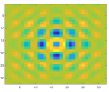
(a) True Kernel $A^{\ast}$

(b) Observations $Y$

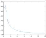
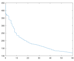
(c) Objective value over time (s). The left plot shows ADMM-slack, and the right shows ADMM-exact.

(d) Kernel matrices $A$ for ADMM-slack at iterations $k=0,10,20,50,100$.

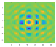
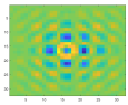
(e) Kernel matrices $A$ for ADMM-exact at iterations $k=0,10,50,100,150$.

Figure 2. ADMM-slack and ADMM-exact, noiseless.

We first compare ADMM-exact and ADMM-slack on noiseless data to assess the impact of the slack variable in (SBD1), which makes the formulation inexact. Figures 2, 3 and 4 show the performance of ADMM-exact and ADMM-slack on synthetic problems generated according to (E.1) with $\xi=0$. The top row of each figure shows the true kernel, the observation data $Y$, and the objective values over 60 seconds for ADMM-slack and ADMM-exact. To measure both the sparsity and accuracy, the objective function reported is given by $\frac{1}{10}\|X\|_{1}+\frac{1}{2}\|Y-A\ast X-b\mathbf{1}\|_{F}^{2}$. The next two rows shows the kernel matrix $A$ recovered by each method at various stages of progress. In the noiseless case, the performance of ADMM-exact and ADMM-slack appears to be similar. We also observe empirically that the convergence is sublinear, which is consistent with the general rate $O(\frac{1}{k})$ for ADMM.

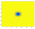
(a) True Kernel $A^{\ast}$

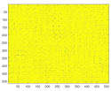
(b) Observations $Y$

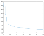
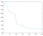
(c) Objective value over time (s). The left plot shows ADMM-slack, and the right shows ADMM-exact.

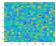
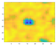
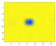
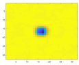
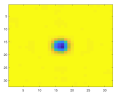
(d) Kernel matrices $A$ for ADMM-slack at iterations $k=0,10,20,30,50$.

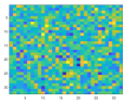
(e) Kernel matrices $A$ for ADMM-exact at iterations $k=0,10,50,100,120$.

Figure 3. ADMM-slack and ADMM-exact, noiseless.

(a) True Kernel $A^{\ast}$

(b) Observations $Y$

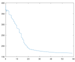
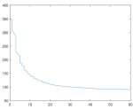
(c) Objective value over time (s). The left plot shows ADMM-slack, and the right shows ADMM-exact.

(d) Kernel matrices $A$ for ADMM-slack at iterations $k=0,10,30,50,100$.

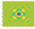
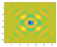
(e) Kernel matrices $A$ for ADMM-exact at iterations $k=0,10,20,50,100$.

Figure 4. ADMM-slack and ADMM-exact, noiseless.

E.1. Noisy Observations

We next consider the case where the observations $Y$ are corrupted by noise. In this case, the formulation (SBD1) is more natural because $A\ast X+b\mathbf{1}=Y$ cannot be satisfied exactly, even by the true $A,X,b$. The slack variable $Z$ then serves to absorb the noise term $\xi$.

(a) True Kernel $A^{\ast}$

(b) Observations $Y$ (with noise)

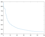
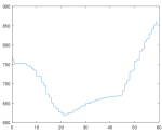
(c) Objective value over time (s). The left plot shows ADMM-slack, and the right shows ADMM-exact.

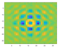
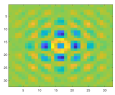
(d) Kernel matrices $A$ for ADMM-slack at iterations $k=0,10,20,50,100$.

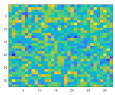
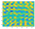
(e) Kernel matrices $A$ for ADMM-exact at iterations $k=0,10,50,100,200$.

Figure 5. ADMM-slack and ADMM-exact on noisy observations.

We observe in Figure 5 that while ADMM-slack converges even in the presence of noise, ADMM-exact eventually begins to diverge. Since the constraint cannot be satisfied exactly, the Lagrange multipliers grow over time, causing $A,X$ to behave erratically to overfit to the noise and decreasing the relative importance of the sparsity of $X$. This suggests that for practical applications, where a certain amount of noise is unavoidable, the formulation (SBD1) with the slack variable $Z$ is both more practical, as well as being provably convergent within our framework.

Figures 6 and 7 show additional examples in the noisy setting.

(a) True Kernel $A^{\ast}$

(b) Observations $Y$ (with noise)

(c) Objective value over time (s). The left plot shows ADMM-slack, and the right shows ADMM-exact.

(d) Kernel matrices $A$ for ADMM-slack at iterations $k=0,10,20,50,100$.

(e) Kernel matrices $A$ for ADMM-exact at iterations $k=0,10,20,100,200$.

Figure 6. ADMM-slack and ADMM-exact on noisy observations.

(a) True Kernel $A^{\ast}$

(b) Observations $Y$ (with noise)

(c) Objective value over time (s). The left plot shows ADMM-slack, and the right shows ADMM-exact.

(d) Kernel matrices $A$ for ADMM-slack at iterations $k=0,10,50,100,150$.

(e) Kernel matrices $A$ for ADMM-exact at iterations $k=0,10,50,100,200$.

Figure 7. ADMM-slack and ADMM-exact on noisy observations.

References

- [1] H. Attouch, J. Bolte, P. Redont, and A. Soubeyran, Proximal alternating minimization and projection methods for nonconvex problems: An approach based on the kurdyka-łojasiewicz inequality, Mathematics of Operations Research, 35 (2010), pp. 438–457.
- [2] H. Attouch, J. Bolte, and B. F. Svaiter, Convergence of descent methods for semi-algebraic and tame problems: proximal algorithms, forward–backward splitting, and regularized gauss–seidel methods, Mathematical Programming, 137 (2013), pp. 91–129.
- [3] X. Bai and K. Scheinberg, Alternating direction methods for non convex optimization with applications to second-order least-squares and risk parity portfolio selection, tech. rep., 2015. http://www.optimization-online.org/DB_HTML/2015/02/4776.html.
- [4] J. Bolte, S. Sabach, and M. Teboulle, Nonconvex lagrangian-based optimization: Monitoring schemes and global convergence, Mathematics of Operations Research, 43 (2018), pp. 1210–1232.
- [5] R. I. Bo\textcommabelowt and D.-K. Nguyen, The proximal alternating direction method of multipliers in the non-convex setting: convergence analysis and rates, arXiv:1801.01994, (2018).
- [6] S. Boyd, N. Parikh, E. Chu, B. Peleato, and J. Eckstein, Distributed optimization and statistical learning via the alternating direction method of multipliers, Foundations and Trends in Machine Learning, 3 (2011), pp. 1–122.
- [7] S. Burer and R. D. C. Monteiro, A nonlinear programming algorithm for solving semidefinite programs via low-rank factorization, Mathematical Programming, 95 (2003), pp. 329–357.
- [8] E. J. Candès, X. Li, Y. Ma, and J. Wright, Robust principal component analysis?, Journal of the ACM, 58 (2011).
- [9] C. Chen, B. He, Y. Ye, and X. Yuan, The direct extension of ADMM for multi-block convex minimization problems is not necessarily convergent, Mathematical Programming, 155 (2016), pp. 57–79.
- [10] L. Chen, D. Sun, and K.-C. Toh, An efficient inexact symmetric gauss–seidel based majorized ADMM for high-dimensional convex composite conic programming, Mathematical Programming, 161 (2017), pp. 237–270.
- [11] , A note on the convergence of ADMM for linearly constrained convex optimization problems, Computational Optimization and Applications, 66 (2017), pp. 327–343.
- [12] Y. Cui, X. Li, D. Sun, and K.-C. Toh, On the convergence properties of a majorized alternating direction method of multipliers for linearly constrained convex optimization problems with coupled objective functions, Journal of Optimization THeory and Applications, 169 (2016), pp. 1013–1041.
- [13] D. Davis and W. Yin, A three-operator splitting scheme and its optimization applications, Set-Valued and Variational Analysis, 25 (2017), pp. 829–858.
- [14] W. Deng, M.-J. Lai, Z. Peng, and W. Yin, Parallel multi-block ADMM with o(1/k) convergence, Journal of Scientific Computing, 71 (2017), pp. 712–736.
- [15] D. Driggs, S. Becker, and A. Aravkin, Adapting regularized low-rank models for parallel architectures, (2017). https://arxiv.org/abs/1702.02241.
- [16] J. Eckstein and D. Bertsekas, On the douglas-rachford splitting method and the proximal point algorithm for maximal monotone operators, Mathematical Programming, 55 (1992), pp. 293–318.
- [17] J. Eckstein and W. Yao, Understanding the convergence of the alternating direction method of multipliers: Theoretical and computational perspectives, Pacific Journal on Optimization, 11 (2015), pp. 619–644.
- [18] M. Elad and M. Aharon, Image denoising via sparse and redundant representations over learned dictionaries, IEEE Transactions on Image Processing, 15 (2006), pp. 3736–3745.
- [19] M. Fazel, T. K. Pong, D. Sun, and P. Tseng, Hankel matrix rank minimization with applications to system identification and realization, SIAM Journal on Matrix Analysis and Applications, 34 (2013), pp. 946–977.
- [20] D. Gabay and B. Mercier, A dual algorithm for the solution of nonlinear variational problems via finite element approximation, Computers & Mathematics with Applications, 2 (1976), pp. 17–40.
- [21] R. Glowinski and A. Marroco, On the approximation by finite elements of order one, and resolution, penalisation-duality for class of nonlinear dirichlet problems, ESAIM: Mathematical Modelling and Numerical Analysis, 9 (1975), pp. 41–76.
- [22] M. X. Goemans and D. P. Williamson, Improved approximation algorithms for maximum cut and satisfiability problems using semidefinite programming, Journal of the ACM, 42 (1995), pp. 1115–1145.
- [23] D. Hajinezhad, T.-H. Chang, X. Wan, Q. Shi, and M. Hong, Nonnegative matrix factorization using ADMM: Algorithm and convergence analysis, 2016 IEEE International Conference on Acoustics, Speech and Signal Processing (ICASSP), (2016), pp. 4742–4746.
- [24] D. Han and X. Yuan, A note on the alternating direction method of multipliers, Journal of Optimization Theory and Applications, 155 (2012), pp. 227–238.
- [25] M. Hong, Z.-Q. Luo, and M. Razaviyayn, Convergence analysis of alternating direction method of multipliers for a family of nonconvex problems, SIAM Journal on Optimization, 26 (2016), pp. 337–364.
- [26] M. Hubert and S. Engelen, Robust pca and classification in biosciences, Bioinformatics, 20 (2004), pp. 1728–1736.
- [27] R. Janin, Directional derivative of the marginal function in nonlinear programming, in Sensitivity, Stability, and Parametric Analysis, Mathematical Programming Studies, A. V. Fiacco, ed., vol. 2, Springer, Berlin, Heidelberg, 1984.
- [28] B. Jiang, T. Lin, S. Ma, and S. Zhang, Structured nonconvex and nonsmooth optimization: Algorithms and iteration complexity analysis, Computational Optimization and Applications, 72 (2019), pp. 115–157.
- [29] B. Jiang, S. Ma, and S. Zhang, Alternating direction method of multipliers for real and complex polynomial optimization models, Optimization, 63 (2014), pp. 883–898.
- [30] R. M. Karp, Reducibility among combinatorial problems, in Complexity of Computer Computations, IBM Research Symposia Series, R. E. Miller, J. W. Thatcher, and J. D. Bohlinger, eds., Springer, 1972, pp. 85–103.
- [31] D. D. Lee and H. S. Seung, Learning the parts of objects by non-negative matrix factorization, Nature, 401 (1999), pp. 788–791.
- [32] , Algorithms for non-negative matrix factorization, Advances in Neural Information Processing Systems, 13 (2000).
- [33] G. Li and T. K. Pong, Global convergence of splitting methods for nonconvex composite optimization, SIAM Journal on Optimization, 25 (2015), pp. 2434–2460.
- [34] M. Li, D. Sun, and K.-C. Toh, A convergent 3-block semi-proximal ADMM for convex minimization problems with one strongly convex block, Asia-Pacific Journal of Operational Research, 32 (2015), p. 1550024.
- [35] , A majorized ADMM with indefinite proximal terms for linearly constrained convex composite optimization, SIAM Journal on Optimization, 26 (2016), pp. 922–950.
- [36] X. Li, D. Sun, and K.-C. Toh, A schur complement based semi-proximal ADMM for convex quadratic conic programming and extensions, Mathematical Programming, 155 (2016), pp. 333–373.
- [37] T. Lin, S. Ma, and S. Zhang, On the global linear convergence of the ADMM with multi-block variables, SIAM Journal on Optimization, 26 (2015), pp. 1478–1497.
- [38] , On the sublinear convergence rate of multi-block ADMM, Journal of the Operations Research Society of China, 3 (2015), pp. 251–271.
- [39] , Global convergence of unmodified 3-block ADMM for a class of convex minimization problems, Journal of Scientific Computing, 76 (2018), pp. 69–88.
- [40] Z. Lin, R. Liu, and H. Li, Linearized alternating direction method with parallel splitting and adaptive penalty for separable convex programs in machine learning, Machine Learning, 99 (2015), pp. 287–325.
- [41] P.-L. Lions and B. Mercier, Splitting algorithms for the sum of two nonlinear operators, SIAM Journal on Numerical Analysis, 16 (1979), pp. 964–979.
- [42] S. Lu, Implications of the constant rank constraint qualification, Mathematical Programming, 126 (2011), pp. 365–392.
- [43] J. Mairal, F. Bach, J. Ponce, and G. Sapiro, Online learning for matrix factorization and sparse coding, Journal of Machine Learning Research, 11 (2010), pp. 19–60.
- [44] Yu. Nesterov, Smooth minimization of non-smooth functions, Mathematical Programming, 103 (2005), pp. 127–152.
- [45] R. T. Rockafellar and R. J.-B. Wets, Variational Analysis, Grundlehren der mathematischen Wissenschaften 317, Springer-Verlag Berlin Heidelberg, 1st ed., 1997.
- [46] E. Ryu, Uniqueness of DRS as the 2 operator resolvent-splitting and impossibility of 3 operator resolvent-splitting, (2018). https://arxiv.org/abs/1802.07534.
- [47] W. Shi, Q. Ling, K. Yuan, G. Wu, and W. Yin, On the linear convergence of the ADMM in decentralized consensus optimization, IEEE Transactions on Signal Processing, 62 (2014), pp. 1750–1761.
- [48] A. Sokal, A really simple elementary proof of the uniform boundedness theorem, American Mathematical Monthly, 118 (2011), pp. 450–452.
- [49] D. Sun, K. Toh, and L. Yang, A convergent 3-block semiproximal alternating direction method of multipliers for conic programming with 4-type constraints, SIAM Journal on Optimization, 25 (2015), pp. 882–915.
- [50] J. Sun, Q. Qu, and J. Wright, Complete dictionary recovery over the sphere i: Overview and the geometric picture, IEEE Trans. Information Theory, 63 (2017), pp. 853–884.
- [51] , Complete dictionary recovery over the sphere ii: Recovery by riemannian trust-region method, IEEE Trans. Information Theory, 63 (2017), pp. 885–914.
- [52] M. Sun and H. Sun, Improved proximal ADMM with partially parallelsplitting for multi-block separable convex programming, Journal of Applied Mathematics and Computing, 58 (2018), pp. 151–181.
- [53] G. Taylor, R. Burmeister, Z. Xu, B. Singh, A. Patel, and T. Goldstein, Training neural networks without gradients: A scalable ADMM approach, Proceedings of the 33rd International Conference on Machine Learning (PMLR), 48 (2016), pp. 2722–2731.
- [54] R. Tibshirani, Regression shrinkage and selection via the lasso, Journal of the Royal Statistical Society, Series B, 58 (1996), pp. 267–288.
- [55] J. J. Wang and W. Song, An algorithm twisted from generalized ADMM for multi-block separable convex minimization models, Journal of Computational and Applied Mathematics, 309 (2017), pp. 342–358.
- [56] S. Wang, L. Zhang, Y. Liang, and Q. Pan, Semi-coupled dictionary learning with applications to image super-resolution and photo-sketch synthesis, Computer Vision and Pattern Recognition, (2012).
- [57] Y. Wang, W. Yin, and J. Zeng, Global convergence of ADMM in nonconvex nonsmooth optimization, Journal of Scientific Computing, 78 (2019), pp. 29–63.
- [58] Y. Xu, W. Yin, Z. Wen, and Y. Zhang, An alternating direction algorithm for matrix completion with nonnegative factors, Frontiers of Mathematics in China, 7 (2012), pp. 365–384.
- [59] Yurii Nesterov and B. Polyak, Cubic regularization of newton method and its global performance, Mathematical Programming, 108 (2006), pp. 177–205.
- [60] J. Zhang, S. Ma, and S. Zhang, Primal-dual optimization algorithms over riemannian manifolds: an iteration complexity analysis, (2017). https://arxiv.org/abs/1710.02236.