Revisiting Totally Positive Differential Systems: A Tutorial and New Results

Abstract

A matrix is called totally nonnegative (TN) [totally positive (TP)] if all its minors are nonnegative [positive]. Multiplying a vector by a TN matrix does not increase the number of sign variations in the vector. In a largely forgotten paper, Binyamin Schwarz (1970) considered matrices whose exponentials are TN or TP. He also analyzed the evolution of the number of sign changes in the vector solutions of the corresponding linear system. His work, however, considered only linear systems.

In a seemingly different line of research, Smillie (1984), Smith (1991), and others analyzed the stability of nonlinear tridiagonal cooperative systems by using the number of sign variations in the derivative vector as an integer-valued Lyapunov function.

We show that these two research topics are intimately related. This allows to derive important generalizations of the results by Smillie (1984) and Smith (1991) while simplifying the proofs. These generalizations are particularly relevant in the context of control systems. Also, the results by Smillie and Smith provide sufficient conditions for analyzing stability based on the number of sign changes in the vector of derivatives and the connection to the work of Schwarz allows to show in what sense these results are also necessary. We describe several new and interesting research directions arising from this new connection.

Keywords: Totally nonnegative matrices, totally positive matrices, infinitesimal generators, cooperative dynamical systems, monotone dynamical systems, entrainment, Floquet theory, stability analysis, multiplicative and additive compound matrices.

1 Introduction

The trajectories of monotone dynamical systems preserve a partial ordering, induced by a proper cone, between their initial conditions. Hirsch’s quasi-convergence theorem (Smith, 1995) shows that this property has far reaching implications for the asymptotic behavior of their trajectories. An important special case are cooperative systems arising when the cone that induces the partial ordering is the positive orthant. In an interesting paper, Smillie (1984) considered the time-invariant, nonlinear, strongly cooperative, and tridiagonal system:

$$\dot{x}(t)=f(x(t)),$$ (1)

where $x(t)\in\mathbb{R}^{n}$ and $f:\mathbb{R}^{n}\to\mathbb{R}^{n}$, and has shown that every trajectory either leaves any compact set or converges to an equilibrium point. This result has found many applications as well as several interesting generalizations (see, e.g. Margaliot and Tuller (2012); Chua and Roska (1990); Donnell et al. (2009); Smith (1991); Fang et al. (2013)).

To explain Smillie’s proof, let $z:=\dot{x}$. Then (1) yields the variational equation

$$\dot{z}(t)=J(x(t))z(t),$$ (2)

where $J(x):=\frac{\partial}{\partial x}f(x)$ is the Jacobian of the vector field $f$. Smillie showed that since $J$ is tridiagonal with positive entries on the super- and sub-diagonal, the number of sign variations in the vector $z(t)$, denoted $\sigma(z(t))$, is a non-increasing function of $t$. Recall that for a vector $y\in\mathbb{R}^{n}$ with no zero entries the number of sign variations in $y$ is

$$\sigma(y):=\left|\{i\in\{1,\dots,n-1\}:y_{i}y_{i+1}<0\}\right|.$$ (3)

For example, for $n=3$ consider the vector $z(\varepsilon):=\begin{bmatrix}-1&\varepsilon&2\end{bmatrix}^{\prime}$. For any $\varepsilon\in\mathbb{R}\setminus\{0\}$, $\sigma(z(\varepsilon))$ is well-defined and equal to one. More generally, the function $\sigma$ can be extended, via continuity, to the largest open set:

$$\mathcal{V}:= \{y\in\mathbb{R}^{n}:y_{1}\not=0,\;y_{n}\not=0,\;\text{and if }y_{i}=0$$

$$\text{ for some~{}$i\in\{2,\dots,n-1\}$ then }y_{i-1}y_{i+1}<0\}.$$

Note in particular that if $y\in\mathcal{V}$ then $y$ cannot have two adjacent zero coordinates.

To explain the basic idea underlying Smillie’s proof, consider the case $n=3$. Seeking a contradiction, assume that the sign pattern of $z(t)$ near some time $t=t_{0}$ is as follows:

	$t=t_{0}^{-}$	$t=t_{0}$	$t=t_{0}^{+}$
$z_{1}(t)$	$+$	$+$	$+$
$z_{2}(t)$	$+$	$0$	$-$
$z_{3}(t)$	$+$	$+$	$+$

Note that in this case $\sigma(t):=\sigma(z(t))$ increases from $\sigma(t_{0}^{-})=0$ to $\sigma(t_{0}^{+})=2$. However, using (2) and the structure of $J$ yields $\dot{z}(t_{0})=\begin{bmatrix}*&+&0\\ +&*&+\\ 0&+&*\end{bmatrix}\begin{bmatrix}+\\ 0\\ +\end{bmatrix},$ where $+$ means a positive value, and $*$ means some value, and thus $\dot{z}_{2}(t_{0})>0$, and the case described in the table above cannot take place. Smillie’s analysis shows rigorously that when $\sigma(t)$ changes it can only decrease. This is based on direct analysis of the ODEs and is non trivial due to the fact that if an entry $z_{i}(t)$ becomes zero at some time $t=t_{0}$ (thus perhaps leading to a change in $\sigma(t)$ near $t_{0}$) one must consider the possibility that higher-order derivatives of $z_{i}(t)$ are also zero at $t=t_{0}$. Smillie then used the behavior of $\sigma(z(t))$ to deduce that for any point $a$ in the state-space of (1) the omega limit set $\omega(a)$ cannot include more than a single point, and thus every trajectory either leaves any compact set or converges to an equilibrium point.

Smith (1991) extended Smillie’s approach to the case of a time-varying cooperative system with a tridiagonal Jacobian with positive entries on the super- and sub-diagonals for all time $t$. He showed that if the time-varying vector field is periodic with period $T$ then every solution of the nonlinear dynamical system either leaves any compact set or converges to a periodic solution with period $T$. Fang et al. (2013) describe some generalizations of these ideas to time-recurrent systems. The main advantage of this analysis approach is that it allows to study the global behavior of the nonlinear system (1) using the (time-varying) linear system (2).

Here, we show that these results can be generalized, and their proofs simplified, by relating them to a classical topic from linear algebra: the sign variation diminishing property (SVDP) of totally nonnegative (TN) matrices (Fallat and Johnson, 2011; Pinkus, 2010), and more precisely to the notion of totally positive differential systems (TPDSs) introduced by Schwarz (1970).

To explain this, we recall two more definitions for the number of sign variations in a vector (Fallat and Johnson, 2011). For $y\in\mathbb{R}^{n}$, let $s^{-}(y)$ denote the number of sign variations in the vector $y$ after deleting all its zero entries, and let $s^{+}(y)$ denote the maximal possible number of sign variations in $y$ after each zero entry is replaced by either $+1$ or $-1$. Note that $s^{-}(y)\leq s^{+}(y)$ for all $y\in\mathbb{R}^{n}$. For example, for $y=\begin{bmatrix}1&0&2&-3&0&1.1\end{bmatrix}^{\prime}$, $s^{-}(y)=2$ and $s^{+}(y)=4$. Let $\mathcal{W}:=\{y\in\mathbb{R}^{n}:s^{-}(y)=s^{+}(y)\}.$ Note that if $y\in\mathcal{W}$ then $y$ cannot have two adjacent zero coordinates. An immediate yet important observation is that $\mathcal{W}=\mathcal{V}$. Thus, if $y\in\mathcal{W}$ then $s^{-}(y)=s^{+}(y)=\sigma(y)$.

A classical result from the theory of TN matrices (Fallat and Johnson, 2011) states that if $A\in\mathbb{R}^{n\times m}$ is totally positive (TP) and $x\in\mathbb{R}^{m}\setminus\{0\}$ then $s^{+}(Ax)\leq s^{-}(x)$, whereas if $A$ is TN (and in particular if it is TP) then $s^{-}(Ax)\leq s^{-}(x)$ for all $x\in\mathbb{R}^{m}$. To apply this SVDP to the stability analysis of (1) note that if the transition matrix corresponding to $J(x(t))$ in (2) is TP for all time $t$ then we may expect the number of sign variations in $z(t)$ to be a nonincreasing function of time. As already shown by Smillie (1984), this implies that there exists a time $s\geq 0$ such that $x_{1}(t)$ and $x_{n}(t)$ are monotone functions of time for all $t\geq s$, and that every trajectory of (1) either leaves any compact set or converges to an equilibrium point.

Schwarz (1970) considered the linear matrix differential equation $\dot{Y}(t)=A(t)Y(t)$, $Y(t_{0})=I$, with $A(t)\in\mathbb{R}^{n\times n}$ a continuous matrix function of $t$. Note that every minor of $I$ is nonnegative (as it is either zero or one). Schwarz gave a formula for the induced dynamics of the minors of $Y(t)$. He defined the system as a totally [nonnegative] positive dynamical system if for every $t_{0}$ and every $t>t_{0}$ the matrix $Y(t)$ is TP [TN]. His analysis is based on what is now known as the theory of cooperative dynamical systems: the system is a totally nonnegative dynamical system if the dynamics maps any set of nonnegative minors to a set of nonnegative minors. However, the work of Schwarz seems to have been largely forgotten and its potential for the analysis of nonlinear dynamical systems has been overlooked. Indeed, according to Google Scholar Schwarz’s paper has been cited $22$ times since its publication in $1970$.

We show that TPDSs can be immediately linked to recent results on the stability of nonlinear cooperative systems. We consider a more general form than in Schwarz (1970), namely, $\dot{Y}(t)=A(t)Y(t)$, with $A(t)$ a measurable matrix function of time rather than continuous.

We then show how this can be used to derive the interesting results of Smillie (1984) and Smith (1991) under milder technical conditions and with simpler proofs. These generalizations are particularly relevant to control systems.

The next section reviews relevant definitions and results from the theory of TN matrices. Section 3 reviews TPDSs. Section 4 shows how these results can be applied to analyze the stability of nonlinear time-varying tridiagonal cooperative systems. We believe that highlighting the deep connections between the work of Schwarz and more recent work on nonlinear tridiagonal cooperative systems opens the door for many new research directions. Some of these potential directions are described in Section 5. The work of Schwarz has been largely forgotten, and TN matrices are not well-known in the systems and control community, so we provide a self-contained tutorial on the tools needed for the stability analysis of nonlinear systems.

We use standard notation. Vectors [matrices] are denoted by small [capital] letters. $\mathbb{R}^{n}$ is the set of vectors with $n$ real coordinates. For a (column) vector $x\in\mathbb{R}^{n}$, $x_{i}$ is the $i$th entry of $x$, and $x^{\prime}$ is the transpose of $x$. Let $\mathbb{R}^{n}_{++}:=\{v\in\mathbb{R}^{n}:v_{i}>0,i=1,\dots,n\}$, i.e. the set of all $n$-dimensional vectors with positive entries. A square matrix $B$ is called Metzler if every off-diagonal entry of $B$ is nonnegative. The square identity matrix is denoted by $I$, with dimension that should be clear from context.

2 TN and TP matrices

We begin by reviewing known definitions and results from the rich and beautiful theory of TN and TP matrices that will be used later on. We consider only square and real matrices, as this is the case that is relevant for our applications. For more information and proofs we refer to the two excellent monographs (Fallat and Johnson, 2011; Pinkus, 2010). Unfortunately, this field suffers from nonuniform terminology. We follow the more modern terminology in (Fallat and Johnson, 2011).

Definition 1.

A matrix $A\in\mathbb{R}^{n\times n}$ is called totally nonnegative [totally positive] if the determinant of every square submatrix is nonnegative [positive].

In particular, if $A$ is TN [TP] then every entry of $A$ is nonnegative [positive].

Example 1.

It is straightforward to verify that the matrix $A=\begin{bmatrix}0&1&0\\ 0&0&1\\ 0&0&0\end{bmatrix}$ is TN. Consider the permutation matrix $P:=\begin{bmatrix}0&1&0\\ 0&0&1\\ 1&0&0\end{bmatrix}$. Then $PAP^{-1}=\begin{bmatrix}0&1&0\\ 0&0&0\\ 1&0&0\end{bmatrix}$ is not TN because $\det\left(\begin{bmatrix}0&1\\ 1&0\end{bmatrix}\right)<0$.

Determining that an $n\times n$ matrix is TN [TP] by direct verification of Def. 1 requires checking the signs of all its $\sum_{k=1}^{n}\binom{n}{k}^{2}$ minors. This is of course prohibitive. Fortunately, the minors are not independent and thus there exist much more efficient methods for verifying that a matrix is TN [TP] (Fallat and Johnson, 2011, Ch. 3). Also, some matrices with a special structure are known to be TN. We review two such examples. The first is important in proving the SVDP of TN matrices. The second example, as we will see below, is closely related to Smillie’s results.

Example 2.

Let $E_{i,j}$ denote the $n\times n$ matrix with all entries zero, except for entry $(i,j)$ that is one. For $p\in\mathbb{R}$ and $i\in\{2,\dots,n\}$, let

$$L_{i}(p):=I+pE_{i,i-1},\;\;U_{i}(p):=I+pE_{i-1,i}.$$ (4)

Matrices in this form are called elementary bidiagonal (EB) matrices. If the identity matrix $I$ in (4) is replaced by a diagonal matrix $D$ then the matrices are called generalized elementary bidiagonal (GEB). It is straightforward to see that EB matrices are TN when $p\geq 0$, and that GEB matrices are TN when $p\geq 0$ and the diagonal matrix $D$ is componentwise nonnegative.

Example 3.

Consider the tridiagonal matrix

$$A=\begin{bmatrix}a_{1}&b_{1}&0&\dots&0\\ c_{1}&a_{2}&\ddots&\dots&\vdots\\ 0&\ddots&\ddots&\dots&\vdots\\ \vdots&\ddots&\ddots&\dots&b_{n-1}\\ 0&\dots&\dots&c_{n-1}&a_{n}\end{bmatrix}$$ (5)

with $b_{i},c_{i}\geq 0$ for all $i$. In this case, the dominance condition

$$a_{i}\geq b_{i}+c_{i-1}\quad\text{for all }i\in\{1,\dots,n\},$$ (6)

with $c_{0}:=0$ and $b_{n}:=0$, guarantees that $A$ is TN (Fallat and Johnson, 2011, Ch. 0).

An important subclass of TN matrices are the oscillatory matrices studied in the pioneering work of Gantmacher and Krein (2002). A matrix $A\in\mathbb{R}^{n\times n}$ is called oscillatory if $A$ is TN and there exists an integer $k>0$ such that $A^{k}$ is TP. It is well-known that a TN matrix $A$ is oscillatory if and only if it is non-singular and irreducible (Fallat and Johnson, 2011, Ch. 2), and that in this case $A^{n-1}$ is TP.

Example 4.

Consider the matrix $A=\begin{bmatrix}2&1&0\\ 1&2&1\\ 0&1&2\end{bmatrix}.$ This matrix is TN, non-singular and irreducible, so it is an oscillatory matrix. Here $A^{n-1}=A^{2}=\begin{bmatrix}5&4&1\\ 4&6&4\\ 1&4&5\end{bmatrix},$ and it is straightforward to verify that this matrix is indeed TP.

More generally, the matrix $A$ in (5) satisfying $b_{i},c_{i}>0$, $i=1,\dots,n-1$, and the dominance condition (6) is TN and irreducible. If it is also non-singular then it is oscillatory.

An important property, that will be used throughout, is that the product of two TN [TP] matrices is a TN [TP] matrix. This follows immediately from Def. 1 and the Cauchy-Binet formula for the minors of the product of two matrices (Horn and Johnson, 2013, Ch. 0). (A straightforward proof of several important determinantal identities can be found in Brualdi and Schneider (1983).)

When using TN matrices to study dynamical systems, it is important to bear in mind that in general coordinate transformations do not preserve TN (see Example 1 above). An important exception, however, is positive diagonal scaling. Indeed, if $D$ is a diagonal matrix with positive entries on the diagonal then multiplying a matrix $A$ by $D$ either on the left or right changes the sign of no minor, so in particular $DAD^{-1}$ is TN [TP] if and only if $A$ is TN [TP].

At this point we can already provide an intuitive explanation revealing the so far unknown connection between Smillie’s results and TN matrices. To do this, consider for simplicity the system $\dot{z}=Jz$, with $J$ a constant tridiagonal matrix with positive entries on the super- and sub-diagonals. Then to first order in $t$ we have $z(t)=(I+tJ)z(0)$, and for any sufficiently small $t>0$ the matrix $I+tJ$ is TN (see Example 3), irreducible, and non-singular, so it is an oscillatory matrix.

2.1 Spectral properties of TN matrices

TN matrices have a strong spectral structure: all their eigenvalues are real and nonnegative, and the corresponding eigenvectors have special sign patterns. This spectral structure is particularly evident in the case of oscillatory matrices.

Theorem 1.

(Pinkus, 1996) If $A\in\mathbb{R}^{n\times n}$ is an oscillatory matrix then its eigenvalues are all real, positive, and distinct. If we order the eigenvalues as $\lambda_{1}>\lambda_{2}>\dots>\lambda_{n}>0$ and let $u^{k}\in\mathbb{R}^{n}$ denote the eigenvector corresponding to $\lambda_{k}$ then for any $1\leq i\leq j\leq n$ and any scalars $c_{i},\dots,c_{j}$ that are not all zero

$$i-1\leq s^{-}(\sum_{k=i}^{j}c_{k}u^{k})\leq s^{+}(\sum_{k=i}^{j}c_{k}u^{k})\leq j-1.$$

In particular,

$$s^{-}(u^{i})=s^{+}(u^{i})=i-1,\quad i=1,\dots,n.$$ (7)

Note that eigenvectors may have some zero coordinates, but (7) implies that $u^{i}\in\mathcal{V}$ for all $i$.

Example 5.

Consider the TP matrix $A=\begin{bmatrix}5&4&1\\ 4&6&4\\ 1&4&5\end{bmatrix}$. Its eigenvalues are $\lambda_{1}=2(3+2\sqrt{2})$, $\lambda_{2}=4$, $\lambda_{3}=2(3-2\sqrt{2})$ with corresponding eigenvectors $u^{1}=\begin{bmatrix}1&\sqrt{2}&1\end{bmatrix}^{\prime}$, $u^{2}=\begin{bmatrix}-1&0&1\end{bmatrix}^{\prime}$, and $u^{3}=\begin{bmatrix}1&-\sqrt{2}&1\end{bmatrix}^{\prime}$. Note that $s^{-}(u^{k})=s^{+}(u^{k})=k-1$ for $k=1,2,3$.

Note that $A$ oscillatory implies that $A$ is componentwise nonnegative and that $A^{\ell}$ is TP for some integer $\ell\geq 1$ and thus by the Perron-Frobenius Thm. (Horn and Johnson, 2013) $A^{\ell}$ (and thus $A$) has a real positive eigenvalue $\lambda_{1}$ with maximum modulus and the corresponding eigenvector $u^{1}$ has positive entries, i.e. $s^{-}(u^{1})=s^{+}(u^{1})=0$. Thm. 1 shows that for oscillatory matrices a much stronger spectral structure arises.

2.2 Sign variation diminishing property of TN matrices

TN matrices enjoy a remarkable variety of mathematical properties. For our purposes, the most relevant property is that multiplication by a TN matrix cannot increase the sign variation of a vector. This is the sign variation diminishing property (SVDP) of linear TN transformations.

Let $A$ be a TN EB matrix. Pick $x\in\mathbb{R}^{n}$, and let $y:=Ax$. Then there exists at most one index $i$ such that $\operatorname{{\mathrm{s}gn}}(y_{i})\not=\operatorname{{\mathrm{s}gn}}(x_{i})$, and either $y_{i}=x_{i}+px_{i-1}$ or $y_{i}=x_{i}+px_{i+1}$, and since $p\geq 0$ the sign can change only in the “direction” of $x_{i-1}$ or $x_{i+1}$. In either case, neither $s^{-}$ or $s^{+}$ may increase. We conclude that if $A$ is TN EB then

$$s^{-}(Ax) \leq s^{-}(x)\text{ for all }x\in\mathbb{R}^{n},$$ (8)

and

$$s^{+}(Ax) \leq s^{+}(x)\text{ for all }x\in\mathbb{R}^{n}.$$ (9)

A similar argument shows that if $A$ is TN GEB then (8) holds. However, (9) does not hold in general for a TN GEB matrix $A$. For example, $A=0$ is TN GEB and clearly $s^{+}(Ax)=s^{+}(0)=n-1$ may be larger than $s^{+}(x)$.

This SVDP can be extended to all TN matrices using the following fundamental decomposition result.

Theorem 2.

(Fallat and Johnson, 2011, Ch. 2) Any TN matrix can be expressed as a product of TN GEB matrices.

Example 6.

For the simplest example of this bidiagonal factorization, consider the case $n=2$. Suppose that $A=\begin{bmatrix}a_{11}&a_{12}\\ a_{21}&a_{22}\end{bmatrix}$ is TN, that is, $a_{ij}\geq 0$, $i,j=1,2$, and $\det(A)=a_{11}a_{22}-a_{12}a_{21}\geq 0$. We consider two cases. If $a_{11}>0$ then $A=\begin{bmatrix}1&0\\ a_{21}/a_{11}&1\end{bmatrix}\begin{bmatrix}a_{11}&0\\ 0&\det(A)/a_{11}\end{bmatrix}\begin{bmatrix}1&a_{12}/a_{11}\\ 0&1\end{bmatrix},$ and this is a product of the required form. If $a_{11}=0$ then the TN of $A$ implies that $a_{12}a_{21}=0$. Assume without loss of generality that $a_{12}=0$. Then $A=\begin{bmatrix}0&0\\ a_{21}&1\end{bmatrix}\begin{bmatrix}1&0\\ 0&a_{22}\end{bmatrix},$ and this is again a product of the required form.

Combining Thm. 2 with the fact that (8) holds for all TN GEB matrices implies that (8) holds for any TN matrix $A$.

Remark 1.

As noted above, $A$ TN does not imply (9). However, (9) does hold if $A$ is a nonsingular TN matrix (Fallat and Johnson, 2011, Ch. 4).

TP matrices satisfy a stronger SVDP.

Theorem 3.

(Fallat and Johnson, 2011, Ch. 4) If $A\in\mathbb{R}^{n\times n}$ is TP then

$$s^{+}(Ax)\leq s^{-}(x)\text{ for all }x\in\mathbb{R}^{n}\setminus\{0\}.$$ (10)

If $A$ is TN and nonsingular then $s^{+}(Ax)\leq s^{-}(x)$ for all $x\in\mathbb{R}^{n}$ such that either $x$ has no zero entries or $Ax$ has no zero entries.

A natural question is whether SVDP characterizes TN or TP matrices. Recall that a matrix is called strictly sign-regular (SSR) if for every $k$ all minors of order $k$ are non-zero and share a common sign (that may vary from size to size). For example, $A=\begin{bmatrix}1&2\\ 3&1\end{bmatrix}$ is SSR because all minors of order one are positive, and the single minor of order two is non-zero. Obviously, TP matrices are SSR.

Theorem 4.

Let $A\in\mathbb{R}^{n\times n}$ be a nonsingular matrix. Then the following properties are equivalent.

1. $A$ is SSR.

2. $s^{+}(Ax)\leq s^{-}(x)$ for all $x\in\mathbb{R}^{n}\setminus\{0\}$.

Note that the first assertion in Thm. 3 follows from this result. For the sake of completeness, we detail the proof of Thm. 4 in the Appendix. The assumption that $A$ is nonsingular cannot be dropped. The next example demonstrates this.

Example 7.

Consider the matrix $A=\begin{bmatrix}2&2\\ 1&1\end{bmatrix}$. Pick $x\in\mathbb{R}^{2}\setminus\{0\}$. If $s^{+}(Ax)=0$ then clearly $s^{+}(Ax)\leq s^{-}(x)$. Otherwise, $s^{+}(Ax)=1$, that is, either $2x_{1}+2x_{2}\leq 0$ and $x_{1}+x_{2}\geq 0$ or $2x_{1}+2x_{2}\geq 0$ and $x_{1}+x_{2}\leq 0$. Both these cases imply that $x_{1}=-x_{2}$, and since $x\not=0$, we conclude that $s^{-}(x)=1$. Thus, condition (b) holds, but condition (a) does not hold, as $\det(A)=0$.

2.3 Dynamics of compound matrices

Consider the matrix differential equation $\dot{Y}(t)=A(t)Y(t)$. What is the dynamics of some minor of $Y$? It turns out that we can express the dynamics of every $p\times p$ minor in terms of all the $p\times p$ minors of $Y$ and the $n^{2}$ entries of $A$. To explain this we review multiplicative and additive compound matrices and their role in certain differential equations (Muldowney, 1990).

Given $A\in\mathbb{R}^{n\times n}$ and $p\in\{1,\dots,n\}$, consider the $\binom{n}{p}^{2}$ minors of $A$ of size $p\times p$. Each minor is defined by a set of row indexes $1\leq i_{1}<i_{2}<\dots<i_{p}\leq n$ and column indexes $1\leq j_{1}<j_{2}<\dots<j_{p}\leq n$. This minor is denoted by $A(\alpha|\beta)$ where $\alpha:=\{i_{1},\dots,i_{p}\}$ and $\beta:=\{j_{1},\dots,j_{p}\}$.

The $p$th multiplicative compound matrix $A^{(p)}$ is the $\binom{n}{p}\times\binom{n}{p}$ matrix that includes all these minors ordered lexicographically. For example, for $n=3$ and $p=2$ there are nine minors. The $(1,1)$ entry of $A^{(2)}$ is $A(\{1,2\}|\{1,2\})$, the $(1,2)$ entry of $A^{(2)}$ is $A(\{1,2\}|\{1,3\})$, and entry $(3,3)$ of $A^{(2)}$ is $A(\{2,3\}|\{2,3\})$.

An important property that follows from the Cauchy-Binet formula is

$$(AB)^{(p)}=A^{(p)}B^{(p)}.$$ (11)

This justifies the term multiplicative compound.

The $p$th additive compound matrix of $A$ is defined by $A^{[p]}:=\frac{d}{dh}(I+hA)^{(p)}|_{h=0}.$ Note that this implies that

$$(I+hA)^{(p)}=I+hA^{[p]}+o(h),$$ (12)

and that $A^{[p]}=\frac{d}{dh}\left(\exp(hA)\right)^{(p)}|_{h=0}$.

Example 8.

Consider the case $n=3$ and $p=2$. Then $(I+hA)^{(2)}$ is the matrix depicted on top of p. 8

$$\kern 0.0pt\kern 2.5pt\kern-5.0pt\left(\kern 0.0pt\kern-2.5pt\kern-6.66669pt\vbox{\kern-0.86108pt\vbox{\vbox{ \halign{\kern\arraycolsep\hfil\@arstrut$\kbcolstyle#$\hfil\kern\arraycolsep& \kern\arraycolsep\hfil$\@kbrowstyle#$\ifkbalignright\relax\else\hfil\fi\kern\arraycolsep&& \kern\arraycolsep\hfil$\@kbrowstyle#$\ifkbalignright\relax\else\hfil\fi\kern\arraycolsep\cr 5.0pt\hfil\@arstrut$\scriptstyle$\hfil\kern 5.0pt&5.0pt\hfil$\scriptstyle 12$\hfil\kern 5.0pt&5.0pt\hfil$\scriptstyle 13$\hfil\kern 5.0pt&5.0pt\hfil$\scriptstyle 23\\12$\hfil\kern 5.0pt&5.0pt\hfil$\scriptstyle(1+ha_{11})(1+ha_{22})-h^{2}a_{21}a_{12}$\hfil\kern 5.0pt&5.0pt\hfil$\scriptstyle(1+ha_{11})ha_{23}-h^{2}a_{13}a_{21}$\hfil\kern 5.0pt&5.0pt\hfil$\scriptstyle h^{2}a_{12}a_{23}-ha_{13}(1+ha_{22})\\13$\hfil\kern 5.0pt&5.0pt\hfil$\scriptstyle(1+ha_{11})ha_{32}-h^{2}a_{12}a_{31}$\hfil\kern 5.0pt&5.0pt\hfil$\scriptstyle(1+ha_{11})(1+ha_{33})-h^{2}a_{13}a_{31}$\hfil\kern 5.0pt&5.0pt\hfil$\scriptstyle ha_{12}(1+ha_{33})-h^{2}a_{13}a_{32}\\23$\hfil\kern 5.0pt&5.0pt\hfil$\scriptstyle h^{2}a_{21}a_{32}-ha_{31}(1+ha_{22})$\hfil\kern 5.0pt&5.0pt\hfil$\scriptstyle ha_{21}(1+ha_{33})-h^{2}a_{23}a_{31}$\hfil\kern 5.0pt&5.0pt\hfil$\scriptstyle(1+ha_{22})(1+ha_{33})-h^{2}a_{23}a_{32}$\hfil\kern 5.0pt\crcr}}}}\right)$$

 

where the row [column] marks are the indexes in $\alpha$ [$\beta$]. Thus, $A^{[2]}=\begin{bmatrix}a_{11}+a_{22}&a_{23}&-a_{13}\\ a_{32}&a_{11}+a_{33}&a_{12}\\ -a_{31}&a_{21}&a_{22}+a_{33}\end{bmatrix}.$

Applying Cauchy-Binet again gives $(I+hA)^{(p)}(I+hB)^{(p)}=(I+hA+hB+o(h))^{(p)},$ and this yields

$$(A+B)^{[p]}=A^{[p]}+B^{[p]},$$

justifying the term additive compound.

The additive compound is important when studying the dynamics of the multiplicative compound. For a time-varying matrix $Y(t)$ we use the notation $Y^{(p)}(t)$ for $(Y(t))^{(p)}$. Suppose that $\dot{Y}(t)=A(t)Y(t)$. Then

$$Y^{(p)}(t+h) =(Y(t)+hA(t)Y(t))^{(p)}+{\color[rgb]{0,0,1}o(h)}$$

$$=(I+hA(t))^{(p)}Y^{(p)}(t)+{\color[rgb]{0,0,1}o(h)},$$

and combining this with (12) gives

$$\frac{d}{dt}Y^{(p)}(t)=A^{[p]}(t)Y^{(p)}(t).$$ (13)

Thus, the dynamics of $Y^{(p)}(t)$ is also linear, with the dynamical matrix $A^{[p]}(t)$. Note that combining (13) and (11) implies that for a constant matrix $A$,

$$\exp(A^{[p]})=(\exp(A))^{(p)}.$$

The matrix $A^{[p]}$ can be determined explicitly.

Lemma 1.

The entry of $A^{[p]}$ corresponding to $(\alpha|\beta)=(i_{1},\dots,i_{p}|j_{1},\dots,j_{p})$ is:

• $\sum_{k=1}^{p}a_{i_{k}i_{k}}$ if  $i_{\ell}=j_{\ell}$ for all $\ell=1,\dots,p$;

• $(-1)^{\ell+m}a_{i_{\ell}j_{m}}$ if all the indexes in $\alpha$ and $\beta$ coincide except for a single index $i_{\ell}\not=j_{m}$; and

• $0$ otherwise.

Note that the first case here corresponds to diagonal entries of $A^{[p]}$. Lemma 1 is usually proven by manipulating determinants (Schwarz, 1970) or using exterior powers (Fiedler, 2008).

Example 9.

For $p=1$ we have $Y^{(1)}=Y$ and Lemma 1 yields $A^{[1]}=A$, so we obtain $\dot{Y}=AY$.

Example 10.

For $p=n$ the matrix $Y^{(n)}$ includes a single entry which is $\det(Y)$, whereas Lemma 1 yields $A^{[n]}=\operatorname{trace}(A)$, so (13) yields

$$\frac{d}{dt}\det(Y(t))=\operatorname{trace}(A(t))\det(Y(t)),$$ (14)

which is the Abel-Jacobi-Liouville identity.

Schwarz (1970) considered the following problem. Suppose that $\dot{Y}=AY$. Then the dynamics of the $p$th multiplicative compound $Y^{(p)}$ is given by the linear system (13). When will every $A^{[p]}$ be a Metlzer matrix? An interesting property that will be proven below is that if $A^{[1]}$ and $A^{[2]}$ are Metzler then every $A^{[p]}$ is Metzler. The next example demonstrates this for the case $n=4$.

Example 11.

Consider the case $n=4$ i.e $A=\{a_{ij}\}_{i,j=1}^{4}$. Then Lemma 1 yields

$$A^{[2]} =\left[\begin{smallmatrix}a_{11}+a_{22}&a_{23}&a_{24}&-a_{13}&-a_{14}&0\\ a_{32}&a_{11}+a_{33}&a_{34}&a_{12}&0&-a_{14}\\ a_{42}&a_{43}&a_{11}+a_{44}&0&a_{12}&a_{13}\\ -a_{31}&a_{21}&0&a_{22}+a_{33}&a_{34}&-a_{24}\\ -a_{41}&0&a_{21}&a_{43}&a_{22}+a_{44}&a_{23}\\ 0&-a_{41}&a_{31}&-a_{42}&a_{32}&a_{33}+a_{44}\end{smallmatrix}\right],$$

$$A^{[3]} =\left[\begin{smallmatrix}a_{11}+a_{22}+a_{33}&a_{34}&-a_{24}&a_{14}\\ a_{43}&a_{11}+a_{22}+a_{44}&a_{23}&-a_{13}\\ -a_{42}&a_{32}&a_{11}+a_{33}+a_{44}&a_{12}\\ a_{41}&-a_{31}&a_{21}&a_{22}+a_{33}+a_{44}\end{smallmatrix}\right].$$

Suppose that $A^{[1]}=A$ is Metzler, that is, $a_{ij}\geq 0$ for all $i\not=j$. Then $A^{[2]}$ is Metzler iff $a_{13}=a_{14}=a_{24}=a_{31}=a_{41}=a_{42}=0$. Under these conditions, we see that $A^{[3]}$ is also Metzler. The matrix $A^{[4]}$ is also Metzler, as it is a scalar.

We note in passing that contractivity of the second additive compound $J^{[2]}$, where $J$ is the Jacobian in the variational equation (2), can be used to analyze the existence and stability of (non-constant) periodic solutions of (1) (Muldowney, 1990). This proved useful in many models from systems biology, see e.g. (Wang et al., 2010; Li and Muldowney, 1995; Xue et al., 2017).

3 Totally positive differential systems

Consider the matrix system

$$\dot{Y}(t)=A(t)Y(t),\quad Y(t_{0})=I,$$ (15)

with $A(t)$ a continuous function of $t$. Let $Y(t,t_{0})$ denote the solution of (15) at time $t$. Schwarz (1970) called (15) a totally nonnegative differential system (TNDS) if for every $t_{0}$ the solution $Y(t,t_{0})$ is TN for all $t\geq t_{0}$, and a totally positive differential system (TPDS) if for every $t_{0}$ the solution $Y(t,t_{0})$ is TP for all $t>t_{0}$.

Schwarz combined the Peano-Baker representation for the solution of (13) (see, e.g. Rugh (1996)) and Lemma 1 to derive necessary and sufficient conditions for a system to be TNDS [TPDS]. Stated in modern terms, his analysis is based on the fact that (15) is TNDS [TPDS] iff (13) is a cooperative [strongly cooperative] dynamical system for all $p$. Indeed, note that $Y(t_{0})=I$ implies that $Y^{(p)}(t_{0})=I$ for all $p$, so in particular all the minors at time $t_{0}$ are nonnegative. The cooperative [strongly coopertive] dynamics maps these nonnegative initial conditions at time $t_{0}$ to a nonnegative [positive] solution for all $t>t_{0}$. Schwarz also studied the implications of TNDS/TPDS of (15) on the number of sign variations in a solution of the associated vector differential equation.

Fix a time interval $(a,b)$ with $-\infty\leq a<b\leq\infty$. For any pair $t_{0},t$, with $a<t_{0}\leq t<b$, consider the vector differential equation

$$\dot{z}(t)=A(t)z(t),\quad z(t_{0})=z_{0}.$$ (16)

We assume throughout a more general case than in Schwarz (1970), namely, that

$$\text{ }A:(a,b) \to\mathbb{R}^{n\times n}\text{ is a matrix of locally (essentially) }$$

bounded measurable functions. (17)

This more general formulation is important in the context of control systems. Indeed, consider $\dot{x}=f(x,u)$, with $u$ a control input. Then $z:=\dot{x}$ satisfies the variational equation $\dot{z}=J(x,u)z$, where $J$ is the Jacobian of $f$ with respect to $x$. In many cases, for example when considering optimal controls, one must allow measurable controls (see, e.g. Liberzon (2012)) and thus $t\to J(t)$ is typically a measurable, but not continuous, matrix function.

The transition matrix associated with (16) is defined by

$$\frac{d}{dt}\Phi(t,t_{0})=A(t)\Phi(t,t_{0}),\quad\Phi(t_{0},t_{0})=I.$$ (18)

Recall that (3) implies that (18) admits a unique, locally absolutely continuous, nonsingular solution for all pairs $(t_{0},t)\in(a,b)\times(a,b)$ (see, e.g., (Sontag, 1998, Appendix C)).

The formula $z(t)=\Phi(t,t_{0})z(t_{0})$ suggests that if $\Phi(t,t_{0})$ is TP then $\sigma(z(t))$ will be no larger than $\sigma(z(t_{0}))$. The next result formulates this idea.

Theorem 5.

Consider the time-varying linear system:

$$\dot{z}(t)=A(t)z(t),$$ (19)

with $A(t)$ satisfying (3) and suppose that

$$\Phi(t,t_{0})\text{ is TP for all }a<t_{0}<t<b.$$ (20)

If $z(t)$ is not the trivial solution $z(t)\equiv 0$ then:

1. the functions $s^{-}(z(t)),s^{+}(z(t))$ are non-increasing functions of time on $(a,b)$;

2. $z(t)\in\mathcal{V}$ for all $t\in(a,b)$, except perhaps for up to $n-1$ discrete values of $t$.

As we will see in Section 4 below, both these properties are useful in the analysis of nonlinear ODEs.

Proof of Thm. 5. For any $a<t_{0}<t<b$ we have $z(t)=\Phi(t,t_{0})z(t_{0})$ and since the matrix here is TP, (10) yields

$$s^{+}(z(t))\leq s^{-}(z(t_{0})),$$ (21)

and thus $s^{-}(z(t))\leq s^{+}(z(t))\leq s^{-}(z(t_{0}))$. If $z(t_{0})\in\mathcal{V}$ then $s^{-}(z(t_{0}))=s^{+}(z(t_{0}))$, so (21) yields

$$s^{+}(z(t))\leq s^{+}(z(t_{0})).$$

If $z(t_{0})\not\in\mathcal{V}$ then $s^{-}(z(t_{0}))<s^{+}(z(t_{0}))$, so

$$s^{+}(z(t))<s^{+}(z(t_{0})).$$

Thus, $s^{+}(z(t))$ never increases, and it strictly decreases as $z(t)$ goes through a point that is not in $\mathcal{V}$. Since $s^{+}$ takes values in $\{0,1,\dots,n-1\}$, this implies that $z(t)\in\mathcal{V}$ for all $t$, except perhaps for up to $n-1$ discrete points. $\square$

The proof of Thm. 5 shows that we may view $s^{-}(z(t))$ and $s^{+}(z(t))$ as integer-valued Lyapunov functions of the time-varying linear system (19). The same is true for $\sigma(z(t))$. Indeed, if $z(\tau)\not\in\mathcal{V}$ for some $\tau$ (and recall that this can only hold for up to $n-1$ discrete points) then $z(\tau^{-}),z(\tau^{+})\in\mathcal{V}$, so

$$\sigma(z(\tau^{+}))=s^{+}(z(\tau^{+}))<s^{+}(z(\tau^{-}))=\sigma(z(\tau^{-})).$$

Thus, $\sigma(z(t))$ is piecewise constant with no more than $n-1$ points of discontinuity and at these points it strictly decreases.

Remark 2.

Using Thm. 4 yields a converse for Thm. 5. Indeed, suppose that the solution of $\dot{z}=Az$ satisfies (21) for all $a<t_{0}<t<b$ and all $z(t_{0})\in\mathbb{R}^{n}\setminus\{0\}$. Then using the fact that $z(t)=\Phi(t,t_{0})z(t_{0})$ and Thm. 4 imply that $\Phi(t,t_{0})$ is SSR for all $a<t_{0}<t<b$. Pick $1\leq p\leq n$. Then all the $\binom{n}{p}$ minors of order $p$ of $\Phi(t,t_{0})$ are either all positive or all negative. Since the matrix $\Phi(t_{0},t_{0})=I$ has a minor of order $p$ that is one, and the $SSR$ property means that for any $t>t_{0}$ this minor is not zero, we conclude by continuity that this minor of $\Phi(t,t_{0})$ is positive for all $t>t_{0}$, and thus all minors of order $p$ are positive for all $t>t_{0}$. Since this holds for all $p$, $\Phi(t,t_{0})$ is TP for all $a<t_{0}<t<b$.

In particular, the next example shows that if we change the word “TP” in condition (20) to “TN” then Thm. 5 no longer holds.

Example 12.

Consider the constant matrix $A=\begin{bmatrix}a_{11}&a_{12}\\ 0&a_{22}\end{bmatrix},$ with $a_{12}>0$. For $t_{0}=0$,

$$\Phi(t,t_{0})=\exp(At)=\begin{bmatrix}1+a_{11}t+o(t)&a_{12}t+o(t)\\ 0&1+a_{22}t+o(t)\end{bmatrix},$$

and thus there exists $T>0$ such that $\exp(At)$ is TN for all $t\in[0,T]$. However, $\exp(At)$ is not TP for any $t$. For $z(0)=\begin{bmatrix}1&0\end{bmatrix}^{\prime}$, the solution of $\dot{z}=Az$ is $z(t)=\exp(a_{11}t)\begin{bmatrix}1&0\end{bmatrix}^{\prime}$. Since $z_{2}(t)\equiv 0$, $z(t)\not\in\mathcal{V}$ for all $t\geq 0$.

We now formally state the definitions of a TNDS and a TPDS.

Definition 2.

We say that (18) is a TNDS if for all $a<t_{0}\leq t<b$ the matrix $\Phi(t,t_{0})$ is TN. We say that (18) is a TPDS if for all $a<t_{0}<t<b$ the matrix $\Phi(t,t_{0})$ is TP.

Example 13.

Consider the matrix $A(t)=\begin{bmatrix}0&t\\ t&0\end{bmatrix}$. Note that this is tridiagonal and with positive entries on the sub- and super-diagonals for all $t>0$. In this case, the solution of (18) is

$$\Phi(t,t_{0})=\begin{bmatrix}\cosh((t^{2}-t_{0}^{2})/2)&\sinh((t^{2}-t_{0}^{2})/2)\\ \sinh((t^{2}-t_{0}^{2})/2)&\cosh((t^{2}-t_{0}^{2})/2)\end{bmatrix}.$$

Note that every entry here is positive for all $t>t_{0}\geq 0$ and that $\det(\Phi(t,t_{0}))\equiv 1$, so $\Phi(t,t_{0})$ is TP on any interval $(a,b)$, with $a\geq 0$. Thus the system is a TPDS on such an interval.

For $A(t)=\begin{bmatrix}0&t\\ 0&0\end{bmatrix}$ the solution of (18) is $\Phi(t,t_{0})=\begin{bmatrix}1&(t^{2}-t_{0}^{2})/2\\ 0&1\end{bmatrix}$. This matrix is $TN$ (but not TP) for all $t\geq t_{0}\geq 0$, so the system is a TNDS on any interval $(a,b)$, with $a\geq 0$.

Since the product of TN [TP] matrices is a TN [TP] matrix, a sufficient condition for TNDS [TPDS] is that there exists $\delta>0$, that does not depend on $t_{0}$, such that for any $\epsilon\in(0,\delta)$

$$\Phi(t_{0}+\varepsilon,t_{0})\text{ is TN [TP] for all }a<t_{0}<b-\varepsilon.$$

Our next goal is to describe conditions on $A(t)$ guaranteeing that (18) is a TNDS or a TPDS. A related question has already been addressed by Loewner (1955) who studied the infinitesimal generators of the group of TN matrices.

It is useful to first consider the case of a constant matrix. We require the following notation.

Definition 3.

Let $\mathbb{M}\subset\mathbb{R}^{n\times n}$ [$\mathbb{M}^{+}\subset\mathbb{R}^{n\times n}$] denote the set of tridiagonal matrices with nonnegative [positive] entries on the sub- and super-diagonal.

The next result provides a simple necessary and sufficient condition for (18), with $A$ a constant matrix, to be TNDS or TPDS.

Theorem 6.

(Schwarz, 1970) Fix an interval $(a,b)$. The system $\dot{U}(t)=AU(t)$ is TNDS [TPDS] on $(a,b)$ if and only if $A\in\mathbb{M}$ [$A\in\mathbb{M}^{+}$].

Due to the importance of this result, we provide two different proofs. The second proof follows (Schwarz, 1970) and is useful when we consider below the case where $A$ is time-varying. The first proof is new and possibly easier to follow.

First Proof of Thm. 6. The solution of the matrix differential equation:

$$\dot{U}(t)=AU(t),\quad U(0)=I,$$ (22)

is

$$U(t)=I+\frac{At}{1!}+\frac{A^{2}t^{2}}{2!}+\dots.$$ (23)

If $a_{ij}<0$ for some $i\not=j$ then $u_{ij}(t)<0$ for all $t>0$ sufficiently small. Thus, a necessary condition for $U(t)$ to be TN for all $t>0$ sufficiently small is that $A$ is a Metzler matrix.

We now show that another necessary condition for $U(t)$ to be TN for all $t>0$ sufficiently small is that $A$ is tridiagonal. If $n=2$ then $A$ is always tridiagonal, so assume that $n\geq 3$. Pick $1\leq j<k<i\leq n$. Then (23) yields

$$\det\begin{bmatrix}u_{kj}(t)&u_{kk}(t)\\ u_{ij}(t)&u_{ik}(t)\end{bmatrix} =t^{2}a_{kj}a_{ik}-(1+ta_{kk})ta_{ij}+o(t)$$

$$=-ta_{ij}+o(t).$$

This implies that if $a_{ij}>0$ for some $i>j+1$ then $U(t)$ has a negative $2\times 2$ minor for all $t>0$ sufficiently small. A similar argument shows that if $a_{ij}>0$ for some $j>i+1$ then $U(t)$ has a negative $2\times 2$ minor for all $t>0$ sufficiently small.

Summarizing, a necessary condition for $U(t)$ to be TN for all $t>0$ sufficiently small is that $A\in\mathbb{M}$. Suppose that this indeed holds. If $a_{ij}=0$ for some $i,j$ with $|i-j|=1$ then the tridiagonal structure implies that for any $k$, entry $i,j$ of $A^{k}$ is also zero, so $u_{ij}(t)=0$ for all $t\geq 0$, and thus $U(t)$ is not TP. We conclude that a necessary condition for $U(t)$ to be TN [TP] for all $t>0$ is that $A\in\mathbb{M}$ [$A\in\mathbb{M}^{+}$].

To prove the converse implication, assume that $A\in\mathbb{M}^{+}$. Then (23) implies that $U(t)$ is irreducible for all $t>0$. It is enough to show that there exists $\varepsilon_{0}>0$ such that $U(t)$ is TP for all $t\in(0,\varepsilon_{0})$. By the result stated in Example 3, the matrix $I+\frac{At}{k}$ is TN for any sufficiently large $k$. Using the formula $U(t)=\lim_{k\to\infty}\left(I+\frac{At}{k}\right)^{k},$ we conclude that there exists $\varepsilon>0$ such that $U(t)$ is TN for all $t\in\mathbb{I}:=(0,\varepsilon)$. Summarizing, $U(t)$ is irreducible, non-singular and TN for all $t\in\mathbb{I}$ and is thus an oscillatory matrix on this time interval. Hence, $(U(t))^{n-1}$ is TP for all $t\in\mathbb{I}$, so $U(t)$ is TP for all $t\in(0,(n-1)\varepsilon)$. This completes the proof for the TPDS case. The TNDS case follows similarly.  $\square$

Remark 3.

The proof above has an important and non-trivial implication. It shows that a necessary condition for $U^{(1)}(t)$ and $U^{(2)}(t)$ to be componentwise nonnegative [positive] for all $t>0$ sufficiently small is that $A\in\mathbb{M}$ [$A\in\mathbb{M}^{+}$]. On the other hand, if $A\in M$ [$A\in\mathbb{M}^{+}$] then every minor of $U(t)$ is nonnegative [positive] for all $t>0$. Thus, checking the $1\times 1$ and $2\times 2$ minors of $U(t)$ is enough to establish TNDS or TPDS.

We now provide another proof of Thm. 6 that follows the ideas in Schwarz (1970).

Second Proof of Thm. 6. Given (22), recall that for any $1\leq p\leq n$ the induced dynamics for the $p\times p$ minors of $U(t)$ is

$$\dot{U}^{(p)}=A^{[p]}U^{(p)},\quad U^{(p)}(0)=I,$$ (24)

where $\dot{U}^{(p)}:=\frac{d}{dt}(U^{(p)}(t))$, and $A^{[p]}$ is given in Lemma 1.

Our goal is to find conditions guaranteeing that $A^{[p]}$, $p=1,\dots,n$, is Metzler. Indeed, it is easy to see that if an off-diagonal entry of $A^{[p]}$ is negative then there will be an entry in $U^{(p)}$ that is negative for all $t>0$ sufficiently small. If $A$ is not Metzler then $A^{[1]}=A$ has a negative off-diagonal entry, so we conclude that a necessary condition for TNDS is that $A$ is Metzler.

Assume that $a_{ij}>0$ for some $i,j$ with $|i-j|>1$. Consider (24) with $p=2$. If $j\geq i+2$ [$i\geq j+2$] then Lemma 1 yields that the off-diagonal entry of $A^{[2]}$ corresponding to $(i,i+1|i+1,j)$ [$(j+1,i|j,j+1)$] is $(-1)^{1+2}a_{ij}<0$ [$(-1)^{2+1}a_{ij}<0$]. We conclude that a necessary condition for TNDS is that $A\in\mathbb{M}$. If $A\in\mathbb{M}$ and $a_{ij}=0$ for some $i,j$ with $|i-j|=1$ then $U_{ij}(t)\equiv 0$, so we conclude that a necessary condition for TPDS is that $A\in\mathbb{M}^{+}$.

To prove the converse implication, assume that $A\in\mathbb{M}$. Pick $1\leq p\leq n$. We now show that $A^{[p]}$ is Metzler. By Lemma 1, an off-diagonal entry of $A^{[p]}$ corresponding to $(\alpha|\beta)$ is either zero and then we are done, or it is $(-1)^{\ell+m}a_{i_{\ell}j_{m}}$, when $\alpha$ and $\beta$ have $p-1$ identical entries and $i_{\ell}\not=j_{m}$. Since $A\in\mathbb{M}$, the term $(-1)^{\ell+m}a_{i_{\ell}j_{m}}$ can be negative only if the set $\{i_{\ell},j_{m}\}$ is the set $\{k,k+1\}$ for some $k\in\{1,\dots,n-1\}$. Assume this is so. Then $\alpha$ and $\beta$ each include $p$ increasing indexes, $p-1$ of these coincide, with one of $k,k+1$ appearing in $\alpha$ but not in $\beta$ and the second appearing in $\beta$ but not in $\alpha$. This implies that $\ell=m$. But then $(-1)^{\ell+m}a_{i_{\ell}j_{m}}=a_{i_{\ell}j_{m}}\geq 0$. We conclude that if $A\in\mathbb{M}$ then $A^{[p]}$ is Metzler and then it follows from known results on cooperative dynamical systems (see, e.g. Smith (1995)) that every entry of $Y^{(p)}(t)$ is nonnegative for all $t\geq 0$. Since this holds for every $p$, the system is TNDS.

Assume now that $A\in\mathbb{M}^{+}$. Then $A^{[1]}=A$ is an irreducible matrix. Pick $2\leq p\leq n$. We will show that $A^{[p]}$ is irreducible using the equivalence between irreducibility and strong connectivity of the adjacency graph associated with $A^{[p]}$ (see e.g. (Horn and Johnson, 2013, Ch. 6)). As we only verify strong connectivity of this graph, it is enough to consider the case where $A$ is tridiagonal, with the main diagonal all zeros, and the sub- and super-diagonal is all ones. In this case all the entries of $A^{[p]}$ are zero, except for those that correspond to $(\alpha,\beta)$ where exactly $p-1$ entries of $\alpha$ and $\beta$ coincide, and the two remaining indexes are $i_{\ell}$ and $j_{m}=j_{\ell}$ satisfy $|i_{\ell}-j_{\ell}|=1$. Then $A^{[p]}(\alpha|\beta)=1$.

Consider the adjacency graph associated with the matrix $A^{[p]}$. Every node in this graph corresponds to a set of $p$ increasing indexes $1\leq i_{1}<\dots<i_{p}\leq n$, and there are $\binom{n}{p}$ nodes. There is a undirected edge between nodes $\alpha$ and $\beta$ if exactly $p-1$ entries of $\alpha$ and $\beta$ coincide, and the two remaining indexes satisfy $|i_{\ell}-j_{\ell}|=1$. This means that there is a path in the graph from every node to the node $(1,2,\dots,p)$. Hence, the graph is strongly connected, so $A^{[p]}$ is irreducible. We conclude that if $A\in\mathbb{M}^{+}$ then $A^{[p]}$ is Metzler and irreducible, and it follows from known results on cooperative dynamical systems (see, e.g. Smith (1995)) that every entry of $U^{(p)}(t)$ is positive for all $t>0$. Since this holds for every $p$, the system is TPDS.  $\square$

Example 14.

Consider the case $n=3$ and the matrix $A=\begin{bmatrix}0&a_{12}&0\\ a_{21}&0&a_{23}\\ 0&a_{32}&0\end{bmatrix}$, with $a_{ij}>0$. Note that $A\in\mathbb{M}^{+}$. The solution $U(t)$ of (22) with $t_{0}=0$ is

$$I+At+A^{2}\frac{t^{2}}{2}+o(t^{2})$$

$$=\begin{bmatrix}1+a_{12}a_{21}\frac{t^{2}}{2}&a_{12}t&a_{12}a_{23}\frac{t^{2}}{2}\\ a_{21}t&1+(a_{12}a_{21}+a_{23}a_{32})\frac{t^{2}}{2}&a_{23}t\\ a_{21}a_{32}\frac{t^{2}}{2}&a_{32}t&1+a_{23}a_{32}\frac{t^{2}}{2}\end{bmatrix}$$

$$+o(t^{2}).$$

It is straightforward to see that every $1\times 1$ and $2\times 2$ minor here is positive for all $t>0$ sufficiently small. Also, the Abel-Jacobi-Liouville identity (14) yields $\det(U(t))\equiv\det(U(0))=1$, so $U(t)$ is TP for all $t>0$ sufficiently small.

We now turn to consider the time-varying case. Here we generalize the results in Schwarz (1970) to our more general, measurable case.

Theorem 7.

Fix an interval $(a,b)$. The system (18) with $A(t)$ satisfying (3) is TNDS on $(a,b)$ iff $A(t)\in\mathbb{M}$ for almost all $t\in(a,b)$.

To prove this, we require the following result. We use $Q\geq 0$ [$Q\gg 0$] to denote that every entry of the matrix $Q$ is nonnegative [positive].

Lemma 2.

For any $t_{0}$ and $t$ with $a\leq t_{0}<t\leq b$, denote by $\Theta(t,t_{0})$ the unique solution, at time $t$, of $\dot{\Theta}(s)=A(s)\Theta(s)$, $\Theta(t_{0})=I$. Then the following two conditions are equivalent.

1. $\Theta(t,t_{0})\geq 0$ for all $a<t_{0}\leq t<b$;

2. $A(t)$ is Metzler for almost all $t\in(a,b)$.

Proof of Lemma 2. Assume that $A(t)$ is Metzler for almost all $t\in(a,b)$. Since $A(t)$ is a matrix of locally (essentially) bounded measurable functions, we may pick an $r>0$ such that $rI+A(t)\geq 0$ for almost all $t\in[a,b]$. Pick $t_{0}\in(a,b)$. We begin by assuming that $\Theta(t_{0})\gg 0$, and introduce the auxiliary matrix function $\Psi(t):=e^{r(t-t_{0})}\Theta(t,t_{0})$. Suppose that there would exist some $t_{1}>t_{0}$ such that $\Theta(t_{1},t_{0})\not\geq 0$, or equivalently, $\Psi(t_{1})\not\geq 0$. Let $\tau:=\inf\{s\geq t_{0}:\Psi(s)\not\geq 0\}.$ Then $\tau\in(t_{0},t_{1}]$ and, by continuity of $\Psi(t)$, $\Psi(\tau)\geq 0$. Now

$$\Psi(\tau) =\Psi(t_{0})+\int_{t_{0}}^{\tau}\dot{\Psi}(s)\mathop{}\!\mathrm{d}s$$

$$=\Psi(t_{0})+\int_{t_{0}}^{\tau}(rI+A(s))\Psi(s)\mathop{}\!\mathrm{d}s$$

$$\gg 0,$$ (25)

where we used the fact that $\Psi(t_{0})\gg 0$, $rI+A(s)\geq 0$ for almost all $s$, and $\Psi(s)\geq 0$ for all $s\in[t_{0},\tau]$. But this implies that there exists $\varepsilon>0$ such $\Psi(t)\gg 0$ for all $t\in[\tau,\tau+\varepsilon]$, and this contradicts the definition of $\tau$. We conclude that if $\Theta(t_{0})\gg 0$ then $\Theta(t)\geq 0$ for all $t\geq t_{0}$. By continuity with respect to initial conditions, this holds also for the case $\Theta(t_{0})\geq 0$ and, in particular, for $\Theta(t_{0})=I$. Thus, condition (2) in Lemma 2 implies condition (1).

To prove the converse implication, assume that $\Theta(\tau_{2},\tau_{1})\geq 0$ for any pair $(\tau_{2},\tau_{1})$ with $a<\tau_{1}\leq\tau_{2}<b$. Fix $t_{0}\in(a,b)$. Then for almost all $t\in(a,b)$,

$$\lim_{\varepsilon\to 0}\frac{\Theta(t+\varepsilon,t_{0})-\Theta(t,t_{0})}{\varepsilon}=A(t)\Theta(t,t_{0}).$$

Multiplying on the right by $\Theta(t_{0},t)$ yields

$$\lim_{\varepsilon\to 0}\frac{\Theta(t+\varepsilon,t)-I}{\varepsilon}=A(t).$$

Since $\Theta(t+\varepsilon,t)\geq 0$, we conclude that $A(t)$ is Metzler for almost all $t\in(a,b)$.  $\square$

We can now prove Thm. 7.

Proof of Thm. 7. Suppose that (18) is TNDS. Then $\Phi(t,t_{0})$ is TN for all $a<t_{0}\leq t<b$. Thus, $\Phi^{(p)}(t,t_{0})\geq 0$ for all $a<t_{0}\leq t<b$ and all $p\in\{1,\dots,n\}$, with $\Phi^{(p)}(t_{0},t_{0})=I$. Lemma 2 implies that $A^{[p]}(t)$ is Metzler for almost all $t\in(a,b)$. In particular, $A(t)$ and $A^{[2]}(t)$ are Metzler for almost all $t$ and arguing as in the second proof of Thm. 6 implies that $A(t)\in\mathbb{M}$ for almost all $t$.

To prove the converse implication, assume that $A(t)\in\mathbb{M}$ for almost all $t$. Pick $p\in\{1,\dots,n\}$. Arguing as in the second proof of Thm. 6 implies that $A^{[p]}(t)$ is Metzler for almost all $t$. Now Lemma 2 implies that $\Phi^{(p)}(t,t_{0})\geq 0$ for all $t\geq t_{0}$. Thus, the system is TNDS.  $\square$

The next result provides a sufficient condition for TPDS of (18).

Theorem 8.

Suppose that $A(t)\in\mathbb{M}^{+}$ for almost all $t\in(a,b)$ and, furthermore, that $a_{ij}(t)\geq\delta>0$ for all $|i-j|=1$ and almost all $t\in(a,b)$. Then the system (18) is TPDS on $(a,b)$.

Proof. By Thm. 7, the system is TNDS. Pick $1\leq p\leq n$. To analyze $\Phi^{(p)}$, pick $1\leq k\leq\binom{n}{p}$, and let $v(t)$ denote the $k$th column of $\Phi^{(p)}(t)$. Then $\dot{v}(t)=A^{[p]}(t)v(t)$, with $v(t_{0})=e^{k}$, where $e^{k}$ is the $k$th canonical vector in $\mathbb{R}^{\binom{n}{p}}$. Note that every off-diagonal entry of $A^{[p]}(t)$ is either zero or larger or equal to $\delta>0$ for almost all $t$. For any $j$ the linear equation for $\dot{v}_{j}$ implies that there exists $c_{j}\in\mathbb{R}$ such that $v_{j}(t)\geq\exp(c_{j}(t-t_{0}))v_{j}(t_{0})$ for all $t\geq t_{0}$. In particular, if $v_{j}(\tau)>0$ at some time $\tau$ then $v_{j}(t)>0$ for all $t\geq\tau$. Thus, $v_{k}(t)>0$ for all $t\geq t_{0}$. Pick a time $\tau\geq t_{0}$, and let $s\geq 1$ denote the number of entries $j$ such that $v_{j}(\tau)>0$. Without loss of generality, assume that these entries are $j=1,2,\dots,s$. Write $\dot{v}=A^{[p]}v$ as

$$\dot{v}=\begin{bmatrix}E&F\\ G&H\end{bmatrix}\begin{bmatrix}v_{1}\\ \vdots\\ v_{s}\\ 0\end{bmatrix},$$

where $0$ denotes a vector of $\binom{n}{p}-s$ zeros. Since $A^{[p]}(t)$ is irreducible, there exists a nonzero entry in $G$ and this entry is larger or equal to $\delta>0$ for almost all $t$. This means that at least $s+1$ entries of $v(t)$ are positive for all $t>\tau$. Our assumption on $A(t)$ implies that we can now use an inductive argument to conclude that all the entries of $v(t)$ are positive for all $t>t_{0}$. Since this holds for arbitrary $p$ and $k$, we conclude that every minor of $\Phi(t)$ is positive for all $t>t_{0}$.  $\square$

In the special case where $A(t)$ is continuous it is possible to show in a similar manner that necessary and sufficient condition for TPDS on $(a,b)$ is that $A(t)\in\mathbb{M}$ for all $t\in(a,b)$ and that none of the functions $a_{i,i+1}(t),a_{i+1,i}(t)$ is zero on an interval $[r,s]$ with $a<r<s<b$. This result has been proved in Schwarz (1970).

The next example generalizes Example 13.

Example 15.

Let $A(\cdot):(a,b)\to\mathbb{R}^{n\times n}$ be the matrix with all entries equal to zero except for the entries on the super- and sub-diagonal that are all equal to $t$. Then (18) is TPDS on any interval $(a,b)$, with $a\geq 0$, as $A(t)$ is continuous and the off-diagonal terms are positive except at $t=0$.

The more general framework that we consider here allows to include time-varying linear systems that “switch” between several matrices (see, e.g., Liberzon (2003)). The next example demonstrates this.

Example 16.

Consider the system

$$\dot{z}(t)=A(t)z(t),$$ (26)

with

$$A(t):=\begin{cases}C,&t\in[0,1/4],\\ B(t),&t\in[1/4,1/2],\\ C^{\prime},&t\in[1/2,1],\end{cases}$$

where $C:=\begin{bmatrix}-1&2&0&0\\ 2&-6&3&0\\ 0&5&-1&6\\ 0&0&4&-1\end{bmatrix}$, $B(t)$ is the $4\times 4$ matrix with all entries equal to zero except for the entries on the sub- and super-diagonals that are all equal to $t$, and $C^{\prime}$ is the transpose of $C$. By Thm. 8, the system is TPDS on $(a,b)=(0,1)$. Fig. 1 depicts $\sigma(z(t))$ for the initial condition $z(0)=\begin{bmatrix}-1&5&-13&17\end{bmatrix}^{\prime}$. It may be seen that $\sigma(z(t))$ is piecewise-constant and that at any point where its value changes it decreases.

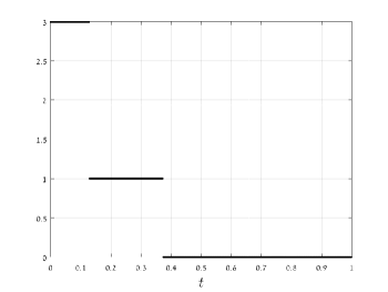
Figure 1: $\sigma(z(t))$ as a function of $t$ for the system in Example 16.

Thm. 5 implies that if $\dot{z}=Az$ is TPDS on $(a,b)$ then the combined number of zeros of $z_{1}(t)$ and $z_{n}(t)$ on $(a,b)$ does not exceed $n-1$. A natural question is whether the number of zeros of other entries of the vector $z(t)$ is also bounded.

Consider first the case where $A\in\mathbb{M}^{+}$ is a constant matrix. Then there exists $r\geq 0$ such that $B:=rI+A$ is TN (by the result in Example 3), irreducible, and non-singular. Thus, $B$ is oscillatory, and applying Thm. 1 we conclude that all the eigenvalues of $A$ are real and can be ordered as $\lambda_{1}>\lambda_{2}>\dots>\lambda_{n}$. Any nontrivial solution of $\dot{z}=Az$ has the form $z(t)=\sum_{i=1}^{n}c_{i}\exp(\lambda_{i}t)u^{i},$ where the $c_{i}$s are not all zero. This implies that any entry of $z(t)$ has no more than $n-1$ isolated zeros on any time interval.

On the other-hand, the next example from Schwarz (1970) shows that if $A(t)$ is time-varying then some entries of the TPDS $\dot{z}=Az$ may have an unbounded number of zeros.

Example 17.

Consider (19) with $n=3$ and $A(t)=\begin{bmatrix}0&1&0\\ \frac{3}{2}-\cos(t)&0&\frac{3}{2}+\cos(t)\\ 0&1&0\end{bmatrix}$. Note that $A(t)\in\mathbb{M}^{+}$ for all $t$, so the system is TPDS on any interval $(a,b)$. Note that $z(t)=\begin{bmatrix}2+\cos(t)&-\sin(t)&-2+\cos(t)\end{bmatrix}^{\prime}$ is a solution of (19) and that $z_{2}(t)$ changes sign an unbounded number of times. Note also that $z(t)\in\mathcal{V}$ and $\sigma(z(t))=1$ for all $t$.

3.1 The periodic case

If $\dot{x}=f(x)$ admits a solution $\phi(t)$ that is periodic with period $T$ then $z:=\dot{\phi}$ satisfies $\dot{z}(t)=J(\phi(t))z(t)$, and thus the matrix here is also periodic with period $T$. Analysis of the time-varying periodic linear system can provide considerable information on the periodic trajectory of the nonlinear system (see, e.g. Mallet-Paret and Smith (1990) and the references therein).

In this section, we thus consider the TPDS $\dot{z}=A(t)z$, $z(t_{0})=z_{0}$, with the additional assumption that $A(t)$ is $T$-periodic, i.e.

$$A(t)=A(t+T),\quad\text{for all }t.$$ (27)

We recall some known results from Floquet theory (see e.g. (Chicone, 1999, Ch. 2)). For simplicity, we assume from hereon that $t_{0}=0$, and write $\Phi(t)=\Phi(t,0)$ for the solution of (18) at time $t$. Let $B:=\Phi(T)$. Then $\Phi(t+T)=\Phi(t)B$ for all $t\geq 0$. The eigenvalues of $B$ are called the characteristic multipliers of (18). If $\alpha\in\mathbb{C}$, $u\in\mathbb{C}^{n}$ is an eigenvalue/eigenvector pair of $B$ then $z(t):=\Phi(t)u$ is a solution of $\dot{z}=A(t)z$, and $z(t+T)=\alpha z(t)$. If $s\in\mathbb{C}$ is such that $\exp(sT)=\alpha$ then defining $q(t):=\exp(-st)z(t)$ yields $z(t)=\exp(st)q(t)$, and $q(t+T)=q(t)$.

Since the system is TPDS, $B=\Phi(T)$ is TP. Let $\alpha_{k}\in\mathbb{C},p^{k}\in\mathbb{C}^{n}$, $k=1,\dots,n$, denote the eigenvalues and corresponding eigenvectors of $B$. Thm. 1 implies that the eigenvalues are real and satisfy $\alpha_{1}>\alpha_{2}>\dots>\alpha_{n}>0,$ i.e., all the characteristic multipliers are real, positive, and distinct. The corresponding eigenvectors satisfy $s^{-}(p^{k})=s^{+}(p^{k})=k-1$ for all $k$. The next result shows that this induces a strong structure on the solutions of the periodic time-varying linear system.

Theorem 9.

Suppose that $A(t)$ satisfies (27) and that $\dot{\Phi}=A\Phi$ is TPDS on $(0,T)$. Pick $1\leq i\leq j\leq n$ and $c_{i},\dots c_{j}\in\mathbb{R}$, with $c_{i}\not=0$. Then the solution of $\dot{z}=A(t)z$, $z(0)=\sum_{k=i}^{j}c_{k}p^{k}$, satisfies

$$i-1\leq\sigma(z(t))\leq j-1,$$ (28)

for all $t\geq 0$ except, perhaps, for up to $j-i$ isolated points, and $\sigma(z(t))=i-1$ for all $t$ sufficiently large. In particular, if $z(0)=c_{i}p^{i}$, with $c_{i}\not=0$, then $\sigma(z(t))\equiv i-1$ for all $t\geq 0$.

Thus, the eigenvectors of $\Phi(T)$ induce a decomposition of the state-space with respect to $\sigma$. The monotonicity of $\sigma$ then restricts the possible dynamics; see Wang and Zhou (2015); Fang et al. (2013).

Proof of Thm. 9. By Thm. 1,

$$i-1\leq s^{-}(z(0))\leq s^{+}(z(0))\leq j-1,$$

and TPDS implies that

$$s^{-}(z(t))\leq s^{+}(z(t))\leq j-1.$$ (29)

To proceed, note that $z(t)=\Phi(t)(\sum_{k=i}^{j}c_{k}p^{k})$ implies that

$$z(t+T) =\Phi(t+T)(\sum_{k=i}^{j}c_{k}p^{k})$$

$$=\Phi(t)B(\sum_{k=i}^{j}c_{k}p^{k})$$

$$=\Phi(t)(\sum_{k=i}^{j}c_{k}\alpha_{k}p^{k}),$$

and iterating this yields $z(mT)=\sum_{k=i}^{j}c_{k}(\alpha_{k})^{m}p^{k}$, for any integer $m\geq 0$. Since $\alpha_{i}>\alpha_{s}$ for all $s>i$, this implies that $\sigma(z(mT))=\sigma(p^{i})=i-1$ for any sufficiently large $m$. Combining this with (29) and using the fact that the system is TPDS, we conclude that

$$i-1\leq s^{-}(z(t))\leq s^{+}(z(t))\leq j-1,\quad\text{for all }t\geq 0,$$

and this proves that (28) holds for all $t\geq 0$ except, perhaps, for up to $j-i$ isolated points.

In the particular case, $z(0)=c_{i}p_{i}$, with $c_{i}\not=0$, (28) yields

$$i-1\leq\sigma(z(t))\leq i-1,$$

for almost all $t\geq 0$ and using monotonicity implies that $\sigma(z(t))\equiv i-1$.  $\square$

Example 18.

Consider the case $n=2$ and $A(t)=\begin{bmatrix}0&1+\sin(t)\\ 1+\sin(t)&0\end{bmatrix}.$ Note that this is $2\pi$-periodic and yields a TPDS on any interval $(a,b)$. The solution of (18) is $\Phi(t)=\begin{bmatrix}\cosh(a(t))&\sinh(a(t))\\ \sinh(a(t))&\cosh(a(t))\end{bmatrix},$ where $a(t):=1+t-\cos(t)$, so $B:=\Phi(2\pi)=\begin{bmatrix}\cosh(2\pi)&\sinh(2\pi)\\ \sinh(2\pi)&\cosh(2\pi)\end{bmatrix}.$ The eigenvalues of $B$ are $\alpha_{1}=\exp(2\pi)$, $\alpha_{2}=\exp(-2\pi)$ and the corresponding eigenvectors are $p^{1}=\begin{bmatrix}1&1\end{bmatrix}^{\prime}$ and $p^{2}=\begin{bmatrix}-1&1\end{bmatrix}^{\prime}$. Note that $\sigma(p^{1})=0$ and $\sigma(p^{2})=1$. Consider $z(t)$ for $z(0)=c_{1}p^{1}+c_{2}p^{2}$ with $c_{1}=1$ and $c_{2}=10$. Then $\sigma(z(0))=1$. For large $t$, $\Phi(t)\approx\frac{1}{2}\exp(a(t))J_{2}$, were $J_{2}$ is the $2\times 2$ matrix with all entries equal to one, and thus $z(t)\approx c_{1}\exp(a(t))\begin{bmatrix}1&1\end{bmatrix}^{\prime}$. We conclude that $\sigma(z(t))=0$ for all sufficiently large $t$.

Schwarz considered only linear time-varying systems. In the next section, we describe how the TPDS framework can be used to analyze the stability of nonlinear dynamical systems.

4 Applications to stability analysis

Consider the nonlinear time-varying dynamical system

$$\dot{x}(t)=f(t,x(t)),$$ (30)

whose trajectories evolve on an invariant set $\Omega\subset\mathbb{R}^{n}$, that is, for any $x_{0}\in\Omega$ and any $t_{0}\geq 0$ a unique solution $x(t,t_{0},x_{0})$ exists and satisfies $x(t,t_{0},x_{0})\in\Omega$ for all $t\geq t_{0}$. From here on we take $t_{0}=0$. We assume that $\Omega$ is compact and convex, and that $f$ is $C^{1}$ with respect to $x$.

Assumption 1.

For any $t\geq 0$ and along any line $\gamma:[0,1]\to\Omega$ the matrix

$$A(t):=\int_{0}^{1}J(t,\gamma(r))\mathop{}\!\mathrm{d}r$$ (31)

is well-defined, locally (essentially) bounded, measurable, and $\dot{\Phi}(t)=A(t)\Phi(t)$ is TPDS. Here $J(t,x):=\frac{\partial}{\partial x}f(t,x)$ is the Jacobian of the dynamics.

Note that Theorem 8 can be used to establish conditions on $J$ guarantying the required TPDS property.

The next result shows that under Assumption 1 the system (30) satisfies an “eventual monotonicity” property.

Lemma 3.

Pick $a,b\in\Omega$, with $a\not=b$, and consider the solutions $x(t,a)$, $x(t,b)$ of (30). There exists a time $s\geq 0$ such that for all $t\geq s$ either $x_{1}(t,a)>x_{1}(t,b)$ or $x_{1}(t,a)<x_{1}(t,b)$.

Proof of Lemma 3. Denote the line between the two solutions at time $t$ by

$$\gamma(r):=rx(t,a)+(1-r)x(t,b),\quad r\in[0,1].$$

Since $\Omega$ is convex, $\gamma(r)\in\Omega$ for all $t\geq 0$ and all $r\in[0,1]$. Let $z(t):=x(t,a)-x(t,b)$. Then

$$\dot{z}(t) =f(t,x(t,a))-f(t,x(t,b))$$

$$=\int_{0}^{1}\frac{d}{dr}f(t,\gamma(r))\mathop{}\!\mathrm{d}r$$

$$=A(t)z(t),$$

with $A(t)$ defined in (31). By assumption, this is TPDS, so Thm. 5 yields $z(t)\in\mathcal{V}$ for all $t$ except for up to $n-1$ time points. In particular, there exists $s\geq 0$ such that $z_{1}(t)\not=0$ for all $t\geq s$.  $\square$

We consider from hereon the case where $f$ is $T$-periodic for some $T>0$.

Assumption 2.

$$f(t,z)=f(t+T,z),\text{ for all }z\in\Omega\text{ and }t\geq 0.$$

Note that in the particular case where $f$ is time-invariant this property holds for all $T$. Note also that this implies that the matrix $A(t)$ in (31) is also $T$-periodic. A solution $\gamma(t)$ of (30) is called a $T$-periodic trajectory if $\gamma(t+T)=\gamma(t)$ for all $t$.

Theorem 10.

If Assumptions 1 and 2 hold then every solution of (30) converges to a $T$-periodic trajectory.

This result has been derived by Smith (1991) based on a direct analysis of the number of sign variations in the vector of derivatives $z(t):=\dot{x}(t)$. In the particular case where $f(t,x)=g(x,u)$, with $u(t)$ $T$-periodic, one may view $u$ as a periodic excitation. Then Thm. 10 implies that the system entrains to the excitation in the sense that every solution converges to a periodic solution with the same period as the excitation. Entrainment is important in many natural and artificial systems. For example, proper functioning of biological organisms often requires entraining of various processes to periodic excitations like the 24h solar day or the cell-division cycle (Russo et al., 2010; Margaliot et al., 2014). Epidemics of infectious diseases often correlate with seasonal changes and interventions like pulse vaccination may also need to be periodic (Grassly and Fraser, 2006; Margaliot et al., 2018).

It is well-known that the linear system $\dot{x}=Ax+Bu$, with $A$ Hurwitz, entrains to a periodic input. More generally, contractive systems entrain (see e.g. Coogan and Margaliot (2018)). However, nonlinear systems do not necessarily entrain. There are examples of “innocent looking” nonlinear dynamical systems that generate chaotic trajectories when excited with periodic inputs (Nikolaev et al., 2018).

The next example, which is a special case of a construction from Takáč (1992), shows that even strongly cooperative systems do not necessarily entrain.

Example 19.

Consider the system

$$\dot{x}=\begin{bmatrix}1&0&0&1\\ 1&1&0&0\\ 0&1&1&0\\ 0&0&1&1\end{bmatrix}x+\begin{bmatrix}-2x_{1}^{3}+x_{1}u\\ -2x_{2}^{3}-x_{2}u\\ -2x_{3}^{3}+x_{3}u\\ -2x_{4}^{3}-x_{4}u\end{bmatrix}.$$ (32)

Note that this is a strongly cooperative system, but not a tridiagonal system because of the feedback connection from $x_{4}$ to $x_{1}$. For $u(t)=\cos(2t)$ it is straightforward to verify that $\gamma(t):=\begin{bmatrix}\cos(t)&\sin(t)&-\cos(t)&-\sin(t)\end{bmatrix}^{\prime}$ is a solution of (32). Furthermore, it can be shown that this solution is locally asymptotically stable (Takáč, 1992). Thus, for an excitation that is periodic with period $T=\pi$ there exist trajectories converging to $\gamma$ that are periodic with a minimal period $2T$.

We can now prove Thm. 10. Pick $a\in\Omega$. If the solution $x(t,a)$ of (30) is $T$-periodic then there is nothing to prove. Thus, suppose that $x(t,a)$ is not $T$-periodic. Then $x(t+T,a)$ is another solution of (30) that is different from $x(t,a)$. Using Lemma 3 we conclude that there exists an integer $m\geq 0$ such that $x_{1}(kT,a)-x_{1}((k+1)T,a)\not=0$ for all $k\geq m$. Without loss of generality, assume that

$$x_{1}(kT,a)-x_{1}((k+1)T,a)>0\text{ for all }k\geq m.$$ (33)

Define the Poincaré map $P_{T}:\Omega\to\Omega$ by $P_{T}(y):=x(T,y).$ Then $P_{T}$ is continuous, and for any integer $k\geq 1$ the $k$-times composition of $P_{T}$ satisfies $P_{T}^{k}(y)=x(kT,y)$. The omega limit set $\omega_{T}:\Omega\to\Omega$ is defined by

$$\omega_{T}(y):= \{z\in\Omega:\text{ there exists a sequence }n_{1},n_{2},\dots$$

$$\text{ with }n_{k}\to\infty\text{ and }\lim_{k\to\infty}P_{T}^{n_{k}}(y)=z\}.$$

This set is not empty, invariant under $P_{T}$, that is, $P_{T}(\omega_{T}(y))=\omega_{T}(y)$, and $P_{T}^{n}(y)\to\omega_{T}(y)$ as $n\to\infty$. In particular, if $\omega_{T}(y)=\{q\}$ then $P_{T}(q)=q$, that is, the solution emanating from $q$ is $T$-periodic. Thus, to prove the theorem we need to show that $\omega_{T}(a)$ is a singleton. Assume that this is not the case. Then there exist $p,q\in\omega_{T}(a)$ with $p\not=q$. This means that there exist integer sequences $n_{k}\to\infty$ and $m_{k}\to\infty$ such that

$$\lim_{k\to\infty}x(n_{k}T,a)=p,\quad\lim_{k\to\infty}x(m_{k}T,a)=q.$$

Without loss of generality, we may pick $n_{k}<m_{k}<n_{k+1}$ for all $k$, which implies by (33) that $x_{1}(n_{k}T,a)<x_{1}(m_{k}T,a)<x_{1}(n_{k+1}T,a)$ for all $k$ sufficiently large, which passing to the limit yields $p_{1}=q_{1}$. In other words, any two points $p,q\in\omega_{T}(a)$ have the same first coordinate. Consider the solutions emanating from $p$ and from $q$ at time zero, that is, $x(t,p)$ and $x(t,q)$. We know that there exists an integer $m\geq 0$ such that, say,

$$x_{1}(kT,p)-x_{1}(kT,q)>0\text{ for all }k\geq m.$$ (34)

But since $p,q\in\omega_{T}(a)$, $x(kT,p),x(kT,q)\in\omega_{T}(a)$ for all $k$, and this means that $x(kT,p)$ and $x(kT,q)$ have the same first coordinate. This contradiction completes the proof of Thm. 10.  $\square$

The time-invariant nonlinear dynamical system:

$$\dot{x}(t)=f(x(t))$$ (35)

is $T$-periodic for all $T>0$, so Thm. 10 yields the following result.

Corollary 1.

Suppose that: (1) the solutions of (35) evolve on an invariant compact and convex set $\Omega\subset\mathbb{R}^{n}$; (2) $f\in C^{1}$; and (3) the matrix $J(x):=\frac{\partial}{\partial x}f(x)\in\mathbb{M}^{+}$ for all $x\in\Omega$. Then for every $x_{0}\in\Omega$ the solution $x(t,x_{0})$ converges to an equilibrium point.

This is a generalization of Smillie’s theorem. Indeed, the proof in Smillie (1984) is based on studying $\sigma(z(t))$ near zeros of the $z_{i}$s and since these may be high-order zeros, Smillie used iterative differentiations and thus had to assume that every entry $f_{i}$ of the vector field is $(n-1)$-times differentiable (Smillie, 1984, p. 530).

Note that the approach used by Smillie provides a sufficient condition for the dynamical system $\dot{z}=Az$ to satisfy (21) for all $a<t_{0}<t<b$ and all $z(t_{0})\in\mathbb{R}^{n}\setminus\{0\}$, but it seems difficult to use this approach to understand if this is also a necessary condition. Remark 2 above shows that the TPDS approach solves this question.

5 Directions for future research

We believe that one of the most important implications of this paper is that it opens many new and interesting research directions. We now briefly describe several such potential directions.

First, the elegant proofs of Schwarz from 1970 are based on what is now known as the theory of cooperative dynamical systems. But since then this theory has been greatly developed. Extensions include for example cooperative systems in canonical form (Smith, 2012), the theory of monotone (rather than cooperative) systems, and the new notion of monotone control systems (Angeli and Sontag, 2003). These extensions can perhaps yield new and interesting results in the context of TPDS.

Second, the direct proof of the SVDP in the work of Smillie and others is difficult to generalize to other cases. Using the connection to TPDS suggests an easier track for generalizing these results to other forms of dynamical systems, for example, those with transition operators that have an SVDP. Note that there is a large body of work on kernels satisfying an SVDP (see, e.g. Karlin (1968); Pinkus (1996)). Another possible direction is motivated by weakening the requirement of TPDS to TNDS. Note that the proof of Thm. 10 mainly uses the eventual monotonicity behavior of the first entry of the solution $z$ in a TPDS $\dot{z}=Az$ described in Lemma 3. In a TNDS, this property does not hold. Yet, Schwarz showed that a weaker property does hold.

Lemma 4.

(Schwarz, 1970) Suppose that $\dot{z}=Az$ is a TNDS on $(a,b)$ and that there are times $r,s$ with $a<r<s<b$ such that $z_{1}(r)=0$ and $z_{1}(s)\not=0$. Then

$$s^{+}(z(s))\leq s^{+}(z(r))-1.$$ (36)

Thus, TNDSs do not satisfy the eventual monotonicity described in Lemma 3, but do satisfy the “non-oscillatory” condition described in Lemma 4. The question then is whether it is possible to use this to generalize the results in the TPDS case to TNDS with some additional properties.

Another natural direction for further research is to study the time-discretized solutions of TNDSs. For example, consider a matrix $A\in\mathbb{M}^{+}$. A simple discretization of $\dot{x}=Ax$ is given by $\tilde{z}(k+1)=\tilde{z}(k)+hA\tilde{z}(k),$ with $h>0$. For any $h>0$ sufficiently small it follows from Example 3 that the matrix $I+hA$ is TN. It is also nonsingular, so

$$s^{-}(\tilde{z}(k+1))\leq s^{-}(\tilde{z}(k)),\;\;s^{+}(\tilde{z}(k+1))\leq s^{+}(\tilde{z}(k)),$$

for all $k$. A similar result holds for more sophisticated discretization schemes, say when $A(t)$ is time-varying and $z(k+1)=z(k)+(\int A(s)\mathop{}\!\mathrm{d}s)z(k)$ with integration on an appropriate time interval. An interesting question is what can be deduced from these SVDPs on the asymptotic behavior of the discrete-time systems.

The notion of a TPDS may be useful also for studying nonlinear time-varying, yet not necessarily periodic, dynamical systems. Indeed, consider the system $\dot{x}=f(t,x)$, and suppose that the corresponding variational system $\dot{z}=J(t,x)z$ is TPDS. Then $z(t)\in\mathcal{V}$ for all $t$ except perhaps for up to $n-1$ time points, so in particular there exists a time $s$ such that $z_{1}(t)\not=0$ for all $t\geq s$. This means that $x_{1}(t)$ is monotone for all $t\geq s$. If the state-variables are bounded (and this is typical for example in models from systems biology) then $x_{1}(t)$ converges to a limit $e_{1}$. Similarly, $x_{n}(t)\to e_{n}$. We may now view $x_{2}(t),\dots,x_{n-1}(t)$ as a system of $n-2$ state-variables with “inputs” $x_{1}(t),x_{n}(t)$ that converge to a constant value. If this system admits the converging input converging state (CICS) property (see, e.g., Ryan and Sontag (2006) and the references therein) then we can deduce convergence to equilibrium of the entire state $x(t)$.

We note in passing that the fact that $x_{1}(t),x_{n}(t)$ converge to a limit is interesting by itself especially if these are the system outputs e.g. they feed another “downstream” system.

Another direction for further research is exploring the applications of TPDS to differential analysis and contraction theory (Aminzare and Sontag, 2014; Forni and Sepulchre, 2014; Lohmiller and Slotine, 1998). To explain this, assume that the trajectories of

$$\dot{x}=f(t,x)$$ (37)

evolve on a compact and convex state-space $\Omega$. For $a,b\in\Omega$, let $\gamma(r):=ra+(1-r)b$, with $r\in[0,1]$, denote the line connecting $a$ and $b$, and let $w(t,r):=\frac{\partial}{\partial r}x(t,t_{0},\gamma(r)),$ that is, the change in the solution at time $t$ w.r.t. a change in the initial condition along the line $\gamma$ at the initial time $t_{0}$. Then (see e.g. Russo et al. (2010))

$$\dot{w}(t,r)=J(t,x(t,t_{0},\gamma(r)))w(t,r).$$

This is again a linear time-varying system. If it is TPDS then one can obtain strong results on the asymptotic behaviour of (37) using the SVDP. This idea has already been used extensively by Mallet-Paret and Smith (1990); Fusco and Oliva (1990) and others, but using direct analysis of the evolution of the number of sign changes in $w$. The relation to TPDS may lead to new results.

Another topic for further research is based on the fact that several authors used a slightly different notion of the number of sign variations as a discrete-valued Lyapunov function. For a vector $x\in\mathbb{R}^{n}$ with no zero entries let $\sigma_{c}(x):=|\{i\in\{1,\dots,n\}:x_{i}x_{i+1}<0\}|$, where $x_{n+1}:=x_{1}$. This is the “cyclic” number of sign changes in $x$. The results in Fusco and Oliva (1990); Smith (1990) show that for some linear dynamical systems $\sigma_{c}(z(t))$ can only decrease along any solution $z(t)$. The proofs are based on direct calculations. Recall that the SVDP with respect to the “standard” number of sign variations $\sigma$ characterizes the sign-regular matrices. This leads to the following question: when does $A$ (and $\exp(At)$) satisfies an SVDP with respect to $\sigma_{c}$?

6 Conclusions

TN and TP matrices enjoy a rich set of powerful properties and have found applications in numerous fields. A natural question is when is the transition matrix of a linear dynamical system $\dot{z}=Az$ TN or TP? This problem has been solved by Schwarz (1970) yielding the notion of TNDS and TPDS. One important property of such systems is that for any solution $z(t)$ the number of sign variations $\sigma(z(t))$ is non-increasing with time. His approach is based on what is now known as cooperative systems theory: a system is TNDS [TPDS] if all the minors of the transition matrix, that are all either zero or one at the initial time $t_{0}$, are non-negative [positive] for all $t>t_{0}$. However, the seminal work of Schwarz has been largely forgotten, perhaps because he did not show how to apply these results to analyze non-linear dynamical systems.

More recently, the number of sign changes $\sigma(z(t))$, where $z:=\dot{x}$, has been used by several authors as an integer-valued Lyapunov function for the nonlinear system $\dot{x}=f(t,x)$. In these works, the fact that $\sigma(z(t))$ is non-increasing with time has been proved by a direct and sometimes tedious analysis.

In this paper, we reviewed these seemingly different lines of research and showed that the linear time-varying system describing the evolution of $z$ (i.e., the variational system) is in fact TPDS. Our results allow to derive important generalizations to several known results, while greatly simplifying the proofs. We hope that the expository nature of this paper will make these fascinating topics accessible to a large audience as well as open the door to many new and interesting research directions.

Acknowledgments: We thank the anonymous referees and the Editor for their constructive comments. The first author is grateful to George Weiss, Yoram Zarai, Guy Sharon, Tsuff Ben Avraham, Lars Grüne, and Thomas Kriecherbauer for many helpful comments.

Appendix: SVDP of square sign-regular matrices

In this Appendix, we review the SVDP of square sign-regular matrices. We follow the presentation in (Gantmacher and Krein, 2002, Ch. V), as this requires little more than basic manipulations of determinants. We begin with an auxiliary result that provides information on the number of sign changes in a vector obtained as a linear combination of $m$ given vectors.

Proposition 1.

Consider a set of $m$ vectors $u^{1},\dots,u^{m}\in\mathbb{R}^{n}$, with $m<n$. Define the matrix $U\in\mathbb{R}^{n\times m}$ by $U:=\begin{bmatrix}u^{1}&u^{2}&\dots&u^{m}\end{bmatrix}.$ The following two conditions are equivalent:

1. For any $c_{1},\dots,c_{m}\in\mathbb{R}$, that are not all zero,

   $$s^{+}(\sum_{k=1}^{m}c_{i}u^{i})\leq m-1.$$ (38)

2. All the minors of order $m$ of $U$, that is, all minors of the form

   $$U(i_{1}\;\dots\;i_{m}|1\;\dots\;m),\text{ with }1\leq i_{1}<\dots<i_{m}\leq n,$$ (39)

   are non-zero and have the same sign.

Remark 4.

Note that if $m=n$ then condition (1) always holds, whereas condition (2) holds iff $U$ is non-singular. Thus, the proposition does not hold in the case $m=n$.

Example 20.

Consider the TP matrix in Example 5. Its first two eigenvectors are $u^{1}=\begin{bmatrix}1&\sqrt{2}&1\end{bmatrix}^{\prime}$, and $u^{2}=\begin{bmatrix}-1&0&1\end{bmatrix}^{\prime}$. We know from Thm. 1 that for any $c_{1},c_{2}\in\mathbb{R}$, that are not both zero, $s^{+}(c_{1}u^{1}+c_{2}u^{2})\leq 1,$ that is, condition (1) holds. In this case, $U=\begin{bmatrix}1&-1\\ \sqrt{2}&0\\ 1&1\end{bmatrix}$, and thus the minors in (39) are $\det(\begin{bmatrix}1&-1\\ \sqrt{2}&0\end{bmatrix})$, $\det(\begin{bmatrix}1&-1\\ 1&1\end{bmatrix})$, $\det(\begin{bmatrix}\sqrt{2}&0\\ 1&1\end{bmatrix})$. These are all positive, so condition (2) also holds.

Proof of Prop. 1. It is enough to prove the result for the case $n=m+1$ (the proof when $n>m+1$ is similar).

We first show that condition (2) implies condition (1). Suppose that all the minors in (39) are non-zero and have the same sign. Pick $c_{1},\dots,c_{m}\in\mathbb{R}$, that are not all zero, and let $u:=\sum_{i=1}^{m}c_{i}u^{i}\in\mathbb{R}^{m+1}$. We need to show that $s^{+}(u)\leq m-1$. Seeking a contradiction, assume that $s^{+}(u)\geq m$. This means that

$$u_{i}u_{i+1}\leq 0\text{ for }i=1,\dots,m.$$ (40)

Furthermore, condition (2) implies that at least one of the first $m$ entries of $u$ is not zero. Consider the square matrix $V:=\begin{bmatrix}u&u^{1}&\dots&u^{m}\end{bmatrix}$. Expanding its determinant along the first column and using (40) and condition (2) implies that $\det(V)\not=0$. But, the first column of $V$ is a linear combination of the other columns, so $\det(V)=0$. This contradiction completes the proof that condition (2) implies condition (1).

To prove the converse implication, assume that condition (1) holds. This implies in particular that for any $c_{1},\dots,c_{m}$, that are not all zero, $\sum_{k=1}^{m}c_{i}u^{i}\not=0$, so the $u^{i}$s are linearly independent. Assume that one of the minors in (39) is zero. Then there exist $c_{1},\dots,c_{m}$, not all zero, such that $\sum_{i=1}^{m}c_{k}u^{k}$ has $m$ zero entries. Since $n=m+1$ this means that $s^{+}(\sum_{i=1}^{m}c_{k}u^{k})\geq m$ and this is a contradiction. We conclude that all the minors of order $m$ are not zero. To prove that they all have the same sign it is enough to prove that all the minors

$$d_{k}:=U(1\;\dots\;k-1\;k+1\;\dots\;m+1|1\;\dots\;m),$$

with $k=1,\dots,m+1,$ have the same sign. Fix $1\leq i<j\leq m+1$. Define a vector $z\in\mathbb{R}^{m+1}$ by

$$z_{k}:=\begin{cases}(-1)^{i-1}d_{j}&\text{if }k=i,\\ (-1)^{j}d_{i}&\text{if }k=j,\\ 0&\text{otherwise.}\end{cases}$$

Consider the square matrix $V:=\begin{bmatrix}u^{1}&\dots&u^{m}&z\end{bmatrix}$. Expanding its determinant along the last column yields $\det(V)=0$. Thus, there exist $c_{1},\dots,c_{m+1}$, not all zero, such that

$$v :=\sum_{k=1}^{m}c_{k}u^{k}$$ (41)

$$=-c_{m+1}z.$$

If $c_{1}=\dots=c_{m}=0$ then this gives $z=0$, but this is a contradiction as $d_{j},d_{i}\not=0$. Thus, at least one of $c_{1},\dots,c_{m}$ is not zero. If $c_{m+1}=0$ then (41) yields $\sum_{k=1}^{m}c_{k}u^{k}=0$ and this contradicts condition (1). We conclude that $c_{m+1}\not=0$, and we assume from here on that $c_{m+1}=1$, so

$$v=-z.$$ (42)

Let $\alpha:=\operatorname{{\mathrm{s}gn}}(d_{j})\in\{-1,1\}$ and let $\bar{v}$ be the vector $v$ but with every zero entry $v_{p}$ replaced by $(-1)^{p}\alpha$. Then by the definition of $s^{+}$, $s^{+}(v)\geq s^{+}(\bar{v})$. Using (42) implies that the entries of $\frac{1}{\alpha}\bar{v}$ are

$$(-1)^{1} ,\;(-1)^{2},\;\dots\;(-1)^{i-1},\;\;\frac{(-1)^{i}}{\alpha}d_{j},\;\;(-1)^{i+1},\dots,$$

$$(-1)^{j-1},\;\;\frac{(-1)^{j-1}}{\alpha}d_{i},\;\;(-1)^{j+1},\dots,(-1)^{m+1}.$$

If $d_{i},d_{j}$ have different signs then we see that $s^{+}(\bar{v})\geq m$, so $s^{+}(v)\geq m$. This contradiction completes the proof that condition (1) implies condition (2).  $\square$

We can now state the main result in this Appendix.

Theorem 11.

Consider a set of $n$ linearly independent vectors $a^{1},\dots,a^{n}\in\mathbb{R}^{n}$. The following two conditions are equivalent:

1. For any vector $c\in\mathbb{R}^{n}\setminus\{0\}$,

   $$s^{+}(\sum_{k=1}^{n}c_{i}a^{i})\leq s^{-}(c).$$ (43)

2. The matrix $A:=\begin{bmatrix}a^{1}&a^{2}&\dots&a^{n}\end{bmatrix}$ is SSR.

Clearly, Thm. 11 is equivalent to Thm. 4.

Proof of Thm. 11. Assume that condition (1) holds. Pick $1\leq p\leq n$. We will show that all minors of order $p$ of $A$ are non-zero and have the same sign. If $p=n$ then this holds because the $a^{i}$s are linearly independent. Thus, consider the case $p<n$. Pick $p+1$ indices $1\leq k_{1}<k_{2}<\dots<k_{p}<k_{p+1}\leq n$. For any $c\in\mathbb{R}^{n}$, define $\bar{c}\in\mathbb{R}^{n}$ by

$$\bar{c}_{i}:=\begin{cases}c_{i}&\text{if }i\in\{k_{1},\dots,k_{p}\},\\ 0&\text{otherwise}.\end{cases}$$

Then $s^{-}(\bar{c})\leq p-1$, as $\bar{c}$ has no more than $p$ non-zero entries. Let $\bar{a}:=\sum_{i=1}^{n}\bar{c}_{i}a^{i}=\sum_{j=1}^{p}c_{k_{j}}a^{k_{j}}$. Applying condition (1) implies that for any $\bar{c}\not=0$, $s^{+}(\bar{a})\leq p-1$. This means that the set $\{a^{k_{1}},\dots,a^{k_{p}}\}$ satisfies condition (1) in Prop. 1. Thus, all minors of the form

$$A(i_{1}\;\dots\;i_{p}|k_{1}\;\dots\;k_{p}),\text{ with }1\leq i_{1}<\dots<i_{p}\leq n,$$ (44)

are non-zero and have the same sign. Denote this sign by $\varepsilon(k_{1},\dots,k_{p})$. It remains to show that this sign depends on $p$, but not on the particular choice of $k_{1},\dots,k_{p}$. Pick $v\in\{1,\dots,p\}$. We will show that

$$\varepsilon (k_{1},\dots,k_{v-1},k_{v+1},\dots,k_{p+1})$$

$$=\varepsilon(k_{1},\dots,k_{v},k_{v+2},\dots,k_{p+1}).$$ (45)

To do this, define $p$ vectors $\bar{a}^{k_{1}},\dots,\bar{a}^{k_{v}},\bar{a}^{k_{v+2}},\dots,\bar{a}^{k_{p+1}}$ by $\bar{a}^{k_{i}}:=a^{k_{i}}$ for $i\in\{1,\dots,v-1,v+2,\dots,p+1\}$, and $\bar{a}^{k_{v}}:=d_{v}a^{k_{v}}+d_{v+1}a^{k_{v+1}}$, where $d_{v},d_{v+1}>0$. Pick $\bar{c}_{1},\dots,\bar{c}_{v},\bar{c}_{v+2},\dots,\bar{c}_{p+1}$, that are not all zero, and let

$$a:=\sum_{\genfrac{}{}{0.0pt}{}{i=1}{i\not=v+1}}^{p+1}\bar{c}_{i}\bar{a}^{k_{i}}.$$ (46)

Then

$$a=\sum_{i=1}^{p+1}g_{i}a^{k_{i}},$$ (47)

with $g_{v}:=\bar{c}_{v}d_{v}$, $g_{v+1}:=\bar{c}_{v}d_{v+1}$, and $g_{i}=\bar{c}_{i}$ for all other $i$. Let $g:=\begin{bmatrix}g_{1}&\dots&g_{p+1}\end{bmatrix}^{\prime}$. Note that $g\not=0$, and that since $g_{v}g_{v+1}=(\bar{c}_{v})^{2}d_{v}d_{v+1}\geq 0$, $s^{-}(g)\leq p-1$. Applying condition (1) to (47) yields $s^{+}(a)\leq s^{-}(g)=p-1$, that is,

$$s^{+}(\sum_{\genfrac{}{}{0.0pt}{}{i=1}{i\not=v+1}}^{p+1}\bar{c}_{i}\bar{a}^{k_{i}})\leq p-1.$$

Let $\bar{A}\in\mathbb{R}^{n\times p}$ be the matrix

$$\bar{A}: =\begin{bmatrix}\bar{a}^{k_{1}}&\dots&\bar{a}^{k_{v-1}}&\bar{a}^{k_{v}}&\bar{a}^{k_{v+2}}&\dots&\bar{a}^{k_{p+1}}\end{bmatrix}$$

$$=\begin{bmatrix}a^{k_{1}}&\dots&a^{k_{v-1}}&d_{v}a^{k_{v}}+d_{v+1}a^{k_{v+1}}&a^{k_{v+2}}&\dots&a^{k_{p+1}}\end{bmatrix}.$$

Applying Prop. 1 to the set of $p$ vectors $\bar{a}^{k_{1}}$, $\dots$, $\bar{a}^{k_{v}}$, $\bar{a}^{k_{v+2}}$, $\dots$, $\bar{a}^{k_{p+1}}\in\mathbb{R}^{n}$ we conclude that all minors

$$\bar{A}(i_{1},\dots,i_{p}|k_{1},\dots,k_{v},k_{v+2},\dots,k_{p+1})$$

$$=d_{v}A(i_{1},\dots,i_{p}|k_{1},\dots,k_{v},k_{v+2},\dots,k_{p+1})$$

$$+d_{v+1}A(i_{1},\dots,i_{p}|k_{1},\dots,k_{v-1},k_{v+1},\dots,k_{p+1})$$ (48)

are non-zero. This holds for all $d_{v},d_{v+1}>0$, so the two minors on the right hand side of (Appendix: SVDP of square sign-regular matrices) have the same sign. Since this is true for all $v\in\{1,\dots,p\}$, we conclude that the sign $\varepsilon(k_{1},\dots,k_{p})$ does not change if we change any one of the indices $k_{i}$, and thus it is independent of the choice of $k_{1},\dots,k_{p}$. This completes the proof that condition (1) implies condition (2).

To prove the converse implication, assume that $A=\begin{bmatrix}a^{1}&\dots&a^{n}\end{bmatrix}$ is SSR. Pick $c\in\mathbb{R}^{n}\setminus\{0\}$, and let $p:=s^{-}(c)$. If $p=n-1$ then clearly $s^{+}(\sum_{i=1}^{n}c_{i}a_{i})\leq s^{-}(c)$. Consider the case $p<n-1$. We may assume that the first non-zero entry of $c$ is positive. Then $c$ can be decomposed into $p+1$ groups: $(c_{1},\dots,c_{v_{1}})$, $(c_{v_{1}+1},c_{v_{1}+2},\dots,c_{v_{2}})$, $\dots$, $(c_{v_{p}+1},c_{v_{p}+2},\dots,c_{v_{p+1}})$, where $c_{1},\dots,c_{v_{1}}\geq 0$ (with at least one of these entries positive); $c_{v_{1}+1}<0$, $c_{v_{1}+2},\dots,c_{v_{2}}\leq 0$, $c_{v_{2}+1}>0$, and so on. Define vectors $u^{1},\dots,u^{p+1}\in\mathbb{R}^{n}$ by

$$u^{1}:=\sum_{k=1}^{v_{1}}|c_{k}|a^{k},\;u^{2}:=\sum_{k=v_{1}+1}^{v_{2}}|c_{k}|a^{k},\dots.$$

Then

$$a:=\sum_{k=1}^{n}c_{k}a^{k}=u^{1}-u^{2}+u^{3}-\dots+(-1)^{p}u^{p+1}.$$ (49)

Note that every $u^{i}$ is a non-negative and non-trivial sum of a consecutive set of $a^{k}$s. Let $U:=\begin{bmatrix}u^{1}&\dots&u^{p+1}\end{bmatrix}\in\mathbb{R}^{n\times(p+1)}.$ Note that $n>p+1$. The SSR of $A$ implies that all the minors of order $(p+1)$ of $U$ are non-zero and have the same sign. Applying Prop. 1 to (49) yields $s^{+}(a)\leq p$, so $s^{+}(a)\leq s^{-}(c)$.  $\square$

Michael Margaliot received the BSc (cum laude) and MSc degrees in Elec. Eng. from the Technion-Israel Institute of Technology-in 1992 and 1995, respectively, and the PhD degree (summa cum laude) from Tel Aviv University in 1999. He was a post-doctoral fellow in the Dept. of Theoretical Math. at the Weizmann Institute of Science. In 2000, he joined the Dept. of Elec. Eng.-Systems, Tel Aviv University, where he is currently a Professor and Chair. His research interests include the stability analysis of differential inclusions and switched systems, optimal control theory, fuzzy control, computation with words, Boolean control networks, contraction theory, and systems biology. He is co-author of New Approaches to Fuzzy Modeling and Control: Design and Analysis, World Scientific, 2000 and of Knowledge-Based Neurocomputing, Springer, 2009. He served as an Associate Editor of IEEE Transactions on Automatic Control during 2015-2017.

Eduardo Sontag received his Licenciado degree from the Mathematics Department at the University of Buenos Aires in 1972, and his Ph.D. (Mathematics) under Rudolf E. Kalman at the University of Florida, in 1977. From 1977 to 2017, he was with the Department of Mathematics at Rutgers, The State University of New Jersey, where he was a Distinguished Professor of Mathematics as well as a Member of the Graduate Faculty of the Department of Computer Science and the Graduate Faculty of the Department of Electrical and Computer Engineering, and a Member of the Rutgers Cancer Institute of NJ. In addition, Dr. Sontag served as the head of the undergraduate Biomathematics Interdisciplinary Major, Director of the Center for Quantitative Biology, and Director of Graduate Studies of the Institute for Quantitative Biomedicine. In January 2018, Dr. Sontag was appointed as a University Distinguished Professor in the Department of Electrical and Computer Engineering and the Department of BioEngineering at Northeastern University. Since 2006, he has been a Research Affiliate at the Laboratory for Information and Decision Systems, MIT, and since 2018 he has been a member of the Faculty in the Program in Therapeutic Science at Harvard Medical School.

His major current research interests lie in several areas of control and dynamical systems theory, systems molecular biology, cancer and immunology, and computational biology. He has authored over five hundred research papers and monographs and book chapters in the above areas with over 43,000 citations and an h-index of 89. He is in the Editorial Board of several journals, including: IET Proceedings Systems Biology, Synthetic and Systems Biology, International Journal of Biological Sciences, and Journal of Computer and Systems Sciences, and is a former Board member of SIAM Review, IEEE Transactions in Automatic Control, Systems and Control Letters, Dynamics and Control, Neurocomputing, Neural Networks, Neural Computing Surveys, Control-Theory and Advanced Technology, Nonlinear Analysis: Hybrid Systems, and Control, Optimization and the Calculus of Variations. In addition, he is a co-founder and co-Managing Editor of the Springer journal MCSS (Mathematics of Control, Signals, and Systems).

He is a Fellow of various professional societies: IEEE, AMS, SIAM, and IFAC, and is also a member of SMB and BMES. He has been Program Director and Vice-Chair of the Activity Group in Control and Systems Theory of SIAM, and member of several committees at SIAM and the AMS, including Chair of the Committee on Human Rights of Mathematicians of the latter in 1981-1982. He was awarded the Reid Prize in Mathematics in 2001, the 2002 Hendrik W. Bode Lecture Prize and the 2011 Control Systems Field Award from the IEEE, the 2002 Board of Trustees Award for Excellence in Research from Rutgers, and the 2005 Teacher/Scholar Award from Rutgers.

References

- Aminzare and Sontag [2014] Z. Aminzare and E. D. Sontag. Contraction methods for nonlinear systems: A brief introduction and some open problems. In Proc. 53rd IEEE Conf. on Decision and Control, pages 3835–3847, Los Angeles, CA, 2014.
- Angeli and Sontag [2003] D. Angeli and E. D. Sontag. Monotone control systems. IEEE Trans. Automat. Control, 48:1684–1698, 2003.
- Brualdi and Schneider [1983] R. A. Brualdi and H. Schneider. Determinantal identities: Gauss, Schur, Cauchy, Sylvester, Kronecker, Jacobi, Binet, Laplace, Muir, and Cayley. Linear Algebra Appl., 52-53:769–791, 1983.
- Chicone [1999] C. Chicone. Ordinary Differential Equations with Applications. Springer-Verlag, New York, 1999.
- Chua and Roska [1990] L. O. Chua and T. Roska. Stability of a class of nonreciprocal cellular neural networks. IEEE Trans. Circuits and Systems, 37(12):1520–1527, 1990.
- Coogan and Margaliot [2018] S. Coogan and M. Margaliot. Approximating the steady-state periodic solutions of contractive systems. IEEE Trans. Automat. Control, 2018. To appear.
- Donnell et al. [2009] P. Donnell, S. A. Baigent, and M. Banaji. Monotone dynamics of two cells dynamically coupled by a voltage-dependent gap junction. J. Theoretical Biology, 261(1):120–125, 2009.