Bounding Multivariate Trigonometric Polynomials with Applications to Filter Bank Design

Abstract

The extremal values of multivariate trigonometric polynomials are of interest in fields ranging from control theory to filter design, but finding the extremal values of such a polynomial is generally NP-Hard. In this paper, we develop simple and efficiently computable estimates of the extremal values of a multivariate trigonometric polynomial directly from its samples. We provide an upper bound on the modulus of a complex trigonometric polynomial, and develop upper and lower bounds for real trigonometric polynomials. For a univarite polynomial, these bounds are tighter than existing bounds, and the extension to multivariate polynomials is new. As an application, the lower bound provides a sufficient condition to certify global positivity of a real trigonometric polynomial. We use this condition to motivate a new algorithm for multi-dimensional, multirate, perfect reconstruction filter bank design. We demonstrate our algorithm by designing a 2D perfect reconstruction filter bank.

I Introduction

I-A Motivation

Trigonometric polynomials are intimately linked to discrete-time signal processing, arising in problems of controls, communications, filter design, and super resolution, among others. For example, the Discrete-Time Fourier Transform (DTFT) converts a sequence of length $n$ into a trigonometric polynomial of degree $n-1$. Multivariate trigonometric polynomials arise in a similar fashion, as the $d$-dimensional DTFT yields a $d$-variate trigonometric polynomial.

The extremal values of a trigonometric polynomial are often of interest. In an Orthogonal Frequency Division Multiplexing (OFDM) communication system, the transmitted signal is a univariate trigonometric polynomial, and the maximum modulus of this signal must be accounted for when designing power amplifiers [1]. The maximum modulus of a trigonometric polynomial is related to the stability of a control system in the face of perturbations [2]. The maximum gain and attenuation of a Finite Impulse Response (FIR) filter are the maximum and minimum values of a real and non-negative trigonometric polynomial. Unfortunately, determining the extremal values of a multivariate polynomial given its coefficients is NP-Hard [3, 4].

An approximation to the extremal values can be found by discretizing the polynomial and performing a grid search, but this method is sensitive to the discretization level. Instead, one can try to find the extremal values using an optimization-based approach. However, iterative descent algorithms are prone to finding local optima as a generic polynomial is not a convex function. The sum-of-squares machinery provides an alternative approach: extremal values of a polynomial can be found by solving a hierarchy of semidefinite program (SDP) feasibility problems [5, 4, 2]. Truncating the sequence of SDPs provides a lower (or upper) bound to the minimum (or maximum) of the polynomial. However, the size of the SDPs grows exponentially in the number of variables, $d$, and polynomially in the degree, $n$, limiting the applicability of this approach.

In many applications we have access to samples of the polynomial rather than to the coefficients of the polynomial itself. Equally spaced samples of a trigonometric polynomial arise, for instance, when computing the Discrete Fourier Transform (DFT) of a sequence. Given enough samples, the polynomial can be evaluated at any point by periodic interpolation, and thus grid search or optimization-based approaches can still be used; however, the previously described issues of discretization error, local minima, and complexity remain.

In this paper, we derive simple estimates for the extremal values of a multivariate trigonometric polynomial directly from its samples, i.e. with no interpolation step. For a complex polynomial we provide an upper bound on its modulus, while for a real trigonometric polynomial we provide upper and lower bounds. Upper bounds of this style have been derived for univariate trigonometric polynomials– our work provides an extension to the multivariate case. We describe two sample applications that benefit from our lower bound and from the extension to multivariate polynomials.

i) Design of Perfect Reconstruction Filter Banks. A multi-rate filter bank in $d$ dimensions is characterized by its polyphase matrix, $H(z)\in\mathbb{C}^{m\times n}$, where each entry in the matrix is a $d$-variate Laurent polynomial in $z\in\mathbb{C}^{d}$ [6].

Many important properties of the filter bank can be inferred from the polyphase matrix. A filter bank is said to be perfect reconstruction (PR) if any signal can be recovered, up to scaling and a shift, from its filtered form. The design and characterization of multirate filter banks in one dimension is well understood, but becomes difficult in higher dimensions due to the lack of a spectral factorization theorem [7, 8, 9, 10, 11].

The perfect reconstruction condition is equivalent to the strict positivity of the real trigonometric polynomial $p_{H}(\omega)=\det\left(H^{*}(e^{j\omega})H(e^{j\omega})\right)$ [6, 12]. In Section VI, we use our lower bound to develop a new algorithm for the design and construction of multi-dimensional perfect reconstruction filter banks.

ii) Estimating the smallest eigenvalue of a Hermitian Block Toeplitz matrix with Toeplitz Blocks.

Toeplitz matrices describe shift-invariant phenomena and are found in countless applications. Toeplitz matrices model convolution with a finite impulse response filter, and the covariance matrix formed from a random vector drawn from a wide-sense stationary (WSS) random process is symmetric and Toeplitz. An $n\times n$ Toeplitz matrix is of the form

$$X_{n}=\begin{bmatrix}x_{0}&x_{-1}&x_{-2}&\cdots&x_{-n+1}\\ x_{1}&x_{0}&x_{-1}&&\\ x_{2}&x_{1}&x_{0}&&\vdots\\ \vdots&&&\ddots&\\ x_{n-1}&&&\cdots&x_{0}\end{bmatrix},$$ (1)

and a Hermitian symmetric Toeplitz matrix satisfies $x^{*}_{i}=x_{-i}$. Associated with $X_{n}$ is the trigonometric polynomial

$$\hat{x}(\omega)=\sum_{k=-n}^{n}x_{k}e^{j\omega k},\quad\quad-\pi\leq\omega<\pi,$$ (2)

with coefficients

$$x_{k}=\frac{1}{2\pi}\int_{-\pi}^{\pi}\hat{x}(\omega)e^{-jk\omega}dt,\quad\quad k\in\mathbb{Z}.$$ (3)

The polynomial $\hat{x}$ is known as the symbol of $X_{n}$. If the symbol is real then $X_{n}$ is Hermitian, and if $\hat{x}$ is strictly positive then $X_{n}$ is positive definite.

A vast array of literature has examined the connections between a real symbol $\hat{x}$ and the eigenvalues of the Hermitian Toeplitz matrices $X_{n}$ as $n\to\infty$; see [13, 14] and references therein. One result of particular interest states that the eigenvalues of $X_{n}$ are upper and lower bounded by the supremum and infimum of the symbol.

The smallest eigenvalue of a Toeplitz matrix is of interest in many applications[15, 16, 17], and there are several iterative algorithms to efficiently calculate this eigenvalue [18]. We propose a non-iterative estimate of the smallest and largest eigenvalues of $X_{n}$ by first bounding the eigenvalues in terms of the symbol, then bounding the symbol in terms of the entries of $X_{n}$.

Shift invariant phenomena in two dimensions are described by Block Toeplitz matrices with Toeplitz Blocks (BTTB). The symbol for a BTTB matrix is a bi-variate trigonometric polynomial, and the bounds developed in this paper hold in this case.

I-B Notation

For a set $\mathbb{X}$, let $\mathbb{X}^{d}$ be the $d$-fold Cartesian product $\mathbb{X}\times\ldots\times\mathbb{X}$. Let $\mathbb{T}=[0,2\pi]$ be the torus and $\mathbb{Z}$ be the integers. The set $\left\{0,\ldots N-1\right\}$ is written $\left[N\right]$. We denote the space of $d$-variate trigonometric polynomials with maximum component degree $n$ as

$$T^{d}_{n}\triangleq\mathrm{span}\left\{e^{jk\cdot\omega}:\omega\in\mathbb{T}^{d},k\in\mathbb{Z}^{d},\lVert k\rVert_{\infty}\leq n\right\},$$ (4)

where $x\cdot y\triangleq\sum_{i=1}^{d}x_{i}y_{i}$ is the Euclidean inner product and $\lVert k\rVert_{\infty}=\max_{1\leq i\leq d}\left|k_{i}\right|$. An element of $T_{n}^{d}$ is explicitly given by

$$p(\omega)=\sum_{k_{1}=-n}^{n}\ldots\sum_{k_{d}=-n}^{n}c_{k_{1}\ldots k_{d}}e^{jk_{1}\omega_{1}}\ldots e^{jk_{d}\omega_{d}}.$$ (5)

If the coefficients satisfy $c_{k_{1},\ldots,k_{d}}=c^{*}_{-k_{1},\ldots,-k_{d}}$, then $p(\omega)$ is real for all $\omega$ and $p$ is said to be a real trigonometric polynomial. We denote the space of real trigonometric polynomials by $\bar{T}_{n}^{d}$. For $p\in T_{n}^{d}$ let $\lVert p\rVert_{\infty}=\max_{\omega\in\mathbb{T}^{d}}\left|p(\omega)\right|$. We write the set of $N$ equidistant sampling points on $\mathbb{T}$ as

$$\Theta_{N}\triangleq\left\{\omega_{k}=k\frac{2\pi}{N}:k=0,\ldots,N-1\right\},$$ (6)

and on $\mathbb{T}^{d}$ as $\Theta^{d}_{N}$, given by the $d$-fold Cartesian product $\Theta_{N}\times\ldots\times\Theta_{N}$. The maximum modulus of $p$ over $\Theta^{d}_{N}$ is

$$\lVert p\rVert_{N^{d},\infty}\triangleq\max_{\omega\in\Theta^{d}_{N}}\left|p(\omega)\right|.$$ (7)

I-C Problem Statement and Existing Results

Let $p\in\bar{T}_{n}^{d}$. Our goal is to find scalars $a\leq b$, depending only on $N,d$, and the $N^{d}$ samples $\left\{p(\omega):\omega\in\Theta^{d}_{N}\right\}$, such that

$$a\leq p(\omega)\leq b.$$ (8)

For complex trigonometric polynomials, $p\in T_{n}^{d}$, we want an upper bound on the modulus; a lower bound on the modulus can be obtained by considering the real trigonometric polynomial $p^{\prime}\in\bar{T}_{n}^{2d}:\omega\mapsto\left|p(\omega)\right|^{2}$.

By the periodic sampling theorem (Lemma 1), trigonometric interpolation perfectly recovers $p\in T_{n}^{d}$ from $(2n+1)^{d}$ uniformly spaced samples. A standard result of approximation theory states [19, 20]

$$\lVert p\rVert_{\infty}\leq\lVert p\rVert_{(2n+1)^{d},\infty}\left(\frac{\pi+4}{\pi}+\frac{2}{\pi}\log(2n+1)\right)^{d},$$ (9)

but this becomes weak as the polynomial degree $n$ or the dimension $d$ of its domain increases. A more stable estimate is obtained by using non-uniformly spaced samples. However, in many applications the sampled polynomial is obtained using the DFT, thus providing uniformly spaced samples.

Our aim is to get stronger estimates by using more (uniformly spaced) samples than are required by the periodic sampling theorem. Upper bounds for univariate trigonometric polynomials have been developed using this strategy. Let $p\in T_{n}$. Given an integer $m$ and $N=2m>2n+1$ samples of $p$, Ehlich and Zeller showed

$$\lVert p\rVert_{\infty}\leq\left(\cos{\left(\frac{\pi n}{2m}\right)}\right)^{-1}\lVert p\rVert_{N,\infty}$$ (10)

and this bound is sharp if $n$ is a divisor of $m$.

Wunder and Boche developed a more flexible bound: given $N\geq 2n+1$, they showed [21]

$$\lVert p\rVert_{\infty}\leq\sqrt{\frac{N+2n+1}{N-(2n+1)}}\lVert p\rVert_{N,\infty}.$$ (11)

Zimmermann et al. refined this bound to

$$\lVert p\rVert_{\infty}\leq\frac{\lVert p\rVert_{N,\infty}}{\sqrt{1-\alpha}},$$ (12)

where $\alpha=2n/N$. The quantity $\alpha^{-1}$ is almost equal to the oversampling factor $\frac{N}{2n+1}$, and plays the same role: $\alpha$ is a decreasing function of $N$, and for $N\geq 2n+1$, we have $\alpha<1$.

The bounds 9, 10, 11 and 12 each have the form:

$$\lVert p\rVert_{\infty}\leq C_{N,n}^{d}\lVert p\rVert_{N^{d},\infty},$$ (13)

where $C_{N,n}^{d}$ is a real, non-negative constant that depends on $N,n$ and, in the case of 9, $d$. In the univariate case, Zimmermann et al. studied the optimal value of $C_{N,n}$ and showed that it depends only on $N/n$. They also characterized extremal polynomials, for which 13 holds with equality, and discussed a Remez-like algorithm to construct such polynomials for given $N$ and $n$ [1].

I-D Contributions

Our contributions can be summarized as follows: (i) we develop upper bounds of the form 13 for multivariate trigonometric polynomials; these include both a multivariate extension of the bound (12), as well as a tighter bound for the case of low oversampling ($N\approx 2n+1$); (ii) we specialize and strengthen the bounds for real polynomials; (iii) we derive a lower bound for real trigonometric polynomials; and (iv) we apply our bounds to the design of multi-dimensional perfect-reconstruction filter banks.

II Statement of Main Results

In this section we collect our main results; proofs are deferred to Sections III and IV. For simplicity we work with $T_{n}^{d}$, but the results can be easily strengthened by allowing for the component degree to vary in each of the $d$ dimensions.

Our first task is to obtain bounds of the form 13 for multivariate trigonometric polynomials. We have a pair of such bounds:

Theorem 1.

Let $p\in T_{n}^{d}$. Take $N\geq 2n+1$ and set $\alpha=2n/N$. Then

$$\lVert p\rVert_{\infty}\leq C_{N,n}^{d}\lVert p\rVert_{N^{d},\infty},$$ (14)

where

$$C_{N,n}^{d} \triangleq\frac{\displaystyle\left(\sup_{\omega\in\mathbb{T}}\left\{\sum_{\omega_{k}\in\Theta_{N}}\left|\frac{\sin{\left(\frac{N\omega}{2}\right)}\sin{\left(\frac{N-2n}{2}(\omega-\omega_{k})\right)}}{\sin^{2}{((\omega-\omega_{k})/2)}}\right|\right\}\right)^{d}}{N^{d}(N-2n)^{d}}$$ (15)

$$\leq\left(1-\alpha\right)^{-\frac{d}{2}}.$$ (16)

Further, $C_{N,n}^{d}\lVert p\rVert_{N^{d},\infty}-\lVert p\rVert_{\infty}=\mathcal{O}(dn/N)$.

The bound 15 involves only a univariate function and can be calculated numerically. Still, the expression is unwieldy; 16 is a simpler, but weaker, alternative.

We plot the behavior of $C_{N,n}$, given by 15 and 16 for the $d=1$ univariate case, in Fig. 1. Also shown in Fig. 1 are the optimal values of $C_{N,n}$ for integer oversampling factors, given by 10, and the values obtained using Zimmermann’s Remez-like algorithm [1].

The upper bound 14 with $C_{N,n}^{d}$ given by 15 is nearly tight for $N/(2n)<2$, whereas replacing $C_{N,n}^{d}$ by its upper bound 16 results in a weakening of 14 in this regime. This gap makes 15 particularly attractive in the $d$-variate case, where the bounds are raised to the $d$-th power, further increasing the gap between 15 and 16.

However, for oversampling factor greater than two, i.e. $N/(2n)>2$, the difference in using 15 or 16 becomes negligible. Both bounds coincide with the optimal value at $N=4n$, and are within roughly $10\%$ of the optimal value for large oversampling factors. Hence, both 15 and 16 are useful, in different oversampling regimes.

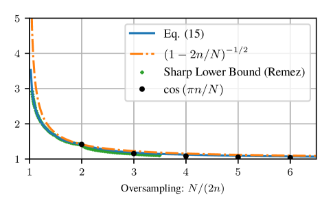
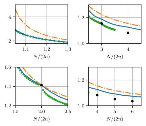
Figure 1: Comparing upper bounds of the form 14 as a function of oversampling ratio, $N/2n$. Green diamonds indicate the optimal upper bound as calculated using a Remez-type algorithm [1, Fig. 2]. Black dots denote the tight upper bound 10 occuring at integer oversampling ratios $N=mn\geq 2n+1$.

Next, we obtain a tighter estimate by restricting our attention to real polynomials.

Corollary 1.

Let $p\in\bar{T}_{n}^{d}$ and take $N\geq 2n+1$. Set $A\triangleq\max_{\omega\in\Theta^{d}_{N}}p(\omega)$, $B\triangleq\min_{\omega\in\Theta^{d}_{N}}p(\omega)$ and take $C_{N,n}^{d}$ as in Theorem 1. Then,

$$\lVert p\rVert_{\infty}\leq\frac{1}{2}\left(A+B+C_{N,n}^{d}\left(A-B\right)\right).$$ (17)

The estimate (17) coincides with (14) in the case that $\min_{\omega\in\Theta^{d}_{N}}p(\omega)=-\max_{\omega\in\Theta^{d}_{N}}p(\omega)$, and is tighter otherwise, making this refinement especially useful for non-negative polynomials.

Using Corollary 1 we obtain the following lower bound:

Corollary 2.

Let $p\in\bar{T}_{n}^{d}$ and take $N\geq 2n+1$. Set $A\triangleq\max_{\omega\in\Theta^{d}_{N}}p(\omega)$, $B\triangleq\min_{\omega\in\Theta^{d}_{N}}p(\omega)$ and take $C_{N,n}^{d}$ as in Theorem 1. Then, for all $\omega\in\mathbb{T}^{d}$,

$$p(\omega)\geq\frac{1}{2}\left(A+B-C_{N,n}^{d}\left(A-B\right)\right).$$ (18)

By Theorem 1, $C_{N,n}^{d}\to 1$ as $N\to\infty$. Thus as $N\to\infty$, the right hand side of 18 approaches $B$, and by continuity we have $B=\min_{\omega\in\Theta^{d}_{N}}p(\omega)\to\min_{\omega\in\mathbb{T}^{d}}p(\omega)$. Thus the bound is tight as $N\to\infty$. In the case of $A=B$, the right hand side of 18 is $A=\lVert p\rVert_{N^{d},\infty}$, and thus $p(\omega)>0$ so long as the samples of $p$ are not uniformly zero. This is expected, as otherwise the polynomial $p(\omega)-\lVert p\rVert_{N^{d},\infty}\in T_{n}^{d}$ would vanish on a set of $N^{d}>(2n+1)^{d}$ points, which is impossible unless the polynomial is identically zero.

A little algebra on 18 establishes a sufficient condition to verify the strict positivity of a multivariate trigonometric polynomial.

Corollary 3.

Let $p\in\bar{T}_{n}^{d}$ and $N\geq 2n+1$. Set $\alpha=2n/N$. If $p(\omega)>0$ for all $\omega\in\Theta^{d}_{N}$ and

$$\kappa_{N}\triangleq\frac{\max_{\omega\in\Theta^{d}_{N}}p(\omega)}{\min_{\omega\in\Theta^{d}_{N}}p(\omega)}\leq\frac{C_{N,n}^{d}+1}{C_{N,n}^{d}-1}$$ (19)

then $p(\omega)>0$ for all $\omega\in\mathbb{T}^{d}$. Furthermore, as $C_{N,n}^{d}\leq\left(1-\alpha\right)^{-\frac{d}{2}}$, 19 can be replaced by the more stringent, but easier to evaluate, condition

$$\kappa_{N}\leq\frac{1+(1-\alpha)^{\frac{d}{2}}}{1-(1-\alpha)^{\frac{d}{2}}}.$$ (20)

For $p\in\bar{T}_{n}^{d}$ with non-negative samples, we call the quantity $\kappa_{N}$ in 19 the N-sample dynamic range; here, $0/0$ is taken to be $1$.

Corollary 3 provides an easy way to certify strict positivity of a real, non-negative polynomial from its samples: simply calculate the dynamic range $\kappa_{N}$ and verify that 19 or 20 holds. These conditions are easier to satisfy (as a function of the oversampling rate) for polynomials whose maximum and minimum sampled values are close to one another. Intuitively, if the sampled values of a real trigonometric polynomial are strictly positive and don’t vary “too much”, then the polynomial is strictly positive over its entire domain. For fixed $n$ and $d$, the right hand sides of 19 and 20 are increasing functions of $N$, illustrating a tradeoff: polynomials with a large amount of variation, and thus large values of $\kappa_{N}$, require larger oversampling factors $N$ for the bounds to hold. Note that $\kappa_{N}$ is not necessarily a monotone function of $N$, but is monotone in $k$ when choosing $N=2^{k}$. Fig. 2 illustrates the regions for which 19 and 20 hold. In Section VI we use this condition to inform the design of multidimensional perfect reconstruction filter banks.

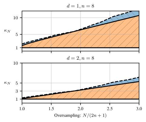
Figure 2: Any $p\in\bar{T}_{n}^{d}$ with positive samples and whose $N$-sample signed dynamic range $\kappa_{N}$ lies in the shaded region must be strictly positive. The orange shaded region is certified using 20, while the blue region uses 19.

III Proof of Theorem 1

We begin by proving Theorem 1, which extends the upper bound (12) from univariate to multivariate polynomials and provides a tighter result for the case of low oversampling. As $T_{n}^{d}$ is constructed as the $d$-fold tensor product of $T_{n}$ with itself, the proof is similar to the follows the univariate case [1]. We consider both real and complex trigonometric polynomials.

III-A Interpolation by the Dirichlet Kernel

For $\mathbf{n}=[n_{1},\ldots n_{d}]\in\left[N\right]^{d}$, the $\mathbf{n}$-th order Dirichlet kernel is the tensor product of $d$ kernels, each of order $n_{i}$:

$$D_{\mathbf{n}}^{d}(\omega)\triangleq\sum_{\left|k_{i}\right|\leq n_{i}}e^{jk\cdot\omega}=\prod_{i=1}^{d}\frac{\sin{\frac{2n_{i}+1}{2}\omega_{i}}}{\sin{\frac{\omega_{i}}{2}}}\quad\omega\in\mathbb{T}^{d},k\in\mathbb{Z}^{d}.$$ (21)

If $\mathbf{n}$ is identical in each index (i.e. $n_{i}=n$ for each $i\in\left[d\right]$) we write the kernel as $D_{n}^{d}(\omega)$. The Dirichlet kernel is key to the periodic sampling formula:

Lemma 1.

Let $p\in T_{n}^{d}$ be sampled on $\Theta^{d}_{N}$. Let $m$ be an integer with $m>n$. If $N\geq n+m$, then

$$p(\omega)=\frac{1}{N^{d}}\sum_{\omega_{k}\in\Theta^{d}_{N}}p(\omega_{k})D^{d}_{m}(\omega-\omega_{k})$$ (22)

for all $\omega\in\mathbb{T}^{d}$.

Lemma 1 (e.g., [22]) is the periodic counterpart of sinc interpolation arising in the Whittaker-Shannon interpolation formula. The bound (9) can be obtained from (22) when $N=2n+1$ [20].

III-B Interpolation by the de la Vallée-Poussin Kernel

A better result is obtained by oversampling $(N>2n+1)$ and exploiting the nice properties of summation kernels.

Let $n,m$ be integers with $m>n$ and define $\mathbb{V}_{n,m}^{d}=\left\{l\in\mathbb{Z}^{d}:n\leq l_{i}<m\right\}$. The $n,m$-th de la Vallée-Poussin kernel is defined as the moving average of Dirichlet kernels:

$$D^{d}_{n,m}(\omega) \triangleq\frac{1}{(m-n)^{d}}\sum_{\ \ \mathclap{\mathbf{n}\in\mathbb{V}^{d}_{n,m}}}D^{d}_{\mathbf{n}}(\omega)$$ (23)

$$=\frac{1}{(m-n)^{d}}\prod_{i=1}^{d}\frac{\sin{(\frac{m+n}{2}\omega_{i})}\sin{(\frac{m-n}{2}\omega_{i})}}{\sin^{2}{(\omega_{i}/2)}}.$$ (24)

Taking $n=0$ recovers the well-known Fejér kernel [23],

$$D^{d}_{0,m}=\frac{1}{m^{d}}\prod_{i=1}^{d}\frac{\sin^{2}{(\frac{m}{2}\omega_{i})}}{\sin^{2}{(\omega_{i}/2)}}.$$ (25)

The Fejér kernel is used to derive the bound 11 [21].

Importantly, the de la Vallée-Poussin kernel inherits the reproducing property of the Dirichlet kernel.

Lemma 2.

For any $p\in T_{n}^{d}$ we have

$$p(\omega)=\frac{1}{N^{d}}\sum_{\omega_{k}\in\Theta^{d}_{N}}p(\omega_{k})D^{d}_{n,m}(\omega-\omega_{k})$$ (26)

for all $\omega\in\mathbb{T}^{d}$ whenever $m>n$ and $N\geq n+m$.

Proof.

Expanding the de la Vallée-Poussin kernel into a sum of Dirichlet kernels and applying Lemma 1,

$$\frac{1}{N^{d}} \sum_{\omega_{k}\in\Theta^{d}_{N}}p(\omega_{k})D^{d}_{n,m}(\omega-\omega_{k})$$ (27)

$$=\frac{1}{(m-n)^{d}}\sum_{{\ \ {\mathbf{n}\in\mathbb{V}^{d}_{n,m}}}}\frac{1}{N^{d}}\sum_{\omega_{k}\in\Theta^{d}_{N}}p(\omega_{k})D^{d}_{\mathbf{n}}(\omega-\omega_{k})$$ (28)

$$=\frac{1}{(m-n)^{d}}\sum_{{\ \ \mathclap{\mathbf{n}\in\mathbb{V}^{d}_{n,m}}}}p(\omega)=p(\omega).$$ (29)

∎

III-C Proof of Theorem 1

The upper bound of Theorem 1 depends on estimates of $\sum_{\omega_{k}\in\Theta^{d}_{N}}\left|D^{d}_{n,m}(\omega-\omega_{k})\right|$, which we collect into a pair of lemmas.

Lemma 3.

Take $N\geq 2n+1$. Then, for all $\omega\in\mathbb{T}^{d}$,

$$\sum_{\omega_{k}\in\Theta^{d}_{N}} \left|D^{d}_{n,N-n}(\omega-\omega_{k})\right|$$

$$\leq\left(\sup_{\omega\in\mathbb{T}}\sum_{\omega_{k}\in\Theta_{N}}\left|D_{n,N-n}(\omega-\omega_{k})\right|\right)^{d}$$ (30)

$$=\frac{\displaystyle\left(\sup_{\omega\in\mathbb{T}}\left\{\sum_{\omega_{k}\in\Theta_{N}}\left|\frac{\sin{\left(\frac{N\omega}{2}\right)}\sin{\left(\frac{N-2n}{2}(\omega-\omega_{k})\right)}}{\sin^{2}{((\omega-\omega_{k})/2)}}\right|\right\}\right)^{d}}{(N-2n)^{d}}.$$

Proof.

First, we fix notation: for $\omega_{k}\in\Theta^{d}_{N}$ and $k\in[N]^{d}$, we define $\omega_{k_{i}}=2\pi k_{i}/N$. Using 24, we have

$$\sum_{\omega_{k}\in\Theta^{d}_{N}} \left|D^{d}_{n,N-n}(\omega-\omega_{k})\right|(N-2n)^{d}$$

$$= \sum_{\omega_{k}\in\Theta^{d}_{N}}\prod_{i=1}^{d}\left|\frac{\sin{(\frac{N}{2}(\omega_{i}-\omega_{k_{i}}))}\sin{(\frac{N-2n}{2}(\omega_{i}-\omega_{k_{i}}))}}{\sin^{2}{((\omega_{i}-\omega_{k_{i}})/2)}}\right|$$

$$\leq \left(\sup_{\omega\in\mathbb{T}}\sum_{\omega_{k}\in\Theta_{N}}\left|\frac{\sin{(\frac{N}{2}(\omega-\omega_{i}))}\sin{(\frac{N-2n}{2}(\omega-\omega_{k}))}}{\sin^{2}{((\omega-\omega_{k})/2)}}\right|\right)^{d}$$ (31)

$$= \left(\sup_{\omega\in\mathbb{T}}\sum_{\omega_{k}\in\Theta_{N}}\left|\frac{\sin{(\frac{N\omega}{2})}\sin{(\frac{N-2n}{2}(\omega-\omega_{k}))}}{\sin^{2}{((\omega-\omega_{k})/2)}}\right|\right)^{d},$$

where the final step follows from $\left|\sin{(\frac{N}{2}(\omega-2\pi k/N))}\right|=\left|\sin{(\frac{N\omega}{2})}\right|$ for $k\in[N]$. The bound 30 is obtained by replacing 31 with the definition of $D_{n,N-n}(\omega)$ given by 24. ∎

The following lemma for univariate trigonometric polynomials is key to the derivation of 12.

Lemma 4.

Let $m>n$ and take $N\geq n+m$. Then

$$\sum_{\omega_{k}\in\Theta_{N}}\left|D_{n,m}(\omega-\omega_{k})\right|\leq N\left(\frac{m+n}{m-n}\right)^{\frac{1}{2}}$$ (32)

for all $\omega\in\mathbb{T}$. In particular, taking $N\geq 2n+1$ and $m=N-n$ yields

$$\sum_{\omega_{k}\in\Theta_{N}}\left|D_{n,N-n}(\omega-\omega_{k})\right|\leq N\left(\frac{N}{N-2n}\right)^{\frac{1}{2}}.$$ (33)

Proof.

See [1, Theorem 1]. ∎

We are now set to complete the proof of Theorem 1.

Proof of Theorem 1.

Without loss of generality, assume $\lVert p\rVert_{N^{d},\infty}=1$. Then, by Lemma 2, we have

$$\left|p(\omega)\right| =\left|\frac{1}{N^{d}}\sum_{\omega_{k}\in\Theta^{d}_{N}}p(\omega_{k})D^{d}_{n,N-n}(\omega-\omega_{k})\right|$$ (34)

$$\leq\frac{1}{N^{d}}\sum_{\omega_{k}\in\Theta^{d}_{N}}\left|p(\omega_{k})D^{d}_{n,N-n}(\omega-\omega_{k})\right|$$ (35)

$$\leq\frac{1}{N^{d}}\sum_{\omega_{k}\in\Theta^{d}_{N}}\left|D^{d}_{n,N-n}(\omega-\omega_{k})\right|$$ (36)

where 35 and 36 follow from the triangle inquality and Hölder’s inequality, respectively.

Now, applying Lemma 3, we have

$$\left|p(\omega)\right| \leq N^{-d}\left(\sup_{\omega\in\mathbb{T}}\sum_{\omega_{k}\in\Theta_{N}}\left|D_{n,N-n}(\omega-\omega_{k})\right|\right)^{d}$$ (37)

$$=\frac{\displaystyle\left(\sup_{\omega\in\mathbb{T}}\left\{\sum_{\omega_{k}\in\Theta_{N}}\left|\frac{\sin{\left(\frac{N\omega}{2}\right)}\sin{\left(\frac{N-2n}{2}(\omega-\omega_{k})\right)}}{\sin^{2}{((\omega-\omega_{k})/2)}}\right|\right\}\right)^{d}}{N^{d}(N-2n)^{d}},$$ (38)

which implies 14-15. Applying the bound 33 of Lemma 4 to 37 yields

$$\left|p(\omega)\right|\leq\left(\frac{N}{N-2n}\right)^{\frac{d}{2}}=\left(1-\alpha\right)^{-\frac{d}{2}},$$ (39)

which establishes 16.

Finally, as $N\geq 2n+1$, we have $(1-\alpha)^{-\frac{d}{2}}=1+\frac{dn}{N}+\mathcal{O}((dn/N)^{2})$. It follows that

$$C_{N,n}^{d}\lVert p\rVert_{N^{d},\infty}-\lVert p\rVert_{\infty} \leq(1-\alpha)^{-\frac{d}{2}}\lVert p\rVert_{N^{d},\infty}-\lVert p\rVert_{\infty}$$

$$\leq\left(\frac{dn}{N}+\mathcal{O}(N^{-2})\right)\lVert p\rVert_{N^{d},\infty}$$

$$=\mathcal{O}\left(\frac{dn}{N}\right)\lVert p\rVert_{\infty},$$

where we have used $\lVert p\rVert_{N^{d},\infty}\leq\lVert p\rVert_{\infty}$. ∎

IV Proof of Refinement and Lower Bound For Real Trigonometric Polynomials

We now restrict our attention to real trigonometric polynomials. We will use the shorthand notation $A\triangleq\max_{\omega\in\Theta^{d}_{N}}p(\omega)$ and $B\triangleq\min_{\omega\in\Theta^{d}_{N}}p(\omega)$. Note both $A$ and $B$ are (not necessarily monotonic) functions of $N$.

IV-A Refinement

The bound of Theorem 1 is at its tightest whenever $\min_{\omega\in\mathbb{T}}p(\omega)=-\lVert p\rVert_{\infty}$ and can be loose otherwise. To see this, take $c>0$ and consider the shifted polynomial $\tilde{p}(\omega)=p(\omega)+c$. Applying Theorem 1 yields

$$\lVert\tilde{p}\rVert_{\infty} \leq C_{N,n}^{d}\lVert\tilde{p}\rVert_{N^{d},\infty}$$ (40)

$$\leq C_{N,n}^{d}(\lVert p\rVert_{N^{d},\infty}+c).$$ (41)

Applying the triangle inequality in advance of Theorem 1 results in

$$\lVert\tilde{p}\rVert_{\infty} \leq\lVert p\rVert_{\infty}+c\leq C_{N,n}^{d}\lVert p\rVert_{N^{d},\infty}+c,$$ (42)

which may be much smaller than 41, but presupposes knowledge of $c$. While we do not know this offset, it can be estimated from the samples of $\tilde{p}$. This motivates our refined bound, Corollary 1, which we now prove.

See 1

Proof of Corollary 1.

If $A=B$ then $p(\omega)-A$ vanishes on a set of $N^{d}\geq(2n+1)^{d}$ points; thus $p(\omega)$ is the constant polynomial $p(\omega)=A$ and 17 holds with equality. Define $q\in T_{n}^{d}$ as $q(\omega)\triangleq p(\omega)-\frac{A+B}{2}$, which satisfies

$$\lVert q\rVert_{N^{d},\infty}=\left|A-\frac{A+B}{2}\right|=\frac{A-B}{2}.$$ (43)

Using Theorem 1,

$$p(\omega) =q(\omega)+\frac{A+B}{2}\leq\lVert q\rVert_{\infty}+\frac{A+B}{2}$$ (44)

$$\leq C_{N,n}^{d}\lVert q\rVert_{N^{d},\infty}+\frac{A+B}{2}$$ (45)

$$=C_{N,n}^{d}\left(\frac{A-B}{2}\right)+\frac{A+B}{2}.$$ (46)

∎

Corollary 1 is particularly useful for non-negative polynomials, for which 16 is at its weakest. If $p$ is centered about $0$, then $A=-B$ and we recover 16. A similar shifting technique is used to establish a lower bound for real trigonometric polynomials.

IV-B Lower Bound

See 2

Proof.

Define $q\in T_{n}^{d}$ as $q(\omega)=\frac{A+B}{2}-p(\omega)$, which satisfies

$$\lVert q\rVert_{N^{d},\infty}\leq\left|\frac{A+B}{2}-B\right|=\frac{A-B}{2}.$$ (47)

By Theorem 1, we have

$$\frac{A+B}{2} =p(\omega)+q(\omega)\leq p(\omega)+C_{N,n}^{d}\lVert q\rVert_{N^{d},\infty}$$ (48)

$$\leq p(\omega)+C_{N,n}^{d}\left(\frac{A-B}{2}\right),$$ (49)

and rearranging gives 18. ∎

V Examples

V-A Univariate Example

Fig. 3 illustrates our bounds for a randomly chosen univariate real trigonometric polynomial, $p\in\bar{T}_{8}^{1}$, given by

$$p(\omega) \triangleq 4.8+0.4\sin(1\omega)+0.4\cos(1\omega)$$ (50)

$$+1.0\sin(2\omega)+0.1\cos(2\omega)+2.2\sin(3\omega)+1.5\cos(3\omega)$$

$$+1.9\sin(4\omega)+0.8\cos(4\omega)-1.0\sin(5\omega)+0.1\cos(5\omega)$$

$$+1.0\sin(6\omega)+0.4\cos(6\omega)-0.2\sin(7\omega)+0.3\cos(7\omega)$$

$$-0.1\sin(8\omega)+1.5\cos(8\omega).$$

Note that the bounds are not necessarily monotonic functions of $N$. We see that an oversampling factor of $1.3$, or $N=23$, is enough samples to certify the strict positivity of this polynomial.

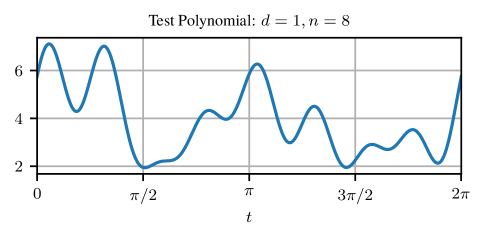
(a)

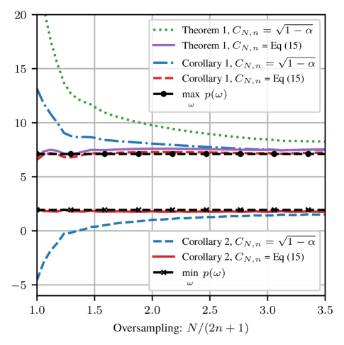
(b)

Figure 3: Example of upper and lower bounds for $p\in\bar{T}^{1}_{8}$ given by 50. (a): Test Polynomial. (b): Upper and lower bounds as a function of oversampling rate.

V-B Trivariate Example

For simplicity, we take $p\in\bar{T}_{n}^{3}$ to be the Dirichlet kernel of (uniform) degree $n$; that is, $p(\omega)=D_{n}^{3}(\omega)$ given by 21.

We obtain uniform samples of $p(\omega)$ over $\Theta^{d}_{N}$ by computing a zero-padded Discrete Fourier Transform. In particular, we embed an $n\times n\times n$ array of ones into an $N\times N\times N$ array of zeros, and apply the Fast Fourier Transform algorithm to this array. We choose $N$ to be a favorable size for the FFT algorithm, such as a power of two. As we choose $N$ proportional to the degree $n$ of $p$, our method scales as $\mathcal{O}(n^{d}\log{n})$ with $d=3$ in this example.

Fig. 4 shows the estimates obtained using Corollaries 1 and 2 as a function of $N$ for a variety of orders $n$; the true maximum value of $p(\omega)$ is $1$ and the minimum can be shown to be roughly $-2/(3\pi)\approx-0.22$. Evaluating the bounds for $n=32$ and $N=512$ took roughly one second on a workstation with an Intel i7-6700K CPU and $32$GB of RAM.

To draw a comparison with the sum-of-squares framework, we use the POS3POLY MATLAB library, in particular the function min_poly_value_multi_general_trig_3_5 [24]. This function finds the minimum value of a polynomial (given its coefficients) by a solving an SDP feasibility problem using an interior point method; the maximum value is obtained by calling the same function on $-p$. The per-iteration complexity of this method is $\mathcal{O}(n^{4d})$.

For $n=7$, POS3POLY required $75$ seconds to obtain the minimum value to within $3\times 10^{-3}$; $n=8$ required $260$ seconds and found the minimum to within of $2\times 10^{-3}$. The $n=9$ case exhausted the system memory and was too large to solved on the workstation.

This is meant to be an illustrative, but certainly not exhaustive, comparison between the bounds presented in this paper and the sum-of-squares framework. Sum-of-squares methods are especially attractive if an exact solution is needed or if the polynomial has sparse coefficients, in which case the complexity can be dramatically reduced.

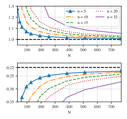
Figure 4: Upper and lower bounds for the Dirichlet kernel of 3 variables using Corollaries 1 and 2 as a function of number of samples, $N$.

VI Application to 2D Filter Bank Design

VI-A Perfect Reconstruction Filter Banks

We review a few key properties of multirate perfect reconstruction filter banks before turning to our design algorithm; see [25, 8] for a complete overview.

An $N_{c}$ channel analysis filter bank operating on $d$-dimensional signals consists of a collection of $N_{c}$ analysis filters $h_{i}$ and a non-singular downsampling matrix $M\in\mathbb{Z}^{d\times d}$. A filter bank is perfect reconstruction (PR) if there exists a (possibly non-unique) synthesis filter bank, consisting of a collection of $N_{c}$ synthesis filters, $g_{i}$, and the upsampling matrix $M$, that reconstructs a signal from its analyzed version. An analysis filter bank, along with its corresponding synthesis filter bank, are illustrated in Fig. 5. If the filter bank is PR then $\hat{x}=x$. In what follows, a ’filter bank’ indicates an analysis filter bank unless otherwise specified.

Figure 5: An $N_{c}$ channel multi-rate filter bank with analysis filters $h_{i}$ and synthesis filters $g_{i}$.

We consider finite impulse response (FIR) filters, and for simplicity, we restrict our attention to impulse responses with a square support. A real (square) $d$-variate (or $d$-dimensional) FIR filter $h$ of length $n$ is a function $h:\mathbb{Z}^{d}\to\mathbb{R}$ such that $h[m]=0$ if $m_{i}<0$ or $m_{i}\geq n$ for any $0\leq i<d$.

A multidimensional discrete-time signal is a function $x:\mathbb{Z}^{d}\to\mathbb{R}$. Downsampling a signal $x$ by a non-singular integer matrix $M$ retains only the samples on the lattice generated by $M$; that is, integer vectors of the form $v=Mt$. The simplest choice of downsampling matrix is $M=sI_{d}$, where the integer $s\geq 1$ controls the downsampling factor and $I_{d}$ is the identity matrix in $d$ dimensions. We will refer to this as the uniform downsampling scheme.

The $i$-th polyphase component of a signal $x$ is a function $\hat{x}^{i}:\mathbb{Z}^{d}\to\mathbb{R}$ obtained by shifting and downsampling $x$. In particular, $\hat{x}^{i}[m]=x[Mm+v_{i}]$ for $m\in\mathbb{Z}^{d}$, where $v_{i}$ is an integer vector of the form $Mt$ and $t\in[0,1)^{d}$. There are $\left|M\right|\triangleq\det{M}$ such integer vectors, and each generates one polyphase component of the signal. The $z$-transform of the $i$-th polyphase component of $x$ is $\hat{X}^{i}(z)=\sum_{n\in\mathbb{Z}^{d}}x[Mn+v_{i}]z^{-n}$, where $z\in\mathbb{C}^{d}$ and $z^{-n}=z_{1}^{-n_{1}}z_{2}^{-n_{2}}\ldots z_{d}^{-n_{d}}$.

The polyphase decomposition of an analysis filter is defined in a similar fashion. The $i$-th polyphase component of the analysis filter $h$ is $\hat{h}^{k}[m]=h[Mm-v_{i}]$; note the difference in sign when compared to the definition of $\hat{x}^{i}$.

A $d$-dimensional filter bank with filters $\left\{h_{i}\right\}_{i=1}^{N_{c}}$ and downsampling matrix $M$ has a polyphase matrix $\hat{\mathbf{H}}(z)\in\mathbb{C}^{N_{c}\times\left|M\right|}$ formed by stacking the polyphase components of each analysis filter into a row vector, and stacking the $N_{c}$ rows into a matrix. Explicitly,

$$\hat{\mathbf{H}}(z)\triangleq\begin{bmatrix}\hat{H}_{0}^{0}(z)&\hat{H}_{0}^{1}(z)&\ldots&\hat{H}_{0}^{\left|M\right|-1}(z)\\ \hat{H}_{1}^{0}(z)&\hat{H}_{1}^{1}(z)&\ldots&\hat{H}_{1}^{\left|M\right|-1}(z)\\ \vdots&\vdots&\ddots&\vdots\\ \hat{H}_{N^{c}-1}^{0}(z)&\hat{H}_{N^{c}-1}^{1}(z)&\ldots&\hat{H}_{N_{c}-1}^{\left|M\right|-1}(z)\\ \end{bmatrix},$$ (51)

where $\hat{H}^{k}_{i}(z)$ is the $z$-transform of the $k$-th polyphase component of the $i$-th filter. The entries of $\hat{\mathbf{H}}(z)$ are multi-variate Laurent polynomials in $z\in\mathbb{C}^{d}$ and become trigonometric polynomials when restricted to the unit circle; that is, $z=e^{j\omega}$ with $\omega\in\mathbb{T}^{d}$. In a customary abuse of notation, we write $\hat{\mathbf{H}}(\omega)\triangleq\hat{\mathbf{H}}(e^{j\omega})$.

There are deep connections between perfect reconstruction filter banks and redundant signal expansions using frames [12, 26, 27, 28]. In particular, oversampled perfect reconstruction filter banks implement an frame expansion. Associated with a perfect reconstruction filter bank are a pair of scalars, the upper and lower frame bounds, defined by

$$A \triangleq\mathrm{ess\ sup}_{\omega\in\mathbb{T}^{d},m=1,\ldots\left|M\right|}\ \lambda_{n}(\omega),$$ (52)

$$B \triangleq\mathrm{ess\ inf}_{\omega\in\mathbb{T}^{d},m=1,\ldots\left|M\right|}\ \lambda_{n}(\omega)$$ (53)

where $\lambda_{n}(\omega)$ is an eigenvalue of the matrix $\hat{\mathbf{H}^{*}}(\omega)\hat{\mathbf{H}}(\omega)$. If $A=B$ the frame is said to be tight. The ratio $A/B$ is the frame condition number; if $A/B\approx 1$, the frame is said to be well-conditioned. The frame bounds of a filter bank determine important numerical properties such as sensitivity to perturbations, and the frame condition number serves a similar role as the condition number of a matrix.

The synthesis filter bank also admits a polyphase decomposition. The $i$-th polyphase component of a synthesis filter $g$ is $\hat{g}^{k}[m]=g[Mm+v_{i}]$. The synthesis polyphase matrix is of size $\left|M\right|\times N_{c}$ and has entries

$$\hat{\mathbf{G}}(z)\triangleq\begin{bmatrix}\hat{G}_{0}^{0}(z)&\hat{G}_{1}^{0}(z)&\ldots&\hat{G}_{\left|M\right|-1}^{0}(z)\\ \hat{G}_{0}^{1}(z)&\hat{G}_{1}^{1}(z)&\ldots&\hat{G}_{\left|M\right|-1}^{1}(z)\\ \vdots&\vdots&\ddots&\vdots\\ \hat{G}_{0}^{N^{c}-1}(z)&\hat{G}_{1}^{N^{c}-1}(z)&\ldots&\hat{G}_{\left|M\right|-1}^{N_{c}-1}(z)\\ \end{bmatrix}.$$ (54)

If a pair of analysis and synthesis filter banks share the PR property, then $\hat{\mathbf{G}}(z)\hat{\mathbf{H}}(z)=I_{\left|M\right|}$, where $I_{\left|M\right|}$ is the $\left|M\right|\times\left|M\right|$ identity matrix. That is, $\hat{\mathbf{G}}(z)$ is a left inverse for $\hat{\mathbf{H}}(z)$. If $N_{c}>\left|M\right|$, the filter bank is said to be oversampled, and the synthesis filter bank is not unique. A particular choice is the minimum-norm synthesis filter bank, given by

$$\hat{\mathbf{H}}^{\dagger}(z)\triangleq\left(\tilde{\mathbf{H}}(z)\hat{\mathbf{H}}(z)\right)^{-1}\tilde{\mathbf{H}}(z),$$ (55)

where the para-conjugate matrix $\tilde{\mathbf{H}}(z)$ is obtained by conjugating the polynomial coefficients of $\hat{\mathbf{H}}(z)$, replacing the argument $z$ by $z^{-1}$, and transposing the matrix. On the unit circle, $\hat{\mathbf{H}}^{\dagger}(\omega)=\left(\hat{\mathbf{H}}^{*}(\omega)\hat{\mathbf{H}}(\omega)\right)^{-1}\hat{\mathbf{H}}^{*}(\omega)$.

A filter bank is perfect reconstruction if and only if its polyphase matrix has full column rank on the unit circle [6, 12]. As the matrix $\hat{\mathbf{H}}^{*}(\omega)\hat{\mathbf{H}}(\omega)$ is positive semidefinite, the perfect reconstruction property holds if and only if the trigonometric polynomial

$$p_{H}(\omega)\triangleq\det\left(\hat{\mathbf{H}}^{*}(\omega)\hat{\mathbf{H}}(\omega)\right)$$ (56)

is strictly positive. This property is key to our proposed filter bank design algorithm.

The degree of $p_{H}(\omega)$ depends on the filter length and the downsampling matrix. To illustrate, we bound from above the degree of $p_{H}(\omega)$ when using separable downsampling. After downsampling by $M=sI_{d}$, a FIR filter of length $n$ retains at most $\mathrm{ceil}(n/s)$ entries along each dimension; thus the polyphase component $\hat{H}_{i}^{k}(\omega)$ has maximum component degree $n^{\prime}\triangleq\mathrm{ceil}(n/s)-1$. Note that $\hat{H}_{i}^{k}(\omega)$ contains only negative powers of $\omega$; that is, $\hat{H}_{i}^{k}(\omega)\in\mathrm{span}\left\{e^{-jk\cdot\omega}:\omega\in\mathbb{T}^{d},k\in\mathbb{Z}^{d},\ n^{\prime}\leq k_{i}\leq 0\right\}$. As such, the trigonometric polynomials $(\hat{H}^{k}_{i}(\omega))^{*}\hat{H}^{l}_{i}(\omega)$ remain in $T_{n^{\prime}}^{d}$ and the entries of the matrix $\hat{\mathbf{H}}^{*}(\omega)\hat{\mathbf{H}}(\omega)$ are in the same space.

At worst, the determinant includes the product of $\left|M\right|=s^{d}$ polynomials of degree $n^{\prime}$, and so $p_{H}\in\bar{T}^{d}_{m}$ with

$$m\leq s^{d}(\mathrm{ceil}(n/s)-1).$$ (57)

Taking $n=12,s=2$ and $d=2$, we have $p_{H}\in T^{2}_{20}$.

VI-B Filter Bank Design: Analysis

The simplest multi-dimensional PR filter banks apply a 1D PR filter bank independently to each signal dimension; for example, in 2D, to the horizontal and vertical directions. These separable filters are written as a product of multiple 1D filters and suffer from limited directional sensitivity. The design and construction of non-separable multi-dimensional filter banks is difficult due to the lack of a spectral factorization theorem [9]; indeed, directly verifying the perfect reconstruction condition for a 2D filter bank is equivalent to determining the minimum value of a trigonometric polynomial and is thus NP-Hard [3, 4].

Some 2D PR filter banks, such as curvelets, have been hand-designed [29, 30]. Other design methods include variable transformations applied to a 1D PR filter bank [25, 8], modulating a prototype filter [25], invoking tools from algebraic geometry [10], or by solving an optimization problem [31, 32].

Optimizing a filter bank subject to the PR condition is a semi-infinite optimization problem: we have a finite number of design variables, namely the filter coefficients, and the resulting polyphase matrix must be positive semidefinite over $\mathbb{T}^{d}$.

One approach is to carefully parameterize the filter bank architecture in such a way that guarantees the PR property [9, 32]. A different approach is to relax the PR condition to near PR, and minimize the resulting reconstruction error using an iterative algorithm [31].

We use a different approach: we relax the semi-infinite problem into a finite one, then use Corollary 3 to certify that the solution of the relaxed problem is also a solution to the original problem. In particular, we design the filter bank such that $p_{H}(\omega)$ is strictly positive over the finite collection of sampling points $\Theta_{N}^{d}$. Corollary 3 tells us that if the bounds 19 or 20 are satisfied, then $p_{H}(\omega)$ is strictly positive over all of $\mathbb{T}^{d}$, and the filter bank is thus PR.

We design our filter banks with an eye towards the bounds of Corollary 3: we want the maximum and minimum sampled values of $p_{H}(\omega)$ to be close to one another, so that the bounds 19 and 20 are satisfied for smaller values of $N$.

Our filter design approach is highly flexible. It applies to arbitrary filter lengths, any non-singular decimation matrix, and will design PR filter banks in any number of dimensions. For simplicity we focus on designing real, 2D filter banks ($d=2$) but our approach can be modified for $d$-dimensional complex filters.

We begin by specifying the number of channels, $N_{c}$, downsampling matrix $M$, and filter size. We require that $N_{c}\geq\left|M\right|$ so that the PR condition can hold. For simplicity, we use downsampling of the form $M=sI_{2}$, but our method can design filter banks using non-separable (e.g., quincunx) downsampling matrices. We also constrain each filter to be of size $n\times n$, although this can be easily relaxed.

With these parameters set, we calculate the maximum degree $m$ of $p_{H}(\omega)$ using 57. Next, we select the number of sampling points, $N$, to use during the design process. The conditions of Corollary 3 require we take $N\geq 2m+1$, but in practice we take $N>4m$ so that we can tolerate larger values of $\kappa_{N}$ while still certifying the perfect reconstruction property.

The $i$-th $n\times n$ filter will be written $h_{i}$, and we group the filters into a tensor $H\in\mathbb{R}^{N_{c}\times n\times n}$. The Discrete-Time Fourier Transform of the $i$-th filter is

$$h_{i}(\omega)=\sum_{m\in[n]^{2}}h_{i}[m]e^{j\omega\cdot m}\quad\omega\in\mathbb{T}^{2},$$ (58)

and the squared magnitude response of $h_{i}$ is $\left|h_{i}(\omega)\right|^{2}$.

Our goal is to design a perfect reconstruction filter bank where the magnitude response of the $i$-th channel matches a desired real and non-negative magnitude response $D_{i}(\omega)$ for $\omega\in\mathbb{T}^{2}$. We use a weighted quadratic penalty that measures the discrepancy between the magnitude response of a candidate filter and the $D_{i}$ at the 2D-DFT samples $\Theta^{2}_{N}$. Our filter design function is written

$$f(H,D)\triangleq\sum_{i=1}^{N_{c}}\sum_{\omega\in\Theta^{2}_{N}}W_{i}(\omega)\cdot\left|\left|\hat{h}_{i}(\omega)\right|^{2}-D_{i}(\omega)\right|^{2},$$ (59)

where we have introduced weighting functions $W_{i}(\omega)$ to control the importance given to the passband, transition band, and stop band. If $D_{i}$ is not specified for some $i$, we take $W_{i}(\omega)$ to be uniformly zero; then $h_{i}$ does not contribute to $f(H,D)$ but may contribute to the PR property of the filter bank.

We emphasize that other choices of a design function are possible; for instance, one could use a minimax criterion and minimize the maximum deviation between $\hat{h}_{i}(\omega)$ and $D_{i}(\omega)$. Elsewhere, we have used a similar approach to learn signal-adapted undecimated perfect reconstruction (analysis) filter banks under a sparsity-inducing criterion [33].

In some cases, the filter design function alone may promote perfect reconstruction filter banks- for instance, when designing a non-decimated $(M=I_{d})$ filter bank where the desired magnitude responses satisfy a partition-of-unity condition. In general, though, this term is not enough. We add an additional regularization term to encourage filter banks that can be certified as perfect reconstruction using Corollary 3. Our regularizer is given by

$$R(H)\triangleq\alpha\sum_{i=1}^{N_{c}}\lVert h_{i}\rVert_{F}^{2}+\sum_{\omega\in\Theta^{2}_{N}}\beta p_{H}(\omega)^{2}-\gamma\log{p_{H}(\omega)},$$ (60)

where the non-negative scalars $\alpha,\beta,\gamma$ are tuning parameters. The first term prohibits the filter norms from becoming too large. The second and third terms apply the function $\omega\mapsto p_{H}(\omega)^{2}-\log{p_{H}(\omega)}$ for each $\omega\in\Theta^{2}_{N}$. The negative logarithm barrier function becomes large when $p_{H}(\omega)$ goes to zero and the quadratic part discourages large values of $p_{H}(\omega)$.

Together, these terms ensure the matrix $\hat{\mathbf{H}}(\omega)$ is left invertible and well-conditioned for each $\omega\in\Theta^{2}_{N}$. They also ensure $p_{H}(\omega)$ does not grow too large over the sampling set. These properties ensure $p_{H}(\omega)$ is strictly positive and doesn’t vary too much over $\Theta^{2}_{N}$; thus, by Corollary 3, $R(H)$ promotes well-conditioned perfect reconstruction filter banks. We emphasize that this regularizer, as well as the filter design function, are only computed over on the discrete set $\Theta^{2}_{N}$; passage to the continuous case is handled by Corollary 3.

Our designed filter bank is the solution to the optimization problem

$$\min_{H\in\mathcal{C}}f(H,D)+R(H),$$ (61)

where the constraint set $\mathcal{C}$ reflects any additional constraints on the filters, e.g. symmetry.

This minimization can be solved using standard first order methods such as gradient descent. The main challenge is calculating the gradient of $\log(p_{H}(\omega))$, which is unwieldy for all but the shortest filters. A finite-difference approximation to the gradient can suffice, but we have had success using the reverse-mode automatic differentiation capabilities of the autograd and Pytorch Python packages. Our algorithm is implemented in Pytorch and runs on an NVidia Titan X GPU.

VI-C Experiment: Design of a curvelet-like filter bank

Our goal is to design a filter bank that approximates the discrete curvelet filter bank. Our desired magnitude responses are obtained from the frequency space tiling illustrated in Fig. 6; each channel should have a pass-band corresponding to a cell in this tiling. As the magnitude frequency response of a real filter is symmetric, e.g. $\left|\hat{h}(\omega_{1},\omega_{2})\right|=\left|\hat{h}(-\omega_{1},-\omega_{2})\right|$, $17$ filters are needed for the desired partitioning. We use uniform downsampling by a factor of $2$, that is, $M=2I_{2}$. The filter bank is roughly $4\times$ oversampled.

The weighting functions $W_{i}(\omega)$ were set to $1$. We set $\beta=10$ and $\alpha=\gamma=1$. We used $5000$ iterations of the Adam optimization algorithm with a learning rate of $10^{-2}$ [34]. The optimization completed in under one minute for all tasks.

We designed two filter banks; one with $8\times 8$ filters and the other with $11\times 11$ filters. We used $N=64$ for both cases. The final filter banks and their magnitude responses are shown in Fig. 7.

We tested two methods to initialize the algorithm. In the first method, we take an $N\times N$ inverse DFT of the desired magnitude response, $D_{i}$, and extract the $n\times n$ central region of the resulting impulse response. Our second method is a simple random initialization. Both methods perform equally well in our design task.

We use Corollary 3 to verify the final filter banks are perfect reconstruction. For our filter bank with $8\times 8$ filters, the bound 57 indicates $p_{H}\in\bar{T}^{2}_{12}$. Our sufficient condition in Corollary 3 for strict positivity requires $\kappa_{64}\leq 4.4$, with $\kappa_{N}$ given by 19. We computed $p_{H}(\omega)$ over all points in $\Theta_{64}^{2}$, and used these values to compute $\kappa_{64}$. We found $\kappa_{64}=1.3$ for the designed filter bank, and thus the filter bank is perfect reconstruction. When using $11\times 11$ filters, we have $p_{H}\in\bar{T}^{2}_{20}$. This filter bank too is perfect reconstruction, as $\kappa_{64}=1.8\leq 2.2$.

Figure 6: Desired tiling of frequency space.

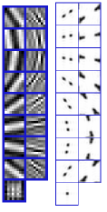
(a)

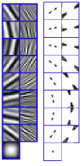
(b)

Figure 7: Optimized 17 channel filter bank. The left column of each subfigure shows the filter impulse response. The right column shows the magnitude frequency response, with $\omega=0$ located at the center of each blue box. (a) 17 channel filter bank with $8\times 8$ filters. (b) 17 channel filter bank with $11\times 11$ filters.

VI-D Filter Bank Design: Synthesis

Our filter design problem has focused exclusively on the analysis portion of the filter bank, but in many applications the synthesis filter bank is equally important.

We focus on the oversampled case, i.e. $N_{c}>\left|M\right|$. The choice of synthesis filter bank is not unique. We have already seen one possible choice- the minimum-norm synthesis filter bank 55, which can be obtained explicitly once the analysis filter bank has been designed. In general, the minimum-norm synthesis filter bank consists of infinite impulse response (IIR) filters [35, 12].

In many applications, IIR filters are not practical- only FIR filters can be used, and short FIR filters are especially desirable from a computational perspective.

Fortunately, the redundancy of an oversampled filter bank affords us design flexibility. Sharif investigated when a generic one-dimensional oversampled PR analysis filter bank admits a synthesis filter bank with short FIR filters. He found that almost all sufficiently oversampled PR analysis filter banks have such a synthesis filter bank, and obtained bounds on the minimum synthesis filter length [36]. The bounds depend only on the number of channels, downsampling factor, and analysis filter length, but not on the filter coefficients themselves.

We have a few options if a FIR synthesis filter bank is desired. The simplest solution is to truncate the (IIR) minimum-norm synthesis filters to a particular length. Indeed, a well-conditioned PR analysis filter bank has minimum-norm synthesis filters with coefficients that exhibit decay exponentially with filter length, implying that the minimum-norm synthesis filter bank can be well-approximated by FIR filters [37].

A second option is to use tools from algebraic geometry to find an FIR synthesis filter bank, if one exists [38].

We adopt a third option: we incorporate the desire for an FIR synthesis filter bank directly into the design problem. We add an additional set of FIR filters, denoted $\left\{g_{i}\right\}_{i=1}^{N_{c}}$, to the design parameters. The synthesis filters need not be the same length as the analysis filters. Our goal is for the polyphase matrix associated with the synthesis filter bank, $\hat{\mathbf{G}}(\omega)$, to be a left inverse of the analysis polyphase matrix. This condition is represented by the constraint

$$\hat{\mathbf{G}}(\omega)\hat{\mathbf{H}}(\omega)=I_{\left|M\right|}.$$ (62)

In practice, we solve an unconstrained problem using the quadratic penalty method: we penalize the distance between $\hat{\mathbf{G}}(\omega)\hat{\mathbf{H}}(\omega)$ and $I_{\left|M\right|}$ for each $\omega\in\Theta_{N}^{2}$ using the Frobenius norm [39]. Our modified design problem is given by

$$\min_{H,G\in\mathcal{C}}f(H,D)+R(H)+\lambda\sum_{\omega\in\Theta_{N}^{2}}\lVert\hat{\mathbf{G}}(\omega)\hat{\mathbf{H}}(\omega)-I_{\left|M\right|}\rVert_{F}^{2}.$$ (63)

We again use a first order method, but now increase $\lambda$ as a function of the iteration number so as to ensure $\hat{\mathbf{G}}(\omega)$ is a left inverse of $\hat{\mathbf{H}}(\omega)$.

As before, our new regularizer is evaluated only over $\Theta_{N}^{2}$, not $\mathbb{T}^{2}$. For fixed, finite filter lengths, the entries of $\hat{\mathbf{G}}(\omega)\hat{\mathbf{H}}(\omega)$ are real trigonometric polynomials of bounded degree, and we can use the bounds of Corollaries 1 and 2 to either ensure the constraint 62 holds over $\mathbb{T}^{2}$ or to estimate and bound the amount that the constraint has been violated.

VI-E Experiment: Filter Bank Design with FIR Synthesis Filters

We repeat the design experiment from Section VI-C using the new objective function 63. As before, we use 17 channels and take $M=2I_{2}$, leading to a roughly $4\times$ oversampled filter bank. We work with $11\times 11$ filters. We used $5000$ iterations of the Adam optimization algorithm with a learning rate of $10^{-2}$, and set the parameter $\lambda:=\log_{2}(i)$ at iteration $i$.

Fig. 8 collects the design results. Fig. 8a shows the $11\times 11$ analysis filters embedded into a larger $40\times 40$ region. This is done to facilitate comparison with the minimum-norm synthesis filters, shown in Fig. 8b. The minimum-norm synthesis filters exhibit fast decay, as expected for a well-conditioned filter bank. The designed FIR synthesis filters, the $\left\{g_{i}\right\}_{i=1}^{N_{c}}$, are shown in Fig. 8c. These filters have no discernible structure. However, we computed $\lVert\hat{\mathbf{G}}(\omega)\hat{\mathbf{H}}(\omega)-I_{\left|M\right|}\rVert_{F}^{2}<10^{-7}$ for each $\omega\in\Theta_{128}^{2}$, this is a synthesis filter bank for $\hat{\mathbf{H}}$. Indeed, passing the standard barbara test image through the pair of analysis and synthesis filter banks yielded a reconstruction peak signal to noise ratio (PSNR) of more than $80$ dB.

Fig. 9 illustrates the coefficient decay properties of the minimum-norm synthesis filters. We show the square root of the absolute value of the filter coefficients to compress the dynamic range of the image. We see the expected exponential decay of filter coefficients associated with a well-conditioned filter bank[37].

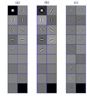
Figure 8: Analysis and Synthesis filters for filter bank designed in Section VI-E. (a) Designed $11\times 11$ analysis filters embedded into $40\times 40$ filter. (b) Minimum-norm synthesis filters, obtained using 55. The filters exhibit fast coefficient decay; see Fig. 9. (c) Designed $16\times 16$ FIR synthesis filters.

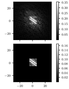
Figure 9: Square-root of absolute value of filter coefficients from one of the filters in Fig. 8a. Top: Minimum-norm synthesis filter exhibits fast coefficient decay, can be approximated with FIR filter. Bottom: FIR analysis filter.

VII Conclusion

We have proposed a fast and simple method to estimate the extremal values of a multivariate trigonometric polynomial directly from its samples. We have extended an existing upper bound from univariate to multivariate polynomials, and developed a strengthened upper bound and new lower bound for real trigonometric polynomials. The lower bound provides a new sufficient condition to certify global positivity of a real multivariate trigonometric polynomial, and this condition motivated a new method to design two-dimensional, multirate, perfect reconstruction filter banks. The demonstration of this application in this paper is a preliminary study for the proposed filter bank design algorithm; we plan to further investigate this design methodology, including extensions to non-uniform and/or data-adaptive filter banks.

References

- [1] K. Jetter, G. Pfander, and G. Zimmermann, “The crest factor for trigonometric polynomials. Part I: Approximation theoretical estimates,” Rev. Anal. Numér. Théor. Approx., vol. 30, pp. 179–195, 2001.
- [2] B. Dumitrescu, Positive Trigonometric Polynomials and Signal Processing Applications, ser. Signals and Communication Technology. Springer International Publishing, 2017.
- [3] K. G. Murty and S. N. Kabadi, “Some NP-complete problems in quadratic and nonlinear programming,” Mathematical Programming, vol. 39, pp. 117–129, 1987.
- [4] P. A. Parrilo, “Semidefinite programming relaxations for semialgebraic problems,” Mathematical Programming, vol. 96, pp. 293–320, 2003.
- [5] P. A. Parrilo and B. Sturmfels, “Minimizing polynomial functions,” DIMACS Series in Discrete Mathematics and Theoretical Computer Science, 2001.
- [6] M. Vetterli, “A theory of multirate filter banks,” IEEE Trans. Acoust., Speech, Signal Process., vol. 35, pp. 356–372, 1987.
- [7] P. Vaidyanathan, Multirate systems and filter banks. Prentice Hall, 1992.
- [8] M. N. Do, “Multidimensional filter banks and multiscale geometric representations,” FNT in Signal Processing, vol. 5, pp. 157–164, 2011.
- [9] S. Venkataraman and B. Levy, “State space representations of 2-D FIR lossless transfer matrices,” IEEE Trans. Circuits Syst. II, vol. 41, pp. 117–132, 1994.
- [10] J. Zhou, M. Do, and J. Kovacevic, “Multidimensional orthogonal filter bank characterization and design using the Cayley transform,” IEEE Trans. Image Process., vol. 14, pp. 760–769, 2005.
- [11] F. Delgosha and F. Fekri, “Results on the factorization of multidimensional matrices for paraunitary filterbanks over the complex field,” IEEE Trans. Signal Process., vol. 52, pp. 1289–1303, 2004.
- [12] Z. Cvetkovic and M. Vetterli, “Oversampled filter banks,” IEEE Trans. Signal Process., vol. 46, pp. 1245–1255, May 1998.
- [13] B. S. Albrecht Böttcher, Introduction to Large Truncated Toeplitz Matrices. Springer New York, 1999.
- [14] R. M. Gray, “Toeplitz and circulant matrices: A review,” Foundations and Trends in Communications and Information Theory, vol. 2, pp. 155–239, 2005.
- [15] T. F. Chan and J. A. Olkin, “Circulant preconditioners for Toeplitz-block matrices,” Numerical Algorithms, vol. 6, pp. 89–101, 1994.
- [16] R. H. Chan, J. G. Nagy, and R. J. Plemmons, “Circulant preconditioned Toeplitz least squares iterations,” SIAM Journal on Matrix Analysis and Applications, vol. 15, pp. 80–97, Jan. 1994.
- [17] V. F. Pisarenko, “The retrieval of harmonics from a covariance function,” Geophysical Journal International, vol. 33, pp. 347–366, 1973.
- [18] T. Laudadio, N. Mastronardi, and M. V. Barel, “Computing a lower bound of the smallest eigenvalue of a symmetric positive-definite toeplitz matrix,” IEEE Trans. Inf. Theory, vol. 54, pp. 4726–4731, 2008.
- [19] A. Zygmund, Trigonometric series. Cambridge University Press, 2005.
- [20] T. Sørevik and M. A. Nome, “Trigonometric interpolation on lattice grids,” BIT Numerical Mathematics, vol. 56, pp. 341–356, 2015.
- [21] G. Wunder and H. Boche, “Peak magnitude of oversampled trigonometric polynomials,” Frequenz, vol. 56, pp. 102–109, 2002.
- [22] J. G. Proakis and D. K. Manolakis, Digital Signal Processing, 4th ed. Prentice Hall, 2006.
- [23] R. S. Elias M. Stein, Fourier analysis: an introduction. Princeton University Press, 2003.
- [24] B. Şicleru and B. Dumitrescu, “POS3POLY—a MATLAB preprocessor for optimization with positive polynomials,” Optim. Eng., vol. 14, pp. 251–273, 2013.
- [25] Y.-P. Lin and P. P. Vaidyanathan, “Theory and design of two-dimensional filter banks: A review,” Multidimensional Systems and Signal Processing, vol. 7, pp. 263–330, 1996.
- [26] H. Bolcskei, F. Hlawatsch, and H. Feichtinger, “Frame-theoretic analysis of oversampled filter banks,” IEEE Trans. Signal Process., vol. 46, pp. 3256–3268, 1998.
- [27] O. Christensen, An introduction to frames and Riesz bases. Birkhäuser, 2003.
- [28] G. Strang and T. Nguyen, Wavelets and Filter Banks. Wellesley College, 1996.
- [29] E. J. Candes and D. L. Donoho, “New tight frames of curvelets and optimal representations of objects with piecewise singularities,” Commun. Pure Appl. Math., vol. 57, pp. 219–266, 2004.
- [30] E. Candès, L. Demanet, D. Donoho, and L. Ying, “Fast discrete curvelet transforms,” Multiscale Modeling & Simulation, vol. 5, pp. 861–899, 2006.
- [31] W.-S. Lu, A. Antoniou, and H. Xu, “A direct method for the design of 2-D nonseparable filter banks,” IEEE Transactions on Circuits and Systems II: Analog and Digital Signal Processing, vol. 45, pp. 1146–1150, 1998.
- [32] Y. Chen, M. D. Adams, and W.-S. Lu, “Design of optimal quincunx filter banks for image coding via sequential quadratic programming,” in 2007 IEEE International Conference on Acoustics, Speech and Signal Processing - ICASSP ’07, - 2007, p. nil.
- [33] L. Pfister and Y. Bresler, “Learning filter bank sparsifying transforms,” 2018,” arXiv:1803.01980 [stat.ML].
- [34] D. P. Kingma and J. Ba, “Adam: A method for stochastic optimization,” CoRR, 2014, arXiv:1412.6980 [cs.LG].
- [35] H. Bolcskei, “A necessary and sufficient condition for dual weyl-heisenberg frames to be compactly supported,” The Journal of Fourier Analysis and Applications, vol. 5, pp. 409–419, 1999.
- [36] B. Sharif and Y. Bresler, “Generic feasibility of perfect reconstruction with short FIR filters in multichannel systems,” IEEE Transactions on Signal Processing, vol. 59, pp. 5814–5829, 2011.
- [37] T. Strohmer, Finite-and Infinite-Dimensional Models for Oversampled Filter Banks. Boston, MA: Birkhäuser Boston, 2001, pp. 293–315.
- [38] J. Zhou and M. N. Do, “Multidimensional oversampled filter banks,” in Wavelets XI, 8 2005.
- [39] J. N. S. J. Wright, Numerical optimization. Springer, 2006.