Inclusive prompt photon production in electron-nucleus scattering at small $x$

Abstract

We compute the differential cross-section for inclusive prompt photon production in deeply inelastic scattering (DIS) of electrons on nuclei at small $x$ in the framework of the Color Glass Condensate (CGC) effective theory. The leading order (LO) computation in this framework resums leading logarithms in $x$ as well as power corrections to all orders in $Q_{s,A}^{2}/Q^{2}$, where $Q_{s,A}(x)$ is the nuclear saturation scale. This LO result is proportional to universal dipole and quadrupole Wilson line correlators in the nucleus. In the soft photon limit, the Low-Burnett-Kroll theorem allows us to recover existing results on inclusive DIS dijet production. The $k_{\perp}$ and collinearly factorized expressions for prompt photon production in DIS are also recovered in a leading twist approximation to our result. In the latter case, our result corresponds to the dominant next-to-leading order (NLO) perturbative QCD contribution at small $x$. We next discuss the computation of the NLO corrections to inclusive prompt photon production in the CGC framework. In particular, we emphasize the advantages for higher order computations in inclusive photon production, and for fully inclusive DIS, arising from the simple momentum space structure of the dressed quark and gluon “shock wave” propagators in the “wrong” light cone gauge $A^{-}=0$ for a nucleus moving with $P^{+}_{N}\rightarrow\infty$.

I Introduction

The measurement of isolated prompt photons in deeply inelastic scattering (DIS) provides a unique precision test of perturbative QCD (pQCD) with two distinct hard scales that are well understood from QED: the exchanged photon virtuality, $Q^{2}$ in the initial state and the transverse energy of the emitted prompt photon, $E_{\perp}^{\gamma}$. Prompt photon cross-sections were measured early on by the H1 and ZEUS experiments Breitweg et al. (2000); Aktas et al. (2005); Chekanov et al. (2007) for the case of photoproduction, where the negative 4-momentum transfer squared, $Q^{2}=-q^{2}$ of the exchanged virtual photon is close to zero. Subsequently, the first measurements of prompt photon production in $e+p$ DIS, isolated and accompanied by jets, were performed by ZEUS and H1 for a wide range of $Q^{2}$ Chekanov et al. (2004); Aaron et al. (2008); Chekanov et al. (2010); Abramowicz et al. (2012).

Isolated photons in DIS have proven to be clean and well calibrated probes of QCD dynamics Gehrmann-De Ridder et al. (2006); Schmidt et al. (2016). We will explore here their potential for uncovering a novel gluon saturation regime of QCD Gribov et al. (1983); Mueller and Qiu (1986) at small Bjorken $x$. This regime is characterized by the many-body recombination and screening dynamics of gluons that competes with the perturbative bremsstrahlung of increasing numbers of soft gluons at small $x$. An emergent dynamical scale $Q_{s,A}(x)$ screens color charges at increasingly smaller distances with decreasing $x$ thereby ensuring that the squared field strengths do not exceed $1/\alpha_{S}$, where $\alpha_{S}$ is the QCD coupling constant. The dynamics in this regime of QCD is fully nonlinear. Nevertheless, at sufficiently small $x$, or large enough nuclear size $A$, where $Q_{s,A}^{2}(x)\gg\Lambda_{\rm QCD}^{2}$, $\alpha_{S}\equiv\alpha_{S}(Q_{s,A})\ll 1$. Many-body weak coupling techniques can therefore be employed to perform systematic computations in this nonlinear QCD regime McLerran and Venugopalan (1994a, b, c).

The rich dynamics of gluon saturation is captured in an effective field theory (EFT), the Color Glass Condensate (CGC) McLerran and Venugopalan (1994a, b, c); Iancu and Venugopalan (2003); Gelis et al. (2010); Kovchegov and Levin (2012); Blaizot (2017), and we will apply it here to compute the inclusive photon cross-section in DIS off nuclei. The CGC EFT is formulated in the infinite momentum frame Fubini and Furlan (1965); Bardakci and Halpern (1968); Weinberg (1966); Susskind (1968) of the nucleus with an appropriate choice of gauge. It relies on the separation, in the longitudinal momentum fraction $x$, of the degrees of freedom into static color sources at large $x$ coupled eikonally to dynamical “wee” gluon fields at small $x$ Gelis et al. (2010). Because a large number of large $x$ sources couple to the wee gluons, the color charge of the sources can lie in any one of a number of higher dimensional color representations of the $SU(3)$ algebra McLerran and Venugopalan (1994a); Jeon and Venugopalan (2004). This results in a stochastic distribution of classical color sources over a gauge invariant weight functional $W_{Y_{A}}[\rho_{A}]$ representing the probability density of the color charge density $\rho_{A}(x^{-},\mathbf{x}_{\perp})$. The subscript $Y_{A}=\text{ln}(x_{0}/x)$ denotes the spacetime rapidity separation of small $x$ target gluons relative to those at $x\equiv x_{0}$ corresponding to the nuclear beam rapidity, $Y_{beam}$.

The expectation value of any physical operator at rapidity $Y_{A}$ is determined by the average over all possible color charge configurations:

$$\left\langle\mathcal{O}\right\rangle_{Y_{A}}=\int[\mathcal{D}\rho_{A}]\enskip W_{Y_{A}}[\rho_{A}]\mathcal{O}[\rho_{A}]\enskip,$$ (1)

where $\mathcal{O}[\rho_{A}]$ is the expectation value of the operator for a particular configuration $\rho_{A}$ of color sources. In the problem of interest, this operator is the differential cross-section for inclusive photon production for a given $\rho_{A}$. Requiring that physical observables be independent of the arbitrary scale separation between sources and fields results in the JIMWLK functional renormalization group equation Jalilian-Marian et al. (1997, 1998); Iancu et al. (2001a, b); Ferreiro et al. (2002)

$$\frac{\partial W_{Y_{A}}[\rho_{A}]}{\partial Y_{A}}=\mathcal{H}\big{[}\rho_{A},\frac{\delta}{\delta\rho_{A}}\big{]}\enskip W_{Y_{A}}[\rho_{A}]\enskip.$$ (2)

This equation describes the evolution of the distribution of color charges in the nuclear wavefunction from its fragmentation region at large $x$ (or small $Y_{A}$) to the small $x$ (or large $Y_{A}$) of interest as determined by the kinematics of the process. Here $\mathcal{H}$ is the JIMWLK Hamiltonian; explicit expressions and properties of the Hamiltonian are discussed for instance in Iancu and Venugopalan (2003); Weigert (2005). It is worthwhile to note here that the JIMWLK evolution equation can alternatively be expressed as the Balitsky-JIMWLK hierarchy Balitsky (1996); Weigert (2002) of equations for expectation values of $n$-point Wilson line correlators. In the limit of large number of colors $N_{c}\rightarrow\infty$ and for large nuclei $A\rightarrow\infty$, the closed form Balitsky-Kovchegov (BK) equation is obtained for the two-point correlator of Wilson lines Balitsky (1996); Kovchegov (1999). The BK equation is a good approximation in many practical situations to the full Balitsky-JIMWLK hierarchy Rummukainen and Weigert (2004); Dumitru et al. (2011) and is therefore extremely useful in phenomenological studies at collider experiments.

An attractive feature of the CGC, as in any EFT, is that there is a well defined power counting for systematic higher order computations. As we will show explicitly later for our specific case, this power counting allows one to match results in the CGC framework to those in the collinear factorization and $k_{\perp}$ factorization perturbative frameworks in appropriate kinematic limits. For $e+A$ and $p+A$ collisions, the appropriate CGC power counting is in a so-called “dilute-dense” limit Gelis et al. (2010) where dilute color source density $\rho_{p}$ in the generic projectile is of order $g\ll 1$ in the QCD coupling, while the density of color sources $\rho_{A}\sim 1/g$ in the nuclear target. Strictly speaking, the dilute-dense power counting corresponds to computations that are lowest order in the dimensionless ratios $Q_{s,p}^{2}/k_{p,\perp}^{2}\ll 1$, and all orders in $Q_{s,A}^{2}/k_{A,\perp}^{2}\sim 1$, where $k_{p,\perp}$ and $k_{A,\perp}$ correspond to the momentum transfer from the projectile and target respectively. The dilute-dense power counting was implemented recently by one of us and collaborators in computing inclusive photon production in $p+A$ collisions to next-to-leading order (NLO) accuracy Benic et al. (2017) extending earlier leading order (LO) computations in this context Gelis and Jalilian-Marian (2002).

The power counting in the CGC framework for the $e+A$ DIS case at hand is simpler than the $p+A$ case because we don’t have a power counting in $\rho_{p}$ on account of the lepton probe. In general, at LO in the QCD coupling constant, we obtain the two classes of processes shown in Fig. 1 that contribute to the inclusive prompt photon cross-section.

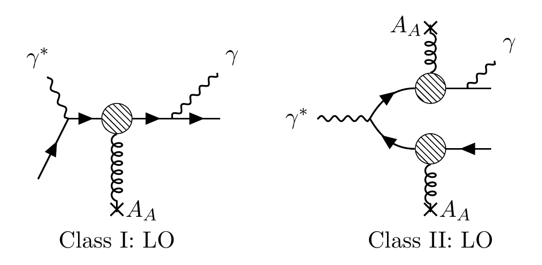
Figure 1: Representative diagrams for leading order (LO) processes contributing to inclusive prompt photon production in DIS. For Class II processes, the photon can be emitted from either fermion line. The blobs represent the resummed eikonal interactions between the quark/antiquark and the classical color field of the nucleus.

The Class I processes represent the bremsstrahlung of a photon from a valence quark in the wavefunction of the target nucleus. Their contribution to the differential cross-section for inclusive photon production has been calculated Gelis and Jalilian-Marian (2002); Dominguez et al. (2011) at small $x$ in the CGC framework albeit in the context of $p+A$ collisions. This result can however be straightforwardly adapted to the present problem.

The Class II processes correspond to configurations that become important at small $x$ where the virtual photon emitted by the electron fluctuates into a long lived quark-antiquark dipole Gribov et al. (1966); Ioffe (1969) and the dipole subsequently has a nearly instantaneous “shock wave” eikonal scattering off the gauge fields in the nuclear target Bjorken et al. (1971); Nikolaev and Zakharov (1991); Kovchegov and Levin (2012). In this dipole picture of $e+A$ DIS, the power counting is dictated by strong color sources $\rho_{A}\sim 1/g$ in the target, and their energy evolution with respect to the quark-antiquark dipole. Attaching new sources to the diagram in Fig. 1 does not change the order in strong coupling constant, because $g\rho_{A}\sim 1$. Independent powers of $g$ arise only when a vertex is not connected to the source. From this argument, it should be clear that we are performing an all-twist expansion in $g\rho_{A}$ at each order in $\alpha_{S}$ in this power counting scheme.

At NLO, typical contributions to Class I processes are shown in Fig. 2. For inclusive photon production, these possess the divergence structure inherent in NLO quark production containing i) dominant contributions from the large phase space in transverse momentum available to the emitted gluon ($\alpha_{S}\text{ln}(k_{\perp})\sim 1$), ii) subdominant contribution from logarithms sensitive to $x$ (since valence quark distributions are peaked at $x\sim 1$) and finally, iii) finite pieces that are not phase space enhanced. By an appropriate choice of scale and scheme for factorization, the finite pieces can be absorbed in the definition of the quark distribution function. These contributions are therefore effectively of order $\mathcal{O}(\alpha_{e})$ (where $\alpha_{e}$ is the QED fine structure constant) if we replace the bare valence quark distribution in the nucleus by one that absorbs the leading logarithmic contributions. These last contributions, to all orders in perturbation theory, are captured by the DGLAP Dokshitzer (1977); Gribov and Lipatov (1972); Altarelli and Parisi (1977) renormalization group (RG) evolution of the valence quark distributions.

At small $x$, the Class I contributions are strongly suppressed relative to the Class II contribution. The reason for this is that the former are sensitive to the valence quark distribution in the target while the latter are sensitive to the gluon distribution. At small $x$, as seen in the $e+p$ HERA DIS data Abe et al. (1993); Ahmed et al. (1995); Derrick et al. (1993, 1995); Martin et al. (1994); Lai et al. (1995), the gluon distribution clearly dominates the valence quark distribution. Since our interest is in inclusive photon production at small $x$, we shall not examine Class I type processes any further and shall focus our attention exclusively on Class II processes.

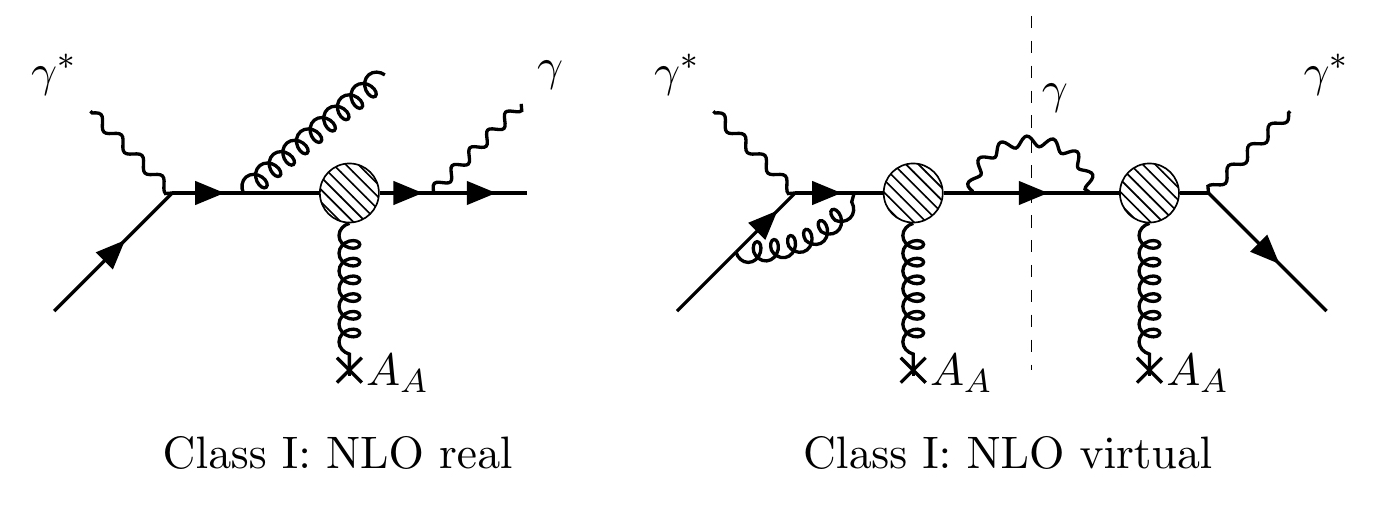
Figure 2: Representative diagrams for the Class I processes that contribute at NLO to inclusive photon production. Both real emission and interference contributions are shown.

In the first part of this paper, we will compute the Class II LO diagrams shown in Fig. 1. We will subsequently discuss the structure of the NLO computation of inclusive photon production. We shall in particular discuss a simple formulation of the dressed gluon propagator in light cone gauge. The NLO computations are important for two reasons. Firstly, as noted in our discussion of Class I NLO contributions, there are logarithmically enhanced contributions of order $\alpha_{S}\ln(x_{0}/x)$ which can be as large as the LO contributions. Such contributions appear in each order of perturbation theory; they can be isolated and resummed in a so-called leading logarithmic (LLx) RG treatment. There are also pure $\alpha_{S}$ suppressed NLO contributions. These are important for precision measurements but can also lead to qualitative changes in spectra that impact the discovery potential of such measurements. In particular, they will be important for a quantitative extraction of the saturation scale $Q_{s,A}(x)$.

These statements can be understood more clearly by considering the organization of the perturbative series for the argument of $\langle\mathcal{O}\rangle$ in Eq. 1 as

$$\mathcal{O}[\rho_{A}]=\sum_{n=0}c_{n}\alpha_{S}^{n}\enskip.$$ (3)

Here each coefficient $c_{n}=\sum_{j=1}^{\infty}\xi_{nj}(g\rho_{A})^{j}$, where the matrix elements $\xi_{nj}$ are numbers of order unity, resums the contributions obtained by adding extra sources of magnitude $\rho_{A}\sim 1/g$ to the allowed graphs. Before we proceed any further, we must invoke the essential ingredient of the CGC effective field theory – the separation of large $x$ static light cone sources from dynamical small $x$ gauge fields – as represented by the structure of Eq. 1.

The starting point of any CGC computation therefore includes an initial cutoff scale $\Lambda_{0}^{+}$ (in the $`+$’ longitudinal momentum) or $Y_{0}$ (in the rapidity) between sources and fields. This is shown schematically in Fig. 3. At leading order (LO), the cutoff scale $\Lambda_{0}^{+}$ (or $Y_{0}=\ln(\Lambda_{\rm beam}/\Lambda_{0}^{+})$) distinguishing soft and hard partons is arbitrary and the fast quantum modes with $k^{+}\gg\Lambda^{+}_{0}$ or $Y<Y_{0}$ are represented by the classical color source density $\rho_{A}$ with the weight functional $W_{\Lambda_{0}^{+}(Y_{0})}[\rho_{A}]$. The quantum evolution of sources and fields is described by the following renormalization group procedure (RG). One first integrates out quantum fluctuations within the range $\Lambda_{1}^{+}<|k^{+}|<\Lambda_{0}^{+}$. Here $\Lambda_{1}^{+}$ is chosen such that $\alpha_{S}\ln(\Lambda_{0}^{+}/\Lambda_{1}^{+})\equiv\alpha_{S}\Delta Y<1$, where $\Delta Y=Y_{1}-Y_{0}$.

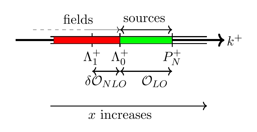
Figure 3: Schematic illustration of sources and fields in the CGC effective theory in terms of the cutoff scale $\Lambda_{0}^{+}$ and equivalently rapidity, $Y_{0}$. At LO, this separation is arbitrary. At NLO, contribution from field modes in the range $\Lambda_{1}^{+}<k^{+}<\Lambda_{0}^{+}$, such that $\alpha_{S}\ln(\Lambda_{0}^{+}/\Lambda_{1}^{+})\equiv\alpha_{S}\Delta Y<1$, are integrated out and absorbed into the source densities at the scale $\Lambda_{1}^{+}$. This self-similar renormalization group (RG) pattern is repeated successively generating the JIMWLK RG equation for the source densities. See text for a detailed discussion.

For our computation of inclusive photon production at small $x$, typical NLO diagrams that generate such logarithms upon change of scale from $\Lambda_{0}^{+}$ to $\Lambda_{1}^{+}$ are shown in Fig. 4. Their contribution can be absorbed into the evolution of the weight functional describing the distribution of color sources:

$$W_{\Lambda_{1}^{+}}[\rho_{A}] =\Big{(}1+\text{ln}(\Lambda_{0}^{+}/\Lambda_{1}^{+}).\mathcal{H}\Big{)}W_{\Lambda_{0}^{+}}[\rho_{A}]\quad\text{or equivalently,}$$

$$W_{Y_{1}}[\rho_{A}] =\Big{(}1+\Delta Y.\mathcal{H}\Big{)}W_{Y_{0}}[\rho_{A}]\enskip.$$ (4)

Here $\mathcal{H}$ is the JIMWLK Hamiltonian we alluded to previously. Hence these particular NLO $\delta\mathcal{O}$ contributions generate a classical effective theory at this new scale expressed as

$$\int[\mathcal{D}\rho_{A}]\enskip W_{\Lambda_{0}^{+}}[\rho_{A}](\mathcal{O}_{LO}+\delta\mathcal{O}_{NLO})=\int[\mathcal{D}\rho_{A}]\enskip W_{\Lambda_{1}^{+}}[\rho_{A}]\mathcal{O}[\rho_{A}]\enskip,$$ (5)

where the LLx contributions have been absorbed in the JIMWLK evolution of $W$. To leading order accuracy, the perturbative expansion in Eq. 3 then has the coefficients:

$$c_{n}=\sum_{j=0}^{\infty}d_{nj}(g\rho_{A})^{j}\Big{(}\text{ln}(1/x)\Big{)}^{n},\qquad n=1,2,\ldots\enskip,$$ (6)

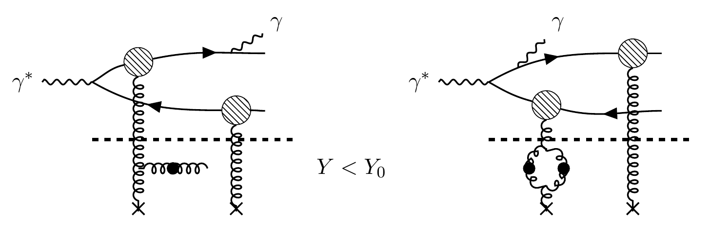
Figure 4: Representative Feynman graphs contributing at NLO to the evolution of color sources. In the CGC effective theory, the integration over gluon field modes with rapidity $Y<Y_{0}$ is given by contributions from these classes. These contributions are actually $O(1)$ in magnitude because of the presence of large logarithms in $x$ leading to $\alpha_{S}\text{ln}(1/x)\sim 1$.

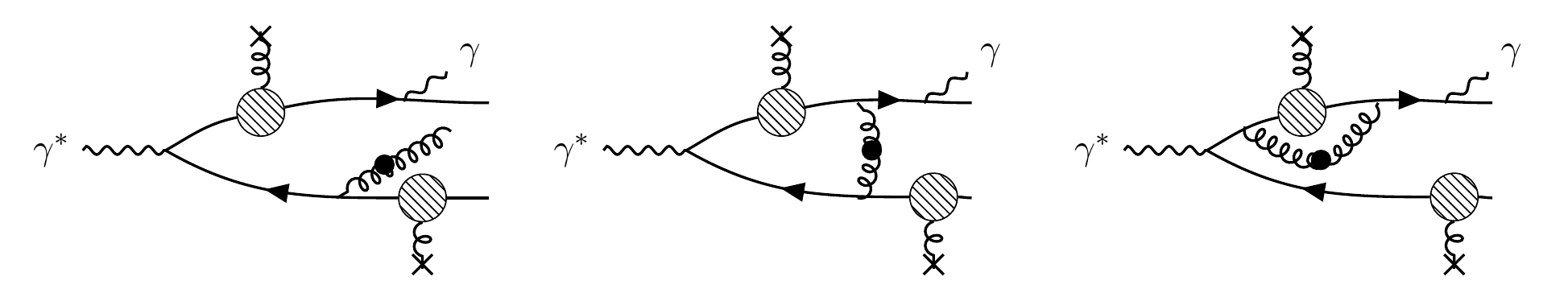
Figure 5: Some of the Feynman graphs contributing at NLO to inclusive photon production in $e+A$ DIS at small $x$. These generate O($\alpha_{S}$) corrections to inclusive photon production.

At NLO however, there are $\alpha_{S}$ contributions that do not come accompanied with logarithms in $x$. These would then correspond to coefficients expressed more generally in the expansion of the perturbative series as

$$c_{n}=\sum_{i=0}^{n}\sum_{j=0}^{\infty}f_{nj}^{i}(g\rho_{A})^{j}\Big{(}\text{ln}(1/x)\Big{)}^{i},\qquad n=1,2,\ldots\enskip,$$ (7)

in particular the coefficients $f_{nj}^{n-1}$. For our process of interest, some of the the corresponding diagrams are shown in Fig. 5. These additional contributions are not rapidity ordered relative to the leading order contribution; the phase space integrals therefore do not generate logarithms in $x$. Thus while the NLO diagrams represented in Fig. 4 can be absorbed into the LO order computation of photon production accompanied by leading logarithmic JIMWLK evolution of the weight functional $W$, the NLO graphs represented in Fig. 5 should be combined with next-to-leading-log (NLLx) JIMWLK evolution to obtain the full NLO result for inclusive photon production in $e+A$ collisions at small $x$. Fortunately, the NLLx JIMWLK evolution equations are known Balitsky and Chirilli (2013); Grabovsky (2013); Kovner et al. (2014) as well as the NLLx BK equations Kovchegov and Weigert (2007); Balitsky and Chirilli (2008); Balitsky (2007). Therefore with the computation of the NLO diagrams represented in Fig. 5, all the elements will be in place for quantitative predictions, to NLO accuracy, for inclusive photon production in $e+A$ collisions at small $x$. This paper represents the first step in this direction. While we will discuss key aspects of the structure of the NLO computation here, the full computation will be presented in future publications in preparation.

The paper is organized as follows. In section II, we begin by discussing the ingredients necessary for the computation of the amplitude for inclusive photon production; a compact expression for this amplitude is given in Eq. 47. In section III, we will calculate the cross-section for the production of a direct photon accompanied by a quark-antiquark pair as well as the inclusive differential cross-section for direct photon production at LO. The former provides the rate for inclusive production of a photon with a dijet pair in small $x$ kinematics. Our results for these cross-sections are expressed respectively in Eqs. 58 and 59 as a convolution of the lepton tensor $L^{\mu\nu}$ that is familiar from inclusive DIS and a hadron tensor constituted of all-twist lightlike Wilson line correlators. In section IV, which we divide into three subsections, we discuss the important properties of the photon production amplitude at leading order. We first examine the $k_{\perp}$ and collinear factorization limits of our computation in the limit of large transverse momentum $k_{\perp}\gg Q^{A}_{S}$. In the former case, the cross-section is proportional to the unintegrated gluon distribution within the nucleus while the latter is proportional to the usual leading twist nuclear gluon distribution in perturbative QCD, evaluated at the scale $Q^{2}$ of the virtual photon. The corresponding expressions for the hadron tensor in this limit are given in Eqs. 63 and 76 respectively. We next demonstrate that the Low-Burnett-Kroll theorem Low (1958); Burnett and Kroll (1968); Bell and Van Royen (1969) is satisfied when $k_{\gamma}\rightarrow 0$: we see explicitly that the nonradiative DIS differential cross-section for the inclusive dijet case in DIS matches extant results in the literature for the same Dominguez et al. (2011). In the final subsection, we show that the amplitude derived in Eq. 47 has a simple and efficient interpretation in terms of a modified fermion propagator in the classical background field of the nucleus. This will prove beneficial for higher order computations.

Section V outlines the machinery for the computation of the amplitude at NLO. This includes a discussion of the motivation behind choosing the “wrong” light cone gauge $A^{-}=0$ for the kinematics of our process as the efficient gauge in which to perform our computations. We then derive the corresponding momentum space Feynman rules for the small fluctuation gluon propagator and conclude this section with an analysis of the contributing processes at this order. We end the paper with a brief summary and an outline of work in progress.

Appendices A, B and C supplement the material in the body of the paper. The notations and conventions are clarified in Appendix A. Appendix B includes the proof of gauge invariance by virtue of the Ward identity. It also contains computational detail for the subsection dealing with the soft photon factorization of the photon production amplitude. Appendix C includes a detailed discussion of the techniques used in determining kinematically allowed processes contributing to inclusive photon production at both LO and NLO.

II Components of the LO amplitude computation

In this section, we will outline the components needed for the computation of the amplitude for Class II processes at LO in the CGC framework. In the effective theory of CGC, owing to their large occupancy $A\sim 1/g$, the dynamics of small $x$ gluons to LO is described by the classical Yang-Mills equations

$$[D_{\mu},F^{\mu\nu}](x)=g\delta^{\nu+}\delta(x^{-})\rho_{A}(\mathbf{x}_{\perp})\enskip.$$ (8)

The nucleus is assumed to move in the positive $z$-direction at nearly the speed of light with large light cone longitudinal momentum $P^{+}_{N}\rightarrow\infty$. (See Appendix A for the conventions adopted in this work.) We also assume in this frame that the virtual photon has a large $q^{-}$ component of its momentum.

An essential element in the computation of the LO amplitude is the fermion propagator in the background strong classical color field of the nucleus. In Lorenz gauge $\partial_{\mu}A^{\mu}=0$, this has the coordinate space representation McLerran and Venugopalan (1999)

$$S_{A}(x,y)=S_{0}(x,y)+\bigg{[}\theta(x^{-})\theta(-y^{-})\int\mathrm{d}^{4}z\enskip\delta(z^{-})\big{(}\tilde{U}(\mathbf{z}_{\perp})-1\big{)}-\theta(-x^{-})\theta(y^{-}) \int\mathrm{d}^{4}z\enskip\delta(z^{-})\big{(}\tilde{U}^{\dagger}(\mathbf{z}_{\perp})-1\big{)}\bigg{]}$$

$$\times S_{0}(x,z)\gamma^{-}S_{0}(z,y)\enskip,$$ (9)

where

$$S_{0}(x,y)=\int\frac{\mathrm{d}^{4}p}{(2\pi)^{4}}e^{-ip.(x-y)}S_{0}(p),\quad S_{0}(p)=\frac{i(\not{p}+m)}{p^{2}-m^{2}+i\varepsilon}\enskip,$$ (10)

is the free fermion propagator.

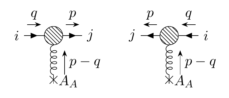
Figure 6: Effective vertices for the quark and antiquark respectively. Here $i$ and $j$ represent color indices in the fundamental representation.

This effective propagator appears in the momentum space Feynman rules as an effective vertex with the following factors,

$$\mathcal{T}_{ji}(q,p)=\pm(2\pi)\delta(p^{-}-q^{-})\gamma^{-}\int\mathrm{d}^{2}\mathbf{x}_{\perp}\enskip e^{i(\mathbf{q}_{\perp}-\mathbf{p}_{\perp}).\mathbf{x}_{\perp}}\big{[}\tilde{U}^{(\pm)}(\mathbf{x}_{\perp})-1\big{]}_{ji}\enskip,$$ (11)

where the plus (minus) sign corresponds to insertions on a quark (antiquark) line respectively and the Wilson line $\tilde{U}$ is written in the fundamental representation of $SU(N_{c})$ as

$$\tilde{U}(\mathbf{x_{\perp}})=\mathcal{P}_{-}\text{exp}\left[-ig^{2}\int_{-\infty}^{+\infty}\mathrm{d}z^{-}\frac{1}{\nabla^{2}_{\perp}}\rho_{A}^{a}(z^{-},\mathbf{x_{\perp}})t^{a}\right].$$ (12)

In Feynman diagrams, this effective vertex insertion is drawn as depicted in Fig. 6. These effective vertices do not change the order of the diagrams parametrically by any power of $g$. In principle therefore there can be diagrams with multiple insertions with the emitted photon sandwiched between any two such vertices. However there is a kinematic constraint that restricts many such possibilities: On the same fermion line(quark or antiquark), there cannot be a photon sandwiched between two effective vertices. This has the physical meaning that an outgoing fermion (with a definite sign of $p^{-}$) can get scattered off of the nucleus and subsequently emit a photon but does not suffer a secondary scattering because the time scale governing the scattering is of order $1/P^{+}_{N}$, which is nearly instantaneous in the infinite momentum frame.

II.1 Derivation of the amplitude

The amplitude for the process

$$e(\tilde{l})+A(P)\rightarrow e(\tilde{l^{\prime}})+Q(k)+\overline{Q}(p)+\gamma(k_{\gamma})+X\enskip,$$ (13)

with $X$ denoting any other particle produced in the collision, can be written as

$$\mathcal{M}(\mathbf{\tilde{l}},\mathbf{\tilde{l^{\prime}}},\mathbf{q},\mathbf{k},\mathbf{p},\mathbf{k}_{\gamma})=\frac{e}{Q^{2}}\overline{u}(\tilde{l^{\prime}})\gamma^{\mu}u(\tilde{l})\mathcal{M}_{\mu}(\mathbf{q},\mathbf{k},\mathbf{p},\mathbf{k}_{\gamma};\lambda)\enskip,$$ (14)

where

$$\mathcal{M}_{\mu}(\mathbf{q},\mathbf{k},\mathbf{p},\mathbf{k}_{\gamma};\lambda)=\epsilon^{*\alpha}(\mathbf{k}_{\gamma},\lambda)\mathcal{M}_{\mu\alpha}(\mathbf{q},\mathbf{k},\mathbf{p},\mathbf{k}_{\gamma})\enskip,$$ (15)

represents the amplitude for the hadronic subprocess and is the quantity of interest. Here $\epsilon^{\alpha}(\mathbf{k}_{\gamma},\lambda)$ is the polarization vector for the outgoing photon. The momentum assignments are summarized in Table 1 and boldface letters stand for the corresponding 3-momenta. Squaring the expression for the amplitude in Eq. 14, and performing the necessary averaging and sum over electron spins, we can write

$$\frac{1}{2}\sum_{\text{spins},\lambda}|\mathcal{M}|^{2}=L^{\mu\nu}X_{\mu\nu}\enskip.$$ (16)

Here

$$L^{\mu\nu}=\frac{2e^{2}}{Q^{4}}\Big{[}(\tilde{l}^{\mu}\tilde{l}^{\prime\nu}+\tilde{l}^{\nu}\tilde{l}^{\prime\mu})-\frac{Q^{2}}{2}g^{\mu\nu}\Big{]}\enskip,$$ (17)

is the lepton tensor that is identical to that obtained in inclusive DIS. The hadron tensor

$$X_{\mu\nu}=-\sum_{\text{spins}}\mathcal{M}_{\mu\alpha}^{*}(\mathbf{q},\mathbf{k},\mathbf{p},\mathbf{k}_{\gamma}){\mathcal{M}_{\nu}}^{\alpha}(\mathbf{q},\mathbf{k},\mathbf{p},\mathbf{k}_{\gamma})\enskip,$$ (18)

is of course different because it allows for the emission of a photon from the quark-antiquark pair. After these bare preliminaries, we shall proceed to compute $\mathcal{M}_{\mu\alpha}$.

Table 1: 4-momentum assignments used in the calculation

$\tilde{l}$: Incoming electron	${\tilde{l}}^{\prime}$: Outgoing electron	$q$: Exchanged virtual photon
$k$: Quark, directed outward	$p$: Antiquark, directed outward	$k_{\gamma}$: Outgoing photon
$l$: Nucleus to antiquark line for multiple insertions
$P$: Total momentum of final state = $p+k+k_{\gamma}$

II.2 Classifying contributions to the amplitude

There are a total of ten contributions, which we will group into diagrams with gluon field insertions on the quark or antiquark line or both. The diagrams for the first group are shown in Fig. 7.

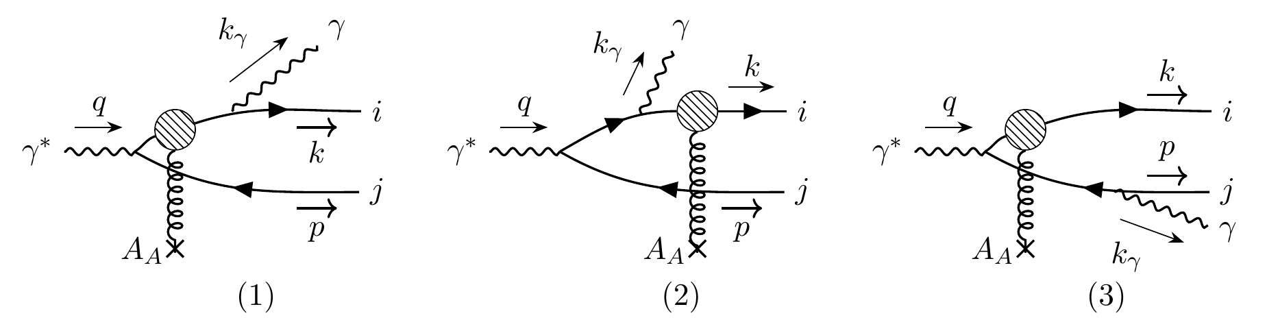
Figure 7: Contributions to the amplitude with one Wilson line insertion on the quark line. The momentum labels and their directions are clearly shown. $i$ and $j$ stand for color indices in the fundamental representation of $SU(N_{c})$.

The contribution to the amplitude from the diagram labeled (1), representing the emission of the photon by the quark subsequent to its multiple scatterings with the nucleus, is given by

$$\mathcal{M}^{(1)}_{\mu\alpha}(\mathbf{q},\mathbf{k},\mathbf{p},\mathbf{k}_{\gamma})=-(eq_{f})^{2}\enskip\overline{u}(\mathbf{k})\gamma_{\alpha}S_{0}(k+k_{\gamma})\mathcal{T}_{ij}(q-p,k+k_{\gamma})S_{0}(q-p)\gamma_{\mu}v(\mathbf{p})\enskip,$$ (19)

where $q_{f}$ is the charge of a quark/antiquark of a given flavor. Employing Eqs. 10 and 11, and choosing a frame where $\mathbf{q}_{\perp}=0$ for the virtual photon, we can write the above expression as

$$\mathcal{M}^{(1)}_{\mu\alpha}(\mathbf{q},\mathbf{k},\mathbf{p},\mathbf{k}_{\gamma})=2\pi(eq_{f})^{2}\delta(P^{-}-q^{-})\int_{\mathbf{x}_{\perp}}e^{-i\mathbf{P}_{\perp}.\mathbf{x}_{\perp}}\enskip\overline{u}(\mathbf{k})R^{(1)}_{\mu\alpha}(\mathbf{P}_{\perp})\Big{[}\tilde{U}(\mathbf{x}_{\perp})-1\Big{]}_{ij}v(\mathbf{p})\enskip,$$ (20)

where $\int_{\mathbf{x}_{\perp}}$ is a shorthand notation for $\int\mathrm{d}^{2}\mathbf{x}_{\perp}$, $i$ ($j$) represent the color indices of the quark (antiquark) respectively and

$$R^{(1)}_{\mu\alpha}(\mathbf{P}_{\perp}) =\gamma_{\alpha}\frac{(\not{k}+\not{k}_{\gamma}+m)}{(k+k_{\gamma})^{2}-m^{2}+i\varepsilon}\gamma^{-}\frac{\not{q}-\not{p}+m}{(q-p)^{2}-m^{2}+i\varepsilon}\gamma_{\mu}$$

$$=\frac{\gamma_{\alpha}\not{k}_{\gamma}+2k_{\alpha}}{(k+k_{\gamma})^{2}-m^{2}+i\varepsilon}\gamma^{-}\frac{\not{q}\gamma_{\mu}-2p_{\mu}}{(q-p)^{2}-m^{2}+i\varepsilon}\enskip.$$ (21)

We use the following relations

$$(\not{p}-m)\gamma_{\mu}v(\mathbf{p}) =2p_{\mu}v(\mathbf{p})\enskip,$$

$$\overline{u}(\mathbf{k})\gamma_{\alpha}(\not{k}+m) =2k_{\alpha}\overline{u}(\mathbf{k})\enskip,$$ (22)

to obtain the second line of Eq. 21. Note that the $\mathbf{P}_{\perp}$-dependence appearing in $R_{\mu\alpha}^{(1)}$ includes an implicit dependence on the three transverse momenta constituting $\mathbf{P}_{\perp}=\mathbf{k}_{\perp}+\mathbf{k}_{\gamma\perp}+\mathbf{p}_{\perp}$.

The contributions from diagrams (2) and (3) in Fig. 7 can be computed similarly; the sum of the contributions from these three diagrams can then be written as

$$\sum_{\beta=1}^{3}\mathcal{M}^{(\beta)}_{\mu\alpha}(\mathbf{q},\mathbf{k},\mathbf{p},\mathbf{k}_{\gamma})=2\pi(eq_{f})^{2}\delta(P^{-}-q^{-})\int_{\mathbf{x}_{\perp}}e^{-i\mathbf{P}_{\perp}.\mathbf{x}_{\perp}}\enskip\overline{u}(\mathbf{k})T^{(q)}_{\mu\alpha}(\mathbf{P}_{\perp})\Big{[}\tilde{U}(\mathbf{x}_{\perp})-1\Big{]}_{ij}v(\mathbf{p})\enskip,$$ (23)

where

$$T^{(q)}_{\mu\alpha}(\mathbf{P}_{\perp})=\sum_{\beta=1}^{3}R^{(\beta)}_{\mu\alpha}(\mathbf{P}_{\perp})\enskip,$$ (24)

with

$$R^{(2)}_{\mu\alpha}(\mathbf{P}_{\perp}) =\frac{\gamma^{-}(\not{q}-\not{P})+2k^{-}}{(q-p-k_{\gamma})^{2}-m^{2}+i\varepsilon}\gamma_{\alpha}\frac{\not{q}\gamma_{\mu}-2p_{\mu}}{(q-p)^{2}-m^{2}+i\varepsilon}\enskip,$$

$$R^{(3)}_{\mu\alpha}(\mathbf{P}_{\perp}) =-\frac{\gamma^{-}(\not{q}-\not{P})+2k^{-}}{(q-p-k_{\gamma})^{2}-m^{2}+i\varepsilon}\gamma_{\mu}\frac{\not{k}_{\gamma}\gamma_{\alpha}+2p_{\alpha}}{(p+k_{\gamma})^{2}-m^{2}+i\varepsilon}\enskip.$$ (25)

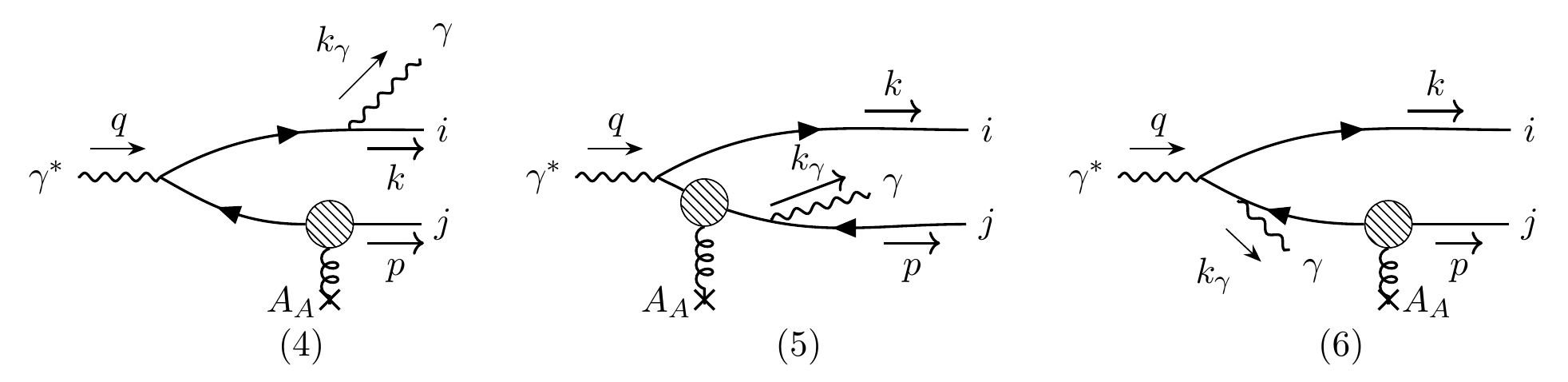
Figure 8: Contributions to the amplitude with one Wilson line insertion on the antiquark line. The momentum labels and their directions are clearly shown. $i$ and $j$ stand for color indices in the fundamental representation of $SU(N_{c})$.

Similarly, the contribution from diagrams with insertions on the antiquark line are shown in Fig. 8. Their collective contribution can be written as

$$\sum_{\beta=4}^{6}\mathcal{M}^{(\beta)}_{\mu\alpha}(\mathbf{q},\mathbf{k},\mathbf{p},\mathbf{k}_{\gamma})=2\pi(eq_{f})^{2}\delta(P^{-}-q^{-})\int_{\mathbf{y}_{\perp}}e^{-i\mathbf{P}_{\perp}.\mathbf{y}_{\perp}}\enskip\overline{u}(\mathbf{k})T^{(\bar{q})}_{\mu\alpha}(\mathbf{P}_{\perp})\Big{[}\tilde{U}^{\dagger}(\mathbf{y}_{\perp})-1\Big{]}_{ij}v(\mathbf{p})\enskip,$$ (26)

where

$$T^{(\bar{q})}_{\mu\alpha}(\mathbf{P}_{\perp})=\sum_{\beta=4}^{6}R^{(\beta)}_{\mu\alpha}(\mathbf{P}_{\perp})\enskip,$$ (27)

and

$$R^{(4)}_{\mu\alpha} (\mathbf{P}_{\perp})=\frac{\gamma_{\alpha}\not{k}_{\gamma}+2k_{\alpha}}{(k+k_{\gamma})^{2}-m^{2}+i\varepsilon}\gamma_{\mu}\frac{(\not{q}-\not{P})\gamma^{-}+2p^{-}}{(k+k_{\gamma}-q)^{2}-m^{2}+i\varepsilon}\enskip,$$

$$R^{(5)}_{\mu\alpha} (\mathbf{P}_{\perp})=\frac{2k_{\mu}-\gamma_{\mu}\not{q}}{(q-k)^{2}-m^{2}+i\varepsilon}\gamma^{-}\frac{\not{k}_{\gamma}\gamma_{\alpha}+2p_{\alpha}}{(p+k_{\gamma})^{2}-m^{2}+i\varepsilon}\enskip,$$

$$R^{(6)}_{\mu\alpha} (\mathbf{P}_{\perp})=\frac{2k_{\mu}-\gamma_{\mu}\not{q}}{(q-k)^{2}-m^{2}+i\varepsilon}\gamma_{\alpha}\frac{(\not{q}-\not{P})\gamma^{-}+2p^{-}}{(k+k_{\gamma}-q)^{2}-m^{2}+i\varepsilon}\enskip.$$ (28)

Finally, we need to consider the diagrams shown in Fig. 9 with insertions on both lines. For these cases, we will need to integrate over the nuclear momentum transfer $l$.

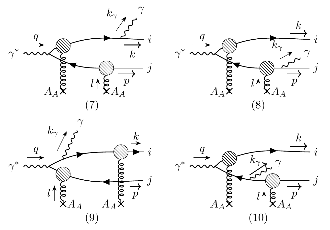
Figure 9: Contributions to the amplitude with two Wilson line insertions. The momentum labels and their directions are clearly shown. $i$ and $j$ stand for color indices in the fundamental representation of $SU(N_{c})$.

The contribution from the diagram labeled (7) can be written as

$$\mathcal{M}^{(7)}_{\mu\alpha}(\mathbf{q},\mathbf{k},\mathbf{p},\mathbf{k}_{\gamma})=-(eq_{f})^{2}\int\frac{\mathrm{d}^{4}l}{(2\pi)^{4}}\enskip\overline{u}(\mathbf{k})\gamma_{\alpha}S_{0}(k+k_{\gamma}) \mathcal{T}_{ik}(q-p+l,k+k_{\gamma})S_{0}(q-p+l)$$

$$\times\gamma_{\mu}S_{0}(l-p)\mathcal{T}_{kj}(-p,l-p)v(\mathbf{p})\enskip.$$ (29)

The integration over $l^{-}$ is trivial because of the $\delta(l^{-})$ factor from one of the effective vertices. The integration over $l^{+}$ can be done using the theorem of residues. The result can be again compactly written as

$$\mathcal{M}^{(7)}_{\mu\alpha}(\mathbf{q},\mathbf{k},\mathbf{p},\mathbf{k}_{\gamma})=2\pi(eq_{f})^{2}\delta(P^{-}-q^{-})\int_{\mathbf{x}_{\perp}}\int_{\mathbf{y}_{\perp}}\int_{\mathbf{l}_{\perp}}e^{-i\mathbf{P}_{\perp}.\mathbf{x}_{\perp}+i\mathbf{l}_{\perp}.\mathbf{x}_{\perp}} e^{-i\mathbf{l}_{\perp}.\mathbf{y}_{\perp}}\enskip\overline{u}(\mathbf{k})R^{(7)}_{\mu\alpha}(\mathbf{l}_{\perp},\mathbf{P}_{\perp})$$

$$\times\Big{[}\big{(}\tilde{U}(\mathbf{x}_{\perp})-1\big{)}\big{(}\tilde{U}^{\dagger}(\mathbf{y}_{\perp})-1\big{)}\Big{]}_{ij}v(\mathbf{p})\enskip,$$ (30)

where

$$R^{(7)}_{\mu\alpha}(\mathbf{l}_{\perp},\mathbf{P}_{\perp})=\frac{\gamma_{\alpha}\not{k}_{\gamma}+2k_{\alpha}}{(k+k_{\gamma})^{2}-m^{2}+i\varepsilon}\gamma^{-}\frac{\not{q}-\not{p}+\not{\mathbf{l}}_{\perp}+m}{N(\mathbf{l}_{\perp})}\gamma_{\mu}(\gamma^{-}\not{\mathbf{l}}_{\perp}+2p^{-})\enskip.$$ (31)

The factor

$$N(\mathbf{l}_{\perp})=4p^{-}(q^{-}-p^{-})\Big{[}q^{+}-\frac{M^{2}(\mathbf{l}_{\perp}-\mathbf{p}_{\perp})}{2p^{-}}-\frac{M^{2}(\mathbf{l}_{\perp}-\mathbf{p}_{\perp})}{2(q^{-}-p^{-})}\Big{]}\enskip,$$ (32)

appearing in the denominator is deliberately written in a way to make contact with the expression in Eq. 21; this will be exploited in a later part of the calculation. In the above, $M^{2}(\mathbf{p}_{\perp})=\mathbf{p}^{2}_{\perp}+m^{2}$ stands for the squared transverse mass and $\not{\mathbf{p}}_{\perp}=\gamma^{i}p_{i}$. Finally, $\int_{\mathbf{l}_{\perp}}$ is a shorthand notation for $\int\mathrm{d}^{2}\mathbf{l}_{\perp}/(2\pi)^{2}$.

The remaining three diagrams can be worked out similarly and and the combined result compactly written as

$$\sum_{\beta=7}^{10}\mathcal{M}^{(\beta)}_{\mu\alpha}(\mathbf{q},\mathbf{k},\mathbf{p},\mathbf{k}_{\gamma})=2\pi(eq_{f})^{2}\delta(P^{-}-q^{-}) \int_{\mathbf{x}_{\perp}}\int_{\mathbf{y}_{\perp}}\int_{\mathbf{l}_{\perp}}e^{-i\mathbf{P}_{\perp}.\mathbf{x}_{\perp}+i\mathbf{l}_{\perp}.\mathbf{x}_{\perp}}e^{-i\mathbf{l}_{\perp}.\mathbf{y}_{\perp}}$$

$$\times\overline{u}(\mathbf{k})T^{(q\bar{q})}_{\mu\alpha}(\mathbf{l}_{\perp},\mathbf{P}_{\perp})\Big{[}\big{(}\tilde{U}(\mathbf{x}_{\perp})-1\big{)}\big{(}\tilde{U}^{\dagger}(\mathbf{y}_{\perp})-1\big{)}\Big{]}_{ij}v(\mathbf{p})\enskip,$$ (33)

where

$$T^{(q\bar{q})}_{\mu\alpha}(\mathbf{l}_{\perp},\mathbf{P}_{\perp})=\sum_{\beta=7}^{10}R^{\beta}_{\mu\alpha}(\mathbf{l}_{\perp},\mathbf{P}_{\perp})\enskip.$$ (34)

The various R-factors obtained after the contour integration over $l^{+}$ are

$$R^{(8)}_{\mu\alpha}(\mathbf{l}_{\perp},\mathbf{P}_{\perp})=-\frac{\gamma^{-}(\not{q}-\not{P}+\not{\mathbf{l}}_{\perp})+2k^{-}}{(p+k_{\gamma})^{2}-m^{2}+i\varepsilon}\gamma_{\mu}(\not{p}+\not{k}_{\gamma}-\not{\mathbf{l}}_{\perp}-m)\gamma^{-}\frac{(\not{k}_{\gamma}\gamma_{\alpha}+2p_{\alpha})}{S(\mathbf{l}_{\perp})}\enskip,$$ (35)

$$R^{(9)}_{\mu\alpha}(\mathbf{l}_{\perp},\mathbf{P}_{\perp})=\Big{(}\gamma^{-}(\not{q}-\not{P}+\not{\mathbf{l}}_{\perp})+2k^{-}\Big{)}\gamma_{\alpha}(\not{q}-\not{p}+\not{l}_{a}+m)\gamma_{\mu}\frac{(\gamma^{-}\not{\mathbf{l}}_{\perp}+2p^{-})}{V(\mathbf{l}_{\perp})}\enskip,$$ (36)

and

$$R^{(10)}_{\mu\alpha}(\mathbf{l}_{\perp},\mathbf{P}_{\perp})=\Big{(}\gamma^{-}(\not{q}-\not{P}+\not{\mathbf{l}}_{\perp})+2k^{-}\Big{)}\gamma_{\mu}(\not{l}_{b}-\not{p}-\not{k}_{\gamma}+m)\gamma_{\alpha}\frac{(\gamma^{-}\not{\mathbf{l}}_{\perp}+2p^{-})}{W(\mathbf{l}_{\perp})}\enskip.$$ (37)

In the expressions above, the compactly written functions are

$$S(\mathbf{l}_{\perp})=4(p^{-}+k_{\gamma}^{-})(q^{-}-p^{-}-k_{\gamma}^{-})\Big{[}q^{+}-\frac{M^{2}(\mathbf{p}_{\perp}+\mathbf{k}_{\gamma\perp}-\mathbf{l}_{\perp})q^{-}}{2(p^{-}+k^{-}_{\gamma})(q^{-}-k^{-}_{\gamma}-p^{-})}\Big{]}\enskip,$$ (38)

$$V(\mathbf{l}_{\perp}) =8p^{-}(q^{-}-p^{-})(q^{-}-p^{-}-k^{-}_{\gamma})\Big{[}q^{+}-\frac{M^{2}(\mathbf{l}_{\perp}-\mathbf{p}_{\perp})q^{-}}{2p^{-}(q^{-}-p^{-})}\Big{]}$$

$$\times\Big{[}q^{+}-k^{+}_{\gamma}-\frac{M^{2}(\mathbf{l}_{\perp}-\mathbf{p}_{\perp})}{2p^{-}}-\frac{M^{2}(\mathbf{p}_{\perp}+\mathbf{k}_{\gamma\perp}-\mathbf{l}_{\perp})}{2(q^{-}-p^{-}-k^{-}_{\gamma})}\Big{]}\enskip,$$ (39)

and

$$W(\mathbf{l}_{\perp}) =8p^{-}(p^{-}+k^{-}_{\gamma})(q^{-}-p^{-}-k^{-}_{\gamma})\Big{[}q^{+}-\frac{M^{2}(\mathbf{p}_{\perp}+\mathbf{k}_{\gamma\perp}-\mathbf{l}_{\perp})q^{-}}{2(p^{-}+k^{-}_{\gamma})(q^{-}-p^{-}-k^{-}_{\gamma})}\Big{]}$$

$$\times\Big{[}q^{+}-k^{+}_{\gamma}-\frac{M^{2}(\mathbf{l}_{\perp}-\mathbf{p}_{\perp})}{2p^{-}}-\frac{M^{2}(\mathbf{p}_{\perp}+\mathbf{k}_{\gamma\perp}-\mathbf{l}_{\perp})}{2(q^{-}-p^{-}-k^{-}_{\gamma})}\Big{]}\enskip.$$ (40)

The factors $\not{l}_{a}$ and $\not{l}_{b}$ in Eqs. 36 and 37 are obtained by evaluating $\not{l}$ at the enclosed poles depending on the choice of contours:

$$\not{l}_{a} =\gamma^{-}\Bigg{(}p^{+}-\frac{M^{2}(\mathbf{l}_{\perp}-\mathbf{p}_{\perp})}{2p^{-}}\Bigg{)}+\not{\mathbf{l}}_{\perp}\enskip,$$

$$\not{l}_{b} =\gamma^{-}\Bigg{(}p^{+}+k^{+}_{\gamma}-q^{+}+\frac{M^{2}(\mathbf{p}_{\perp}-\mathbf{l}_{\perp}+\mathbf{k}_{\gamma\perp})}{2(q^{-}-p^{-}-k^{-}_{\gamma})}\Bigg{)}+\not{\mathbf{l}}_{\perp}\enskip.$$ (41)

II.3 Final expression for the amplitude

The net contribution from all the diagrams is obtained by adding the expressions in Eqs. 23, 26 and 33. Introducing a dummy integration $\int_{\mathbf{x}_{\perp}}\int_{\mathbf{k}_{\perp}}e^{-i\mathbf{k}_{\perp}.\mathbf{x}_{\perp}}=1$, this result can be expressed compactly as

$$\mathcal{M}_{\mu\alpha}(\mathbf{q},\mathbf{k},\mathbf{p},\mathbf{k}_{\gamma}) =\sum_{\beta=1}^{10}\mathcal{M}_{\mu\alpha}^{\beta}(\mathbf{q},\mathbf{k},\mathbf{p},\mathbf{k}_{\gamma})=2\pi(eq_{f})^{2}\delta(P^{-}-q^{-})\int_{\mathbf{x}_{\perp}}\int_{\mathbf{y}_{\perp}}\int_{\mathbf{l}_{\perp}}e^{-i\mathbf{P}_{\perp}.\mathbf{x}_{\perp}+i\mathbf{l}_{\perp}.\mathbf{x}_{\perp}}e^{-i\mathbf{l}_{\perp}.\mathbf{y}_{\perp}}$$

$$\times\overline{u}(\mathbf{k})\Big{[}T^{(q\bar{q})}_{\mu\alpha}(\mathbf{l}_{\perp},\mathbf{P}_{\perp})\big{[}\tilde{U}(\mathbf{x}_{\perp})\tilde{U}^{\dagger}(\mathbf{y}_{\perp})-1\big{]}+\Big{(}T^{(q)}_{\mu\alpha}(\mathbf{P}_{\perp})-T^{(q\bar{q})}_{\mu\alpha}(\mathbf{l}_{\perp},\mathbf{P}_{\perp})\Big{)}\big{[}\tilde{U}(\mathbf{x}_{\perp})-1\big{]}$$

$$+\Big{(}T^{(\bar{q})}_{\mu\alpha}(\mathbf{P}_{\perp})-T^{(q\bar{q})}_{\mu\alpha}(\mathbf{l}_{\perp},\mathbf{P}_{\perp})\Big{)}\big{[}\tilde{U}^{\dagger}(\mathbf{y}_{\perp})-1\big{]}\Big{]}v(\mathbf{p})\enskip.$$ (42)

This expression can be further simplified by observing that the following relations holds for the various R-factors given in the previous section,

$$R^{(1)}_{\mu\alpha}(\mathbf{P}_{\perp})-R^{(7)}_{\mu\alpha}(\mathbf{0}_{\perp},\mathbf{P}_{\perp}) =0\enskip,$$

$$R^{(2)}_{\mu\alpha}(\mathbf{P}_{\perp})-R^{(9)}_{\mu\alpha}(\mathbf{0}_{\perp},\mathbf{P}_{\perp}) =0\enskip,$$

$$R^{(3)}_{\mu\alpha}(\mathbf{P}_{\perp})-(R^{(8)}_{\mu\alpha}+R^{(10)}_{\mu\alpha})(\mathbf{0}_{\perp},\mathbf{P}_{\perp}) =0\enskip,$$ (43)

which leads to

$$T^{(q)}_{\mu\alpha}(\mathbf{P}_{\perp})-T^{(q\bar{q})}_{\mu\alpha}(\mathbf{0}_{\perp},\mathbf{P}_{\perp})=0\enskip.$$ (44)

Since the second term in the sum of the three terms in Eq. 42 is independent of $\mathbf{y}_{\perp}$, that sets $\mathbf{l}_{\perp}=0$ for this term. Hence the identity in Eq. 44 implies that the second term in Eq. 42 vanishes.

There is an intuitive way of understanding this relation. For this, we identify that the transverse momentum kicks to the antiquark and quark lines are respectively $\mathbf{l}_{\perp}$ and $\mathbf{P}_{\perp}-\mathbf{l}_{\perp}$. In the limit of $\mathbf{l}_{\perp}$ going to zero, diagrams (1) and (7) give identical contributions with the transverse momentum transfer being $\mathbf{P}_{\perp}$ for both cases. The same argument holds for processes (2) and (9). For processes (8) and (10), the insertions on the antiquark line are on either side of the photon and hence it is their sum which equals the contribution from process (3) for vanishing $\mathbf{l}_{\perp}$. The same argument holds for processes (4), (5) and (6) with the corresponding limit being $\mathbf{l}_{\perp}=\mathbf{P}_{\perp}$ so that in this case the transverse momentum kick to the quark line vanishes. One thus gets

$$R^{(5)}_{\mu\alpha}(\mathbf{P}_{\perp})-R^{(8)}_{\mu\alpha}(\mathbf{P}_{\perp},\mathbf{P}_{\perp}) =0\enskip,$$

$$R^{(6)}_{\mu\alpha}(\mathbf{P}_{\perp})-R^{(10)}_{\mu\alpha}(\mathbf{P}_{\perp},\mathbf{P}_{\perp}) =0\enskip,$$

$$R^{(4)}_{\mu\alpha}(\mathbf{P}_{\perp})-(R^{(7)}_{\mu\alpha}+R^{(9)}_{\mu\alpha})(\mathbf{P}_{\perp},\mathbf{P}_{\perp}) =0\enskip,$$ (45)

leading to

$$T^{(\bar{q})}_{\mu\alpha}(\mathbf{P}_{\perp})-T^{(q\bar{q})}_{\mu\alpha}(\mathbf{P}_{\perp},\mathbf{P}_{\perp})=0\enskip.$$ (46)

For the same reason articulated previously, this identity implies that the third term in Eq. 42 vanishes as well. The relations in Eqs. 44 and 46 should be compared to the second line of Eq.  2.46 in Benic et al. (2017) for the $p+A$ NLO calculation. Such qualitative similarities will appear throughout the LO discussion in this paper.

Since the second and third terms in Eq. 42 vanish, the LO amplitude therefore reduces to the expression:

$$\mathcal{M}_{\mu\alpha}(\mathbf{q},\mathbf{k},\mathbf{p},\mathbf{k}_{\gamma})=\sum_{\beta=1}^{10}\mathcal{M}_{\mu\alpha}^{\beta}(\mathbf{q},\mathbf{k},\mathbf{p},\mathbf{k}_{\gamma}) =2\pi(eq_{f})^{2}\delta(P^{-}-q^{-})\int_{\mathbf{x}_{\perp}}\int_{\mathbf{y}_{\perp}}\int_{\mathbf{l}_{\perp}}e^{-i\mathbf{P}_{\perp}.\mathbf{x}_{\perp}+i\mathbf{l}_{\perp}.\mathbf{x}_{\perp}}e^{-i\mathbf{l}_{\perp}.\mathbf{y}_{\perp}}$$

$$\times\overline{u}(\mathbf{k})\Big{[}T^{(q\bar{q})}_{\mu\alpha}(\mathbf{l}_{\perp},\mathbf{P}_{\perp})\big{[}\tilde{U}(\mathbf{x}_{\perp})\tilde{U}^{\dagger}(\mathbf{y}_{\perp})-1\big{]}\Big{]}v(\mathbf{p})\enskip.$$ (47)

III The inclusive photon cross-section at LO

In proceeding to write down the expression for the inclusive photon differential cross-section, we note that since Eq. 47 contains a delta function prefactor, the squared amplitude will naively contain a squared delta function. However this potential problem is resolved by realizing that the photon plane wave hitherto considered should be replaced by a properly normalized wave packet for the incoming virtual photon. Following a similar procedure to that described in Gelis and Jalilian-Marian (2002) , and working in a frame where the lepton and the nucleus are moving towards each other at near light speed, we can write the differential probability as

$$\frac{\mathrm{d}\sigma}{\mathrm{d}x\mathrm{d}Q^{2}}=\frac{2\pi y^{2}}{64\pi^{3}Q^{2}}\frac{\mathrm{d}^{3}\mathbf{k}}{(2\pi)^{3}2E_{k}}\frac{\mathrm{d}^{3}\mathbf{p}}{(2\pi)^{3}2E_{p}}\frac{\mathrm{d}^{3}\mathbf{k}_{\gamma}}{(2\pi)^{3}2E_{k_{\gamma}}}\frac{1}{2q^{-}}\enskip\Big{(}\frac{1}{2}\sum_{\text{spins},\lambda}\left\langle|\overset{\sim}{\mathcal{M}}|^{2}\right\rangle_{Y_{A}}\Big{)}(2\pi)\delta(P^{-}-q^{-})\enskip,$$ (48)

where $\langle\ldots\rangle_{Y_{A}}$ is used to denote the CGC color average, defined in Eq. 1, of the modulus squared of the amplitude which is the prescription Blaizot et al. (2004a) used for inclusive processes. In this expression, $s=(\tilde{l}+P_{N})^{2}=Q^{2}/xy=4EE_{N}$ is the $e+A$ squared center-of-mass energy, where $E$ is the incoming electron energy and $E_{N}$ the energy per nucleon of the incoming nucleus. Further, $x=Q^{2}/2P_{N}\cdot q$ and $y=q\cdot P_{N}/\tilde{l}.P_{N}$ respectively denote the familiar DIS Lorentz invariant variables Bjorken $x$ and the inelasticity. Finally, $E_{k}$, $E_{p}$ and $E_{k_{\gamma}}$ are the respective relativistic energies of the quark, antiquark and the outgoing photon. The amplitude squared, averaged over colors, spins and polarizations, can be expressed as

$$\frac{1}{2}\sum_{\text{spins},\lambda}\left\langle|\overset{\sim}{\mathcal{M}}|^{2}\right\rangle_{Y_{A}}=16\pi^{2}\alpha^{2}q^{4}_{f}N_{c}\enskip L^{\mu\nu}\overset{\sim}{X}_{\mu\nu}\enskip,$$ (49)

where $L^{\mu\nu}$ is given by Eq. 17 and

$$\overset{\sim}{X}_{\mu\nu}=\int_{\mathbf{x}_{\perp},\mathbf{y}_{\perp},\mathbf{x^{\prime}}_{\perp},\mathbf{y^{\prime}}_{\perp},\mathbf{l}_{\perp},\mathbf{l^{\prime}}_{\perp}}\!\!\!\!\!\!\!\!\!\!\!\!\!\!\!\!e^{-i(\mathbf{P}_{\perp}-\mathbf{l}_{\perp}).\mathbf{x}_{\perp}-i\mathbf{l}_{\perp}.\mathbf{y}_{\perp}+i(\mathbf{P}_{\perp}-\mathbf{l^{\prime}}_{\perp}).\mathbf{x^{\prime}}_{\perp}+i\mathbf{l^{\prime}}_{\perp}.\mathbf{y^{\prime}}_{\perp}}\enskip{\tau_{\mu\nu}}^{q\bar{q},q\bar{q}}(\mathbf{l}_{\perp},\mathbf{l^{\prime}}_{\perp}|\mathbf{P}_{\perp})\enskip\Xi(\mathbf{x}_{\perp},\mathbf{y}_{\perp};\mathbf{x^{\prime}}_{\perp},\mathbf{y^{\prime}}_{\perp})\enskip.$$ (50)

In the above expression, the Dirac trace is written in the compact notation introduced in Blaizot et al. (2004a):

$${\tau_{\mu\nu}}^{q\bar{q},q\bar{q}}(\mathbf{l}_{\perp},\mathbf{l^{\prime}}_{\perp}|\mathbf{P}_{\perp})=\text{Tr}\Big{[}(\not{k}+m){T_{\nu}^{(q\bar{q})}}^{\alpha}(\mathbf{l}_{\perp},\mathbf{P}_{\perp})(m-\not{p})\hat{\gamma}^{0}{T^{(q\bar{q})}_{\mu\alpha}}^{\dagger}(\mathbf{l^{\prime}}_{\perp},\mathbf{P}_{\perp})\hat{\gamma}^{0}\Big{]}\enskip.$$ (51)

The nonperturbative information on strongly correlated gluons in the nucleus is entirely contained in the term

$$\Xi(\mathbf{x}_{\perp},\mathbf{y}_{\perp};\mathbf{x^{\prime}}_{\perp},\mathbf{y^{\prime}}_{\perp})=1-D(\mathbf{x}_{\perp},\mathbf{y}_{\perp})-D(\mathbf{y^{\prime}}_{\perp},\mathbf{x^{\prime}}_{\perp})+Q(\mathbf{x}_{\perp},\mathbf{y}_{\perp};\mathbf{y^{\prime}}_{\perp},\mathbf{x^{\prime}}_{\perp})\enskip,$$ (52)

where $D$ and $Q$ are respectively the dipole and quadrupole Wilson line correlators defined as

$$D(\mathbf{x}_{\perp},\mathbf{y}_{\perp}) =\frac{1}{N_{c}}\langle{\rm Tr}\left(\tilde{U}(\mathbf{x}_{\perp})\tilde{U}^{\dagger}(\mathbf{y}_{\perp})\right)\rangle_{Y_{A}}\enskip,$$

$$Q(\mathbf{x}_{\perp},\mathbf{y}_{\perp};\mathbf{y^{\prime}}_{\perp},\mathbf{x^{\prime}}_{\perp}) =\frac{1}{N_{c}}\langle\text{Tr}\left(\tilde{U}(\mathbf{y^{\prime}}_{\perp})\tilde{U}^{\dagger}(\mathbf{x^{\prime}}_{\perp})\tilde{U}(\mathbf{x}_{\perp})\tilde{U}^{\dagger}(\mathbf{y}_{\perp})\right)\rangle_{Y_{A}}\enskip.$$ (53)

These are universal, gauge invariant quantities that appear in many processes in both $p+A$ and $e+A$ collisions Jalilian-Marian and Kovchegov (2006); Dominguez et al. (2011).

Be defining these correlators in terms of nuclear unintegrated distributions Blaizot et al. (2004a); Fujii et al. (2006); Benic et al. (2017), the expression for $\overset{\sim}{X}_{\mu\nu}$ can be given an explicit momentum space ‘look’. For this, we first introduce a dummy integration over $\mathbf{l}_{1\perp}$ and a $\delta$-function representing overall transverse momentum conservation, $(2\pi)^{2}\delta^{(2)}(\mathbf{P}_{\perp}-\mathbf{l}_{1\perp})$. Now, define

$$\int_{\mathbf{x}_{\perp},\mathbf{y}_{\perp},\mathbf{x^{\prime}}_{\perp},\mathbf{y^{\prime}}_{\perp}}\!\!\!\!\!\!\!\!e^{-i(\mathbf{l}_{1\perp}-\mathbf{l}_{\perp}).\mathbf{x}_{\perp}-i\mathbf{l}_{\perp}.\mathbf{y}_{\perp}+i(\mathbf{l}_{1\perp}-\mathbf{l^{\prime}}_{\perp}).\mathbf{x^{\prime}}_{\perp}+i\mathbf{l^{\prime}}_{\perp}.\mathbf{y^{\prime}}_{\perp}}D(\mathbf{x}_{\perp},\mathbf{y}_{\perp})=\frac{2\alpha_{S}N_{c}}{\mathbf{l}_{1\perp}^{2}}\phi_{Y_{A}}^{D}(\mathbf{l}_{1\perp}-\mathbf{l}_{\perp},\mathbf{l}_{\perp})\enskip,$$ (54)

$$\int_{\mathbf{x}_{\perp},\mathbf{y}_{\perp},\mathbf{x^{\prime}}_{\perp},\mathbf{y^{\prime}}_{\perp}}\!\!\!\!\!\!\!\!e^{-i(\mathbf{l}_{1\perp}-\mathbf{l}_{\perp}).\mathbf{x}_{\perp}-i\mathbf{l}_{\perp}.\mathbf{y}_{\perp}+i(\mathbf{l}_{1\perp}-\mathbf{l^{\prime}}_{\perp}).\mathbf{x^{\prime}}_{\perp}+i\mathbf{l^{\prime}}_{\perp}.\mathbf{y^{\prime}}_{\perp}}Q(\mathbf{x}_{\perp},\mathbf{y}_{\perp};\mathbf{y^{\prime}}_{\perp},\mathbf{x^{\prime}}_{\perp})=\frac{2\alpha_{S}N_{c}}{\mathbf{l}_{1\perp}^{2}}\phi_{Y_{A}}^{Q}(\mathbf{l}_{1\perp}-\mathbf{l}_{\perp},\mathbf{l}_{\perp};\mathbf{l}_{1\perp}-\mathbf{l^{\prime}}_{\perp},\mathbf{l^{\prime}}_{\perp})\enskip.$$ (55)

where $\phi^{D}_{Y_{A}}$ and $\phi^{Q}_{Y_{A}}$ should be contrasted with the correlators appearing in the $p+A$ NLO calculation (see Eqs. 3.11-3.13 of Benic et al. (2017)) for inclusive photon production. Eq. 50 therefore becomes

$$\overset{\sim}{X}_{\mu\nu}= \int_{\mathbf{l}_{1\perp}}\int_{\mathbf{l}_{\perp},\mathbf{l^{\prime}}_{\perp}}(2\pi)^{2}\delta^{(2)}(\mathbf{P}_{\perp}-\mathbf{l}_{1\perp}){\tau_{\mu\nu}}^{q\bar{q},q\bar{q}}(\mathbf{l}_{\perp},\mathbf{l^{\prime}}_{\perp}|\mathbf{l}_{1\perp})$$

$$\times\Big{[}\phi_{0}-\frac{2\alpha_{S}}{N_{c}\mathbf{l}_{1\perp}^{2}}\Big{(}\phi_{Y_{A}}^{D}(\mathbf{l}_{1\perp}-\mathbf{l}_{\perp},\mathbf{l}_{\perp})+\phi_{Y_{A}}^{D^{\prime}}(\mathbf{l}_{1\perp}-\mathbf{l^{\prime}}_{\perp},\mathbf{l^{\prime}}_{\perp})+\phi_{Y_{A}}^{Q}(\mathbf{l}_{1\perp}-\mathbf{l}_{\perp},\mathbf{l}_{\perp};\mathbf{l}_{1\perp}-\mathbf{l^{\prime}}_{\perp},\mathbf{l^{\prime}}_{\perp})\Big{)}\Big{]}\enskip,$$ (56)

where

$$\phi_{0}=(2\pi)^{8}\delta^{(2)}(\mathbf{l}_{1\perp}-\mathbf{l}_{\perp})\delta^{(2)}(\mathbf{l}_{\perp})\delta^{(2)}(\mathbf{l}_{1\perp}-\mathbf{l^{\prime}}_{\perp})\delta^{(2)}(\mathbf{l^{\prime}}_{\perp})\enskip.$$ (57)

The form of Eq. 56 becomes particularly helpful in the next section where we will obtain $k_{\perp}$ and collinear factorized limits of these results and compare them to the corresponding leading twist pQCD results.

Following Benic et al. (2017), we define the products $\mathrm{d}^{6}K_{\perp}=\mathrm{d}^{2}\mathbf{p}_{\perp}\mathrm{d}^{2}\mathbf{k}_{\perp}\mathrm{d}^{2}\mathbf{k}_{\gamma\perp}$ and $\mathrm{d}^{3}\eta_{K}=\mathrm{d}\eta_{p}\mathrm{d}\eta_{k}\mathrm{d}\eta_{k_{\gamma}}$ and write the final form of the triple differential cross-section for inclusive photon production at LO as

$$\frac{\mathrm{d}\sigma}{\mathrm{d}x\mathrm{d}Q^{2}\mathrm{d}^{6}K_{\perp}\mathrm{d}^{3}\eta_{K}}=\frac{\alpha^{2}q^{4}_{f}y^{2}N_{c}}{512\pi^{5}Q^{2}}\frac{1}{(2\pi)^{4}}\frac{1}{2q^{-}}L^{\mu\nu}\overset{\sim}{X}_{\mu\nu}(2\pi)\delta(P^{-}-q^{-})\enskip,$$ (58)

where $L^{\mu\nu}$ and $\overset{\sim}{X}_{\mu\nu}$ are given by Eqs. 17 and 56 respectively. In $e+A$ DIS data, the above results can be applied to measurements of isolated photons accompanied by two jets or a quarkonium state, such as the $J/\Psi$ meson. Alternatively, one may integrate over the quark or antiquark to obtain the differential cross-section for direct photon plus jet production. Such measurements were performed for $e+p$ DIS at HERA Abramowicz et al. (2012) for a wide range of $Q^{2}$ and transverse energy of the final state photon $E_{\gamma\perp}$, and are also feasible at future electron-nucleus collider facilities.

The single inclusive differential cross-section for inclusive prompt photon production. This is obtained by integrating over the quark and antiquark momenta and rapidities. We obtain

$$\frac{\mathrm{d}\sigma}{\mathrm{d}x\mathrm{d}Q^{2}\mathrm{d}^{2}\mathbf{k}_{\gamma\perp}\mathrm{d}\eta_{k_{\gamma}}}=\frac{\alpha^{2}q^{4}_{f}y^{2}N_{c}}{512\pi^{5}Q^{2}}\frac{1}{2q^{-}}\int_{0}^{+\infty}\frac{\mathrm{d}k^{-}}{k^{-}}\int_{0}^{+\infty}\frac{\mathrm{d}p^{-}}{p^{-}}\int_{\mathbf{k}_{\perp},\mathbf{p}_{\perp}}L^{\mu\nu}\overset{\sim}{X}_{\mu\nu}(2\pi)\delta(P^{-}-q^{-})\enskip,$$ (59)

where $\overset{\sim}{X}_{\mu\nu}$ is given by Eq. 56.

IV Properties of the photon production amplitude at LO

IV.1 $k_{\perp}$-factorization and collinear factorization limits

In this section, we shall consider the large transverse momentum, $\mathbf{l}_{1\perp}$ limit of the unintegrated distributions defined in Eqs. 54 - 55. This is equivalent to expanding the Wilson line $\tilde{U}(\mathbf{x}_{\perp})$ defined in Eq. 12, to lowest nontrivial order in $\rho_{A}/\nabla^{2}_{\perp}$ and using the relations

$$\left\langle\rho_{A}^{a}(x^{-},\mathbf{x}_{\perp})\rho_{A}^{b}(y^{-},\mathbf{y}_{\perp})\right\rangle=\delta^{ab}\delta(x^{-}-y^{-})\delta^{(2)}(\mathbf{x}_{\perp}-\mathbf{y}_{\perp})\lambda_{A}(x^{-})\enskip,$$ (60)

where

$$\int\mathrm{d}x^{-}\lambda_{A}(x^{-})=\mu^{2}_{A}\enskip,$$ (61)

for Gaussian random color sources in a large nucleus McLerran and Venugopalan (1994a, b, c); Iancu and Venugopalan (2003). This follows from the arguments outlined in the McLerran-Venugopalan (MV) model describing the nonperturbative gluon distribution at the onset of quantum evolution. In the MV model, $\mu^{2}_{A}=A/2\pi R^{2}\sim A^{1/3}$ is the average color charge squared of the valence quarks per color and per unit transverse area of a nucleus having mass number, A. Although there is no transverse coordinate dependence in $\mu^{2}_{A}$ in the MV model, explicit numerical solutions Rummukainen and Weigert (2004); Dumitru et al. (2011) of the Balitsky-JIMWLK hierarchy demonstrate that a nonlocal $\mu^{2}_{A}\rightarrow\mu^{2}_{A}(\mathbf{x}_{\perp})$ well-approximates these numerical solutions when

$$\phi_{Y_{A}}(\mathbf{l}_{1\perp})=\frac{2\pi N_{c}C_{F}g^{2}}{\mathbf{l}_{1\perp}^{2}}\int_{\mathbf{x}_{\perp}}\mu^{2}_{A}(Y_{A},\mathbf{x}_{\perp})\enskip,$$ (62)

satisfies the BK equation. In the limit of large transverse momentum, $\phi_{Y_{A}}(\mathbf{l}_{1\perp})$ evolves according to the BFKL equation Kuraev et al. (1977); Balitsky and Lipatov (1978).

Employing these ingredients, we obtain the following leading twist expression for the hadronic tensor:

$$\overset{\sim}{X}_{\mu\nu}^{\text{LT}}=\frac{2\alpha_{S}}{N_{c}}\frac{\phi_{Y_{A}}(\mathbf{P}_{\perp})}{\mathbf{P}_{\perp}^{2}}\enskip\Theta_{\mu\nu}(\mathbf{P}_{\perp})\enskip,$$ (63)

where

$$\Theta_{\mu\nu}(\mathbf{P}_{\perp})=\text{Tr}\Big{[}(\not{k}+m){\big{(}T^{(\bar{q})}(\mathbf{P}_{\perp})-T^{(q)}(\mathbf{P}_{\perp})\big{)}_{\nu}}^{\alpha}(m-\not{p})\hat{\gamma}^{0}\big{(}{T^{(\bar{q})}}^{\dagger}(\mathbf{P}_{\perp})-{T^{(q)}}^{\dagger}(\mathbf{P}_{\perp})\big{)}_{\mu\alpha}\hat{\gamma}^{0}\Big{]}\enskip$$ (64)

is obtained using Eqs. 44 and 46 respectively in the Dirac trace defined by Eq. 51.

An alternate way to arrive at the above expression is to compute the amplitude perturbatively. This can be done straightforwardly in Lorenz gauge by expanding the Wilson lines appearing in the amplitude expressions corresponding to processes (1)-(10). However the leading twist contribution is of $\mathcal{O}(\rho_{A})$; therefore, processes (7)-(10) containing two Wilson line insertions will not be considered here. These leading twist diagrams are shown in Fig. 10.

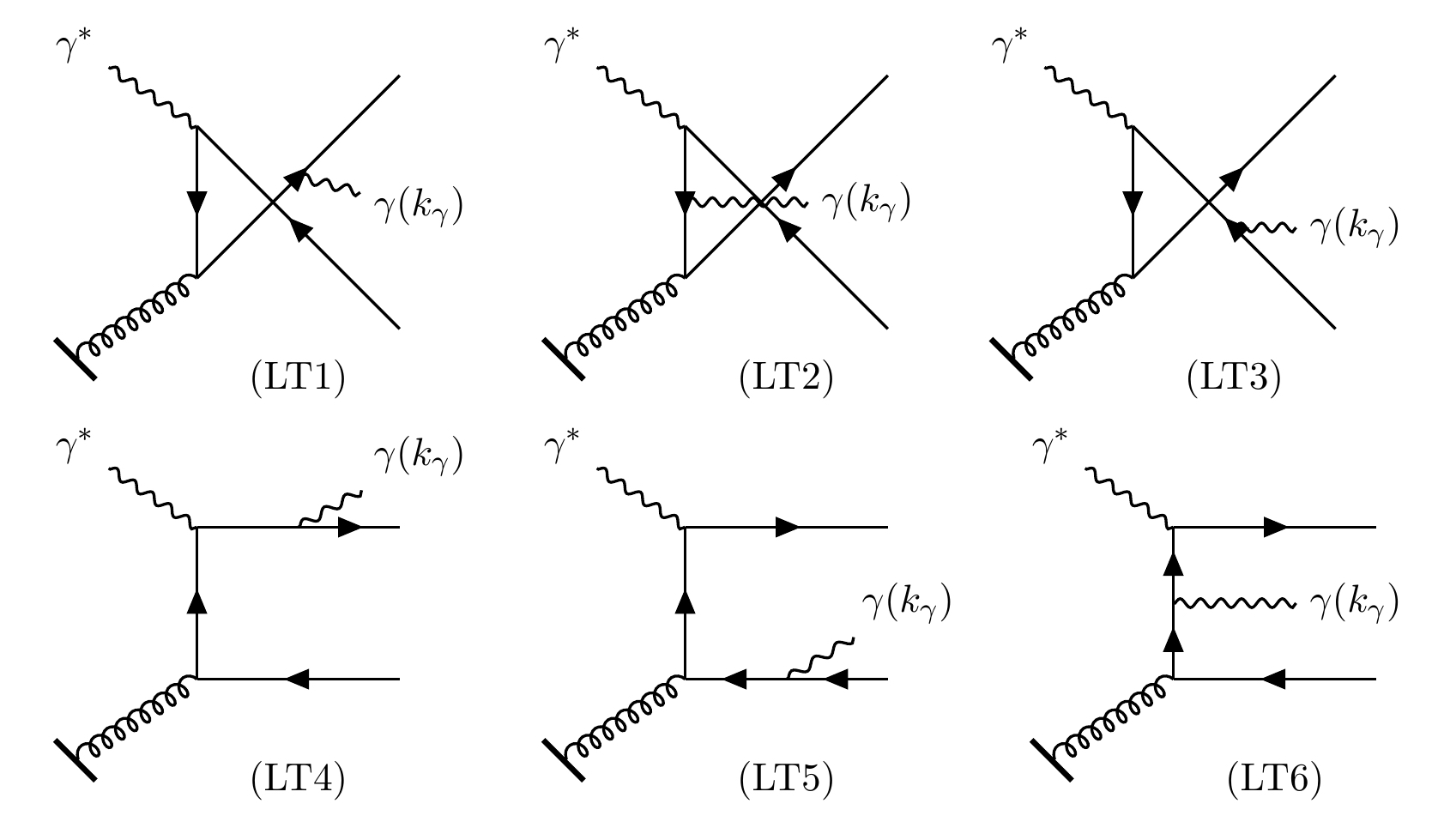
Figure 10: Photon-gluon fusion diagrams contributing to the amplitude at leading twist, $\mathcal{O}(\rho_{A})$. The nuclear source is represented by the lower bold line.

The leading twist amplitude can be written as

$$\mathcal{M}^{\text{LT}}(\mathbf{q},\mathbf{k},\mathbf{p},\mathbf{k}_{\gamma})=\epsilon^{*\alpha}(\mathbf{k}_{\gamma},\lambda)\epsilon^{\mu}(\mathbf{q},\lambda^{\prime})\mathcal{M}^{\text{LT}}_{\mu\alpha}(\mathbf{q},\mathbf{k},\mathbf{p},\mathbf{k}_{\gamma})\enskip,$$ (65)

where

$$\mathcal{M}^{\text{LT}}_{\mu\alpha}(\mathbf{q},\mathbf{k},\mathbf{p},\mathbf{k}_{\gamma})=A^{\nu}_{a,A}(P-q)m^{a}_{\alpha\mu\nu}(\mathbf{q},\mathbf{k},\mathbf{p},\mathbf{k}_{\gamma})\enskip.$$ (66)

The Fourier transform of the gluon field is given by

$$A^{\nu}_{a,A}(P-q)=2\pi g\delta^{\nu+}\delta(P^{-}-q^{-})\enskip\frac{\rho_{a,A}(\mathbf{P}_{\perp})}{\mathbf{P}_{\perp}^{2}}\enskip,$$ (67)

and

$$m^{a}_{\alpha\mu\nu}(\mathbf{q},\mathbf{k},\mathbf{p},\mathbf{k}_{\gamma})=\sum_{\beta=1}^{6}m^{\beta,a}_{\alpha\mu\nu}(\mathbf{q},\mathbf{k},\mathbf{p},\mathbf{k}_{\gamma})\enskip,$$ (68)

corresponds to the contributions from the leading twist diagrams (LT1)-(LT6), which can be individually written as

$$m^{\beta,a}_{\alpha\mu+}(\mathbf{q},\mathbf{k},\mathbf{p},\mathbf{k}_{\gamma})=\begin{cases}-ie^{2}gq^{2}_{f}\enskip\overline{u}(\mathbf{k})R^{(\beta)}_{\alpha\mu}(\mathbf{P}_{\perp})t^{a}v(\mathbf{p})\enskip,\quad\beta=1,2,3\\ +ie^{2}gq^{2}_{f}\enskip\overline{u}(\mathbf{k})R^{(\beta)}_{\alpha\mu}(\mathbf{P}_{\perp})t^{a}v(\mathbf{p})\enskip,\quad\beta=4,5,6\enskip,\end{cases}$$ (69)

where the various R-factors are given by Eqs. 21, 25 and 28 respectively. Using these relations 67 and 69 in Eq. 66, we get

$$\mathcal{M}^{\text{LT}}_{\mu\alpha}(\mathbf{q},\mathbf{k},\mathbf{p},\mathbf{k}_{\gamma})=-ie^{2}g^{2}q^{2}_{f}(2\pi)\delta(P^{-}-q^{-})\,\frac{\rho_{a,A}(\mathbf{P}_{\perp})}{\mathbf{P}_{\perp}^{2}}\,\Big{[}\overline{u}(\mathbf{k})\big{(}T^{(\bar{q})}(\mathbf{P}_{\perp})-T^{(q)}(\mathbf{P}_{\perp})\big{)}_{\mu\alpha}t^{a}v(\mathbf{p})\Big{]}\enskip.$$ (70)

Taking the modulus squared and using

$$\left\langle\rho_{A}^{a}(\mathbf{P}_{\perp})\rho_{A}^{b}(\mathbf{P}_{\perp})\right\rangle_{Y_{A}}=\frac{\delta^{ab}\mathbf{P}_{\perp}^{2}}{2\pi N_{c}C_{F}g^{2}}\enskip\phi_{Y_{A}}(\mathbf{P}_{\perp})\enskip,$$ (71)

for the correlator of color sources, we obtain

$$X^{\text{LT}}_{\mu\nu}=-\left\langle\sum_{spins}{\mathcal{M}_{\mu\alpha}^{\text{LT}}}^{*}(\mathbf{q},\mathbf{k},\mathbf{p},\mathbf{k}_{\gamma}){\mathcal{M}_{\nu}^{\text{LT}}}^{\alpha}(\mathbf{q},\mathbf{k},\mathbf{p},\mathbf{k}_{\gamma})\right\rangle=16\pi^{2}\alpha^{2}N_{c}q^{4}_{f}\enskip\overset{\sim}{X}_{\mu\nu}^{\text{LT}}\enskip,$$ (72)

where is identical to the expression in Eq. 63.

Finally, we can take the collinear limit of the leading twist expressions. In our case, this is equivalent to taking the limit $\mathbf{P}_{\perp}\rightarrow 0$ of $\Theta_{\mu\nu}(\mathbf{P}_{\perp})/\mathbf{P}^{2}_{\perp}$. In analogy to the discussion in the $p+A$ case  Gelis and Venugopalan (2004); Benic et al. (2017), we verify that the Ward identity

$$(P-q)^{\nu}m^{a}_{\alpha\mu\nu}(\mathbf{q},\mathbf{k},\mathbf{p},\mathbf{k}_{\gamma})=0\enskip,$$ (73)

is indeed satisfied. Since $P^{-}-q^{-}=0$, the Ward identity implies

$$m^{a}_{\alpha\mu+}=\frac{P_{i}m^{a}_{\alpha\mu i}}{P^{+}-q^{+}}\enskip,$$ (74)

so that $m^{a}_{\alpha\mu+}$ vanishes linearly with $\mathbf{P}_{\perp}$. Thus the limit

$$\lim_{\mathbf{P}_{\perp}\rightarrow 0}\frac{\Theta_{\mu\nu}(\mathbf{P}_{\perp})}{\mathbf{P}^{2}_{\perp}}\enskip,$$ (75)

is well-defined, leading to the collinear perturbative QCD result for the hadron tensor:

$$\overset{\sim}{X}_{\mu\nu}^{\rm{coll.}}=\frac{2\alpha_{S}\pi^{2}}{N_{c}}\enskip(2\pi)^{2}\delta^{(2)}(\mathbf{p}_{\perp}+\mathbf{k}_{\perp}+\mathbf{k}_{\gamma\perp})\enskip x_{A}f_{g,A}(x_{A},Q^{2})\lim_{\mathbf{P}_{\perp}\rightarrow 0}\frac{\Theta_{\mu\nu}(\mathbf{P}_{\perp})}{\mathbf{P}^{2}_{\perp}}\enskip.$$ (76)

Note that the l.h.s is proportional to the nuclear gluon distribution at small $x$,

$$x_{A}f_{g,A}(x_{A},Q^{2})=\frac{1}{\pi^{2}}\int_{\mathbf{l}_{1\perp}}\phi_{Y_{A}}(\mathbf{l}_{1\perp})\enskip.$$ (77)

The above result should be compared to inclusive photon production at NLO or $\mathcal{O}(\alpha_{S})$ in the power counting of pQCD, first analyzed in detail by Aurenche et. al. Aurenche et al. (1984) and later for photon plus jet cross-sections in Gehrmann-De Ridder et al. (2000); Kramer et al. (1998); Michelsen (1995). Excluding photoproduction, the NLO contributions come from two classes of inelastic diagrams; the photon-gluon fusion processes with a prompt photon in the final state and bremsstrahlung processes with a valence quark interacting directly with the virtual photon. In the power counting of CGC, the latter form a subset of the Class I processes. As clearly shown in Eq. (10) of Aurenche et al. (1984), the cross-section for photon-gluon fusion processes clearly dominate the other inelastic processes at small $x$ by virtue of being proportional to the nucleon/nuclear gluon distribution in $e+p$/$e+A$ inclusive direct photon production.

This correspondence between leading twist approximation of CGC and conventional collinearly factorized pQCD results is useful. Besides corroborating our framework in a well-defined limit, it allows one to extract subleading power corrections to the nuclear gluon distribution. Further, one recovers higher order results (in the collinear pQCD power counting) that are the dominant NLO pQCD corrections to inclusive prompt photon production in the limit when both energies and virtualities are large even though $x\ll 1$.

IV.2 Inclusive dijet cross-section in the soft photon limit

We will show here that in the infrared limit, $k_{\gamma}\rightarrow 0$, the Low-Burnett-Kroll theorem is satisfied by the inclusive photon production amplitude. Towards this end, we shall consider only the hadronic subprocesses for which the amplitude is given by Eqs. 15 and 47. In this limit, only the processes (7) and (8) (see Fig. 9) correspond to the photon being radiated after scattering from the nucleus and hence possess the desired structures

$$\frac{\not{k}+\not{k}_{\gamma}+m}{(k+k_{\gamma})^{2}-m^{2}}\quad\text{or}\quad\frac{\not{p}+\not{k}_{\gamma}-m}{(p+k_{\gamma})^{2}-m^{2}}\enskip,$$ (78)

where the denominators linearly diverge as $k_{\gamma}\rightarrow 0$

$$(p+k_{\gamma})^{2}-m^{2}\rightarrow 2p.k_{\gamma}\enskip,\qquad(k+k_{\gamma})^{2}-m^{2}\rightarrow 2k.k_{\gamma}\enskip,$$ (79)

and the numerators stay finite

$$\overline{u}(\mathbf{k})\gamma_{\alpha}(\not{k}+\not{k}_{\gamma}+m) \rightarrow 2k_{\alpha}\overline{u}(\mathbf{k})\enskip,$$

$$(\not{p}+\not{k}_{\gamma}-m)\gamma_{\alpha}v(\mathbf{p}) \rightarrow 2p_{\alpha}v(\mathbf{p})\enskip,$$ (80)

The contributions from diagrams (9) and (10) are of $\mathcal{O}(k_{\gamma}^{0})$ in the soft photon limit and are therefore subleading compared to those from diagrams (7) and (8). Combining the two leading contributions in the soft photon limit, we get

$$\mathcal{M}_{\mu}(\mathbf{q},\mathbf{k},\mathbf{p},\mathbf{k}_{\gamma})\rightarrow-(eq_{f})\epsilon^{*}_{\alpha}(\mathbf{k}_{\gamma},\lambda)\Big{(}\frac{p^{\alpha}}{p.k_{\gamma}}-\frac{k^{\alpha}}{k.k_{\gamma}}\Big{)}\mathcal{M}_{\mu}^{NR}(\mathbf{q},\mathbf{k},\mathbf{p})\enskip,$$ (81)

where $\mathcal{M}_{\mu}^{NR}(\mathbf{q},\mathbf{k},\mathbf{p})$ is the amplitude for inclusive dijet production computed in the CGC framework at small $x$ in Gelis and Jalilian-Marian (2003); Dominguez et al. (2011). The explicit expression is given by Eq. 122. It is then straightforward to calculate the differential cross-section for inclusive dijet production and express it in the familiar dipole factorized form. Details of this computation are given in Appendix B.2.

The final result can be expressed as

$$\frac{\mathrm{d}\sigma^{L,T}}{\mathrm{d}^{3}k\mathrm{d}^{3}p} =\alpha\,q_{f}^{2}N_{c}\delta(q^{-}-p^{-}-k^{-})\int\frac{\mathrm{d}^{2}\mathbf{x}_{\perp}}{(2\pi)^{2}}\frac{\mathrm{d}^{2}\mathbf{x^{\prime}}_{\perp}}{(2\pi)^{2}}\frac{\mathrm{d}^{2}\mathbf{y}_{\perp}}{(2\pi)^{2}}\frac{\mathrm{d}^{2}\mathbf{y^{\prime}}_{\perp}}{(2\pi)^{2}}\enskip e^{-i\mathbf{k}_{\perp}.(\mathbf{x}_{\perp}-\mathbf{x^{\prime}}_{\perp})}e^{-i\mathbf{p}_{\perp}.(\mathbf{y}_{\perp}-\mathbf{y^{\prime}}_{\perp})}$$

$$\times\sum_{\alpha,\beta}\psi^{L,T}_{\alpha\beta}(q^{-},z,|\mathbf{x}_{\perp}-\mathbf{y}_{\perp}|)\enskip\psi^{L,T*}_{\alpha\beta}(q^{-},z,|\mathbf{x^{\prime}}_{\perp}-\mathbf{y^{\prime}}_{\perp}|)\times\Xi(\mathbf{x}_{\perp},\mathbf{y}_{\perp};\mathbf{x^{\prime}}_{\perp},\mathbf{y^{\prime}}_{\perp})\enskip,$$ (82)

where $\Xi$ is given by Eq. 52. Our result exactly matches that obtained previously in Dominguez et al. (2011) (see Eq. (22) of the same) for inclusive dijet production at small $x$. This is a versatile result, because as argued in Dominguez et al. (2011, 2012), measurements of this cross-section in $e+A$ collisions provides a direct channel to extract the nuclear Weizsäcker-Williams distribution McLerran and Venugopalan (1999); Kovchegov and Mueller (1998).

IV.3 The dressed fermion propagator

In this subsection, we will outline a convenient modification of the momentum space Feynman rules for the fermion propagator in the background classical color field which enables one to efficiently recover our results thus far. As we shall also shortly discuss, this modification is valid for the dressed gluon propagator as well.

We begin by observing that the factor of unity subtracted from the Wilson line in the effective vertex for the dressed fermion propagator (given in Eq. 11) imposes the requirement that the quark (antiquark) has to necessarily scatter off the nucleus. If we now redefine the effective vertex as

$$\overset{\sim}{\mathcal{T}}_{ji}(q,p)=\pm(2\pi)\delta(p^{-}-q^{-})\gamma^{-}\int\mathrm{d}^{2}\mathbf{x}_{\perp}e^{i(\mathbf{q}_{\perp}-\mathbf{p}_{\perp}).\mathbf{x}_{\perp}}\tilde{U}^{(\pm)}(\mathbf{x}_{\perp})_{ji}\enskip,$$ (83)

where the plus (minus) signs again correspond respectively to insertions on quark (antiquark) line, this includes the possibility of “no scattering” off the quark or antiquark line. The LO amplitude expression in Eq. 47 then has a simple physical interpretation. The first part proportional to $\tilde{U}(\mathbf{x}_{\perp})\tilde{U}^{\dagger}(\mathbf{y}_{\perp})$ represents all possible scatterings of the quark and antiquark off the nucleus, including the case in which they do not scatter at all. We can represent this diagrammatically as the sum of contributions from processes labeled (7)-(10) in Fig. 9 but with the blobs replaced by crossed dots as shown in Fig. 11.

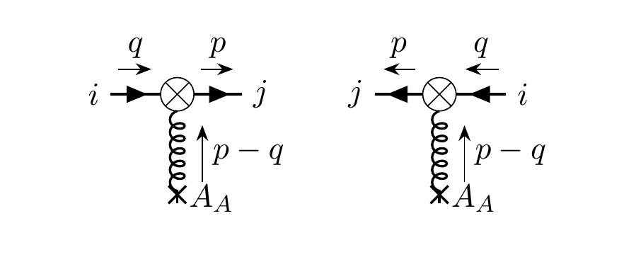
Figure 11: Diagrammatic representation of the modified effective vertices for the quark and antiquark respectively. The crossed dots represent all possible scatterings off the classical color field of the nucleus including the case of no scattering. The vertex factors are given by Eq. 83.

The second part which is proportional to unity gives the “no scattering” contribution and must be subtracted to get the physical result. As we will demonstrate in further detail in Appendix C, this seemingly simple modification offers a significant advantage because it is sufficient to compute fewer diagrams in the LO computation than previously. An identical argument holds for the effective vertex for the dressed gluon propagator. These modified quark and gluon vertices will prove very valuable in computations at NLO and higher orders.

V Components of the NLO computation

V.1 Advantages of the “wrong” light cone gauge

Albeit computations of physical observables are gauge independent, an appropriate gauge choice can result in a significant simplification of our path to the final result. In DIS, an attractive gauge choice, in the infinite momentum frame (IMF) where $P^{+}_{N}\rightarrow\infty$, is the light cone gauge $A^{+}=0$ . This follows from the operator definition of parton distribution functions (PDFs), which are defined respectively for quark and gluon fields as Diehl (2003)

$$F^{q} =\frac{1}{2}\int\frac{\mathrm{d}z^{-}}{2\pi}\enskip e^{ixP^{+}_{N}z^{-}}\langle P_{N}|\enskip\bar{q}\Big{(}-\frac{z}{2}\Big{)}\gamma^{+}W\Big{(}-\frac{z^{-}}{2},\frac{z^{-}}{2}\Big{)}q\Big{(}\frac{z}{2}\Big{)}\enskip|P_{N}\rangle{\Bigg{|}}_{z^{+}=0,\mathbf{z}_{\perp}=0}\enskip,$$

$$F^{g} =\frac{1}{P^{+}_{N}}\int\frac{\mathrm{d}z^{-}}{2\pi}\enskip e^{ixP^{+}_{N}z^{-}}\langle P_{N}|\enskip G^{+\mu}\Big{(}-\frac{z}{2}\Big{)}W\Big{(}-\frac{z^{-}}{2},\frac{z^{-}}{2}\Big{)}{G_{\mu}}^{+}\Big{(}\frac{z}{2}\Big{)}\enskip|P_{N}\rangle{\Bigg{|}}_{z^{+}=0,\mathbf{z}_{\perp}=0}\enskip.$$ (84)

In the IMF, the $W$’s are lightlike gauge links which are defined to be

$$W(a,b)=\mathcal{P}_{-}\text{exp}\Big{(}ig\int_{b}^{a}\mathrm{d}x^{-}A^{+}\Big{)}\enskip.$$ (85)

These are of course unity in in $A^{+}=0$ gauge. In a covariant representation, with off-shell partons and on-shell hadrons, a simple interpretation of the PDFs in terms of Green functions is possible in this gauge Diehl (2003) . Similarly, in a noncovariant representation with on-shell partons, or in other words, light cone quantization Kogut and Soper (1970); Bjorken et al. (1971); Brodsky and Robertson (1995); Brodsky et al. (1998); Venugopalan (1998), a number density interpretation of the quark and gluon PDFs is manifest in $A^{+}=0$ gauge.

Though $A^{+}=0$ is the right gauge choice for the reasons outlined, it turns out that the “wrong” gauge choice of $A^{-}=0$ is the right one for computations in shock wave background fields. Firstly, we note that in the IMF $P^{+}_{N}\rightarrow\infty$, the only large component of the current density is $J^{+}$ with other components suppressed by $1/P^{+}_{N}$. The current conservation equation is therefore equivalent to

$$D_{+}J^{+}=0\enskip.$$ (86)

It ensures that $J^{+}$ is independent of the light cone time $x^{+}$, or equivalently, is a static charge on the light cone. This is implicitly assumed in Eq. 8 and in the subsequent analysis. The solution of the classical Yang-Mills equations in $A^{-}=0$ gauge gives McLerran and Venugopalan (1994a, b)

$$A^{+}=0,\enskip F^{ij}=0\qquad\text{with}\enskip A^{+},A^{i}\,\,x^{+}\,\,\text{independent}\enskip,$$ (87)

a solution that is also of course valid in the right light cone gauge $A^{+}=0$.

However unlike $A^{+}=0$ gauge, $A^{-}=0$ gauge is related to the Lorenz gauge $\partial_{\mu}A^{\mu}=0$ by a simple gauge transformation. Note that our LO computations thus far were in the latter gauge, where the fermion propagator had a particularly simple structure McLerran and Venugopalan (1999); Venugopalan (1999). Most importantly, as noted previously Ayala et al. (1995, 1996), the structure of the small fluctuation propagator in $A^{-}=0$ gauge is far simpler than that in $A^{+}=0$ gauge. Further, this dressed gluon propagator, when transformed to Lorenz gauge, has a structure that is identical to that of the fermion propagator.

Leading order computations in shock wave backgrounds, comparing and contrasting results in the Lorenz and $A^{-}=0$ light cone gauge have been performed previously in the context of $p+A$ collisions. While it was noted that results for gluon production in $A^{-}=0$ gauge Gelis and Mehtar-Tani (2006) are less cumbersome relative to those in Lorenz gauge Blaizot et al. (2004a), there is no particular virtue of one or the other gauge for quark pair production Blaizot et al. (2004b) or inclusive photon production Benic et al. (2017). Because the shock wave background fields in the two gauges are simply related, intermediate steps may be performed more efficiently in Lorenz gauge before transforming the final result to $A^{-}=0$ gauge.

V.2 Gluon “shock wave” propagator in $A^{-}=0$ gauge

We will begin by rederiving Ayala et al. (1995) the shock wave gluon propagator in $A^{-}=0$ gauge. We can split the gauge field into a classical background field piece (parametrically of order $1/g$) and a small fluctuation piece (of order unity) as

$$A^{\mu}(x)=B^{\mu}(x)+b^{\mu}(x)\enskip.$$ (88)

Here $B^{\mu}(x)$ is the classical background field with the components

$$B^{+}(x)=0,\enskip B^{-}(x)=0,\enskip B^{i} =\theta(x^{-})\kappa^{i}(\mathbf{x}_{\perp})\enskip,\qquad i=1,2\enskip,$$

$$\text{where}\quad\kappa^{i}(\mathbf{x}_{\perp}) =\frac{i}{g}\enskip U(\mathbf{x}_{\perp})\partial^{i}U^{\dagger}(\mathbf{x}_{\perp})\enskip,$$ (89)

and $U$ is the Wilson line in the adjoint representation of $SU(N_{c})$,

$$U(\mathbf{x_{\perp}})=\mathcal{P}_{-}\text{exp}\left[-ig^{2}\int_{-\infty}^{+\infty}\mathrm{d}z^{-}\frac{1}{\nabla^{2}_{\perp}}\rho_{A}^{a}(z^{-},\mathbf{x_{\perp}})T^{a}\right]\enskip.$$ (90)

The equations of motion for the small fluctuation field $b(x)$ are

$$\Big{(}D(B)^{2}g^{\mu\nu}-D^{\mu}(B)D^{\nu}(B)\Big{)}b_{\nu}-2F^{\mu\nu}b_{\nu}=0\enskip.$$ (91)

Specifically, for the transverse fields, we have a sourceless Klein-Gordon equation

$$[2\partial^{+}\partial^{-}-\mathbf{D}_{\perp}^{2}(B)]\enskip b^{i}(x)=0\enskip,$$ (92)

after fixing the residual gauge freedom with the Gauss’ law constraint $D^{\mu}(B)b_{\mu}=0$ . Taking $\mu=-$ in Eq. 91, we get another sourceless equation

$$\partial^{-}\Big{(}\partial^{-}b^{+}-\mathbf{D}_{\perp}.\mathbf{b}_{\perp}\Big{)}=0\enskip,$$ (93)

which is the Gauss’ law constraint imposed on initial field configurations Gelis et al. (2007, 2008a, 2008b).

Finally, using the above constraint to write

$$b^{+}=\frac{1}{\partial^{-}}\enskip\mathbf{D}_{\perp}.\mathbf{b}_{\perp}\enskip,$$ (94)

and keeping in mind the discontinuity of the spatial covariant derivative operator at $x^{-}=0$, we can verify that Eqs. 92 and 94 are consistent with the final small fluctuation equation

$$[2\partial^{+}\partial^{-}-\mathbf{D}_{\perp}^{2}(B)]\enskip b^{+}=-2\delta(x^{-})\enskip\kappa^{i}(\mathbf{x}_{\perp})b_{i}\enskip.$$ (95)

The transverse field is then assumed to be a simple plane wave for $x^{-}<0$ and a linear superposition of plane waves for $x^{-}>0$. This is done in a manner to ensure continuity of the fields across $x^{-}=0$, which again is possible because of the absence of delta function singularities in the above equations at $x^{-}=0$. The expressions for the Green’s functions for the small fluctuations thus obtained are given in the next subsection.

In contrast, in the right light cone gauge $A^{+}=0$, the discontinuity of the fields at the origin and the corresponding singular structure of the electric fields do not allow one to simply integrate the equations of motion. Hence it is convenient to first obtain the small fluctuation Green functions in $A^{-}=0$ gauge and then, if required, gauge transform the results to $A^{+}=0$. The expressions for the propagator in $A^{+}=0$ gauge are complicated and not of relevance in our NLO computation.

Following the procedure outlined above and using the identity

$$\tilde{U}(\mathbf{x}_{\perp})t^{a}\tilde{U}^{\dagger}(\mathbf{x}_{\perp})=t^{b}U^{ba}(\mathbf{x}_{\perp})\enskip,$$ (96)

we can express the transverse components of the fluctuation field as McLerran and Venugopalan (1994c); Ayala et al. (1995),

$$b^{i}(x)=e^{ip.x}\eta^{i}\Big{[}\theta(-x^{-})t^{a}+\theta(x^{-})\int\frac{\mathrm{d}^{2}\mathbf{q}_{\perp}}{(2\pi)^{2}}\int\mathrm{d}^{2}\mathbf{z}_{\perp}\enskip e^{-i(\mathbf{q}_{\perp}-\mathbf{p}_{\perp}).(\mathbf{x}_{\perp}-\mathbf{z}_{\perp})}e^{i(\mathbf{q}_{\perp}^{2}-\mathbf{p}_{\perp}^{2})\frac{x^{-}}{2p^{-}}}\enskip t^{c}\Big{(}U(\mathbf{x}_{\perp})U^{\dagger}(\mathbf{z}_{\perp})\Big{)}^{ca}\Big{]}\enskip,$$ (97)

where $\eta^{i}$ is a unit vector. Using the above expression for $b^{i}$, we get

$$b^{+}(x)=\frac{1}{\partial_{y^{+}}}\enskip[\mathbf{D}_{\perp},\mathbf{b}_{\perp}]=\frac{1}{\partial_{y^{+}}}\enskip\Big{[}e^{ip.x}\eta^{j}\Bigl{\{}\theta(-x^{-})ip^{j}t^{a}+ \theta(x^{-})\int\frac{\mathrm{d}^{2}\mathbf{q}_{\perp}}{(2\pi)^{2}}\int\mathrm{d}^{2}\mathbf{z}_{\perp}\enskip e^{-i(\mathbf{q}_{\perp}-\mathbf{p}_{\perp}).(\mathbf{x}_{\perp}-\mathbf{z}_{\perp})}e^{i(\mathbf{q}_{\perp}^{2}-\mathbf{p}_{\perp}^{2})\frac{x^{-}}{2p^{-}}}$$

$$\times i(p^{j}+q^{j})t^{c}\Big{(}U(\mathbf{x}_{\perp})U^{\dagger}(\mathbf{z}_{\perp})\Big{)}^{ca}\Bigr{\}}\Big{]}\enskip.$$ (98)

The small fluctuation gluon propagator in coordinate space is defined as

$$G^{\mu\nu;ab}(x,y)=\left\langle b^{\mu,a}(x)b^{\nu,b}(y)\right\rangle\enskip.$$ (99)

The nonzero components of the propagator in this gauge are $G^{++}$, $G^{+i}$, $G^{i+}$ and $G^{ij}$. Using the expression for $G^{ij}$ in McLerran and Venugopalan (1994c); Ayala et al. (1995) and Eq. 96, it is straightforward to derive the following alternate expressions useful for momentum space calculations:

$$G^{ij;ab}(x,y) =g(x^{-},\mathbf{x}_{\perp})\enskip G^{ij;ab}_{0}(x,y)\enskip g^{\dagger}(y^{-},\mathbf{y}_{\perp})-\int\mathrm{d}^{4}z\enskip\delta(z^{-})g(x^{-},\mathbf{x}_{\perp})\Bigl{\{}\theta(x^{-})\theta(-y^{-})[U^{\dagger}(\mathbf{z}_{\perp})-1]$$

$$-\theta(-x^{-})\theta(y^{-})[U(\mathbf{z}_{\perp})-1]\Bigr{\}}_{cd}g^{\dagger}(y^{-},\mathbf{y}_{\perp})\enskip G^{ik;ac}_{0}(x,z)(-i2\partial_{z^{+}})G^{lj;db}_{0}(z,y)\delta_{kl}\enskip,$$ (100)

where

$$G_{0}^{\mu\nu;ab}(x,y)=\int\frac{\mathrm{d}^{4}p}{(2\pi)^{4}}\enskip e^{ip.(x-y)}\frac{i}{p^{2}+i\varepsilon}\Big{(}-g^{\mu\nu}+\frac{p^{\mu}n^{\nu}+p^{\nu}n^{\mu}}{n.p}\Big{)}\delta^{ab},\qquad n^{\mu}=\delta^{\mu+}\enskip,$$ (101)

is the free gluon propagator in $A^{-}=0$ gauge. Further,

$$g(x^{-},\mathbf{x}_{\perp})=\theta(-x^{-})+\theta(x^{-})U(\mathbf{x}_{\perp})\enskip,$$ (102)

is a gauge transformation matrix that transforms the background field $B^{\mu}(x)$ to Lorenz gauge in which it is a singular field having only a ‘plus’ component. The same matrix, albeit in the fundamental representation, appears while calculating the fermion propagator McLerran and Venugopalan (1999) in the background classical field.

The momentum space expression for the gluon propagator in $A^{-}=0$ gauge with the background field $B(x)$ in Lorenz gauge can be expressed as

$$G^{ij;ab}(p,p^{\prime})=(2\pi)^{4}\delta^{(4)}(p-p^{\prime})\enskip G^{ij;ab}_{0}(p)+G^{ik;ac}_{0}(p)\enskip{\mathcal{T}}_{kl;cd}(p,p^{\prime})\enskip G^{lj;db}_{0}(p^{\prime})\enskip,$$ (103)

where

$${\mathcal{T}}_{ij;ab}(p,p^{\prime})=2\pi\delta(p^{-}-p^{\prime-})\,(2p^{-})\text{sign}(p^{-})\int\mathrm{d}^{2}\mathbf{z}_{\perp}\enskip e^{i(\mathbf{p}_{\perp}-\mathbf{p^{\prime}}_{\perp}).\mathbf{z}_{\perp}}[U^{\text{sign}(p^{-})}(\mathbf{z}_{\perp})-1]_{ab}\delta_{ij}\enskip.$$ (104)

One can similarly derive the following momentum space relations for the other nonzero components of $G^{\mu\nu}$:

$$G^{++;ab}(p,p^{\prime}) =(2\pi)^{4}\delta^{(4)}(p-p^{\prime})\enskip G^{++;ab}_{0}(p)+G^{+i;ac}_{0}(p)\enskip{\mathcal{T}}_{ij;cd}(p,p^{\prime})\enskip G^{j+;db}_{0}(p^{\prime})\enskip,$$

$$G^{i+;ab}(p,p^{\prime}) =(2\pi)^{4}\delta^{(4)}(p-p^{\prime})\enskip G^{i+;ab}_{0}(p)+G^{ij;ac}_{0}(p)\enskip{\mathcal{T}}_{jk;cd}(p,p^{\prime})\enskip G^{k+;db}_{0}(p^{\prime})\enskip.$$ (105)

The general form for the small fluctuation propagator in momentum space and in $A^{-}=0$ gauge can be compactly expressed as

$$G^{\mu\nu;ab}(p,p^{\prime})=(2\pi)^{4}\delta^{(4)}(p-p^{\prime})\enskip G^{\mu\nu;ab}_{0}(p)+G^{\mu\rho;ac}_{0}(p)\enskip{\mathcal{T}}_{\rho\sigma;cd}(p,p^{\prime})\enskip G^{\sigma\nu;db}_{0}(p^{\prime})\enskip,$$ (106)

where the effective vertex of the dressed gluon shock wave is given by

$${\mathcal{T}}_{\mu\nu;ab}(p,p^{\prime})=-2\pi\delta(p^{-}-p^{\prime-})\,(2p^{-})g_{\mu\nu}\enskip\text{sign}(p^{-})\int\mathrm{d}^{2}\mathbf{z}_{\perp}\enskip e^{i(\mathbf{p}_{\perp}-\mathbf{p^{\prime}}_{\perp}).\mathbf{z}_{\perp}}[U^{\text{sign}(p^{-})}(\mathbf{z}_{\perp})-1]_{ab}\enskip,$$ (107)

a form identical to (with the subsitution of the fundamental Wilson line with its adjoint counterpart) the dressed fermion effective vertex. While the gluon shock wave propagator in $A^{-}=0$ gauge was first derived in McLerran and Venugopalan (1994c); Ayala et al. (1995), this form for the propagator in momentum space is given in a later paper by Balitsky and Belitsky Balitsky and Belitsky (2002) albeit it is also implicit in Hebecker and Weigert (1998); McLerran and Venugopalan (1999).

The discussion in Sec. IV.3 however suggests that we should modify the effective gluon vertex to include the “no scattering” contribution by omitting the unit matrix in Eq. 107 above; the modified vertex we will use henceforth in computations is

$$\overset{\sim}{\mathcal{T}}_{\mu\nu;ab}(p,p^{\prime})=-2\pi\delta(p^{-}-p^{\prime-})\,(2p^{-})g_{\mu\nu}\enskip\text{sign}(p^{-})\int\mathrm{d}^{2}\mathbf{z}_{\perp}\enskip e^{i(\mathbf{p}_{\perp}-\mathbf{p^{\prime}}_{\perp}).\mathbf{z}_{\perp}}U^{\text{sign}(p^{-})}_{ab}(\mathbf{z}_{\perp})\enskip.$$ (108)

To summarize, higher order all-twist computations at small $x$ can be performed with the conventional Feynman rules of covariant perturbation theory albeit with the dressed quark and gluon effective vertices shown in Fig. 12.

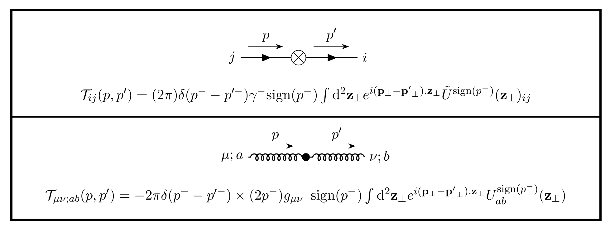
Figure 12: Diagrammatic representation of the fermion (top) and gluon (bottom) effective vertices. Here, and henceforth, the ‘tilde’ factors in Eqs. 83 and 108 are dropped.

V.3 Processes contributing to the NLO amplitude

Having outlined the necessary components for the computation of the inclusive photon amplitude to NLO, we will discuss here the relevant NLO processes. The general ideas were already presented in the introduction of this paper and we will elaborate further on that discussion. To begin with, the perturbative expansion in Eq. 3 of the expectation value of a general operator $\mathcal{O}$ calculated for a particular source charge density configuration $\rho_{A}$ can be expanded out to next-to-next-to-leading order (NNLO) as

$$\mathcal{O}[\rho_{A}] =\underbrace{f^{0}_{0j}(g\rho_{A})^{j}}_{\textrm{LO}}+\underbrace{f^{0}_{1j}(g\rho_{A})^{j}\alpha_{S}+f^{1}_{1j}(g\rho_{A})^{j}\alpha_{S}\enskip\text{ln}(1/x)}_{\textrm{NLO}}$$

$$+\underbrace{f^{0}_{2j}(g\rho_{A})^{j}\alpha_{S}^{2}+f^{1}_{2j}(g\rho_{A})^{j}\alpha_{S}^{2}\enskip\text{ln}(1/x)+f^{2}_{2j}(g\rho_{A})^{j}\alpha^{2}_{S}\enskip\text{ln}^{2}(1/x)}_{\textrm{NNLO}}+\ldots\enskip,$$ (109)

where the repeated indices are assumed to be summed over. For the differential cross-section for inclusive photon production, at each order in perturbation theory, there are contributions to the small $x$ evolution of the random color sources (encoded in the dipole and quadrupole Wilson line correlators given by Eq. 52). These are enhanced by logarithms in $x$ and when $\alpha_{S}\ln(1/x)\sim 1$, they complicate the naive power counting. In addition, we will have non-log enhanced perturbative corrections to the light cone wavefunction for the virtual photon that fluctuates into a quark-antiquark dipole (as well as ancillary complications due to the photon in the final state) that should be combined with the $\ln(1/x)$ contributions systematically. It is therefore efficient to reexpress the generic expansion in Eq. 109 by factorizing the cross-section into a coefficient term and a matrix element of Wilson line correlators between nuclear wavefunctions, at each order in $\alpha_{S}$, as

$$\mathrm{d}\sigma[\rho_{A}] =\underbrace{\mathcal{C}_{\text{LO}}\otimes\mathrm{d}\hat{\sigma}_{\text{LO}}}_{\alpha_{S}^{0}.\alpha_{S}^{0}}+\underbrace{\mathcal{C}_{\text{LO}}\otimes\mathrm{d}\hat{\sigma}_{\text{LLx}}}_{\alpha_{S}^{0}.\alpha_{S}\text{ln}(1/x)}+\underbrace{\mathcal{C}_{\text{NLO}}\otimes\mathrm{d}\hat{\sigma}_{\text{NLO}}}_{\alpha_{S}.\alpha_{S}^{0}}$$

$$+\underbrace{\mathcal{C}_{\text{NLO}}\otimes\mathrm{d}\hat{\sigma}_{\text{LLx}}}_{\alpha_{S}.\alpha_{S}\text{ln}(1/x)}+\underbrace{\mathcal{C}_{\text{LO}}\otimes\mathrm{d}\hat{\sigma}_{\text{NNLx}}}_{\alpha^{0}_{S}.\alpha^{2}_{S}\text{ln}(1/x)}+\ldots\enskip.$$ (110)

We computed the first term in the r.h.s of the above equation in the previous sections. The second term is given by contributions from the diagrams of the type depicted in Fig. 4. For $\alpha_{S}\,\text{ln}(1/x)\sim 1$, these contributions are as large as the LO contribution and can be absorbed in the LO result by a redefinition of the weight functional $W$. The resulting LLx RG equation (the JIMWLK equation) efficiently sums such leading contributions to all orders of perturbation theory while preserving the structure of the LO result.

The third term appearing in Eq. 110 represents genuine $\alpha_{S}$ suppressed contributions that do not take into account the small $x$ evolution of the sources. In addition to the real emission diagrams shown in Figs. 5 and 18, there are contributions from loop graphs depicted by the second and third representative diagrams in Fig. 5. Since the cross-section for inclusive gluon production in DIS was computed previously Kovchegov and Tuchin (2002) at small $x$, taking the soft-photon limit to the real emission contributions will provide in principle a check of our results. The complete calculation of this term will give the next order correction $\mathcal{C}_{\text{NLO}}$ to the LO coefficient function or “impact factor” $\mathcal{C}_{\text{LO}}$. It is worth mentioning here that the $\hat{\sigma}_{\text{NLO}}$ has a different correlator structure than $\hat{\sigma}_{\text{LO}}$ due to the additional adjoint Wilson lines and hence the distinct nomenclature. The overall contribution of the third term in Eq. 110 is strongly subleading at small $x$.

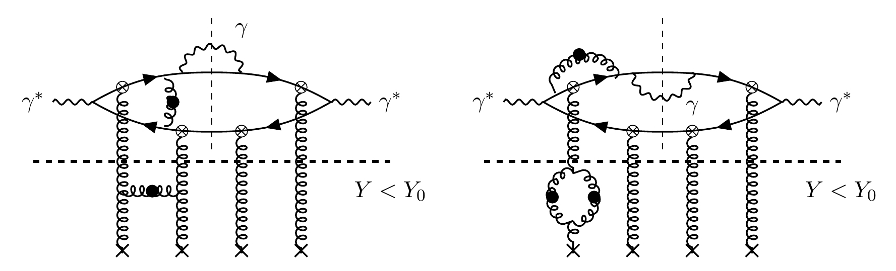
Figure 13: NNLO diagrams that are effectively $\alpha_{S}$ in “size” for $\alpha_{S}\text{ln}(1/x)\sim 1$ at small $x$. The rapidity separation between fast sources and slow fields is shown clearly. Integration over modes with $Y>Y_{0}$ is represented by the loops in the upper part of the figure. The contributions below the rapidity cut are part of the LLx evolution of the color sources. See text for more details.

The two terms in the second line of Eq. 110 are part of the NNLO contributions to inclusive photon production but are potentially quantitatively important because they are effectively of order $\alpha_{S}$ when $\alpha_{S}\ln(1/x)\sim 1$; these form the next-to-leading-log (NLLx) contribution to the cross-section. Under our RG ideology, the two terms can be considered separately. The first term in the second line of Eq. 110 is represented by the diagrams in Fig. 13. The dashed horizontal line represents the rapidity scale $Y_{0}$ separating the classical fields that interact with the $q\bar{q}\gamma$ system from the static color sources RG evolved by the LLx JIMWLK equation from the target. The two diagrams shown are respectively the real and virtual contributions that are characteristic of the terms that generate the JIMWLK kernel. The computation of the NLO impact factor (above the $Y_{0}$ cut) using the techniques developed here is in progress and will be reported in a follow-up paper Roy and Venugopalan . A highly nontrivial check will be to reproduce the NLO impact factor for fully inclusive DIS Bartels et al. (2001, 2002a, 2002b); Balitsky and Chirilli (2011); Beuf (2012, 2016, 2017); Hanninen et al. (2017) that should be recovered in the soft photon limit. It will also be important for the consistency of the framework to demonstrate JIMWLK factorization by explicit computation.

The final term in Eq. 110 is represented by the diagrams in Fig. 14. In this case, there are no radiative corrections above the rapidity cut and the dynamics is described by the LO impact factor. The contributions shown below the cut correspond to NLO contributions to the JIMWLK kernel. These have been computed previously Balitsky and Chirilli (2008, 2013) (see also Grabovsky (2013); Kovner et al. (2014)) and can therefore be used to construct the NLLx result for inclusive photon production in $e+A$ collisions. We note that NLLx corrections have recently been implemented for numerical computations in fully inclusive DIS Ducloue et al. (2017a).

An advantage of our approach is that it is fully implemented in momentum space; many shock wave computations use a mixture of momentum and coordinate space variables that is cumbersome. This is especially so in computing running coupling contributions Balitsky and Chirilli (2008); Kovchegov and Weigert (2007, 2008) where coordinate space prescriptions can be problematic as noted in Ducloue et al. (2017b). In our framework, there is no need to switch back and forth; all computations can be realized fully in momentum space with our modified Feynman rules. These issues will be be addressed in future work.

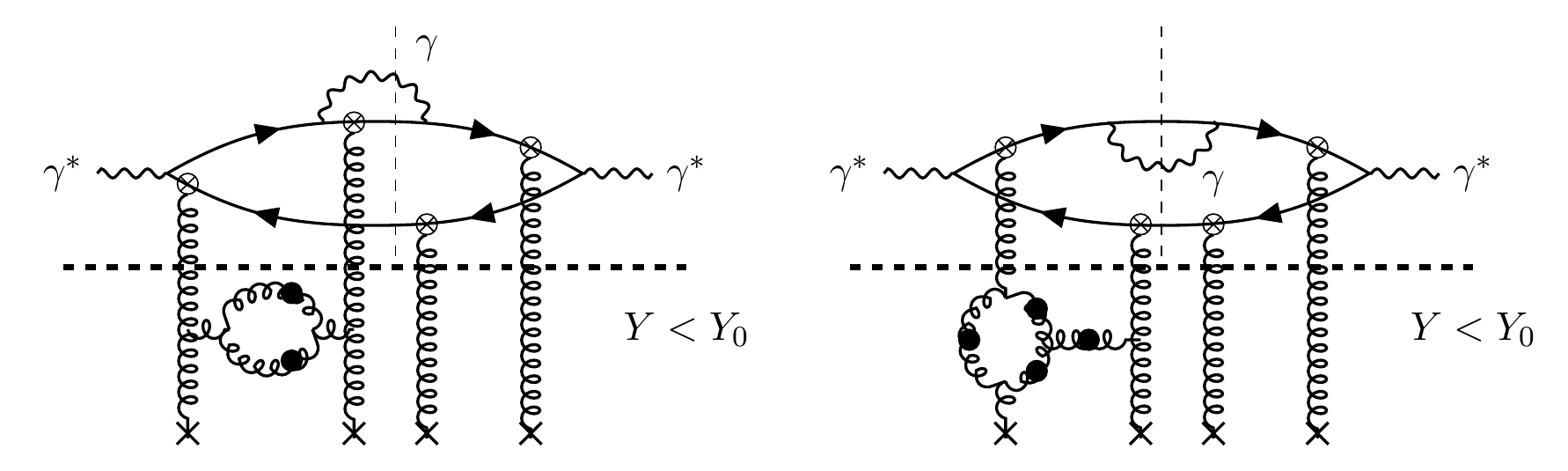
Figure 14: NNLO diagrams that are effectively $\alpha_{S}$ in “size” for $\alpha_{S}\text{ln}(1/x)\sim 1$ at small $x$. These diagrams contribute to the NLO JIMWLK kernel.

VI Summary and outlook

We presented in this paper a first computation of inclusive photon production in $e+A$ DIS at small $x$ within the CGC EFT. At LO, the cross-section is directly proportional to universal gauge invariant dipole and quadrupole Wilson line correlators which are ubiquitous in final states that are measured in high energy $p+A$ collisions and potentially in $e+A$ collisions at a future Electron-Ion Collider (EIC). Indeed, since inclusive photon production in DIS has photons in both the initial and final states, it holds promise of being a clean golden channel for unambiguous discovery of gluon saturation, complementary to other $e+A$ DIS measurements Accardi et al. (2016); Aschenauer et al. (2017). In the soft photon limit, we recover the inclusive DIS dijet cross-section derived previously in Dominguez et al. (2011). As argued there, this dijet $e+A$ channel may provide direct access to the nuclear Weizsäcker-Williams gluon distribution.

We next discussed the structure of dominant small $x$ contributions to the inclusive photon cross-section at next-to-leading order and next-to-next-to-leading order. The essential ingredients here are the dressed quark and gluon propagators and the corresponding effective vertices in the shock wave classical background field of a nucleus at high energies. These effective vertices are proportional to the respective fundamental and adjoint Wilson lines that carry information about all-twist gluon correlations in the nucleus. The structure of the quark and gluon dressed propagators is remarkably simple in the “wrong” light cone gauge $A^{-}=0$ and therefore permits efficient higher order computations. The computations are further simplified by exploiting the natural separation between static sources and dynamical gauge fields in the MV model and the JIMWLK RG treatment thereof. In particular, the cross-section can be factorized into impact factor contributions that are convoluted with the RG evolution of products of lightlike Wilson lines. The nontrivial ingredients that need to be computed are the NLO impact factor for inclusive photon production and the NLLx RG evolution of the Balitsky-JIMWLK hierarchy of Wilson line correlators. While the latter is known, the former needs to be determined; these computations are in progress and will be reported on separately Roy and Venugopalan .

We note that, motivated by collider experiments, small $x$ computations in the gluon saturation regime are increasingly to next-to-leading order accuracy. Some examples of the studies being performed include, besides inclusive DIS Ducloue et al. (2017a), DIS diffractive dijet production Boussarie et al. (2014, 2016) and exclusive light vector meson production Boussarie et al. (2017), single inclusive forward hadron production in $p+p$ and $p+A$ collisions Chirilli et al. (2012a, b); Altinoluk et al. (2016); Iancu et al. (2016) and more recently inclusive photon production in $p+A$ collisions Benic and Fukushima (2017); Benic et al. (2017). Looking further ahead, we believe that the momentum space methods discussed here can exploited to make progress in these and related computations.

The forms of the shock wave propagators first derived in McLerran and Venugopalan (1994c); Ayala et al. (1995), and their expressions in terms of effective vertices McLerran and Venugopalan (1999); Balitsky and Belitsky (2002), are identical to the quark-quark-reggeon and gluon-gluon-reggeon propagators Caron-Huot (2015); Bondarenko et al. (2017); Hentschinski (2018) in Lipatov’s reggeon field theory Lipatov (1997). We have shown here that the slightly modified quark and gluon effective vertices in Eqs. 83 and 108 significantly simplify the computation of DIS inclusive photon production. Because of the form of the shock wave propagators, our results are equally valid for leading twist or all-twist computations. It would therefore be interesting to see if our modified Feynman rules are useful in simplifying multiloop leading twist computations in the Regge limit Caron-Huot et al. (2017); Del Duca et al. (2018) or perhaps, conversely and more interestingly, results derived in those cases applied to advance computations in the saturation regime of high parton densities.

VII Appendix

Appendix A Notations and conventions

The metric used is the $-2$ metric, $\hat{g}=diag(+1,-1,-1,-1)$, where the ‘carat’ denotes quantities in usual spacetime coordinates. The light cone coordinates are defined as

$$x^{+}=\frac{\hat{x}^{0}+\hat{x}^{3}}{\sqrt{2}},\quad x^{-}=\frac{\hat{x}^{0}-\hat{x}^{3}}{\sqrt{2}}\enskip,$$

with the transverse coordinates remaining the same and transforming as in Minkowski space. The same definition holds for the gamma matrices $\gamma^{+}$ and $\gamma^{-}$ with the Dirac algebra given by

$$\{\gamma^{\mu},\gamma^{\nu}\}=2g^{\mu\nu}\enskip,$$ (111)

where $g^{+-}=g^{-+}=1$ and $g^{ij}=-\delta^{ij}$ ($i,j=1,2$) are the nonzero entries of the metric tensor. In this convention, $a.b=a^{+}b^{-}+a^{-}b^{+}-\mathbf{a}_{\perp}.\mathbf{b}_{\perp}$ and $a_{+}=a^{-}$, $a_{i}=-a^{i}$.

Appendix B Gauge invariance and soft-photon factorization at LO

The first part of this appendix provides a proof of the Ward identity for the final state real photon, thus establishing gauge invariance. In the second part, we will provide an explicit expression for the nonradiative DIS amplitude recovered using the soft photon limit, $k_{\gamma}\rightarrow 0$. We will next derive the differential cross-section for inclusive dijet production in DIS for the case of an incoming longitudinally polarized virtual photon. The case of the transversely polarized virtual photon follows identically and will therefore not be shown.

B.1 Ward identity

The Ward identity for the final state photon requires that

$$k^{\alpha}_{\gamma}\mathcal{M}_{\mu\alpha}(\mathbf{q},\mathbf{k},\mathbf{p},\mathbf{k}_{\gamma})=0\enskip.$$ (112)

Towards this end, we make the replacement $\epsilon^{*\alpha}(\mathbf{k}_{\gamma},\lambda)\rightarrow k^{\alpha}_{\gamma}$ in the amplitude and check the effects of contracting $k^{\alpha}_{\gamma}$ with $T^{(q\bar{q})}(\mathbf{l}_{\perp},\mathbf{P}_{\perp})$. Instead of using the final forms for the various R-factors constituting $T^{(q\bar{q})}$, we use their original forms in which the contour integrations are not performed. This simplifies the calculation. For example, we have

$$\overline{u}(\mathbf{k})k^{\alpha}_{\gamma}R^{(7)}_{\mu\alpha}(\mathbf{l}_{\perp},\mathbf{P}_{\perp})v(\mathbf{p})=i^{3}\int\frac{\mathrm{d}l^{+}}{2\pi}\enskip\overline{u}(\mathbf{k})\gamma^{-}\frac{\not{q}-\not{p}+\not{l}+m}{(q-p+l)^{2}-m^{2}+i\varepsilon}\gamma_{\mu}\frac{\not{l}\gamma^{-}-2p^{-}}{(l-p)^{2}-m^{2}+i\varepsilon}v(\mathbf{p})\enskip.$$ (113)

We can use the second identity in Eq. 22 and the relation

$$\overline{u}(\mathbf{k})\not{k}_{\gamma}(\not{k}+m)=(2k.k_{\gamma})\overline{u}(\mathbf{k})\enskip,$$ (114)

to derive Eq. 113. Likewise, we can write

$$\overline{u}(\mathbf{k})k^{\alpha}_{\gamma}R^{(9)}_{\mu\alpha}(\mathbf{l}_{\perp},\mathbf{P}_{\perp})v(\mathbf{p}) =i^{3}\int\frac{\mathrm{d}l^{+}}{2\pi}\enskip\overline{u}(\mathbf{k})\gamma^{-}\frac{(\not{q}-\not{p}+\not{l}+m)\not{k}_{\gamma}(\not{q}-\not{p}+\not{l}+m)}{(q-p+l-k_{\gamma})^{2}-m^{2}+i\varepsilon}$$

$$\times\gamma_{\mu}\frac{\not{l}\gamma^{-}-2p^{-}}{\big{[}(q-p+l)^{2}-m^{2}+i\varepsilon\big{]}\big{[}(l-p)^{2}-m^{2}+i\varepsilon\big{]}}v(\mathbf{p})\enskip.$$ (115)

Adding Eqs. 113 and 115, and using the fact that $p^{2}-m^{2}=(\not{p}+m)(\not{p}-m)$, it is easy to show that one of the terms in square brackets in the denominator cancels out, giving

$$\overline{u}(\mathbf{k})k^{\alpha}_{\gamma} \Big{[}R^{(7)}_{\mu\alpha}(\mathbf{l}_{\perp},\mathbf{P}_{\perp})+R^{(9)}_{\mu\alpha}(\mathbf{l}_{\perp},\mathbf{P}_{\perp})\Big{]}v(\mathbf{p})$$

$$=i^{3}\int\frac{\mathrm{d}l^{+}}{2\pi}\enskip\overline{u}(\mathbf{k})\gamma^{-}\frac{\not{q}-\not{p}+\not{l}-\not{k}_{\gamma}+m}{(q-p+l-k_{\gamma})^{2}-m^{2}+i\varepsilon}\gamma_{\mu}\frac{\not{l}\gamma^{-}-2p^{-}}{(l-p)^{2}-m^{2}+i\varepsilon}v(\mathbf{p})\enskip.$$ (116)

Analogously, we can use the first identity in Eq. 22 and

$$(\not{p}-m)\not{k}_{\gamma}v(\mathbf{p})=(2p.k_{\gamma})v(\mathbf{p})\,,$$ (117)

to write

$$\overline{u}(\mathbf{k})k^{\alpha}_{\gamma}R^{(8)}_{\mu\alpha}(\mathbf{l}_{\perp},\mathbf{P}_{\perp})v(\mathbf{p})=i^{3}\int\frac{\mathrm{d}l^{+}}{2\pi}\enskip\overline{u}(\mathbf{k})\gamma^{-}\frac{\not{q}-\not{p}+\not{l}-\not{k}_{\gamma}+m}{(q-p+l-k_{\gamma})^{2}-m^{2}+i\varepsilon}\gamma_{\mu}\frac{\not{l}\gamma^{-}-2p^{-}-\not{k}_{\gamma}\gamma^{-}}{(l-p-k_{\gamma})^{2}-m^{2}+i\varepsilon}v(\mathbf{p})\enskip,$$ (118)

and

$$\overline{u}(\mathbf{k})k^{\alpha}_{\gamma}R^{(10)}_{\mu\alpha}(\mathbf{l}_{\perp},\mathbf{P}_{\perp})v(\mathbf{p}) =i^{3}\int\frac{\mathrm{d}l^{+}}{2\pi}\enskip\overline{u}(\mathbf{k})\gamma^{-}\frac{\not{q}-\not{p}+\not{l}-\not{k}_{\gamma}+m}{(q-p+l-k_{\gamma})^{2}-m^{2}+i\varepsilon}\gamma_{\mu}\frac{\not{l}-\not{p}+m}{(l-p)^{2}-m^{2}+i\varepsilon}$$

$$\times\not{k}_{\gamma}\frac{\not{l}\gamma^{-}-2p^{-}}{(l-p-k_{\gamma})^{2}-m^{2}+i\varepsilon}v(\mathbf{p})\enskip.$$ (119)

Adding the expressions in Eqs. 118 and 119, and using a similar reasoning used to simplify the previous sum, we get

$$\overline{u}(\mathbf{k})k^{\alpha}_{\gamma}\Big{[}R^{(7)}_{\mu\alpha}(\mathbf{l}_{\perp},\mathbf{P}_{\perp})+R^{(9)}_{\mu\alpha}(\mathbf{l}_{\perp},\mathbf{P}_{\perp})\Big{]}v(\mathbf{p})=-\overline{u}(\mathbf{k})k^{\alpha}_{\gamma}\Big{[}R^{(8)}_{\mu\alpha}(\mathbf{l}_{\perp},\mathbf{P}_{\perp})+R^{(10)}_{\mu\alpha}(\mathbf{l}_{\perp},\mathbf{P}_{\perp})\Big{]}v(\mathbf{p})\enskip.$$ (120)

This implies that

$$\overline{u}(\mathbf{k})k^{\alpha}_{\gamma}T^{(q\bar{q})}_{\mu\alpha}(\mathbf{l}_{\perp},\mathbf{P}_{\perp})v(\mathbf{p})=0$$ (121)

thereby showing that the Ward identity is indeed satisfied for the outgoing photon. It can also be shown that the same relation holds for the case of the exchanged virtual photon if we are considering the hadronic subprocess. This gives us the freedom to consider only the $-g^{\mu\nu}$ part of the photon propagator which is implicitly assumed in writing Eq. 14.

B.2 Soft photon factorization

By taking the soft photon limit $k_{\gamma}\rightarrow 0$ of our LO amplitude expression in Eq. 47, we can recover the nonradiative DIS amplitude given by

$$\mathcal{M}^{NR}_{\mu}(\mathbf{q},\mathbf{k},\mathbf{p})=2\pi(eq_{f})\delta(P^{-}-q^{-})\int_{\mathbf{x}_{\perp}}\int_{\mathbf{y}_{\perp}}\int_{\mathbf{l}_{\perp}}e^{-i\mathbf{P}_{\perp}.\mathbf{x}_{\perp}+i\mathbf{l}_{\perp}.\mathbf{x}_{\perp}}e^{-i\mathbf{l}_{\perp}.\mathbf{y}_{\perp}}$$

$$\times-\frac{1}{2q^{-}}\enskip\overline{u}(\mathbf{k})\gamma^{-}\frac{zq^{-}\gamma^{+}-(\not{\mathbf{p}}_{\perp}-\not{\mathbf{l}}_{\perp})+m}{z(1-z)Q^{2}+M^{2}(\mathbf{l}_{\perp}-\mathbf{p}_{\perp})}\gamma_{\mu}(2p^{-}+\gamma^{-}\not{\mathbf{l}}_{\perp})\times\Big{(}\tilde{U}(\mathbf{x}_{\perp})\tilde{U}^{\dagger}(\mathbf{y}_{\perp})-1\Big{)}_{ij}v(\mathbf{p})\enskip,$$ (122)

where $P$ now equals $p+k$.

We will now show that the above expression can be used to factorize the amplitude squared in terms of products of light cone wavefunctions and a dipole scattering factor. In the soft photon limit, the amplitude for the subprocess

$$\gamma^{*}(q)\rightarrow Q(k)+\overline{Q}(p)+\gamma(k_{\gamma})$$ (123)

can be written as

$$\mathcal{M}(\mathbf{q},\mathbf{k},\mathbf{p},\mathbf{k}_{\gamma};\lambda,\lambda^{\prime})=\epsilon^{\mu}(\mathbf{q},\lambda^{\prime})\mathcal{M}_{\mu}(\mathbf{q},\mathbf{k},\mathbf{p},\mathbf{k}_{\gamma})\enskip,$$ (124)

where $\epsilon^{\mu}(\mathbf{q},\lambda^{\prime})$ is the polarization vector for the incoming virtual photon and $\mathcal{M}_{\mu}$ is given by Eq. 122. In order to identify the transverse and longitudinally polarized photon wavefunctions, it is convenient to parametrize the polarization vectors as

$$\epsilon_{T}(\mathbf{q},\lambda^{\prime}=+1) =\Big{(}0,0,-\frac{1}{\sqrt{2}},-\frac{i}{\sqrt{2}}\Big{)}\enskip,$$

$$\epsilon_{T}(\mathbf{q},\lambda^{\prime}=-1) =\Big{(}0,0,\frac{1}{\sqrt{2}},-\frac{i}{\sqrt{2}}\Big{)}\enskip,$$

$$\epsilon_{L}(\mathbf{q},\lambda^{\prime}=0) =\Big{(}\frac{Q}{2q^{-}},\frac{q^{-}}{Q},0,0\Big{)}\enskip,$$ (125)

where $T$ and $L$ stand for transverse and longitudinal respectively. These vectors satisfy the relations

$$\epsilon^{2}_{T}(\mathbf{q},\lambda^{\prime})=-1,\quad\epsilon^{2}_{L}(\mathbf{q},\lambda^{\prime})=1,\quad\epsilon_{T}(\mathbf{q},\lambda^{\prime})\epsilon_{T}^{*}(\mathbf{q},\lambda^{\prime\prime})=-\delta_{\lambda^{\prime},\lambda^{\prime\prime}}\enskip,$$

$$g_{\mu\nu}-\frac{q_{\mu}q_{\nu}}{q^{2}}=-\sum_{\lambda^{\prime}=\pm 1}\epsilon_{\mu T}(\mathbf{q},\lambda^{\prime})\epsilon^{*}_{\nu T}(\mathbf{q},\lambda^{\prime})+\epsilon_{\mu L}(\mathbf{q},\lambda^{\prime}=0)\epsilon^{*}_{\nu L}(\mathbf{q},\lambda^{\prime}=0)\enskip.$$ (126)

We will now explicitly compute the cross-section for the longitudinally polarized case. With the above choice of the $\lambda^{\prime}=0$ polarization vector, Eq. 124 gives

$$\mathcal{M}^{NR}(\mathbf{q},\mathbf{k},\mathbf{p};\lambda^{\prime}=0)=\epsilon^{\mu}_{L}(\mathbf{q},\lambda^{\prime}=0)\mathcal{M}^{NR}_{\mu}(\mathbf{q},\mathbf{k},\mathbf{p})=2\pi(eq_{f})\delta(P^{-}-q^{-})\int_{\mathbf{x}_{\perp}}\int_{\mathbf{y}_{\perp}}\int_{\mathbf{l}_{\perp}}e^{-i\mathbf{P}_{\perp}.\mathbf{x}_{\perp}+i\mathbf{l}_{\perp}.\mathbf{x}_{\perp}}e^{-i\mathbf{l}_{\perp}.\mathbf{y}_{\perp}}$$

$$\times-\frac{1}{2q^{-}}\enskip\overline{u}(\mathbf{k})\gamma^{-}\frac{zq^{-}\gamma^{+}-(\not{\mathbf{p}}_{\perp}-\not{\mathbf{l}}_{\perp})+m}{z(1-z)Q^{2}+M^{2}(\mathbf{l}_{\perp}-\mathbf{p}_{\perp})}\Bigg{(}\frac{Q}{2q^{-}}\gamma^{-}+\frac{q^{-}}{Q}\gamma^{+}\Bigg{)}(2p^{-}+\gamma^{-}\not{\mathbf{l}}_{\perp})\times\Big{(}\tilde{U}(\mathbf{x}_{\perp})\tilde{U}^{\dagger}(\mathbf{y}_{\perp})-1\Big{)}_{ij}v(\mathbf{p})\enskip.$$ (127)

Redefining $\mathbf{l}_{\perp}-\mathbf{p}_{\perp}\rightarrow\mathbf{l}_{\perp}$ and using the property 111 for gamma matrices along with the Dirac equation, we can simplify the above result to

$$\mathcal{M}^{NR}(\mathbf{q},\mathbf{k},\mathbf{p};\lambda^{\prime}=0) =2\pi(eq_{f})\delta(P^{-}-q^{-})\int_{\mathbf{x}_{\perp}}\int_{\mathbf{y}_{\perp}}\int_{\mathbf{l}_{\perp}}e^{-i\mathbf{k}_{\perp}.\mathbf{x}_{\perp}-i\mathbf{p}_{\perp}.\mathbf{y}_{\perp}}e^{i\mathbf{l}_{\perp}.(\mathbf{x}_{\perp}-\mathbf{y}_{\perp})}$$

$$\times\Big{(}\tilde{U}(\mathbf{x}_{\perp})\tilde{U}^{\dagger}(\mathbf{y}_{\perp})-1\Big{)}_{ij}\Bigg{[}-\frac{2z(1-z)Q}{\mathbf{l}_{\perp}^{2}+\epsilon_{q}^{2}}+\frac{1}{Q}\Bigg{]}\overline{u}(\mathbf{k})\gamma^{-}v(\mathbf{p})\enskip,$$ (128)

where $\epsilon_{q}^{2}=z(1-z)Q^{2}+m^{2}$. The term proportional to $1/Q$ vanishes because of the $\delta^{(2)}(\mathbf{x}_{\perp}-\mathbf{y}_{\perp})$ arising from the integration over $\mathbf{l}_{\perp}$ and the identity $\tilde{U}(\mathbf{x}_{\perp})\tilde{U}^{\dagger}(\mathbf{x}_{\perp})=1$.

Finally using the formula

$$\int\frac{\mathrm{d}^{2}\mathbf{l}_{\perp}}{(2\pi)^{2}}\frac{e^{i\mathbf{l}_{\perp}.(\mathbf{x}_{\perp}-\mathbf{y}_{\perp})}}{\mathbf{l}_{\perp}^{2}+\epsilon_{q}^{2}}=\frac{1}{2\pi}K_{0}(\epsilon_{q}|\mathbf{x}_{\perp}-\mathbf{y}_{\perp}|)\enskip,$$ (129)

where $K_{0}$ is the modified Bessel function of the second kind, we can recast $\mathcal{M}^{NR}$ as

$$\mathcal{M}^{NR}(\mathbf{q},\mathbf{k},\mathbf{p};\lambda^{\prime})=2\pi\delta(P^{-}-q^{-})\tilde{\mathcal{M}}^{NR}(\mathbf{q},\mathbf{k},\mathbf{p};\lambda^{\prime})\enskip,$$ (130)

where

$$\tilde{\mathcal{M}}^{NR}(\mathbf{q},\mathbf{k},\mathbf{p};\lambda^{\prime}=0) =(eq_{f})\int_{\mathbf{x}_{\perp}}\int_{\mathbf{y}_{\perp}}e^{-i\mathbf{k}_{\perp}.\mathbf{x}_{\perp}-i\mathbf{p}_{\perp}.\mathbf{y}_{\perp}}\enskip\frac{K_{0}(\epsilon_{q}|\mathbf{x}_{\perp}-\mathbf{y}_{\perp}|)}{2\pi}\Big{(}\tilde{U}(\mathbf{x}_{\perp})\tilde{U}^{\dagger}(\mathbf{y}_{\perp})-1\Big{)}_{ij}$$

$$\times\big{(}-2z(1-z)Q\big{)}\overline{u}(\mathbf{k})\gamma^{-}v(\mathbf{p})\enskip.$$ (131)

The differential cross-section for inclusive dijet production in DIS is given by

$$\frac{\mathrm{d}\sigma}{\mathrm{d}^{3}k\mathrm{d}^{3}p}=\frac{1}{2q^{-}}\frac{1}{(2\pi)^{3}2E_{k}}\frac{1}{(2\pi)^{3}2E_{p}}\left\langle|\overset{\sim}{\mathcal{M}}^{NR}|^{2}\right\rangle_{Y_{A}}(2\pi)\delta(P^{-}-q^{-})\enskip,$$ (132)

where the $\delta(0^{-})$ appearing in the amplitude squared is normalized as described earlier in Sec. III. Now using

$$\text{Tr}\big{[}(\not{k}+m)\gamma^{-}(\not{p}-m)\hat{\gamma}^{0}\gamma^{+}\hat{\gamma}^{0}\big{]}=(2p^{-})(2k^{-})\enskip,$$ (133)

and the form of the $\lambda^{\prime}=0$ photon wavefunction given in Dominguez et al. (2011)

$$\psi_{\alpha\beta}^{L}(q^{-},z,r)=2\pi\sqrt{\frac{4}{q^{-}}}z(1-z)QK_{0}(\epsilon_{q}r)\delta_{\alpha\beta}\enskip,$$ (134)

it is a matter of straightforward algebra to show that

$$\frac{\mathrm{d}\sigma^{L}}{\mathrm{d}^{3}k\mathrm{d}^{3}p} =N_{c}\alpha q_{f}^{2}\delta(q^{-}-p^{-}-k^{-})\int\frac{\mathrm{d}^{2}\mathbf{x}_{\perp}}{(2\pi)^{2}}\frac{\mathrm{d}^{2}\mathbf{x^{\prime}}_{\perp}}{(2\pi)^{2}}\frac{\mathrm{d}^{2}\mathbf{y}_{\perp}}{(2\pi)^{2}}\frac{\mathrm{d}^{2}\mathbf{y^{\prime}}_{\perp}}{(2\pi)^{2}}\enskip e^{-i\mathbf{k}_{\perp}.(\mathbf{x}_{\perp}-\mathbf{x^{\prime}}_{\perp})}e^{-i\mathbf{p}_{\perp}.(\mathbf{y}_{\perp}-\mathbf{y^{\prime}}_{\perp})}$$

$$\times\sum_{\alpha,\beta}\psi^{L}_{\alpha\beta}(q^{-},z,|\mathbf{x}_{\perp}-\mathbf{y}_{\perp}|)\enskip\psi^{L*}_{\alpha\beta}(q^{-},z,|\mathbf{x^{\prime}}_{\perp}-\mathbf{y^{\prime}}_{\perp}|)\times\Big{[}1-\frac{1}{N_{c}}\left\langle\text{Tr}\big{(}\tilde{U}(\mathbf{x}_{\perp})\tilde{U}^{\dagger}(\mathbf{y}_{\perp})\big{)}\right\rangle_{Y_{A}}$$

$$-\frac{1}{N_{c}}\left\langle\text{Tr}\big{(}\tilde{U}(\mathbf{y^{\prime}}_{\perp})\tilde{U}^{\dagger}(\mathbf{x^{\prime}}_{\perp})\big{)}\right\rangle_{Y_{A}}+\frac{1}{N_{c}}\left\langle\text{Tr}\big{(}\tilde{U}(\mathbf{y^{\prime}}_{\perp})\tilde{U}^{\dagger}(\mathbf{x^{\prime}}_{\perp})\tilde{U}(\mathbf{x}_{\perp})\tilde{U}^{\dagger}(\mathbf{y}_{\perp})\big{)}\right\rangle_{Y_{A}}\Big{]}\enskip.$$ (135)

This result exactly matches Eq. (22) of Dominguez et al. (2011) obtained for DIS dijet production at small $x$. The case of the transversely polarized photon proceeds in a similar fashion.

Appendix C Kinematically allowed processes

In this appendix, we will explicitly demonstrate the topologies of the LO and NLO Feynman diagrams that are allowed by the kinematics of the process. The techniques described in this section are quite general and can be extended to find kinematically allowed diagrams beyond NLO.

Let us first consider the most general diagram (see Fig. 15) for the LO process with all dressed fermion lines and photon emission from the quark line. We will now show it is possible to find all allowed processes starting from this generic template provided we use the modified Feynman rules discussed in Sec. IV.3. An identical treatment follows for the case of photon emission from the antiquark line.

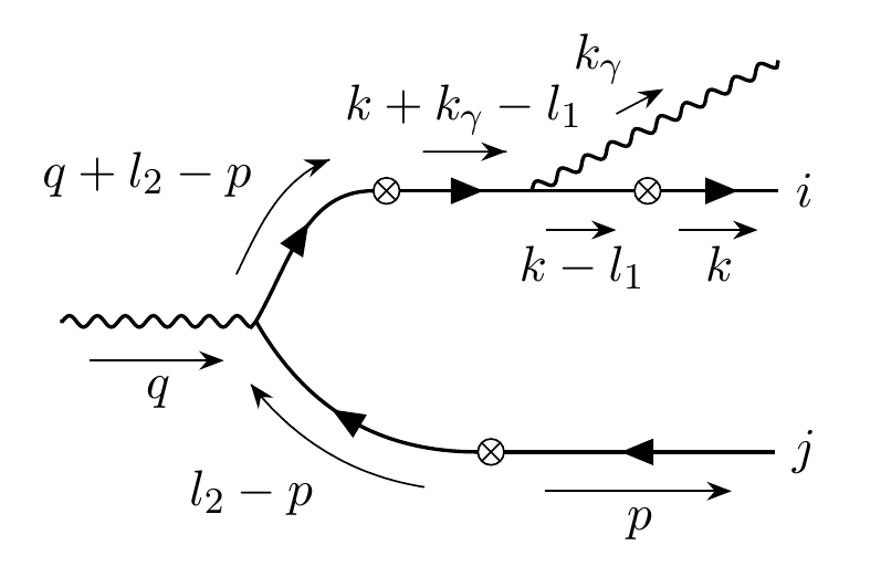
Figure 15: Feynman diagram of the LO contribution to inclusive photon production with all dressed fermion lines. The momenta $l_{1}$ and $l_{2}$ are the momentum kicks from the nucleus to the quark and antiquark respectively.

The amplitude for the hadronic subprocess is given by

$$\mathcal{M}_{\mu\alpha}=-(eq_{f})^{2}\int_{l_{1},l_{2}}\overline{u}(\mathbf{k}) \mathcal{T}_{im}(k-l_{1},k)S_{0}(k-l_{1})\gamma_{\alpha}S_{0}(k+k_{\gamma}-l_{1})\mathcal{T}_{mn}(q+l_{2}-p,k+k_{\gamma}-l_{1})$$

$$\times S_{0}(q+l_{2}-p)\gamma_{\mu}S_{0}(l_{2}-p)\mathcal{T}_{nj}(-p,l_{2}-p)v(\mathbf{p})\enskip,$$ (136)

where $\int_{l_{i}}=\int\mathrm{d}^{4}l_{i}/(2\pi)^{4},i=1,2$ and $\mathcal{T}$ is given by Eq. 83.

Integrating out $l_{1}^{-}$ and $l_{2}^{-}$ using the delta functions embedded in the vertex factors, we are left with the delta function $\delta(q^{-}-P^{-})$ representing the overall longitudinal momentum conservation and integrations over transverse spatial and momentum coordinates. However the quantity of interest is the integral over $l_{1}^{+}$ and $l_{2}^{+}$ given by

$$\mathcal{I}=\int\mathrm{d}l_{1}^{+}\int\mathrm{d}l_{2}^{+}\enskip\frac{N}{D}\enskip,$$ (137)

where

$$N=\overline{u}(\mathbf{k})\gamma^{-}(\not{k}-\not{l_{1}}+m)\gamma_{\alpha}(\not{k}+\not{k}_{\gamma}-\not{l_{1}}+m)\gamma^{-}(\not{q}+\not{l_{2}}-\not{p}+m)\gamma_{\mu}(\not{l_{2}}-\not{p}+m)\gamma^{-}v(\mathbf{p})\enskip,$$ (138)

and

$$D =\Bigg{(}k^{+}-l_{1}^{+}-\frac{M^{2}(\mathbf{k}_{\perp}-\mathbf{l}_{1\perp})}{2k^{-}}+\frac{i\varepsilon}{2k^{-}}\Bigg{)}\Bigg{(}k^{+}+k^{+}_{\gamma}-l_{1}^{+}-\frac{M^{2}(\mathbf{k}_{\perp}+\mathbf{k}_{\gamma\perp}-\mathbf{l}_{1\perp})}{2(k^{-}+k_{\gamma}^{-})}+\frac{i\varepsilon}{2(k^{-}+k_{\gamma}^{-})}\Bigg{)}$$

$$\times\Bigg{(}q^{+}+l_{2}^{+}-p^{+}-\frac{M^{2}(\mathbf{l}_{1\perp}-\mathbf{p}_{\perp})}{2(k^{-}+k_{\gamma}^{-})}+\frac{i\varepsilon}{2(k^{-}+k^{-}_{\gamma})}\Bigg{)}\Bigg{(}l_{2}^{+}-p^{+}+\frac{M^{2}(\mathbf{l}_{1\perp}-\mathbf{p}_{\perp})}{2p^{-}}-\frac{i\varepsilon}{2p^{-}}\Bigg{)}\enskip,$$ (139)

denote the numerator and denominator respectively. Examining the structure of the poles in the propagator terms of the denominator, there are two $l_{1}^{+}$ poles on the positive side of the real axis and independently, two $l_{2}^{+}$ poles on either side of the real axis. Using the property $(\gamma^{-})^{2}=0$, it is easy to see that the numerator does not contain any term proportional to $l_{1}^{+}$ or $l_{2}^{+}$. Therefore the contour for the integration over $l_{1}^{+}$ can be closed below the real axis thereby giving a null result.

The arguments presented thus far does not invoke the possibility of “no scattering” in our definition of the effective vertices or equivalently the $\tilde{U}=\mathds{1}$ case. It can be shown easily that for either $\tilde{U}_{im}=\delta_{im}$ or $\tilde{U}_{mn}=\delta_{mn}$ in the vertex factors appearing in Eq. 136, we will get a nonzero result from the above contour integration. Under these conditions, the two factors appearing in the first line of Eq. 139 resemble energy denominators that appear in light cone perturbation theory (LCPT) Kogut and Soper (1970); Bjorken et al. (1971); Brodsky and Robertson (1995); Brodsky et al. (1998); Venugopalan (1998) and the integration over $l_{2}^{+}$ can be done using the residue theorem. Corresponding to these conditions on the $\tilde{U}$’s, we get the two allowed diagrams with photon emission from the quark line as shown in Fig. 16; these are embedded in our generic diagram Fig. 15.

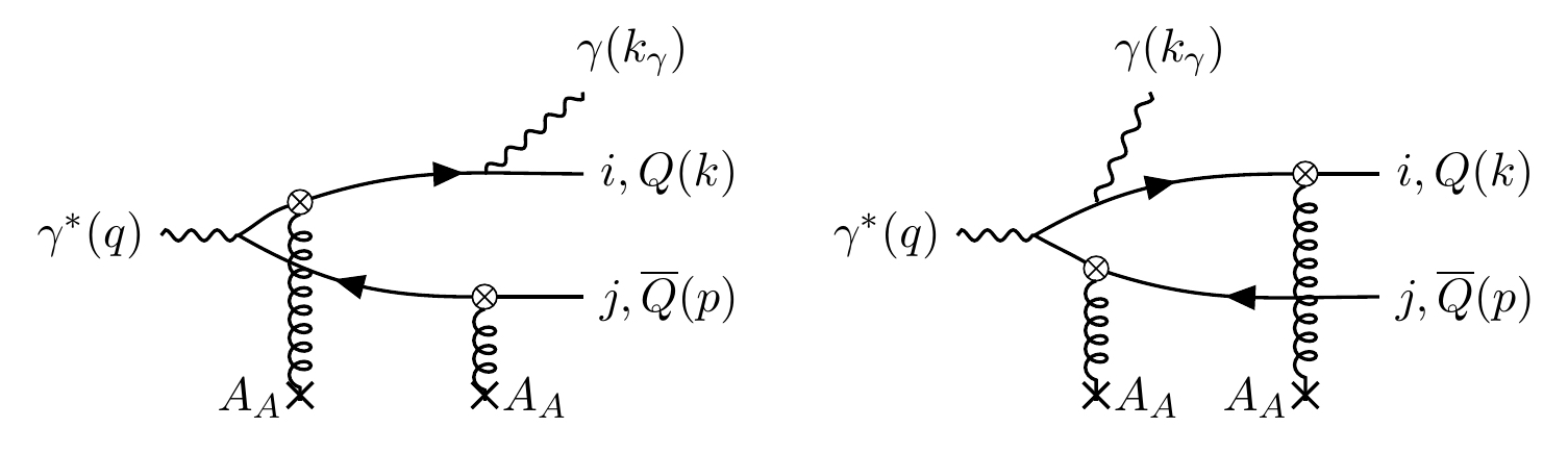
Figure 16: Contributions to the photon production amplitude at LO with photon emission from the quark line. The remaining two diagrams can be obtained by interchanging the quark and antiquark lines.

One can therefore start with the generic case and eventually deduce the impossibility of a secondary scattering subsequent to emission of the photon by an already scattered fermion. This is a consequence of the eikonal approximation in which the nucleus moving at near light speed interacts instantaneously with the quarks thereby removing the possibility of a second scattering. Once the allowed diagrams are computed, we simply need to deduct the contribution in which both quark and antiquark propagate unscattered. The latter have the same magnitude as the allowed diagrams modulo the Wilson line factors. The net contribution is given by Eq. 47.

The same physical principle discussed above for LO also applies to the NLO diagrams which are classified into three broad categories. For the diagrams contributing to the LLx and NLLx JIMWLK evolution, the allowed topologies can be easily extracted from existing literature Balitsky and Chirilli (2013); Kovchegov and Weigert (2007); Balitsky and Chirilli (2008). Since the upper part of these diagrams has the same structure as LO diagrams, the rules discussed in the previous section apply trivially. In the following, we therefore discuss only the genuine $\alpha_{S}$ suppressed contributions in Figs. 5.

We consider one such representative generic diagram (see Fig. 17) which represents real emission of a gluon from the quark or antiquark in addition to the final state photon. We use the line of reasoning made for the LO case to deduce the allowed processes. The amplitude for this subprocess is given by

$$\mathcal{M}_{\mu\alpha;a} =-i(eq_{f})^{2}g\Big{(}\prod_{k=1}^{4}\int_{l_{k}}\Big{)}\enskip\overline{u}(\mathbf{k})\mathcal{T}_{im}(k-l_{1},k)S_{0}(k-l_{1})\gamma_{\alpha}S_{0}(k+k_{\gamma}-l_{1})\mathcal{T}_{mn}(k+k_{\gamma}-l_{1}-l_{2},k+k_{\gamma}-l_{1})$$

$$\times S_{0}(k+k_{\gamma}-l_{1}-l_{2})(t^{b})_{np}\gamma_{\beta}S_{0}(k+k_{\gamma}-l_{1}-l_{2}+l_{3})\mathcal{T}_{pq}(q+l_{4}-p,k+k_{\gamma}-l_{1}-l_{2}+l_{3})$$

$$\times S_{0}(q+l_{4}-p)\gamma_{\mu}\mathcal{T}_{qj}(-p,l_{4}-p)v(\mathbf{p})\times G_{0}^{\beta\nu;bc}(l_{3})\mathcal{T}_{\nu\rho;ca}(l_{3},k_{g}){\epsilon^{\rho}}^{*}(\mathbf{k}_{g})\enskip,$$ (140)

where the vertex factors for the fermion and gluon propagators are given respectively by Eqs. 83 and 108.

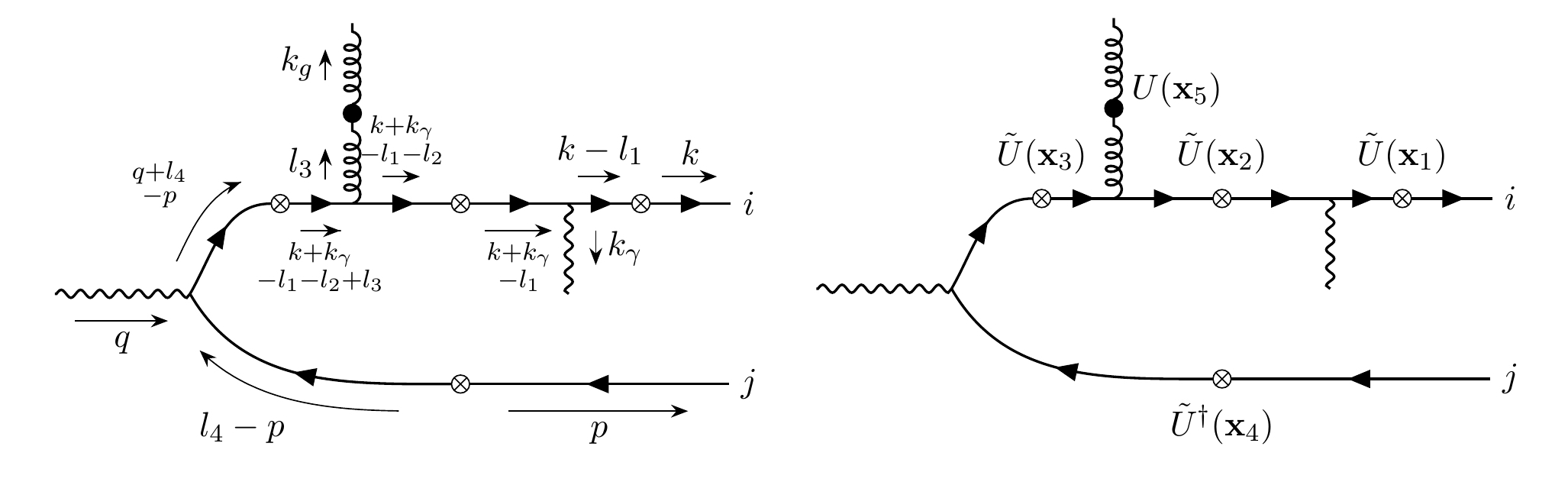
Figure 17: Real emission graph for NLO with all fermion lines dressed. $l_{1}$, $l_{2}$ and $l_{4}$ represent the momentum transfer from the nucleus to the quark and antiquark line at different points in the scattering process. $l_{3}$ is the momentum carried by the gluon prior to scattering off the nucleus. $i$ and $j$ represent fundamental color indices. The Wilson line factors associated with each effective vertex are shown on the right.

By carefully integrating out the $l_{i}^{-}$’s ($i=1,\dots,4$) using the $\delta$-functions, the amplitude can be cast in terms of a momentum conserving delta function $\delta(q^{-}-p^{-}-k^{-}-k^{-}_{\gamma}-k^{-}_{g})$, integrations over transverse spatial and momentum coordinates and the following integral of interest.

$$\mathcal{I}_{1}=\Big{(}\prod_{k=1}^{4}\int\mathrm{d}l_{k}^{+}\Big{)}\enskip\frac{N_{1}}{D_{1}}$$ (141)

where

$$N_{1} =\overline{u}(\mathbf{k})\gamma^{-}[\gamma^{+}k^{-}-\bm{\gamma}_{\perp}.(\mathbf{k}_{\perp}-\mathbf{l}_{1\perp})+m]\gamma_{\alpha}[\gamma^{+}(k^{-}+k^{-}_{\gamma})-\bm{\gamma}_{\perp}.(\mathbf{k}_{\perp}+\mathbf{k}_{\gamma\perp}-\mathbf{l}_{1\perp})+m]\gamma^{-}$$

$$\times[\gamma^{+}(k^{-}+k^{-}_{\gamma})-\bm{\gamma}_{\perp}.(\mathbf{k}_{\perp}+\mathbf{k}_{\gamma\perp}-\mathbf{l}_{1\perp}-\mathbf{l}_{2\perp})+m]\gamma_{\beta}[\gamma^{+}(k^{-}+k^{-}_{\gamma}+k_{g}^{-})-\bm{\gamma}_{\perp}.(\mathbf{k}_{\perp}+\mathbf{k}_{\gamma\perp}-\mathbf{l}_{1\perp}-\mathbf{l}_{2\perp}+\mathbf{l}_{3\perp})+m]$$

$$\times\gamma^{-}[\gamma^{+}(k^{-}+k^{-}_{\gamma}+k_{g}^{-})-\bm{\gamma}_{\perp}.(\mathbf{l}_{4\perp}-\mathbf{p}_{\perp})+m]\gamma_{\mu}[\gamma^{+}p^{-}+\bm{\gamma}_{\perp}.(\mathbf{l}_{4\perp}-\mathbf{p}_{\perp})-m]\gamma^{-}\Bigg{(}-{\epsilon^{\beta}}^{*}(\mathbf{k}_{g})+\frac{(l_{3}.\epsilon^{*}(\mathbf{k}_{g}))n^{\beta}}{k^{-}_{g}}\Bigg{)}\enskip,$$ (142)

is obtained using $n.\epsilon^{*}(\mathbf{k}_{g})=0$ and $(\gamma^{-})^{2}=0$ and

$$D_{1} =\Bigg{(}k^{+}-l_{1}^{+}-\frac{M^{2}(\mathbf{k}_{\perp}-\mathbf{l}_{1\perp})}{2k^{-}}+\frac{i\varepsilon}{2k^{-}}\Bigg{)}\Bigg{(}k^{+}+k_{\gamma}^{+}-l_{1}^{+}-\frac{M^{2}(\mathbf{k}_{\perp}+\mathbf{k}_{\gamma\perp}-\mathbf{l}_{1\perp})}{2(k^{-}+k^{-}_{\gamma})}+\frac{i\varepsilon}{2(k^{-}+k^{-}_{\gamma})}\Bigg{)}$$

$$\times\Bigg{(}k^{+}+k^{+}_{\gamma}-l_{1}^{+}-l^{+}_{2}-\frac{M^{2}(\mathbf{k}_{\perp}+\mathbf{k}_{\gamma\perp}-\mathbf{l}_{1\perp}-\mathbf{l}_{2\perp})}{2(k^{-}+k^{-}_{\gamma})}+\frac{i\varepsilon}{2(k^{-}+k^{-}_{\gamma})}\Bigg{)}\Bigg{(}l^{+}_{3}-\frac{\mathbf{l}_{3\perp}^{2}}{2k^{-}_{g}}+\frac{i\varepsilon}{2k^{-}_{g}}\Bigg{)}$$

$$\times\Bigg{(}k^{+}+k^{+}_{\gamma}-l_{1}^{+}-l^{+}_{2}+l_{3}^{+}-\frac{M^{2}(\mathbf{k}_{\perp}+\mathbf{k}_{\gamma\perp}-\mathbf{l}_{1\perp}-\mathbf{l}_{2\perp}+\mathbf{l}_{3\perp})}{2(k^{-}+k^{-}_{\gamma}+k^{-}_{g})}+\frac{i\varepsilon}{2(k^{-}+k^{-}_{\gamma}+k^{-}_{g})}\Bigg{)}$$

$$\times\Bigg{(}q^{+}+l^{+}_{4}-p^{+}-\frac{M^{2}(\mathbf{l}_{4\perp}-\mathbf{p}_{\perp})}{2(k^{-}+k^{-}_{\gamma}+k^{-}_{g})}+\frac{i\varepsilon}{2(k^{-}+k^{-}_{\gamma}+k^{-}_{g})}\Bigg{)}\Bigg{(}l^{+}_{4}-p^{+}+\frac{M^{2}(\mathbf{l}_{4\perp}-\mathbf{p}_{\perp})}{2p^{-}}-\frac{i\varepsilon}{2p^{-}}\Bigg{)}\enskip.$$ (143)

The expressions above clearly demonstrate that the numerator doesn’t have any term proportional to $l_{1}^{+}$, $l_{2}^{+}$ or $l_{3}^{+}$ and the poles for all these variables are on the same side of the real axis. Hence the integration contours for any such variable can be deformed in a way so as not to enclose any pole giving a result of zero for general $U$ and $\tilde{U}$’s depicted in Fig. 17. However it can be easily shown that for the following three cases

• $\tilde{U}(\mathbf{x}_{1})=\tilde{U}(\mathbf{x}_{3})=\mathds{1}$ with rest of the Wilson lines being general (including the identity matrix),

• $\tilde{U}(\mathbf{x}_{2})=\tilde{U}(\mathbf{x}_{3})=\mathds{1}$ with rest of the Wilson lines being general and

• $\tilde{U}(\mathbf{x}_{1})=\tilde{U}(\mathbf{x}_{2})=\mathds{1}$, $U(\mathbf{x}_{5})=\mathds{1}$ and remaining two being general,

we get a finite result. Diagrammatically, this corresponds to the processes shown respectively in Fig. 18 or equivalently the diagrams in Fig. 19 in the “shock wave” approach. Similar arguments can be applied to find the allowed virtual graphs at NLO.

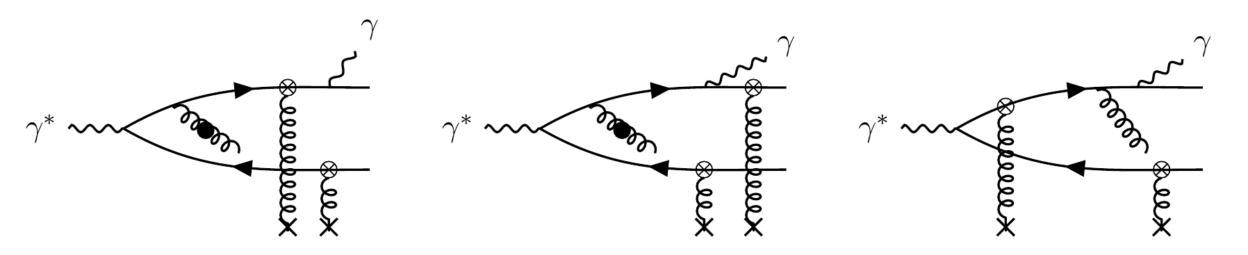
Figure 18: The allowed set of diagrams embedded in Fig. 17.

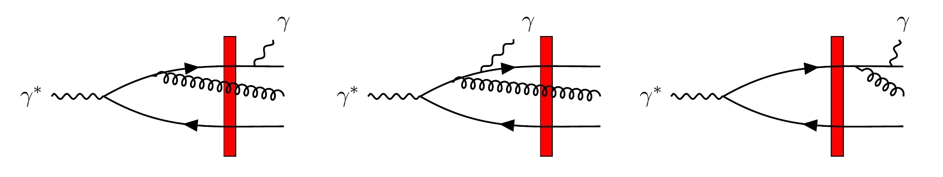
Figure 19: An equivalent depiction of the allowed set of diagrams embedded in Fig. 17 with the Lorentz contracted nucleus shown here by the red rectangular wall.

References

- Breitweg et al. (2000) J. Breitweg et al. (ZEUS), “Measurement of inclusive prompt photon photoproduction at HERA,” Phys. Lett. B472, 175–188 (2000), arXiv:hep-ex/9910045 [hep-ex] .
- Aktas et al. (2005) A. Aktas et al. (H1), “Measurement of prompt photon cross sections in photoproduction at HERA,” Eur. Phys. J. C38, 437–445 (2005), arXiv:hep-ex/0407018 [hep-ex] .
- Chekanov et al. (2007) S. Chekanov et al. (ZEUS), “Measurement of prompt photons with associated jets in photoproduction at HERA,” Eur. Phys. J. C49, 511–522 (2007), arXiv:hep-ex/0608028 [hep-ex] .
- Chekanov et al. (2004) S. Chekanov et al. (ZEUS), “Observation of isolated high E(T) photons in deep inelastic scattering,” Phys. Lett. B595, 86–100 (2004), arXiv:hep-ex/0402019 [hep-ex] .
- Aaron et al. (2008) F. D. Aaron et al. (H1), “Measurement of isolated photon production in deep-inelastic scattering at HERA,” Eur. Phys. J. C54, 371–387 (2008), arXiv:0711.4578 [hep-ex] .
- Chekanov et al. (2010) S. Chekanov et al. (ZEUS), “Measurement of isolated photon production in deep inelastic ep scattering,” Phys. Lett. B687, 16–25 (2010), arXiv:0909.4223 [hep-ex] .
- Abramowicz et al. (2012) H. Abramowicz et al. (ZEUS), “Measurement of isolated photons accompanied by jets in deep inelastic scattering,” Phys. Lett. B715, 88–97 (2012), arXiv:1206.2270 [hep-ex] .
- Gehrmann-De Ridder et al. (2006) A. Gehrmann-De Ridder, T. Gehrmann, and E. Poulsen, “Isolated photons in deep inelastic scattering,” Phys. Rev. Lett. 96, 132002 (2006), arXiv:hep-ph/0601073 [hep-ph] .
- Schmidt et al. (2016) Carl Schmidt, Jon Pumplin, Daniel Stump, and C. P. Yuan, “CT14QED parton distribution functions from isolated photon production in deep inelastic scattering,” Phys. Rev. D93, 114015 (2016), arXiv:1509.02905 [hep-ph] .
- Gribov et al. (1983) L. V. Gribov, E. M. Levin, and M. G. Ryskin, “Semihard Processes in QCD,” Phys. Rept. 100, 1–150 (1983).
- Mueller and Qiu (1986) Alfred H. Mueller and Jian-wei Qiu, “Gluon Recombination and Shadowing at Small Values of ,” Nucl. Phys. B268, 427–452 (1986).
- McLerran and Venugopalan (1994a) Larry D. McLerran and Raju Venugopalan, “Computing quark and gluon distribution functions for very large nuclei,” Phys. Rev. D49, 2233–2241 (1994a), arXiv:hep-ph/9309289 [hep-ph] .
- McLerran and Venugopalan (1994b) Larry D. McLerran and Raju Venugopalan, “Gluon distribution functions for very large nuclei at small transverse momentum,” Phys. Rev. D49, 3352–3355 (1994b), arXiv:hep-ph/9311205 [hep-ph] .
- McLerran and Venugopalan (1994c) Larry D. McLerran and Raju Venugopalan, “Green’s functions in the color field of a large nucleus,” Phys. Rev. D50, 2225–2233 (1994c), arXiv:hep-ph/9402335 [hep-ph] .
- Iancu and Venugopalan (2003) Edmond Iancu and Raju Venugopalan, “The Color glass condensate and high-energy scattering in QCD,” in In *Hwa, R.C. (ed.) et al.: Quark gluon plasma* 249-3363 (2003) arXiv:hep-ph/0303204 [hep-ph] .
- Gelis et al. (2010) Francois Gelis, Edmond Iancu, Jamal Jalilian-Marian, and Raju Venugopalan, “The Color Glass Condensate,” Ann. Rev. Nucl. Part. Sci. 60, 463–489 (2010), arXiv:1002.0333 [hep-ph] .
- Kovchegov and Levin (2012) Yuri V. Kovchegov and Eugene Levin, Quantum chromodynamics at high energy, Vol. 33 (Cambridge University Press, 2012).
- Blaizot (2017) Jean-Paul Blaizot, “High gluon densities in heavy ion collisions,” Rept. Prog. Phys. 80, 032301 (2017), arXiv:1607.04448 [hep-ph] .
- Fubini and Furlan (1965) S. Fubini and G. Furlan, “Renormalization effects for partially conserved currents,” Physics 1, 229–247 (1965).
- Bardakci and Halpern (1968) K. Bardakci and M. B. Halpern, “Theories at infinite momentum,” Phys. Rev. 176, 1686–1699 (1968).
- Weinberg (1966) Steven Weinberg, “Dynamics at infinite momentum,” Phys. Rev. 150, 1313–1318 (1966).
- Susskind (1968) Leonard Susskind, “Model of selfinduced strong interactions,” Phys. Rev. 165, 1535–1546 (1968).
- Jeon and Venugopalan (2004) Sangyong Jeon and Raju Venugopalan, “Random walks of partons in SU(N(c)) and classical representations of color charges in QCD at small x,” Phys. Rev. D70, 105012 (2004), arXiv:hep-ph/0406169 [hep-ph] .
- Jalilian-Marian et al. (1997) Jamal Jalilian-Marian, Alex Kovner, Andrei Leonidov, and Heribert Weigert, “The BFKL equation from the Wilson renormalization group,” Nucl. Phys. B504, 415–431 (1997), arXiv:hep-ph/9701284 [hep-ph] .
- Jalilian-Marian et al. (1998) Jamal Jalilian-Marian, Alex Kovner, and Heribert Weigert, “The Wilson renormalization group for low physics: Gluon evolution at finite parton density,” Phys. Rev. D59, 014015 (1998), arXiv:hep-ph/9709432 [hep-ph] .
- Iancu et al. (2001a) Edmond Iancu, Andrei Leonidov, and Larry D. McLerran, “The Renormalization group equation for the color glass condensate,” Phys. Lett. B510, 133–144 (2001a), arXiv:hep-ph/0102009 [hep-ph] .
- Iancu et al. (2001b) Edmond Iancu, Andrei Leonidov, and Larry D. McLerran, “Nonlinear gluon evolution in the color glass condensate. 1.” Nucl. Phys. A692, 583–645 (2001b), arXiv:hep-ph/0011241 [hep-ph] .
- Ferreiro et al. (2002) Elena Ferreiro, Edmond Iancu, Andrei Leonidov, and Larry McLerran, “Nonlinear gluon evolution in the color glass condensate. 2.” Nucl. Phys. A703, 489–538 (2002), arXiv:hep-ph/0109115 [hep-ph] .
- Weigert (2005) Heribert Weigert, “Evolution at small x(bj): The Color glass condensate,” Prog. Part. Nucl. Phys. 55, 461–565 (2005), arXiv:hep-ph/0501087 [hep-ph] .
- Balitsky (1996) I. Balitsky, “Operator expansion for high-energy scattering,” Nucl. Phys. B463, 99–160 (1996), arXiv:hep-ph/9509348 [hep-ph] .
- Weigert (2002) Heribert Weigert, “Unitarity at small Bjorken x,” Nucl. Phys. A703, 823–860 (2002), arXiv:hep-ph/0004044 [hep-ph] .
- Kovchegov (1999) Yuri V. Kovchegov, “Small F(2) structure function of a nucleus including multiple pomeron exchanges,” Phys. Rev. D60, 034008 (1999), arXiv:hep-ph/9901281 [hep-ph] .
- Rummukainen and Weigert (2004) Kari Rummukainen and Heribert Weigert, “Universal features of JIMWLK and BK evolution at small ,” Nucl. Phys. A739, 183–226 (2004), arXiv:hep-ph/0309306 [hep-ph] .
- Dumitru et al. (2011) Adrian Dumitru, Jamal Jalilian-Marian, Tuomas Lappi, Bjoern Schenke, and Raju Venugopalan, “Renormalization group evolution of multi-gluon correlators in high energy QCD,” Phys. Lett. B706, 219–224 (2011), arXiv:1108.4764 [hep-ph] .
- Benic et al. (2017) Sanjin Benic, Kenji Fukushima, Oscar Garcia-Montero, and Raju Venugopalan, “Probing gluon saturation with next-to-leading order photon production at central rapidities in proton-nucleus collisions,” JHEP 01, 115 (2017), arXiv:1609.09424 [hep-ph] .
- Gelis and Jalilian-Marian (2002) Francois Gelis and Jamal Jalilian-Marian, “Photon production in high-energy proton nucleus collisions,” Phys. Rev. D66, 014021 (2002), arXiv:hep-ph/0205037 [hep-ph] .
- Dominguez et al. (2011) Fabio Dominguez, Cyrille Marquet, Bo-Wen Xiao, and Feng Yuan, “Universality of Unintegrated Gluon Distributions at small ,” Phys. Rev. D83, 105005 (2011), arXiv:1101.0715 [hep-ph] .
- Gribov et al. (1966) V. N. Gribov, B. L. Ioffe, and I. Ya. Pomeranchuk, “What is the range of interactions at high-energies,” Sov. J. Nucl. Phys. 2, 549 (1966), [Yad. Fiz.2,768(1965)].
- Ioffe (1969) B. L. Ioffe, “Space-time picture of photon and neutrino scattering and electroproduction cross-section asymptotics,” Phys. Lett. 30B, 123–125 (1969).
- Bjorken et al. (1971) J. D. Bjorken, John B. Kogut, and Davison E. Soper, “Quantum Electrodynamics at Infinite Momentum: Scattering from an External Field,” Phys. Rev. D3, 1382 (1971).
- Nikolaev and Zakharov (1991) Nikolai N. Nikolaev and B. G. Zakharov, “Color transparency and scaling properties of nuclear shadowing in deep inelastic scattering,” Z. Phys. C49, 607–618 (1991).
- Benic and Fukushima (2017) Sanjin Benic and Kenji Fukushima, “Photon from the annihilation process with CGC in the collision,” Nucl. Phys. A958, 1–24 (2017), arXiv:1602.01989 [hep-ph] .
- Altinoluk et al. (2018) Tolga Altinoluk, Néstor Armesto, Alex Kovner, Michael Lublinsky, and Elena Petreska, “Soft photon and two hard jets forward production in proton-nucleus collisions,” (2018), arXiv:1802.01398 [hep-ph] .
- Dokshitzer (1977) Yuri L. Dokshitzer, “Calculation of the Structure Functions for Deep Inelastic Scattering and e+ e- Annihilation by Perturbation Theory in Quantum Chromodynamics.” Sov. Phys. JETP 46, 641–653 (1977), [Zh. Eksp. Teor. Fiz.73,1216(1977)].
- Gribov and Lipatov (1972) V. N. Gribov and L. N. Lipatov, “Deep inelastic e p scattering in perturbation theory,” Sov. J. Nucl. Phys. 15, 438–450 (1972), [Yad. Fiz.15,781(1972)].
- Altarelli and Parisi (1977) Guido Altarelli and G. Parisi, “Asymptotic Freedom in Parton Language,” Nucl. Phys. B126, 298–318 (1977).
- Abe et al. (1993) I. Abe et al. (H1), “Measurement of the proton structure function F2 in the low region at HERA,” Nucl. Phys. B407, 515–538 (1993).
- Ahmed et al. (1995) T. Ahmed et al. (H1), “A Measurement of the proton structure function ,” Nucl. Phys. B439, 471–502 (1995), arXiv:hep-ex/9503001 [hep-ex] .
- Derrick et al. (1993) M. Derrick et al. (ZEUS), “Measurement of the proton structure function F2 in ep scattering at HERA,” Phys. Lett. B316, 412–426 (1993).
- Derrick et al. (1995) M. Derrick et al. (ZEUS), “Measurement of the proton structure function F2 from the 1993 HERA data,” Z. Phys. C65, 379–398 (1995).
- Martin et al. (1994) Alan D. Martin, W. James Stirling, and R. G. Roberts, “Parton distributions of the proton,” Phys. Rev. D50, 6734–6752 (1994), arXiv:hep-ph/9406315 [hep-ph] .
- Lai et al. (1995) H. L. Lai, J. Botts, J. Huston, J. G. Morfin, J. F. Owens, Jian-wei Qiu, W. K. Tung, and H. Weerts, “Global QCD analysis and the CTEQ parton distributions,” Phys. Rev. D51, 4763–4782 (1995), arXiv:hep-ph/9410404 [hep-ph] .
- Gelis and Venugopalan (2006a) Francois Gelis and Raju Venugopalan, “Particle production in field theories coupled to strong external sources,” Nucl. Phys. A776, 135–171 (2006a), arXiv:hep-ph/0601209 [hep-ph] .
- Gelis and Venugopalan (2006b) Francois Gelis and Raju Venugopalan, “Particle production in field theories coupled to strong external sources. II. Generating functions,” Nucl. Phys. A779, 177–196 (2006b), arXiv:hep-ph/0605246 [hep-ph] .
- Gelis et al. (2007) Francois Gelis, Tuomas Lappi, and Raju Venugopalan, “High energy scattering in Quantum Chromodynamics,” Hadron physics. Proceedings, 10th International Workshop, Florianopolis, Brazil, April 26-31, 2007, Int. J. Mod. Phys. E16, 2595–2637 (2007), arXiv:0708.0047 [hep-ph] .
- Gelis et al. (2008a) Francois Gelis, Tuomas Lappi, and Raju Venugopalan, “High energy factorization in nucleus-nucleus collisions,” Phys. Rev. D78, 054019 (2008a), arXiv:0804.2630 [hep-ph] .
- Gelis et al. (2008b) Francois Gelis, Tuomas Lappi, and Raju Venugopalan, “High energy factorization in nucleus-nucleus collisions. II. Multigluon correlations,” Phys. Rev. D78, 054020 (2008b), arXiv:0807.1306 [hep-ph] .
- Balitsky and Chirilli (2013) Ian Balitsky and Giovanni A. Chirilli, “Rapidity evolution of Wilson lines at the next-to-leading order,” Phys. Rev. D88, 111501 (2013), arXiv:1309.7644 [hep-ph] .
- Grabovsky (2013) A. V. Grabovsky, “Connected contribution to the kernel of the evolution equation for 3-quark Wilson loop operator,” JHEP 09, 141 (2013), arXiv:1307.5414 [hep-ph] .
- Kovner et al. (2014) Alex Kovner, Michael Lublinsky, and Yair Mulian, “Jalilian-Marian, Iancu, McLerran, Weigert, Leonidov, Kovner evolution at next to leading order,” Phys. Rev. D89, 061704 (2014), arXiv:1310.0378 [hep-ph] .
- Kovchegov and Weigert (2007) Yuri V. Kovchegov and Heribert Weigert, “Triumvirate of Running Couplings in Small-x Evolution,” Nucl. Phys. A784, 188–226 (2007), arXiv:hep-ph/0609090 [hep-ph] .
- Balitsky and Chirilli (2008) Ian Balitsky and Giovanni A. Chirilli, “Next-to-leading order evolution of color dipoles,” Phys. Rev. D77, 014019 (2008), arXiv:0710.4330 [hep-ph] .
- Balitsky (2007) Ian Balitsky, “Quark contribution to the small-x evolution of color dipole,” Phys. Rev. D75, 014001 (2007), arXiv:hep-ph/0609105 [hep-ph] .
- Low (1958) F. E. Low, “Bremsstrahlung of very low-energy quanta in elementary particle collisions,” Phys. Rev. 110, 974–977 (1958).
- Burnett and Kroll (1968) T. H. Burnett and Norman M. Kroll, “Extension of the low soft photon theorem,” Phys. Rev. Lett. 20, 86 (1968).
- Bell and Van Royen (1969) J. S. Bell and R. Van Royen, “On the low-burnett-kroll theorem for soft-photon emission,” Nuovo Cim. A60, 62–68 (1969).
- McLerran and Venugopalan (1999) Larry D. McLerran and Raju Venugopalan, “Fock space distributions, structure functions, higher twists and small ,” Phys. Rev. D59, 094002 (1999), arXiv:hep-ph/9809427 [hep-ph] .
- Peskin and Schroeder (1995) Michael E. Peskin and Daniel V. Schroeder, An Introduction to quantum field theory (Addison-Wesley, Reading, USA, 1995).
- Blaizot et al. (2004a) Jean Paul Blaizot, Francois Gelis, and Raju Venugopalan, “High-energy pA collisions in the color glass condensate approach. 1. Gluon production and the Cronin effect,” Nucl. Phys. A743, 13–56 (2004a), arXiv:hep-ph/0402256 [hep-ph] .
- Jalilian-Marian and Kovchegov (2006) Jamal Jalilian-Marian and Yuri V. Kovchegov, “Saturation physics and deuteron-Gold collisions at RHIC,” Prog. Part. Nucl. Phys. 56, 104–231 (2006), arXiv:hep-ph/0505052 [hep-ph] .
- Fujii et al. (2006) Hirotsugu Fujii, Francois Gelis, and Raju Venugopalan, “Quark pair production in high energy pA collisions: General features,” Nucl. Phys. A780, 146–174 (2006), arXiv:hep-ph/0603099 [hep-ph] .
- Kuraev et al. (1977) E. A. Kuraev, L. N. Lipatov, and Victor S. Fadin, “The Pomeranchuk Singularity in Nonabelian Gauge Theories,” Sov. Phys. JETP 45, 199–204 (1977), [Zh. Eksp. Teor. Fiz.72,377(1977)].
- Balitsky and Lipatov (1978) I. I. Balitsky and L. N. Lipatov, “The Pomeranchuk Singularity in Quantum Chromodynamics,” Sov. J. Nucl. Phys. 28, 822–829 (1978), [Yad. Fiz.28,1597(1978)].
- Gelis and Venugopalan (2004) Francois Gelis and Raju Venugopalan, “Large mass q production from the color glass condensate,” Phys. Rev. D69, 014019 (2004), arXiv:hep-ph/0310090 [hep-ph] .
- Aurenche et al. (1984) P. Aurenche, A. Douiri, R. Baier, M. Fontannaz, and D. Schiff, “The Deep Compton Scattering: Single Photon Spectrum and Photon - Hadron Correlations Beyond Leading Logarithms,” Z. Phys. C24, 309 (1984).
- Gehrmann-De Ridder et al. (2000) A. Gehrmann-De Ridder, G. Kramer, and H. Spiesberger, “Photon plus jet-cross sections in deep inelastic e p collisions at order O(alpha**2 alpha(s)),” Nucl. Phys. B578, 326–350 (2000), arXiv:hep-ph/0003082 [hep-ph] .
- Kramer et al. (1998) G. Kramer, D. Michelsen, and H. Spiesberger, “Production of hard photons and jets in deep inelastic lepton proton scattering at order O (alpha-s),” Eur. Phys. J. C5, 293–301 (1998), arXiv:hep-ph/9712309 [hep-ph] .
- Michelsen (1995) Dirk Michelsen, Radiative corrections of order alpha-s for production of hard photons by HERA, Ph.D. thesis, Hamburg U. (1995).
- Gelis and Jalilian-Marian (2003) Francois Gelis and Jamal Jalilian-Marian, “From DIS to proton nucleus collisions in the color glass condensate model,” Phys. Rev. D67, 074019 (2003), arXiv:hep-ph/0211363 [hep-ph] .
- Dominguez et al. (2012) Fabio Dominguez, Jian-Wei Qiu, Bo-Wen Xiao, and Feng Yuan, “On the linearly polarized gluon distributions in the color dipole model,” Phys. Rev. D85, 045003 (2012), arXiv:1109.6293 [hep-ph] .
- Kovchegov and Mueller (1998) Yuri V. Kovchegov and Alfred H. Mueller, “Gluon production in current nucleus and nucleon - nucleus collisions in a quasiclassical approximation,” Nucl. Phys. B529, 451–479 (1998), arXiv:hep-ph/9802440 [hep-ph] .
- Diehl (2003) M. Diehl, “Generalized parton distributions,” Phys. Rept. 388, 41–277 (2003), arXiv:hep-ph/0307382 [hep-ph] .
- Kogut and Soper (1970) John B. Kogut and Davison E. Soper, “Quantum Electrodynamics in the Infinite Momentum Frame,” Phys. Rev. D1, 2901–2913 (1970).
- Brodsky and Robertson (1995) Stanley J. Brodsky and David G. Robertson, “Light cone quantization and QCD phenomenology,” in Confinement physics. Proceedings, 1st ELFE Summer School, Cambridge, UK, July 22-28, 1995 (1995) pp. 71–110, arXiv:hep-ph/9511374 [hep-ph] .
- Brodsky et al. (1998) Stanley J. Brodsky, Hans-Christian Pauli, and Stephen S. Pinsky, “Quantum chromodynamics and other field theories on the light cone,” Phys. Rept. 301, 299–486 (1998), arXiv:hep-ph/9705477 [hep-ph] .
- Venugopalan (1998) Raju Venugopalan, “Introduction to light cone field theory and high-energy scattering,” Hadrons in dense matter and hadrosynthesis. Proceedings, 11th Chris Engelbrecht Summer School, Cape Town, South Africa, February 4-13, 1998, (1998), 10.1007/BFb0107312, [Lect. Notes Phys.516,89(1999)], arXiv:nucl-th/9808023 [nucl-th] .
- Venugopalan (1999) Raju Venugopalan, “Classical methods in DIS and nuclear scattering at small ,” Strong interactions at low and high-energies. Proceedings, 39th Cracow School of Theoretical Physics, Zakopane, Poland, May 29-June 8, 1999, Acta Phys. Polon. B30, 3731–3761 (1999), arXiv:hep-ph/9911371 [hep-ph] .
- Ayala et al. (1995) Alejandro Ayala, Jamal Jalilian-Marian, Larry D. McLerran, and Raju Venugopalan, “The Gluon propagator in nonAbelian Weizsäcker-Williams fields,” Phys. Rev. D52, 2935–2943 (1995), arXiv:hep-ph/9501324 [hep-ph] .
- Ayala et al. (1996) Alejandro Ayala, Jamal Jalilian-Marian, Larry D. McLerran, and Raju Venugopalan, “Quantum corrections to the Weizsacker-Williams gluon distribution function at small x,” Phys. Rev. D53, 458–475 (1996), arXiv:hep-ph/9508302 [hep-ph] .
- Gelis and Mehtar-Tani (2006) Francois Gelis and Yacine Mehtar-Tani, “Gluon propagation inside a high-energy nucleus,” Phys. Rev. D73, 034019 (2006), arXiv:hep-ph/0512079 [hep-ph] .
- Blaizot et al. (2004b) Jean Paul Blaizot, Francois Gelis, and Raju Venugopalan, “High-energy pA collisions in the color glass condensate approach. 2. Quark production,” Nucl. Phys. A743, 57–91 (2004b), arXiv:hep-ph/0402257 [hep-ph] .
- Balitsky and Belitsky (2002) I. I. Balitsky and Andrei V. Belitsky, “Nonlinear evolution in high density QCD,” Nucl. Phys. B629, 290–322 (2002), arXiv:hep-ph/0110158 [hep-ph] .
- Hebecker and Weigert (1998) Arthur Hebecker and H. Weigert, “Small x parton distributions of large hadronic targets,” Phys. Lett. B432, 215–221 (1998), arXiv:hep-ph/9804217 [hep-ph] .
- Kovchegov and Tuchin (2002) Yuri V. Kovchegov and Kirill Tuchin, “Inclusive gluon production in DIS at high parton density,” Phys. Rev. D65, 074026 (2002), arXiv:hep-ph/0111362 [hep-ph] .
- (95) Kaushik Roy and Raju Venugopalan, in preparation .
- Bartels et al. (2001) Jochen Bartels, S. Gieseke, and C. F. Qiao, “The Reggeon vertex in next-to-leading order QCD,” Phys. Rev. D63, 056014 (2001), [Erratum: Phys. Rev.D65,079902(2002)], arXiv:hep-ph/0009102 [hep-ph] .
- Bartels et al. (2002a) J. Bartels, D. Colferai, S. Gieseke, and A. Kyrieleis, “NLO corrections to the photon impact factor: Combining real and virtual corrections,” Phys. Rev. D66, 094017 (2002a), arXiv:hep-ph/0208130 [hep-ph] .
- Bartels et al. (2002b) Jochen Bartels, S. Gieseke, and A. Kyrieleis, “The Process : Real corrections to the virtual photon impact factor,” Phys. Rev. D65, 014006 (2002b), arXiv:hep-ph/0107152 [hep-ph] .
- Balitsky and Chirilli (2011) Ian Balitsky and Giovanni A. Chirilli, “Photon impact factor in the next-to-leading order,” Phys. Rev. D83, 031502 (2011), arXiv:1009.4729 [hep-ph] .
- Beuf (2012) Guillaume Beuf, “NLO corrections for the dipole factorization of DIS structure functions at low ,” Phys. Rev. D85, 034039 (2012), arXiv:1112.4501 [hep-ph] .
- Beuf (2016) Guillaume Beuf, “Dipole factorization for DIS at NLO: Loop correction to the light-front wave functions,” Phys. Rev. D94, 054016 (2016), arXiv:1606.00777 [hep-ph] .
- Beuf (2017) Guillaume Beuf, “Dipole factorization for DIS at NLO: Combining the and contributions,” Phys. Rev. D96, 074033 (2017), arXiv:1708.06557 [hep-ph] .
- Hanninen et al. (2017) H. Hanninen, T. Lappi, and R. Paatelainen, “One-loop corrections to light cone wave functions: the dipole picture DIS cross section,” (2017), arXiv:1711.08207 [hep-ph] .
- Ducloue et al. (2017a) B. Ducloue, H. Hanninen, T. Lappi, and Y. Zhu, “Deep inelastic scattering in the dipole picture at next-to-leading order,” Phys. Rev. D96, 094017 (2017a), arXiv:1708.07328 [hep-ph] .
- Kovchegov and Weigert (2008) Yuri V. Kovchegov and Heribert Weigert, “Collinear Singularities and Running Coupling Corrections to Gluon Production in CGC,” Nucl. Phys. A807, 158–189 (2008), arXiv:0712.3732 [hep-ph] .
- Ducloue et al. (2017b) B. Ducloue, E. Iancu, T. Lappi, A. H. Mueller, G. Soyez, D. N. Triantafyllopoulos, and Y. Zhu, “On the use of a running coupling in the NLO calculation of forward hadron production,” (2017b), arXiv:1712.07480 [hep-ph] .
- Accardi et al. (2016) A. Accardi et al., “Electron Ion Collider: The Next QCD Frontier,” Eur. Phys. J. A52, 268 (2016), arXiv:1212.1701 [nucl-ex] .
- Aschenauer et al. (2017) E. C. Aschenauer, S. Fazio, J. H. Lee, H. Mantysaari, B. S. Page, B. Schenke, T. Ullrich, R. Venugopalan, and P. Zurita, “The Electron-Ion Collider: Assessing the Energy Dependence of Key Measurements,” (2017), arXiv:1708.01527 [nucl-ex] .
- Boussarie et al. (2014) R. Boussarie, A. V. Grabovsky, L. Szymanowski, and S. Wallon, “Impact factor for high-energy two and three jets diffractive production,” JHEP 09, 026 (2014), arXiv:1405.7676 [hep-ph] .
- Boussarie et al. (2016) R. Boussarie, A. V. Grabovsky, L. Szymanowski, and S. Wallon, “On the one loop impact factor and the exclusive diffractive cross sections for the production of two or three jets,” JHEP 11, 149 (2016), arXiv:1606.00419 [hep-ph] .
- Boussarie et al. (2017) R. Boussarie, A. V. Grabovsky, D. Yu. Ivanov, L. Szymanowski, and S. Wallon, “Next-to-Leading Order Computation of Exclusive Diffractive Light Vector Meson Production in a Saturation Framework,” Phys. Rev. Lett. 119, 072002 (2017), arXiv:1612.08026 [hep-ph] .
- Chirilli et al. (2012a) Giovanni A. Chirilli, Bo-Wen Xiao, and Feng Yuan, “One-loop Factorization for Inclusive Hadron Production in Collisions in the Saturation Formalism,” Phys. Rev. Lett. 108, 122301 (2012a), arXiv:1112.1061 [hep-ph] .
- Chirilli et al. (2012b) Giovanni A. Chirilli, Bo-Wen Xiao, and Feng Yuan, “Inclusive Hadron Productions in pA Collisions,” Phys. Rev. D86, 054005 (2012b), arXiv:1203.6139 [hep-ph] .
- Altinoluk et al. (2016) Tolga Altinoluk, Néstor Armesto, Guillaume Beuf, Alex Kovner, and Michael Lublinsky, “Heavy quarks in proton-nucleus collisions - the hybrid formalism,” Phys. Rev. D93, 054049 (2016), arXiv:1511.09415 [hep-ph] .
- Iancu et al. (2016) E. Iancu, A. H. Mueller, and D. N. Triantafyllopoulos, “CGC factorization for forward particle production in proton-nucleus collisions at next-to-leading order,” JHEP 12, 041 (2016), arXiv:1608.05293 [hep-ph] .
- Caron-Huot (2015) Simon Caron-Huot, “When does the gluon reggeize?” JHEP 05, 093 (2015), arXiv:1309.6521 [hep-th] .
- Bondarenko et al. (2017) S. Bondarenko, L. Lipatov, S. Pozdnyakov, and A. Prygarin, “One loop light-cone QCD, effective action for reggeized gluons and QCD RFT calculus,” Eur. Phys. J. C77, 630 (2017), arXiv:1708.05183 [hep-th] .
- Hentschinski (2018) Martin Hentschinski, “The Color Glass Condensate formalism, Balitsky-JIMWLK evolution and Lipatov’s high energy effective action,” (2018), arXiv:1802.06755 [hep-ph] .
- Lipatov (1997) L. N. Lipatov, “Small x physics in perturbative QCD,” Phys. Rept. 286, 131–198 (1997), arXiv:hep-ph/9610276 [hep-ph] .
- Caron-Huot et al. (2017) Simon Caron-Huot, Einan Gardi, Joscha Reichel, and Leonardo Vernazza, “Infrared singularities of QCD scattering amplitudes in the Regge limit to all orders,” (2017), arXiv:1711.04850 [hep-ph] .
- Del Duca et al. (2018) Vittorio Del Duca, Stefan Druc, James Drummond, Claude Duhr, Falko Dulat, Robin Marzucca, Georgios Papathanasiou, and Bram Verbeek, “The seven-gluon amplitude in multi-Regge kinematics beyond leading logarithmic accuracy,” (2018), arXiv:1801.10605 [hep-th] .