QCD Shear Viscosity at (almost) NLO

Abstract

We compute the shear viscosity of QCD with matter, including almost all next-to-leading order corrections – that is, corrections suppressed by one power of $g$ relative to leading order. We argue that the still missing terms are small. The next-to-leading order corrections are large and bring $\eta/s$ down by more than a factor of 3 at physically relevant couplings. The perturbative expansion is problematic even at $T\simeq 100$ GeV. The largest next-to-leading order correction to $\eta/s$ arises from modifications to the $\hat{q}$ parameter, which determines the rate of transverse momentum diffusion. We also explore quark number diffusion, and shear viscosity in pure-glue QCD and in QED.

1 Introduction

The original idea of the Quark-Gluon Plasma phase Shuryak:1977ut ; Polyakov:1978vu ; Susskind:1979up was that it would consist of weakly-interacting, nearly-free quarks and gluons (this assumption is implicit, for instance, in treatments of the cosmological QCD phase transition Witten:1984rs ). This picture was naive, since the QCD coupling varies only logarithmically with scale Politzer:1973fx ; Gross:1973id , so the coupling is in fact quite large at any achievable temperature. Although thermodynamical quantities approach the expected weak-coupling values rather quickly Borsanyi:2013bia ; Bazavov:2014pvz ; Borsanyi:2011sw ; Bazavov:2012jq , this does not necessarily indicate weak coupling; even in the limit of infinite coupling, analogue theories display 3/4 of the free theory value for the pressure, for instance Gubser:1998nz .

Weak coupling would imply large transport coefficients, characterized for instance by a large ratio of the shear viscosity to the entropy density, $\eta/s\gg 1$. In fact, leading-order (LO) perturbative calculations of $\eta$ Arnold:2000dr ; Arnold:2003zc find $\eta/s\sim 0.5$ for coupling values of physical relevance for achievable temperatures. Unfortunately, the presentation in Ref. Arnold:2003zc has led to frequent misinterpretation of the results, such as using the next-to-leading-log (NLL) pocket formulae in regimes where the paper cautions that they are not applicable.

But in any case, experimental results at RHIC Adler:2003kt ; Adams:2004bi and the LHC ALICE:2011ab ; Chatrchyan:2013nka ; Aad:2014fla ; ALICE:2016kpq indicate that the shear viscosity is even smaller: numerous authors have found that the experimental data on angular correlations and other experimental measurables are fit very well by relativistic, viscous hydrodynamics, but only if the shear viscosity to entropy ratio is quite small, $\eta/s\sim 0.1$–$0.3$ (see Heinz:2013th ; Gale:2013da for reviews). This would indicate that $\eta/s$ is quite close to the value in extremely strongly coupled theories with holographic duals Policastro:2001yc ; Kovtun:2003wp ; Kovtun:2004de . First attempts at non-perturbative QCD determinations from the lattice, which require a highly non-trivial analytical continuation, also point towards small values Nakamura:2004sy ; Meyer:2007ic ; Astrakhantsev:2015jta ; Astrakhantsev:2017nrs ; Mages:2015rea ; Pasztor:2016wxq ; Pasztor:2018yae . So do FRG analyses, which also require analytical continuation and other truncations Haas:2013hpa ; Christiansen:2014ypa .

So how should we understand this discrepancy with the weak-coupling calculations? The best way to address this question is to compute the next-to-leading order (NLO) corrections to the shear viscosity. We finally have the technology to do so. One key breakthrough, due to Caron-Huot, was the development of a technique to understand how particles are “kicked” transversely as they move through the plasma, at next-to-leading order CaronHuot:2008ni . Then there was the development of sum-rule tools for next-to-leading order longitudinal momentum diffusion, identity change, and collinear emission, developed to study photon production Ghiglieri:2013gia ; Ghiglieri:2014kma and recently extended to treat jet energy modification at subleading order Ghiglieri:2015zma ; Ghiglieri:2015ala . With rather modest modifications, we can apply this technology to perform an “almost” next-to-leading order calculation of $\eta$, and of quark number diffusion $D_{q}$, in a hot QCD plasma.

In the following sections, we will give a rather detailed explanation of how one computes $\eta/s$ perturbatively in QCD, and of what is and is not included in our “almost” NLO calculation. But for the impatient reader, we will give a short summary of the procedure, of what is included and what is missing, why we think the remaining “missing” parts should give only a small correction, and of our final results.

Shear viscosity describes the persistence of any anisotropy in the stress tensor $T_{\mu\nu}$. When a fluid flows in a nonuniform way, such anisotropy constantly develops from the fluid flow, and constantly disappears due to dissipative physics. Shear viscosity measures the inefficiency of that dissipation. It can also be studied by using random thermal fluctuations, through which $T_{\mu\nu}$ accidentally becomes anisotropic. The fluctuation-dissipation theorem says that the persistence of these fluctuations also determines the shear viscosity. These concepts are well defined in any theory with well defined thermodynamics, whether or not the stress tensor can be understood in terms of some “particle” degrees of freedom.

The perturbative picture is that the plasma is made up primarily of quasiparticle excitations with momenta of the order of the temperature, and these are responsible for carrying the stress tensor $T_{\mu\nu}$ of the plasma. An anisotropic $T_{\mu\nu}$ arises when the quasiparticles are distributed anisotropically in momentum space. Their scattering relaxes $T_{\mu\nu}$ towards its equilibrium value. This description is sufficient at both leading order and $\mathcal{O}(g)$ NLO order. The challenge is to determine the exact form of the collision operator which relaxes the particles towards equilibrium. The LO calculation Arnold:2003zc requires two sorts of scattering process, the ${2\leftrightarrow 2}$ scatterings with all hard ($\mathcal{O}(T)$) external particles and ${1\leftrightarrow 2}$ effective splitting processes between hard participants. There are two features in the calculation. First, there is the momentum a particle carries into a scattering and the momentum it carries out. Second, there is the effect of the momentum which it “dumps” into the other particle in the scattering process. While the first effect always makes the momentum distribution more isotropic, the second effect can make it more or less isotropic, depending on the relative angles of the participants.

To treat the problem at NLO, we need to find all new scattering processes, and corrections to the already-considered processes, which are suppressed by a single power of $g$. No other corrections are needed because the quasiparticle picture first needs amending at $\mathcal{O}(g^{2})$ or higher. As we shall show in detail, there are only a few such $\mathcal{O}(g)$ subleading effects. First, the rate of soft ${2\leftrightarrow 2}$ scattering is modified; this can be described as an additional momentum-diffusion coefficient $\delta\hat{q}$. This modification, and an $\mathcal{O}(g)$ correction to the medium corrections to dispersion, also provide an $\mathcal{O}(g)$ shift in the ${1\leftrightarrow 2}$ splitting rate. Next, the ${1\leftrightarrow 2}$ splitting rate must be corrected wherever one participant becomes “soft” ($p\sim gT$) or when the opening angle becomes less collinear. And finally, the numerical implementation of the LO scattering kernel Arnold:2003zc already resums a small amount of these NLO effects, requiring a subtraction (or “counterterm”) to $\delta\hat{q}$ and $\delta\hat{q}_{\scriptscriptstyle L}$ (longitudinal momentum diffusion).

We are able to give a relatively simple determination of these effects by the use of light-cone techniques. Unfortunately, these methods typically keep track of the incoming and outgoing momentum of a particle, but lose track of the momentum which it transfers to the other participants. This momentum transfer also affects the departure from equilibrium of the other particle or particles which receive the momentum, an effect which we will fail to account for at NLO. Therefore our treatment is only “almost” NLO. However we compute the importance of this effect in the leading-order case and use it to make an estimate for this incomplete treatment. The associated errors turn out to be small, much smaller than the difference between LO and NLO, and therefore presumably smaller than still-uncomputed NNLO effects.

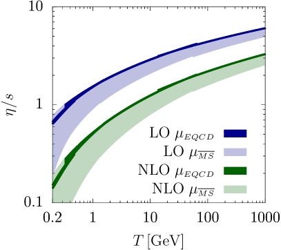
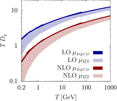
Figure 1: (a) The shear viscosity to entropy density ratio and (b) baryon number diffusion coefficient as a function of temperature, at leading-order (LO) and at next-to-leading order (NLO) for different choices of the running coupling. The solid band fixes the coupling using the two-loop EQCD value with $\mu_{EQCD}=(2.7\leftrightarrow 4\pi)T$, while the shaded band uses the standard $\overline{\mathrm{MS}}$ two-loop coupling with $\mu_{\overline{\mathrm{MS}}}=(\pi\leftrightarrow 4\pi)T$ ; the corresponding values of $\alpha_{s}(T)$ are presented in Fig. 8. The dominant NLO correction arises from NLO modifications of $\hat{q}$ as is illustrated Fig. 6. The uncertainty arising from gain terms which are only estimated (and not computed) is shown in Fig. 9.

Our main results are presented in Section 5, but we will present one “summary” result right away in Figure 1. The figure shows the ratio of the shear viscosity to the entropy density, computed at LO and NLO. The temperature enters in the choice of renormalized coupling and the number of quark species (there are slight discontinuities where we cross quark-number “thresholds”). The solid thinner band represents our “best estimate” based on 2-loop renormalization group flow from the $Z$-pole and the coupling fixed via the EQCD choice of Laine and Schröder Laine:2005ai . The renormalization uncertainty is estimated by varying the scale $\mu_{EQCD}$ over the range $\mu_{EQCD}=(2.7\leftrightarrow 4\pi)T$. The wider bands represent fixing $g^{2}$ from the scale $\pi T$ to $4\pi T$ with the standard ${\overline{\rm MS}}$ approach, to indicate the importance of the renormalization uncertainty. The plot shows that next-to-leading order corrections lower the shear viscosity by a factor of two at high temperatures $T\sim 1000\,{\rm GeV}$, and by a factor of four for physically relevant temperatures, $T\sim 250\,{\rm MeV}$. This large change is suggestive that the true value of $\eta/s$ is smaller than the leading-order perturbative estimate, but it also signals severe convergence problems in the perturbative expansion, even for surprisingly large temperatures or, equivalently, small values of $g$. The figure also shows the analogous result for the (light) quark diffusion coefficient, which displays very similar coupling dependence. We present more results and discussion in later sections, but we point out now that the largest NLO correction arises from NLO modifications of $\hat{q}$ – see Fig. 6. Accurate fits of or NLO results for $\eta/s$ as a function of coupling are provided in an appendix.

Having finished a quick summary of the problem, our approach, and our main conclusions, we now summarize the content of the remainder of the paper. In Section 2 we review the definition of transport coefficients and their calculation within the kinetic theory of Arnold, Moore, and Yaffe Arnold:2002zm . In Section 3 we show how to interpret parts of the leading-order calculation in terms of transverse and longitudinal momentum diffusion and of identity-changing processes. The NLO effects take the form of these three effects, plus a shift in the rate of ${1\leftrightarrow 2}$ splittings, and can therefore be efficiently included once we express the problem in terms of these pieces. We do this in Section 4, with special attention to the “overlap” regions between these processes. With all pieces available, we present the main results in Section 5. We also decompose the NLO correction into the respective pieces to see which are most influential. Some technical details, together with fits for our NLO results as a function of the coupling, are postponed to the appendices.

2 Ingredients

Let us start by briefly summarizing how the transport coefficients we investigate are defined and how they have been computed to leading order in the Effective Kinetic Theory (EKT). Transport coefficients characterize a system’s response to weak, slowly varying inhomogeneities or external forces. In the case of the viscosity, if the flow velocity of the plasma is nonuniform, then the stress-energy tensor (which defines the flux of momentum density) departs from its perfect fluid form. In the local (Landau-Lifshitz) fluid rest frame at a point $x$, the stress tensor, to first order in the velocity gradient, has the form

$$\langle T_{ij}(x)\rangle=\delta_{ij}\,\langle{{\cal P}}\rangle-\eta\sigma_{ij}-\zeta\,\delta_{ij}\,\nabla^{l}\,u_{l}\,,\quad\sigma_{ij}\equiv\nabla_{i}\,u_{j}+\nabla_{j}\,u_{i}-{\textstyle\frac{2}{3}}\,\delta_{ij}\,\nabla^{l}\,u_{l}\,,$$ (1)

where the metric is the “mostly-plus” one, ${{\cal P}}$ is the equilibrium pressure associated with the energy density $\langle T_{00}(x)\rangle=\epsilon$, and the coefficients $\eta$ and $\zeta$ are known as the shear and bulk viscosities, respectively. The flow velocity ${\bm{u}}$ equals the momentum density divided by the enthalpy density $\epsilon+{\cal P}=sT$. We will only be concerned with the shear viscosity in this paper; the bulk viscosity requires a more complicated analysis, which has been carried out at leading order in Jeon:1994if ; Jeon:1995zm for a scalar theory and in Arnold:2006fz for a gauge theory with massless quarks. The charm contribution has been computed in Laine:2014hba . Additional coefficients such as $\tau_{\pi}$ would appear at higher order in the gradient expansion Baier:2007ix ; Bhattacharyya:2008jc ; Romatschke:2009kr ; Haehl:2015pja , but we leave their evaluation for a future investigation.

In the presence of further conserved global charges beyond four-momentum, such as baryon or lepton number, the associated charge density $n\equiv j^{0}$ and current density ${\bm{j}}$ satisfy a diffusion equation,

$$\langle{{\bm{j}}}\rangle=-D\>{\bm{\nabla}}\langle n\rangle\,,$$ (2)

in the local (Landau-Lifshitz) rest frame of the medium. The coefficient $D$ is called the diffusion constant.

When (some of) the diffusing species of excitations carry electric charge, as is the case for baryon and lepton number, the diffusion constants for these charged species determine the electric conductivity $\sigma$ through an Einstein relation (see Refs. Arnold:2000dr ; Arnold:2003zc ). If the net number of each species of charge carriers is conserved, then

$$\sigma=\sum_{a}\,e_{a}^{2}\,D_{a}\,\frac{\partial n_{a}}{\partial\mu_{a}}\,,$$ (3)

where the sum runs over the different species or flavors of excitations with $e_{a}$, $D_{a}$ and $\mu_{a}$ the corresponding electric charge, diffusion constant and chemical potential, respectively.

These transport coefficients all find a field-theoretical definition through Kubo-type formulae relating them to the zero-frequency (transport) limit of the spectral functions of two-point correlators of the appropriate operators (the stress-energy tensor or other conserved currents). However, for a leading- and next-to-leading-order perturbative evaluation, the diagrammatic approach that would result from a direct application of these Kubo formulae would require cumbersome resummations to all orders of many classes of sub-diagrams. It is thus more convenient to use the linearized version Arnold:2003zc of the EKT developed in Arnold:2002zm . Solving the linearized theory automatically accounts for the needed resummations. The leading-order equivalence between the diagrammatic and kinetic approaches has been proven in Jeon:1994if for a scalar theory and in Aarts:2002tn ; Aarts:2004sd ; Aarts:2005vc ; Gagnon:2006hi ; Gagnon:2007qt for gauge theories.

The leading-order EKT introduced in Arnold:2002zm is given by this Boltzmann equation

$$\left[\frac{\partial}{\partial t}+{\bm{v}}_{\bm{p}}\cdot\frac{\partial}{\partial{\bm{x}}}+{\bm{F}}_{\rm ext}^{a}\cdot\frac{\partial}{\partial{\bm{p}}}\right]f^{a}({\bm{p}},{\bm{x}},t)=-C_{a}[f]\stackrel{{\scriptstyle\mathrm{LO}}}{{=}}-\bigg{(}C_{a}^{{2\leftrightarrow 2}}[f]+C_{a}^{{1\leftrightarrow 2}}[f]\bigg{)}\,,$$ (4)

where $f^{a}({\bm{p}},{\bm{x}},t)=dN^{a}/d^{3}{\bm{x}}d^{3}{\bm{p}}$ is the phase space distribution function for the excitation (gluon, quark, antiquark ) of index $a$. The leading-order collision operator encodes the contribution of tree-level ${2\leftrightarrow 2}$ scattering processes, with Hard-Loop resummed propagators in the soft-sensitive channels, as well as collinear, effective ${1\leftrightarrow 2}$ processes resumming the effect of an infinite number of soft scatterings. Both processes contribute to order $g^{4}T$ to the collision operator; a subset of $C_{a}^{{2\leftrightarrow 2}}[f]$ is logarithmically enhanced, $g^{4}T\ln(1/g)$, due to the aforementioned sensitivity to the soft scale $gT$. $C_{a}^{{2\leftrightarrow 2}}[f]$ and $C_{a}^{{1\leftrightarrow 2}}[f]$ are described in detail in Arnold:2002zm ; Arnold:2003zc .

We now proceed to the gradient expansion of Eq. (4), following the notation of Arnold:2000dr . Schematically, $f^{a}=f_{0}^{a}+f_{0}(1{\pm}f_{0})[f_{1}^{a}+f_{2}^{a}+\ldots]$, where $f_{0}^{a}$ is the equilibrium distribution, $f_{0}^{a}=(\exp(-\beta u^{\mu}P_{\mu}-q^{a}_{\alpha}\beta\mu)\mp 1)^{-1}$, which is determined by the Boltzmann equation at zeroth order in the gradients, $C_{a}[f_{0}]=0$. The inverse temperature $\beta$, the chemical potential $\mu$, and the flow velocity $u^{\mu}$ are functions of $(t,{\bm{x}})$ and obey the equations of ideal hydrodynamics. We will consider $u^{i}(t,{\bm{x}})$ and $\mu(t,{\bm{x}})$ to be small perturbations on top of an approximately homogeneous background. The charge of species $a$ under conserved charge $Q_{\alpha}$ is $q_{\alpha}^{a}$, where $\alpha$ is a label for the flavor symmetry of interest (i.e. quark number in our case).

Substituting $f_{0}^{a}$ into the lefthand side of the Boltzmann equation, Eq. (4), yields a source for the first dissipative correction, which (after using the hydrodynamic equations of motion) is proportional to the strains Teaney:2009qa

$$X_{i\cdots j}\equiv\begin{cases}\;\nabla_{i}\,\mu_{\alpha}\,,&\mbox{(diffusion),}\cr\frac{1}{\sqrt{6}}\left(\nabla_{i}u_{j}+\nabla_{j}u_{i}-\frac{2}{3}\,\delta_{ij}\nabla\cdot{\bm{u}}\right)\,,&\mbox{(shear viscosity),}\cr\end{cases}$$ (5)

depending on whether we are considering chemical potential fluctuations (diffusion) or velocity fluctuations (shear viscosity). The source takes the form

$${\cal S}^{a}({\bm{p}})\equiv \beta^{2}{\cal S}^{a}_{{i\cdots j}}({\bm{p}})X_{{i\cdots j}}\,,$$

$$= -\beta q^{a}f_{0}^{a}(p)[1{\pm}f_{0}^{a}(p)]\,I_{i\cdots j}(\hat{\bm{p}})X_{{i\cdots j}}\,.$$ (6)

Here $q^{a}$ denotes the relevant conserved charge carried by species $a$ associated with the transport coefficient of interest,

$$q^{a}\equiv\begin{cases}q^{a}_{\alpha}\,,&\mbox{(diffusion),}\cr|{\bm{p}}|\,,&\mbox{(shear viscosity).}\cr\end{cases}$$ (7)

$I_{i\cdots j}$ is the unique $\ell=1$ or $\ell=2$ rotationally covariant tensor depending only on $\hat{\bm{p}}$,

$$I_{i\cdots j}(\hat{\bm{p}})\equiv\begin{cases}\;\hat{p}_{i}\,,&\ell=1\mbox{ (conductivity/diffusion),}\cr\sqrt{\frac{3}{2}}\,(\hat{p}_{i}\hat{p}_{j}-{\frac{1}{3}}\delta_{ij})\,,&\ell=2\mbox{ (shear viscosity).}\cr\end{cases}$$ (8)

The normalization on $I_{i\cdots j}$ was chosen so that

$$I_{i\cdots j}(\hat{\bm{p}})\,I_{i\cdots j}(\hat{\bm{p}})=1,$$ (9)

and more generally,

$$I_{i\cdots j}(\hat{\bm{p}})\,I_{i\cdots j}(\hat{\bm{k}})=P_{\ell}(\hat{\bm{p}}\cdot\hat{\bm{k}}),$$ (10)

where $P_{\ell}(x)$ is the $\ell$’th Legendre polynomial.

The linearized kinetic equation may be written compactly as

$${\cal S}^{a}({\bm{p}})=({\cal C}f_{1})^{a}({\bm{p}})\,,$$ (11)

where ${\cal C}$ is a linearized collision operator defined below. To linear order the first dissipative correction must be proportional to the driving term $X$, allowing us to define the proportionality coefficient $\chi_{i\cdots j}({\bm{p}})$,

$$f_{1}^{a}({\bm{p}})\equiv\beta^{2}X_{{i\cdots j}}\,\chi_{{i\cdots j}}^{a}({\bm{p}})\equiv\beta^{2}X_{i\cdots j}\,I_{i\cdots j}(\hat{\bm{p}})\>\chi^{a}(p)\,,$$ (12)

where we have also used rotational invariance of the collision operator (in the rest frame) to define a scalar proportionality coefficient $\chi(p)$, which describes how the departure from equilibrium varies as a function of the magnitude of the momentum.

The first-order transport coefficients are then obtained from the kinetic-theory expressions for $T^{\mu\nu}$ and for the conserved current $J^{\mu}_{\alpha}$ associated to the conserved charge $Q_{\alpha}$, i.e.,

$$T^{\mu\nu}({\bm{x}},t)=\int\frac{d^{3}{\bm{p}}}{(2\pi)^{3}}\frac{p^{\mu}p^{\nu}}{p}\sum_{a}\nu_{a}f^{a}({\bm{p}},{\bm{x}},t),\quad J_{\alpha}^{\mu}({\bm{x}},t)=\int\frac{d^{3}{\bm{p}}}{(2\pi)^{3}}\frac{p^{\mu}}{p}\sum_{a}\nu_{a}q^{a}_{\alpha}f^{a}({\bm{p}},{\bm{x}},t),$$ (13)

where $\nu_{a}$ is the spin and color degeneracy of the excitation $a$ ($2N_{c}$ for quarks and antiquarks, $2(N_{c}^{2}-1)$ for gluons). Upon inserting the first-order deviation $f^{1}$ in these equations, the first-order coefficients are easily recovered. Hence, the solution of the first-order, linear Eq. (11) yields $\eta$ and $D$.

As in Arnold:2000dr ; Arnold:2003zc , we will solve Eq. (11) and its NLO extension by means of a variational method. To this end, we introduce the inner product

$$\Big{(}f,g\Big{)}\equiv\beta^{3}\sum_{a}\,\nu_{a}\!\int\frac{d^{3}{\bm{p}}}{(2\pi)^{3}}\>\,f^{a}({\bm{p}})\,g^{a}({\bm{p}})\,.$$ (14)

The linearized collision operator ${\cal C}$ is symmetric with respect to this inner product, and is given by variation of the quadratic form

$$({\cal C}f_{1})^{a}({\bm{p}})=\frac{(2\pi)^{3}}{\beta^{3}\nu_{a}}\frac{\delta\,}{\delta f_{1}^{a}({\bm{p}})}{\textstyle{\frac{1}{2}}}(f_{1},{\cal C}f_{1})\,.$$ (15)

${\cal C}$ is a positive semi-definite operator, and is strictly positive definite in the $\ell{=}1$ and $\ell{=}2$ channels relevant for diffusion or shear viscosity. As we will show, some NLO contributions are negative, so some care will be needed in defining a positive definite $\mathcal{C}_{\mathrm{NLO}}$. Once that is taken care of, the linearized Boltzmann equation (11) at LO and NLO is precisely the condition for maximizing the functional

$$\beta^{4}\mathcal{Q}[\chi]\equiv\Big{(}f_{1},{\cal S}\Big{)}-{\textstyle{\frac{1}{2}}}\,\Big{(}f_{1},{\cal C}\,f_{1}\Big{)}.$$ (16)

Note that the maximized $\mathcal{Q}$ determines the rate per volume at which work is dissipated into heat; $\beta\mathcal{Q}$ then gives the rate per volume of entropy production. This structure is valid at LO and NLO, so we have not explicitly labeled ${\cal C}$ and $f_{1}$ in that respect. The strains $X_{{i\cdots j}}$ may be pulled out of the integrals, and then rotational invariance of the measure and collision operator guarantees that

$$T^{4}\Big{(}f_{1},{\cal C}f_{1}\Big{)}= \>\frac{X^{2}}{2\ell+1}\Big{(}\chi_{{i\cdots j}},{\cal C}\,\chi_{{i\cdots j}}\Big{)},$$ (17)

$$T^{4}\Big{(}f_{1},{\cal S}\Big{)}= \>\frac{X^{2}}{2\ell+1}\Big{(}\chi_{{i\cdots j}},S_{{i\cdots j}}\Big{)},$$ (18)

where $X^{2}=X_{i\cdots j}\,X_{i\cdots j}$.

The explicit forms of the source and LO collision parts of this quadratic functional are

$$T^{4}\Big{(}f_{1},{\cal S}\Big{)} {}=\frac{X^{2}}{2\ell+1}\sum_{a}\beta^{2}\nu_{a}\int\frac{d^{3}{\bm{p}}}{(2\pi)^{3}}\>f_{0}(p)\,[1\pm f_{0}(p)]\>q^{a}\,\chi^{a}(p)\,,$$ (19)

and

$$\Big{(}f_{1},{\cal C}_{\mathrm{LO}}\,f_{1}\Big{)} {}=\Big{(}f_{1},\mathcal{C}^{{2\leftrightarrow 2}}\,f_{1}\Big{)}+\Big{(}f_{1},\mathcal{C}^{{1\leftrightarrow 2}}\,f_{1}\Big{)}\,.$$ (20)

The ${2\leftrightarrow 2}$ contribution reads, after symmetrization of the departures from equilibrium Arnold:2003zc

$$\Big{(}f_{1},{\cal C}^{2\leftrightarrow 2}\,f_{1}\Big{)}\equiv \,\frac{\beta^{3}}{8}\sum_{abcd}\int_{{\bm{p}}{\bm{k}}{\bm{p}}^{\prime}{\bm{k}}^{\prime}}\frac{\bigl{|}{\mathcal{M}}^{ab}_{cd}({\bm{p}},{\bm{k}};{\bm{p}}^{\prime},{\bm{k}}^{\prime})\bigr{|}^{2}}{(2p)(2k)(2p^{\prime})(2k^{\prime})}\,(2\pi)^{4}\,\delta^{(4)}(P{+}K{-}P^{\prime}{-}K^{\prime})$$

$${}\times f^{a}_{0}(p)\,f^{b}_{0}(k)\,[1{\pm}f^{c}_{0}(p^{\prime})]\,[1{\pm}f^{d}_{0}(k^{\prime})]\,\Bigl{[}f_{1}^{a}({\bm{p}})+f_{1}^{b}({\bm{k}})-f_{1}^{c}({\bm{p}}^{\prime})-f_{1}^{d}({\bm{k}}^{\prime})\Bigr{]}^{2}\,,$$ (21)

where $\int_{\bm{p}}$ is shorthand for $\int d^{3}{\bm{p}}/(2\pi)^{3}$ and $\bigl{|}{\mathcal{M}}^{ab}_{cd}({\bm{p}},{\bm{k}};{\bm{p}}^{\prime},{\bm{k}}^{\prime})\bigr{|}^{2}$ is the matrix element squared for the $ab\leftrightarrow cd$ process, summed over all spins polarizations and colors and Hard Thermal Loop (HTL) resummed Braaten:1989mz ; Frenkel:1989br in the IR-sensitive cases. A complete list of these matrix elements appears in Arnold:2002zm ; Arnold:2003zc . The ${1\leftrightarrow 2}$ contribution reads instead Arnold:2003zc

$$\Big{(}f_{1},{\cal C}^{1\leftrightarrow 2}\,f_{1}\Big{)}\equiv \,\frac{\beta^{3}}{2}\sum_{abc}\int d\Omega_{\hat{\bm{n}}}\int_{0}^{\infty}dp\int_{0}^{p}dk\;\gamma^{a}_{bc}(p;p-k,k)\;$$

$$\times f_{0}^{a}(p)\,[1{\pm}f_{0}^{b}(p-k)]\,[1{\pm}f_{0}^{c}(k)]\>\Bigl{[}f_{1}^{a}(p\hat{\bm{n}})-f_{1}^{b}((p-k)\hat{\bm{n}})-f_{1}^{c}(k\hat{\bm{n}})\Bigr{]}^{2}\,.$$ (22)

The splitting rate is given by

$$\gamma^{a}_{bc}(p;p-k,k)=\frac{g^{2}d_{R_{b}}C_{R_{b}}}{64\pi^{4}}\left\{\begin{array}[]{cc}\frac{p^{4}+k^{4}+(p-k)^{4}}{p^{3}k^{3}(p-k)^{3}}&g\leftrightarrow gg\\ \frac{p^{2}+(p-k)^{2}}{p^{2}(p-k)^{2}k^{3}}&q\leftrightarrow qg\\ \frac{(p-k)^{2}+k^{2}}{(p-k)^{2}k^{2}p^{3}}&g\leftrightarrow q\bar{q}\end{array}\right.\int\frac{d^{2}h}{(2\pi)^{2}}\;2\mathbf{h}\cdot{\rm Re}\,\mathbf{F}_{b}(\mathbf{h})\,,$$ (23)

where $\mathbf{h}={\bm{p}}\times{\bm{k}}$ is a transverse, two-dimensional vector related to the transverse momentum picked up during the splitting process. $d_{R_{b}}$ and $C_{R_{b}}$ are the dimension and quadratic Casimir operator of the representation $R$ of the particle $b$. A complete leading-order treatment of collinear radiation must consistently resum the effect of the many soft, transverse collisions to account for the Landau-Pomeranchuk-Migdal (LPM) effect Baier:1994bd ; Baier:1996kr ; Zakharov:1996fv ; Zakharov:1997uu ; Arnold:2002ja . This is achieved through the following integral equation for $\mathbf{F}_{b}(\mathbf{h})$:

$$2\mathbf{h} = i\delta E(\mathbf{h})\mathbf{F}_{b}(\mathbf{h})+\int\frac{d^{2}q_{\perp}}{(2\pi)^{2}}\bar{C}(q_{\perp})\bigg{\{}\left(C_{R_{b}}-\frac{C_{A}}{2}\right)[\mathbf{F}_{b}(\mathbf{h})-\mathbf{F}_{b}(\mathbf{h}-k\mathbf{q}_{\perp})]$$ (24)

$$+\frac{C_{A}}{2}[\mathbf{F}_{b}(\mathbf{h})-\mathbf{F}_{b}(\mathbf{h}+p\mathbf{q}_{\perp})]+\frac{C_{A}}{2}[\mathbf{F}_{b}(\mathbf{h})-\mathbf{F}_{b}(\mathbf{h}-(p-k)\mathbf{q}_{\perp})]\bigg{\}}.$$

For the case of $g\to q\bar{q}$, $C_{R_{b}}-C_{A}/2=C_{F}-C_{A}/2$ multiplies the term with $\mathbf{F}_{b}(\mathbf{h}-p\mathbf{q}_{\perp})$ rather than $\mathbf{F}_{b}(\mathbf{h}-k\mathbf{q}_{\perp})$. The equation depends on two inputs, $\bar{C}(q_{\perp})$ and $\delta E(\mathbf{h},p,k)$. The former is the leading-order transverse scattering kernel $C(q_{\perp})$ in units of the Casimir factor, Arnold:2001ba ; Aurenche:2002pd

$$\bar{C}(q_{\perp})\equiv\frac{C_{R}(q_{\perp})}{C_{R}}=\frac{g^{2}Tm_{\scriptscriptstyle D}^{2}}{q_{\perp}^{2}(q_{\perp}^{2}+m_{\scriptscriptstyle D}^{2})}.$$ (25)

$\delta E$ is the energy difference between the initial and final collinear particles. It reads

$$\delta E(\mathbf{h})=\frac{h^{2}}{2pk(p-k)}+\frac{m^{2}_{\infty\,c}}{2k}+\frac{m^{2}_{\infty\,b}}{2(p-k)}-\frac{m^{2}_{\infty\,a}}{2p},$$ (26)

where $m_{\infty\,a}^{2}$ is the asymptotic mass of the particle $a$. For gluons $m_{\infty\,g}^{2}\equiv M_{\infty}^{2}=m_{\scriptscriptstyle D}^{2}/2$ (with $m_{\scriptscriptstyle D}^{2}=g^{2}T^{2}/3(T_{A}+T_{F}N_{f})$), for quarks $m_{\infty\,q}^{2}\equiv m_{\infty}^{2}=C_{F}g^{2}T^{2}/4$.

The maximization of the functional (16) is then carried out using a variational Ansatz of form

$$\chi(p)=\sum_{m=1}^{K}c_{m}\phi^{(m)}(p)\,,\qquad\phi^{(m)}(p)=\frac{p^{\ell-1}(p/T)^{m-1}}{(1+p/T)^{K-3/2}}\,,$$ (27)

which, when substituted into Eq. (16), transforms its extremization into a matrix algebra problem Arnold:2000dr . Our choice of functional basis is motivated by the need Arnold:2003zc to allow infrared behavior of form $\propto p^{\ell-1}$ and ultraviolet behavior of form $\propto p^{\ell-1/2}$. The variational procedure is only guaranteed to converge to the right answer as the functional basis becomes complete, but in practice we see good convergence above 4 functions. Later, in our numerical results, we will use 6 basis functions, but our results shift by less than $10^{-4}$ when we make the basis still larger.

3 Reorganization of the LO quadratic functional

The effective kinetic theory introduced in Arnold:2002zm has been extended to next-to-leading order in Ghiglieri:2015ala for the case where one follows the evolution of a dilute set of high-energy particles of typical energy $E$ interacting with an equilibrated medium at a temperature $T$ such that $\exp(-E/T)\ll 1$, which is a sensible approximation for the evolution of the leading partons in a jet. There, we found that a reorganization of the form of the LO collision operator was necessary to systematically compute NLO corrections. Specifically, $\mathcal{O}(g)$ NLO corrections can only occur where one or more lines carry a soft $\mathcal{O}(gT)$ momentum, because only there do statistical functions give rise to a $1/g$ enhancement of loop level effects. But transport coefficients are only sensitive to hard $\mathcal{O}(T)$ momenta. So NLO corrections only occur when there is a momentum hierarchy within a diagram. In such cases one can always re-express the diagram as an effective process. When the soft particle is a gluon and does not change particle identity, the process can be understood as giving rise to momentum diffusion; when the exchanged particle is a quark and therefore changes quantum numbers, it is a conversion process. One can already isolate such processes at the leading order. Doing so will make it easier to see how to incorporate NLO processes.

In the diffusion case, the action of the soft gluon exchange is to randomize (diffuse) the momentum of the hard particles by small, $\mathcal{O}(g)$ amounts that can be described by a Fokker-Planck equation. The drag, longitudinal and transverse momentum diffusion coefficients appearing in the Fokker-Planck equation can be defined field-theoretically in terms of Wilson-line operators supported on light fronts, which can in turn be evaluated in analytical form using the light-cone techniques mentioned in the introduction. In the conversion case, the soft quark exchange converts a hard quark (gluon) into a gluon (quark) of the same momentum, up to $\mathcal{O}(gT)$. Again, a light-front Wilson line definition for the conversion rate was introduced in Ghiglieri:2015ala , leading to a simple closed form expression. At NLO, the diffusion and conversion rates receive $\mathcal{O}(g)$ corrections, which were computed in CaronHuot:2008ni ; Ghiglieri:2013gia ; Ghiglieri:2015ala . These, together with corrections to the collinear ${1\leftrightarrow 2}$ rate and a new, semi-collinear process (which only contributes starting from NLO), constitute the entirety of the NLO corrections to the EKT in the “dilute-hard” approximation appropriate for energy loss.

For computing the transport coefficients we will first show (again) how the effect of soft-gluon exchange can be reorganized into a Fokker-Planck equation in Section 3.1. However, in order to conserve energy and momentum, the Fokker-Planck equation must be supplemented by gain terms, which describe precisely how the momentum lost by a parton in the bath is redistributed. This redistribution of energy and momentum is unimportant for determining the energy loss, but plays an essential role in determining the transport coefficients. The computation of these gain terms is not amenable to an evaluation using light-cone techniques since more than one light-like particle is involved, and therefore computing the gain terms constitutes a major obstacle to computing transport coefficients at NLO. We will use the LO analysis in this section to motivate a NLO Ansatz for the gain terms in Section 4. The treatment of soft fermion exchange and conversions is analogous and will be discussed in Section 3.2.

3.1 Soft gluon exchange

We will now analyze soft gluon exchange shown in Fig. 2.

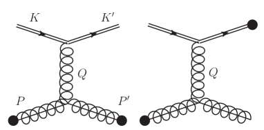
Figure 2: Diagrammatic representation of the diffusion and gain terms in soft gluon exchange processes. Double lines are hard quarks or gluons and the intermediate gluon is soft. The blobs represent the insertion of the deviation from equilibrium $f_{1}({\bm{p}})$. The diagram on the left is a diffusion term, entering in $(f_{1}^{g}({\bm{p}})-f_{1}^{g}({\bm{p}}^{\prime}))^{2}$, whereas the one on the right is a gain term recording the correlations between momentum ${\bm{p}}$ and ${\bm{k}}$.

Intuitively, the effect of soft gluon exchange on the evolution of the system can be summarized by a Fokker-Planck equation. Anticipating the results of this section, the Fokker-Planck collision kernel can be written

$$({\cal C}_{\mathrm{diff}}^{{2\leftrightarrow 2}}f_{1})^{a}({\bm{p}})=-\frac{1}{2}\frac{\partial}{\partial p^{i}}\,\hat{q}^{ij}_{a}\,f_{0}^{a}(p)(1{\pm}f_{0}^{a}(p))\frac{\partial f_{1}^{a}({\bm{p}})}{\partial p^{j}}+\mbox{gain-terms}\,,$$ (28)

where

$$\hat{q}^{ij}_{a}=\hat{q}_{a,L}\hat{p}^{i}\hat{p}^{j}+\tfrac{1}{2}\hat{q}_{a}\left(\delta^{ij}-\hat{p}^{i}\hat{p}^{j}\right)$$ (29)

records the momentum diffusion parallel and perpendicular to the particle’s momentum through $\hat{q}_{L}$ and $\hat{q}$ respectively. The gain terms are necessary to conserve energy an momentum, and record how the energy lost by a parton with momentum ${\bm{k}}$ is redistributed to particles with momentum ${\bm{p}}$. The gain terms will take the following form:

$$\mbox{gain-terms}=\frac{1}{2}\frac{\partial}{\partial p^{i}}\left(f_{0}^{a}(p)(1{\pm}f_{0}^{a}(p))\,\sum_{b}\nu_{b}\!\int_{\bm{k}}{\mathcal{C}}^{ij}_{ab}(\hat{\bm{p}}\cdot\hat{\bm{k}})\,f_{0}^{b}(k)(1\pm f_{0}^{b}(k))\frac{\partial f_{1}^{b}({\bm{k}})}{\partial k^{j}}\right)\,.$$ (30)

Here the angular function ${\mathcal{C}}^{ij}_{ab}(\hat{\bm{p}}\cdot\hat{\bm{k}})$ determines $\hat{q}^{ij}_{a}$

$$\hat{q}^{ij}_{a}=\sum_{b}\nu_{b}\int_{\bm{k}}f_{0}^{b}(k)(1\pm f_{0}^{b}(k))\,{\mathcal{C}}_{ab}^{ij}(\hat{\bm{p}}\cdot\hat{\bm{k}})\,,$$ (31)

and its explicit form given in Eq. (38). It is easily verified that energy and momentum are conserved under the time evolution $(\partial_{t}+v_{\bm{p}}\partial_{\bm{x}})f({\bm{p}})=-({\cal C}f_{1,{\rm diff}})({\bm{p}})$. A simulation and discussion of a similar Fokker-Planck equation (with the gain terms) is given in Hong:2010at .

Now we will derive these equations by analyzing the ${2\leftrightarrow 2}$ collision integral with soft gluon exchange recorded in Eq. (21) and illustrated Fig. 2. The relevant processes are $gg\leftrightarrow gg$, $q_{1}q_{2}\leftrightarrow q_{1}q_{2}$ (and similar ones where $q_{1}$ and/or $q_{2}$ are replaced by their antiquarks), $q_{1}q_{1}\leftrightarrow q_{1}q_{1}$ and $\bar{q}_{1}\bar{q}_{1}\leftrightarrow\bar{q}_{1}\bar{q}_{1}$, $q_{1}\bar{q}_{1}\leftrightarrow q_{1}\bar{q}_{1}$ and finally $q_{1}g\leftrightarrow q_{1}g$ and $\bar{q}_{1}g\leftrightarrow\bar{q}_{1}g$. The LO contribution from soft gluon exchange is obtained by expanding Eq. (21) for $\omega,q\sim gT$, $p,k\sim T$, where $Q=(\omega,{\bm{q}})=P^{\prime}-P$ is the momentum exchange shown in Fig. 2. In more detail, the phase space integration in Eq. (21) is approximated by (see Appendix B.1)

$$\int_{PS}\equiv\int_{{\bm{p}}{\bm{k}}{\bm{p}}^{\prime}{\bm{k}}^{\prime}}(2\pi)^{4}\delta(P+K-P^{\prime}-K^{\prime})\simeq\int_{{\bm{p}}{\bm{k}}}\int\frac{d^{4}Q}{(2\pi)^{4}}\,2\pi\delta(v_{\bm{p}}\cdot Q)\,2\pi\delta(v_{\bm{k}}\cdot Q)\,,$$ (32)

where $v_{\bm{p}}^{\mu}=(1,\hat{\bm{p}})$ and $v_{\bm{k}}^{\mu}=(1,\hat{\bm{k}})$ are light-like vectors in the direction of $\hat{\bm{p}}$ and $\hat{\bm{k}}$. The $t$-channel matrix element in the soft approximation reads Arnold:2002zm ; Arnold:2003zc

$$\frac{|\mathcal{M}^{ab}_{ab}|^{2}_{\mathrm{soft\,g}\,t}}{(2p)^{2}(2k)^{2}} = \frac{\nu_{a}C_{R_{a}}\nu_{b}C_{R_{b}}g^{4}}{d_{A}}\left|G_{\mu\nu}^{R}(Q)v_{\bm{p}}^{\mu}v_{\bm{k}}^{\nu}\right|^{2}\,.$$ (33)

$G_{\mu\nu}^{R}(Q)$ is the retarded, HTL-resummed propagator Braaten:1989mz ; Frenkel:1989br in Coulomb gauge (see App. A). For process with identical particles in the initial or final state, the $u$-channel exchange is equivalent in the soft limit. Finally, in a soft (or diffusive) expansion we may approximate the departures from equilibrium appearing in Eq. (21)

$$\left[f_{1}^{a}({\bm{p}})+f_{1}^{b}({\bm{k}})-f_{1}^{a}({\bm{p}}^{\prime})-f_{1}^{b}({\bm{k}}^{\prime})\right]^{2}=\left[q^{i}\frac{\partial f_{1}^{a}({\bm{p}})}{\partial p^{i}}-q^{j}\frac{\partial f_{1}^{b}({\bm{k}})}{\partial k^{j}}\right]^{2}.$$ (34)

With these approximations the ${2\leftrightarrow 2}$ collision operator in a diffusive approximation takes the form

$$(f_{1},{\cal C}^{2\rightarrow 2}_{\mathrm{diff}}f_{1})\equiv\left.(f_{1},{\cal C}^{2\rightarrow 2}_{\mathrm{diff}}f_{1})\right|_{\rm loss}+\left.(f_{1},{\cal C}^{2\rightarrow 2}_{\mathrm{diff}}f_{1})\right|_{\rm gain}\,,$$ (35)

where

$$\left.(f_{1},{\cal C}^{2\rightarrow 2}_{\scriptscriptstyle\rm diff}f_{1})\right|_{\rm loss}=\frac{1}{2}\beta^{3}\sum_{a}\nu_{a}\,\int_{\bm{p}}f_{0}^{a}(p)(1\pm f_{0}^{a}(p))\,\hat{q}^{ij}_{a}\,\frac{\partial f_{1}^{a}({\bm{p}})}{\partial p^{i}}\frac{\partial f_{1}^{a}({\bm{p}})}{\partial p^{j}}\,,$$ (36)

and the gain terms take the form

$$\left.(f_{1},\mathcal{C}^{{2\leftrightarrow 2}}_{\mathrm{diff}}f_{1})\right|_{\rm gain}\!\!=-\frac{\beta^{3}}{2}\sum_{ab}\nu_{a}\nu_{b}\!\int_{{\bm{p}}{\bm{k}}}\!\!f_{0}^{a}(p)(1\pm f_{0}^{a}(p))f^{b}_{0}(k)(1\pm f_{0}^{b}(k))\,{\mathcal{C}}_{ab}^{ij}(\hat{\bm{p}}\cdot\hat{\bm{k}})\frac{\partial f_{1}^{a}({\bm{p}})}{\partial p^{i}}\frac{\partial f_{1}^{b}({\bm{k}})}{\partial k^{j}},$$ (37)

where the angular function is

$${\mathcal{C}}_{ab}^{ij}(\hat{\bm{p}}\cdot\hat{\bm{k}})=\frac{g^{4}C_{R_{a}}C_{R_{b}}}{d_{A}}\int\frac{d^{4}Q}{(2\pi)^{4}}|G_{\mu\nu}^{R}(Q)v_{{\bm{p}}}^{\mu}v_{\bm{k}}^{\nu}|^{2}\,2\pi\delta(v_{\bm{p}}\cdot Q)2\pi\delta(v_{\bm{k}}\cdot Q)q^{i}q^{j}\,,$$ (38)

and $\hat{q}^{ij}_{a}$ is given by Eq. (31). Varying the quadratic functional $(f_{1},{\cal C}_{\mathrm{diff}}f_{1})$ according to Eq. (15) we see the Fokker-Planck evolution equations, Eqs. (28) and (30), emerge.

At a technical level, the loss terms arise when the deviations from equilibrium are on the same side of the gluon exchange diagram, and their contribution to the quadratic functional therefore involves $(f_{1}({\bm{p}})-f_{1}({\bm{p}}^{\prime}))^{2}\sim q^{2}(f_{1}^{\prime}({\bm{p}}))^{2}$. This is illustrated by the black dots in Fig. 2 (left). The gain terms describe the correlation between the momenta across the exchange diagram (illustrated by the dots in Fig. 2 (right)), and the quadratic functional involves $(f_{1}({\bm{p}})-f_{1}({\bm{p}}^{\prime}))(f_{1}({\bm{k}}^{\prime})-f_{1}({\bm{k}}))\sim q^{2}f_{1}^{\prime}({\bm{p}})f_{1}^{\prime}({\bm{k}})$. From the point of view of the Fokker-Planck equations this term gives rise to a gain term. But from the point of view of the original Boltzmann equation, this is a cross-correlation between the departures from equilibrium of the two particles. Therefore we will refer to these contributions both a gain terms and as cross terms, depending on the context.

Examining the expression for $\left.(f_{1},{\cal C}_{\mathrm{diff}}^{{2\leftrightarrow 2}}f_{1})\right|_{\rm loss}$, we see that it involves one light-like vector, $v_{\bm{p}}$. Indeed, the expression for $\hat{q}^{ij}$ can be rewritten as the Wightman correlator of soft thermal gauge fields along this light-like direction. Using the causality and KMS properties of such light-like correlators CaronHuot:2008ni , these soft contributions to $\hat{q}$ and $\hat{q}_{\scriptscriptstyle L}$ can be evaluated in closed form Aurenche:2002pd ; Ghiglieri:2015zma ; Ghiglieri:2015ala ,

$$\hat{q}^{a}\bigg{|}_{\mathrm{soft}}=\frac{g^{2}C_{R_{a}}Tm_{\scriptscriptstyle D}^{2}}{2\pi}\ln\frac{\mu_{\perp}}{m_{\scriptscriptstyle D}},\qquad\hat{q}_{\scriptscriptstyle L}^{a}\bigg{|}_{\mathrm{soft}}=\frac{g^{2}C_{R_{a}}Tm_{\scriptscriptstyle D}^{2}}{4\pi}\ln\frac{\sqrt{2}\mu_{\perp}}{m_{\scriptscriptstyle D}}.$$ (39)

Here $gT\ll\mu_{\perp}\ll T$ is a cutoff on the $q_{\perp}\equiv\sqrt{q^{2}-\omega^{2}}$ integration separating the soft from the hard scale. The dependence on this cutoff cancels against the region where $\omega,q{\ \lower-1.2pt\vbox{\hbox{\hbox to0.0pt{$>$\hss}\lower 6.0pt\vbox{\hbox{$\sim$}}}}\ }T$, where the bare matrix elements can be used to evaluate the hard contribution to ${\cal C}^{{2\leftrightarrow 2}}$. The simple form of $\hat{q}$ and $\hat{q}_{\scriptscriptstyle L}$ is a consequence of the fact that light-like separated points are effectively causally disconnected as far as the soft gauge fields are concerned. Using the explicit form of the angular dependence of $f_{1}^{a}({\bm{p}})=\beta^{2}\chi_{{i\cdots j}}({\bm{p}})X_{{i\cdots j}}$ and Eq. (17), straightforward analysis shows that the loss term reduces to

$$\left.\Big{(}\chi_{i\cdots j},{\cal C}^{2\leftrightarrow 2}_{\mathrm{diff}}\,\chi_{i\cdots j}\Big{)}\right|_{\rm loss}=\frac{\beta^{3}}{2}\sum_{a}\nu_{a}\int_{\bm{p}}f^{a}_{0}(p)(1\pm f_{0}^{a}(p))\times\\ \left[(\chi^{a}(p)^{\prime})^{2}\hat{q}^{a}_{\scriptscriptstyle L}\bigg{|}_{\mathrm{soft}}+\frac{\ell(\ell+1)\chi^{a}(p)^{2}}{2p^{2}}\hat{q}^{a}\bigg{|}_{\mathrm{soft}}\right]\,,$$ (40)

which is the most useful form for evaluating the transport coefficients numerically.

The gain terms (Eq. (37)) intrinsically involve two light-like momenta $v_{\bm{p}}$ and $v_{\bm{k}}$ associated with $f_{1}({\bm{p}})$ and $f_{1}({\bm{k}})$. The points on these two light-like rays are causally connected by soft gauge fields, thus the analyticity techniques used for $\hat{q}$ cannot be expected to work. All attempts to extend these techniques to two light-like rays have met with frustration, and ${\mathcal{C}}_{ab}^{ij}(\hat{\bm{p}}\cdot\hat{\bm{k}})$ and its moments must be computed numerically. To this end, using Eq. (17) and the angular dependence of $f_{1}({\bm{p}})=\beta^{2}\chi(p)\,I_{{i\cdots j}}(\hat{\bm{p}})\,X_{{i\cdots j}}$, we may rewrite the gain terms as

$$\left.\Big{(}\chi_{i\cdots j},{\cal C}^{2\leftrightarrow 2}_{\mathrm{diff}}\chi_{i\cdots j}\Big{)}\right|_{\rm gain}=-\,\sum_{ab}\frac{g^{4}\nu_{a}C_{R_{a}}\nu_{b}C_{R_{b}}}{8\pi^{2}d_{A}T^{3}}\int_{{\bm{p}}}\int_{0}^{\infty}dk\,k^{2}\,f_{0}^{a}(p)(1\pm f_{0}^{a}(p))f_{0}^{b}(k)(1\pm f_{0}^{b}(k))\\ \times\left[c_{1}\chi^{a}(p)^{\prime}\chi^{b}(k)^{\prime}+c_{2}\left(\chi^{a}(p)^{\prime}\frac{\chi^{b}(k)}{k}+\chi^{b}(k)^{\prime}\frac{\chi^{a}(p)}{p}\right)+c_{3}\frac{\chi^{a}(p)}{p}\frac{\chi^{b}(k)}{k}\right],$$ (41)

where

$$c_{1}\equiv \int\frac{d\Omega_{{\bm{k}}}}{4\pi}\int\frac{d^{4}Q}{(2\pi)^{4}}\,|G_{\mu\nu}^{R}(Q)v_{\bm{p}}^{\mu}v_{{\bm{k}}}^{\nu}|^{2}\,2\pi\delta(v_{\bm{p}}\cdot Q)\,2\pi\delta(v_{{\bm{k}}}\cdot Q)\,\omega^{2}P_{\ell}(\hat{\bm{p}}\cdot\hat{\bm{k}})\,,$$ (42a)

$$c_{2}\equiv \int\frac{d\Omega_{\bm{k}}}{4\pi}\int\frac{d^{4}Q}{(2\pi)^{4}}\,|G_{\mu\nu}^{R}(Q)v_{\bm{p}}^{\mu}v_{\bm{k}}^{\nu}|^{2}\,2\pi\delta(v_{\bm{p}}\cdot Q)\,2\pi\delta(v_{\bm{k}}\cdot Q)\,\omega^{2}(1-\hat{\bm{p}}\cdot\hat{\bm{k}})P^{\prime}_{\ell}(\hat{\bm{p}}\cdot\hat{\bm{k}})\,,$$ (42b)

$$c_{3}\equiv \int\frac{d\Omega_{\bm{k}}}{4\pi}\int\frac{d^{4}Q}{(2\pi)^{4}}\,|G_{\mu\nu}^{R}(Q)v_{\bm{p}}^{\mu}v_{\bm{k}}^{\nu}|^{2}\,2\pi\delta(v_{\bm{p}}\cdot Q)\,2\pi\delta(v_{\bm{k}}\cdot Q)$$

$$\hskip 79.6678pt\times\left[q_{\perp}^{2}P^{\prime}_{\ell}(\hat{\bm{p}}\cdot\hat{\bm{k}})+\omega^{2}(1-\hat{\bm{p}}\cdot\hat{\bm{k}})\big{(}(1-\hat{\bm{p}}\cdot\hat{\bm{k}})P^{\prime}_{\ell}(\hat{\bm{p}}\cdot\hat{\bm{k}})\big{)}^{\prime}\right]$$ (42c)

are coefficients which must be evaluated numerically. The complicated weights involving $P_{\ell}(\hat{\bm{p}}\cdot\hat{\bm{k}})$ multiplying the matrix elements reflect the angular structure of the collision kernel.

When computing the diffusion coefficient ($\ell=1$), the gluon-mediated gain terms described by Eq. (41) actually vanish. This is because the gluons carry no charge and quarks and antiquarks have opposite charges, so that $\chi^{g}(p)=0$, $\chi^{q}(p)=-\chi^{\bar{q}}(p)$. Thus, the only processes that can give rise to gluon-mediated gain terms are $qq\leftrightarrow qq$, $\bar{q}\bar{q}\leftrightarrow\bar{q}\bar{q}$ and $q\bar{q}\leftrightarrow q\bar{q}$. However, due to their opposite signs, the quark and antiquark contributions end up canceling in the sum of these processes in Eq. (41) (see Hong:2010at for further discussion).

When computing the shear viscosity ($\ell=2$), these integrals are convergent, and $(c_{1},c_{2},c_{3})$ may be evaluated directly (see Appendix B.2 for further details). The UV finiteness of the gain terms was discussed previously in Arnold:2000dr ; Hong:2010at where it was noted that in a leading-log approximation (where the HTL propagator in Eq. (42) is replaced with the bare propagator) the coefficients $c_{1},c_{2},c_{3}$ vanish for $\ell\geq 2$.

As discussed in Section 4, we expect that the functional form of the gain terms in Eq. (41) will remain valid at NLO but the coefficients $c_{1},c_{2}$ and $c_{3}$ will be modified by order $g$ corrections. We will only be able to estimate these modifications and their associated (numerically small) contributions to the NLO shear viscosity.

3.2 Soft quark exchange

We will now analyze soft fermion exchange shown in Fig. 3, which parallels the soft gluon exchange described in the previous section. In this case, a hard quark with momentum ${\bm{p}}$ is converted into a hard gluon with approximately the same momentum through the soft fermion exchange. (The reverse process is also possible, and the set of matrix elements involved in this process are $q\bar{q}\leftrightarrow gg$, $qg\leftrightarrow qg$, and $\bar{q}g\leftrightarrow\bar{q}g$.)

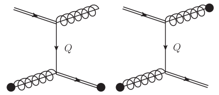
Figure 3: Diagrammatic representation of the conversion and gain terms in soft quark exchange processes. The graphical notation is the same as in Fig. 2 and the intermediate quark is soft (single line). The diagram on the left is a conversion term, entering in $(f_{1}^{q}({\bm{p}})-f_{1}^{g}({\bm{p}}))^{2}$, whereas the one on the right is a gain term.

The dynamics of the conversion process are summarized by a set of rate equations Hong:2010at ; Ghiglieri:2015ala

$$\left(\partial_{t}+v_{\bm{p}}\cdot\partial_{\bm{x}}\right)f^{q}({\bm{p}})= -\Gamma^{\rm conv}_{q\rightarrow g}(p)\;f_{0}^{q}(p)(1+f_{0}^{g}(p))\;\left[f_{1}^{q}({\bm{p}})-f_{1}^{g}({\bm{p}})\right]+\mbox{gain-term}\,,$$ (43a)

$$\left(\partial_{t}+v_{\bm{p}}\cdot\partial_{\bm{x}}\right)f^{\bar{q}}({\bm{p}})= -\Gamma^{\rm conv}_{q\rightarrow g}(p)\;f_{0}^{q}(p)(1+f_{0}^{g}(p))\;\left[f_{1}^{\bar{q}}({\bm{p}})-f_{1}^{g}({\bm{p}})\right]-\mbox{gain-term}\,,$$ (43b)

$$\left(\partial_{t}+v_{\bm{p}}\cdot\partial_{\bm{x}}\right)f^{g}({\bm{p}})= -\sum_{q}\Gamma^{\rm conv}_{g\rightarrow q}(p)\;f_{0}^{g}(p)(1-f_{0}^{q}(p))\;\left[f_{1}^{g}({\bm{p}})-f_{1}^{q}({\bm{p}})\right]$$ (43c)

$$\qquad-\sum_{\bar{q}}\Gamma^{\rm conv}_{g\rightarrow\bar{q}}(p)\;f_{0}^{g}(p)(1-f_{0}^{q}(p))\;\left[f_{1}^{g}({\bm{p}})-f_{1}^{\bar{q}}({\bm{p}})\right]\,.$$

The conversion rates $\Gamma_{q\rightarrow g}^{\rm conv}(p)$ at leading and next-to-leading order are given by Eq. (56) and Eq. (65) respectively Ghiglieri:2015ala , and the gluon conversion rate is

$$\Gamma^{\rm conv}_{g\rightarrow q}=\frac{\nu_{q}}{\nu_{g}}\Gamma_{q\rightarrow g}^{\rm conv}\,.$$ (44)

The gain term is necessary to conserve baryon number under time evolution. Indeed, the gain term records how the baryon charge associated with conversion of a quark of momentum ${\bm{k}}$ to a gluon is balanced by an increase of quarks (or decrease of anti-quarks) of momentum ${\bm{p}}$. We will show that the gain term takes the form

$$\mbox{gain-term}=\frac{f_{0}^{q}(p)(1+f_{0}^{g}(p))}{2p}\int_{\bm{k}}\frac{f_{0}^{q}(k)(1+f_{0}^{g}(k))}{k}\,{\mathcal{C}}_{q\rightarrow g}^{\rm conv}(\hat{\bm{p}}\cdot\hat{\bm{k}})\left(f_{1}^{q}({\bm{k}})-f_{1}^{\bar{q}}({\bm{k}})\right)\,,$$ (45)

where ${\cal C}_{q\rightarrow g}^{\rm conv}(\hat{\bm{p}}\cdot\hat{\bm{k}})$ (which is given explicitly below in Eq. (55)) is a squared matrix element which specifies the angular structure of the conversion process. The angular average of ${\cal C}_{q\rightarrow g}^{\rm conv}(\hat{\bm{p}}\cdot\hat{\bm{k}})$ determines the conversion coefficient $\Gamma_{q\rightarrow g}^{\rm conv}$,

$$p\,\Gamma_{q\rightarrow g}^{\rm conv}(p)=\int_{\bm{k}}\frac{f_{0}^{q}(k)(1+f_{0}^{g}(k))}{k}\mathcal{C}_{q\rightarrow g}^{\rm conv}(\hat{\bm{p}}\cdot\hat{\bm{k}})\,.$$ (46)

It is straightforward to show that with the gain and loss terms the total baryon number is conserved under the evolution specified by Eq. (43).

To derive these results we return to the ${2\leftrightarrow 2}$ collision integrals with soft fermion exchange. The phase space integral and soft approximations are given in the previous section, Eq. (32). The relevant processes are Compton scattering and pair annihilation, $qg\leftrightarrow gq$, $\bar{q}g\leftrightarrow qg$, and $gg\leftrightarrow q\bar{q}$. The HTL-resummed matrix elements are Arnold:2002zm ; Arnold:2003zc

$$\frac{\left|{\mathcal{M}}^{q\bar{q}}_{gg}\right|^{2}_{\mathrm{soft\,q}\,t}}{(2p)(2k)(2p^{\prime})(2k^{\prime})} = \frac{4d_{F}C_{F}^{2}g^{4}}{16pp^{\prime}kk^{\prime}}\mathrm{Tr}[i\not{P}S_{R}(Q)i\not{K}S_{A}(Q)]\,,$$ (47)

$$\frac{\left|{\mathcal{M}}^{qg}_{qg}\right|^{2}_{\mathrm{soft\,q}}}{(2p)(2k)(2p^{\prime})(2k^{\prime})} = \frac{4d_{F}C_{F}^{2}g^{4}}{16pp^{\prime}kk^{\prime}}\mathrm{Tr}[i\not{P}S_{R}(Q)i\not{K^{\prime}}S_{A}(Q)]\,,$$ (48)

where $S_{R}(Q)$ is the retarded HTL-resummed quark propagator (see App. A). At leading order in the soft approximation the two become equal:

$$\frac{\left|{\mathcal{M}}^{q\bar{q}}_{gg}\right|^{2}_{\mathrm{soft\,q}\,t}}{(2p)^{2}(2k)^{2}}=\frac{\left|{\mathcal{M}}^{qg}_{qg}\right|^{2}_{\mathrm{soft\,q}}}{(2p)^{2}(2k)^{2}}= \,\frac{d_{F}C_{F}^{2}g^{4}}{4pk}\mathrm{Tr}[i\not{v}_{\bm{p}}S_{R}(Q)i\not{v}_{\bm{k}}S_{A}(Q)]$$

$$= \,\frac{d_{F}C_{F}^{2}g^{4}}{2pk}\left[\left(1-\frac{\omega}{q}\right)^{2}\left|S^{+}_{R}(Q)\right|^{2}+\left(1+\frac{\omega}{q}\right)^{2}\left|S^{-}_{R}(Q)\right|^{2}\right.$$

$$\hskip 56.9055pt\left.-\frac{q_{\perp}^{2}}{q^{2}}\cos\phi\left(S^{+}_{R}(Q)S^{-}_{A}(Q)+S^{-}_{R}(Q)S^{+}_{A}(Q)\right)\right].$$ (49)

Neglecting the small momentum exchange in evaluating the statistical functions, the contributions to the quadratic functional from these two processes are, for each light flavor

$$\Big{(}f_{1},{\cal C}^{{2\leftrightarrow 2}}_{\mathrm{Compton}}\,f_{1}\Big{)}_{\mathrm{soft}}\equiv\frac{\beta^{3}}{2}\int_{{\rm PS}}\frac{\left|{\mathcal{M}}^{qg}_{qg}\right|^{2}_{\mathrm{soft\,q}}}{(2p)^{2}(2k)^{2}}\>f^{q}_{0}(p)\,f^{g}_{0}(k)\,[1+f^{g}_{0}(p)]\,[1-f^{q}_{0}(k)]\\ \times\Bigr{[}(f_{1}^{q}({\bm{p}})+f_{1}^{g}({\bm{k}})-f_{1}^{g}({\bm{p}})-f_{1}^{q}({\bm{k}}))^{2}+(q\rightarrow\bar{q})\Bigl{]}\,,$$ (50)

$$\Big{(}f_{1},{\cal C}^{2\leftrightarrow 2}_{\mathrm{annihilation}}\,f_{1}\Big{)}_{\mathrm{soft}}\equiv\frac{\beta^{3}}{2}\int_{{\rm PS}}2\,\frac{\left|{\mathcal{M}}^{q\bar{q}}_{gg}\right|^{2}_{\mathrm{soft\,q}\,t}}{(2p)^{2}(2k)^{2}}\>f^{q}_{0}(p)\,f^{q}_{0}(k)\,[1+f^{g}_{0}(p)]\,[1+f^{g}_{0}(k)]\\ \times(f_{1}^{q}({\bm{p}})+f_{1}^{\bar{q}}({\bm{k}})-f_{1}^{g}({\bm{p}})-f_{1}^{g}({\bm{k}}))^{2}\,.$$ (51)

The quadratic functional for the conversion process is obtained by adding the Compton and pair annihilation contributions, and sorting the terms into direct (e.g. $(f_{1}^{q}({\bm{p}})-f_{1}^{g}({\bm{p}}))^{2}$) and gain terms (e.g. $(f_{1}^{q}({\bm{p}})-f_{1}^{g}({\bm{p}}))(f_{1}^{q}({\bm{k}})-f_{1}^{g}({\bm{k}}))$). Minor manipulations lead to the final form of the conversion functional

$$(f_{1},{\cal C}_{\rm conv}^{2\leftrightarrow 2}f_{1})\equiv \left.(f_{1},{\cal C}_{\rm conv}^{2\leftrightarrow 2}f_{1})\right|_{\rm loss}+\left.(f_{1},{\cal C}_{\rm conv}^{2\leftrightarrow 2}f_{1})\right|_{\rm gain}\,.$$ (52)

Here the loss part stems from the direct terms

$$\left.(f_{1},{\cal C}_{\rm conv}^{2\leftrightarrow 2}f_{1})\right|_{\rm loss}\equiv\beta^{3}\sum_{q}^{f}\nu_{q}\int_{\bm{p}}\Gamma^{\mathrm{conv}}_{q\to g}(p)\,f^{q}_{0}(p)(1{+}f_{0}^{g}(p))\left[(f_{1}^{q}({\bm{p}})-f_{1}^{g}({\bm{p}}))^{2}+(q\to\bar{q})\right],$$ (53)

while the gain part stems from the cross terms

$$\left.(f_{1},{\cal C}_{\rm conv}^{2\leftrightarrow 2}f_{1})\right|_{\rm gain}\equiv-\,\frac{\beta^{3}}{2}\sum_{q}^{f}\nu_{q}\int_{{\bm{p}}{\bm{k}}}\frac{f^{q}_{0}(p)(1+f_{0}^{g}(p))}{p}\frac{f^{q}_{0}(k)(1+f_{0}^{g}(k))}{k}\,{\mathcal{C}}_{q\rightarrow g}^{\rm conv}(\hat{\bm{p}}\cdot\hat{\bm{k}})\\ \,\times\,(f_{1}^{q}({\bm{p}})-f_{1}^{\bar{q}}({\bm{p}}))(f_{1}^{q}({\bm{k}})-f_{1}^{\bar{q}}({\bm{k}}))\,.$$ (54)

The conversion coefficient $\Gamma_{q\rightarrow g}^{\rm conv}$ is given by Eq. (46), and the conversion kernel ${\mathcal{C}}_{q\rightarrow g}^{\rm conv}(\hat{\bm{p}}\cdot\hat{\bm{k}})$ is given by

$${\mathcal{C}}_{q\rightarrow g}^{\rm conv}(\hat{\bm{p}}\cdot\hat{\bm{k}})=\frac{1}{4}g^{4}C_{F}^{2}\int\frac{d^{4}Q}{(2\pi)^{4}}2\pi\delta(v_{\bm{k}}\cdot Q)\,2\pi\delta(v_{\bm{p}}\cdot Q)\,{\rm Tr}\left[i\not{v}_{\bm{p}}S_{R}(Q)i\not{v}_{\bm{k}}S_{A}(Q)\right].$$ (55)

Varying the conversion functional according to Eq. (15) yields the kinetic equations given by Eq. (43).

At a technical level, the loss terms arises when the deviations from equilibrium are on the same side of the fermion exchange diagram, $(f_{1}^{q}({\bm{p}})-f_{1}^{g}({\bm{p}}))^{2}$, as illustrated by the black dots on Fig. 3 (left). The gain term, which records the correlations between the scattered particles, arises through an exchange of quantum numbers across the fermion exchange diagram, Fig. 3 (right).

Examining the expression for $\left.(f_{1},C_{\rm conv}^{2\leftrightarrow 2}f_{1})\right|_{\rm loss}$, we see it involves one light-like vector $v_{\bm{p}}^{\mu}$. Indeed, the conversion coefficient, $\Gamma_{q\rightarrow g}^{\rm conv}$, can be rewritten as a light-like Wightman correlator of soft fermion fields Ghiglieri:2015ala ; Ghiglieri:2015zma . As shown in Ghiglieri:2015ala , this correlator can also be evaluated in closed form using light-cone techniques (see App. D.2 in Ghiglieri:2015ala ), yielding

$$\Gamma^{\mathrm{conv}}_{q\to g}(p)=\frac{g^{2}C_{F}m_{\infty}^{2}}{8\pi p}\ln\frac{\mu_{\perp}}{m_{\infty}}.$$ (56)

As in the previous section, the dependence on the cutoff $\mu_{\perp}$ cancels against the hard region, $\omega,q\sim T$, where bare matrix elements may be used.

In practice, for the shear viscosity ($\ell=2$) we solve for the fermion sum $(f_{1}^{q}+f_{1}^{\bar{q}})/2$ and set the fermion difference $(f_{1}^{q}-f_{1}^{\bar{q}})/2$ to zero, while for the diffusion coefficient ($\ell=1$) we solve for the difference and set the sum to zero. Thus, the fermion gain term only enters when calculating the diffusion coefficient. For the numerical evaluation of the loss term, we substitute the angular form $f_{1}^{a}({\bm{p}})=\beta^{2}\chi_{i\cdots j}^{a}({\bm{p}})X_{{i\cdots j}}$ into the quadratic functional (Eq. (53)), use Eq. (17), and sum over flavors to find

$$\left.\Big{(}\chi_{i\cdots j},{\cal C}^{2\leftrightarrow 2}_{\mathrm{conv}}\,\chi_{i\cdots j}\Big{)}\right|_{\rm loss}=\frac{2d_{F}N_{f}}{T^{3}}\int_{\bm{p}}\Gamma^{\mathrm{conv}}_{q\to g}(p)f^{q}_{0}(p)[1+f_{0}^{g}(p)]\\ \left[(\chi^{q}(p)-\chi^{g}(p))^{2}+(\chi^{\bar{q}}(p)-\chi^{g}(p))^{2}\right].$$ (57)

For the gain terms (which are only relevant for $\ell=1$), we substitute $f_{1}^{a}({\bm{p}})=\beta^{2}\chi_{i}^{a}({\bm{p}})X_{i}$ into Eq. (54) and find

$$\left.\Big{(}\chi_{i},{\cal C}^{2\leftrightarrow 2}_{\mathrm{conv}}\,\chi_{i}\Big{)}\right|_{\rm gain}=-\frac{d_{F}N_{f}}{4\pi^{4}T^{3}}\int_{0}^{\infty}dp\,p\int_{0}^{\infty}dk\,kf^{q}_{0}(p)\,[1+f^{g}_{0}(p)]\,f^{g}_{0}(k)\,[1-f^{q}_{0}(k)]\\ \,\times c_{1}\,(\chi^{q}(p)-\chi^{\bar{q}}(p))(\chi^{q}(k)-\chi^{\bar{q}}(k))\,,$$ (58)

where

$$c_{1} \equiv\int\frac{d\Omega_{k}}{4\pi}{\cal C}_{q\rightarrow g}^{\rm conv}(\hat{\bm{p}}\cdot\hat{\bm{k}})P_{1}(\hat{\bm{p}}\cdot\hat{\bm{k}}).$$ (59)

Similarly to the momentum diffusion case, the gain coefficient must be evaluated numerically as worked out in Appendix B.2.

At NLO we expect the form of the quadratic functional (Eq. (57) and Eq. (58)) to remain valid, but we have been unable to evaluate the gain coefficient $c_{1}$ beyond leading order. We will estimate the NLO modifications of this coefficient in the next section, and evaluate its (numerically small) contribution to the NLO diffusion coefficient.

3.3 Diffusion and identity in collinear processes

Consider the collinear process introduced in Eq. (22). Although it is unnecessary to do so in a leading-order calculation, one can interpret the $k\ll p$ and $(p-k)\ll p$ parts of the integration in Eq. (22) as representing diffusion and identity-changing processes respectively for the case $q\to qg$, as each representing identity changing processes for the case $g\to q\bar{q}$, and as each representing diffusion processes for the case $g\to gg$. Specifically, for the case of $q\to qg$, one can estimate Eq. (23) with Eq. (24)–Eq. (26) for $k\ll p$ or $(p-k)\ll p$ as Ghiglieri:2015ala (see App. C.1 for details)

$$\gamma^{q}_{qg}(p;p-k,k)\sim\frac{g^{4}p^{2}}{k}\,.$$ (60)

Therefore the small $(p-k)\equiv p^{\prime}$ region of the integration in Eq. (22) is parametrically of form

$$\Big{(}f_{1},\mathcal{C}^{{1\leftrightarrow 2}}f_{1}\Big{)}\sim\beta^{3}g^{4}\int d\Omega_{\hat{\bm{n}}}\int p\,dp\;f^{q}_{0}(p)(1{+}f^{g}_{0}(p))\int_{0}dp^{\prime}\Big{[}f_{1}^{q}(p\hat{{\bm{n}}})-f_{1}^{g}(p\hat{{\bm{n}}})-f^{q}_{1}(p^{\prime}\hat{{\bm{n}}})\Big{]}^{2}\,.$$ (61)

The $(f_{1}^{q}-f_{q}^{g})^{2}$ piece represents an identity-changing process. There is also a gain term due to $f^{q}_{1}(p^{\prime})$ in the $\ell=1$ case (see the considerations on the IR behavior of $f_{1}$ in App. C.1). So the small $p^{\prime}$ region of the integral can be understood as identity-change. However it is not necessary to do so, since there is no $dp^{\prime}/p^{\prime}$ enhancement of this region, so $p^{\prime}\ll T$ gives rise to a suppressed contribution.

Similarly, for $k\ll p$, the integral is approximated by

$$\Big{(}f_{1},\mathcal{C}^{{1\leftrightarrow 2}}f_{1}\Big{)}\!\sim\beta^{3}g^{4}\!\!\!\int\!\!\!d\Omega_{\hat{\bm{n}}}\!\!\int\!\!p^{2}dp\>f^{q}_{0}(p)(1{-}f^{q}_{0}(p))\!\int_{0}\!dk\frac{f_{0}^{g}(k)}{k}\Big{[}f_{1}^{q}(p\hat{{\bm{n}}})-f_{1}^{q}([p{-}k]\hat{{\bm{n}}})-f^{g}_{1}(k\hat{{\bm{n}}})\Big{]}^{2}.$$ (62)

We can approximate $(f_{1}^{q}(p)-f_{1}^{q}(p-k))^{2}\simeq k^{2}(f_{1}^{q}(p)^{\prime})^{2}$, canceling the $f_{0}(k)/k\sim T/k^{2}$ behavior to give a nonzero contribution to the longitudinal diffusion coefficient. But again, because the integration is then only $\int_{0}dk$, the $k\ll T$ region is suppressed. In particular, if we take $k$ (or $p^{\prime}$) to be $\mathcal{O}(gT)$, in each case we find a contribution which is $\mathcal{O}(g)$ suppressed. Therefore we do not technically need to consider these regions as identity change or longitudinal momentum diffusion in a leading-order treatment. But it will be important in an NLO investigation that these limiting regions can be described in this way.

4 NLO corrections

Here we show how to incorporate next-to-leading order corrections into the leading-order treatment discussed in the previous section. We begin by showing how to do so in a strict expansion in $g$. Then we show the problem with this method; the resulting collision integral is not manifestly positive. Arnold, Moore, and Yaffe already encountered this problem in their leading-order treatment Arnold:2003zc , which they then avoided by not using momentum cutoffs, instead applying screening corrections at all momentum transfer scales. This led to a manifestly positive collision operator which agreed to $\mathcal{O}(g)$ corrections with the strict leading-order form when $g$ is held small. We show how to make a similar treatment of the $\mathcal{O}(g)$ corrections, which leads to a stable numerical treatment.

4.1 Strict NLO treatment

In the last section we saw how to reorganize the leading-order treatment of Arnold Moore and Yaffe Arnold:2003zc into a contribution from generic momenta without screening, cut off at a transverse scale $\mu_{\perp}$, and effective diffusion and identity changing processes. The scale $\mu_{\perp}$ cancels when summing the two contributions, providing that we choose this scale to be sufficiently small. This leads to a self-consistent definition of the leading-order scattering operator. Furthermore, under this definition the linearized collision operator ${\cal C}$ is structured strictly as a $g^{4}$ object times a log plus constant, and therefore contains no formally subleading in $g$ content. Our goal in this subsection is to extend this treatment, capturing all $\mathcal{O}(g)$ corrections.

The only way $\mathcal{O}(g)$ corrections can arise is if the physics of $q\sim gT$ degrees of freedom features in a calculation. These are highly occupied, and loop corrections are of order $g^{2}f_{0}(q)\sim g$ when bosons propagate at this energy scale. Furthermore, the HTL effects which are essential at this momentum receive the first non-HTL corrections at $\mathcal{O}(g)$.

Among ${2\leftrightarrow 2}$ processes, the $gT$ scale appears only when the exchange momentum becomes small – in which case the process degenerates into a diffusion or identity change process – or when an external particle becomes soft, $p\sim\mathcal{O}(gT)$. In the latter case the other states are nearly collinear, and this possibility will be part of what we call semi-collinear processes below. Among ${1\leftrightarrow 2}$ processes, the $gT$ scale appears in the transverse exchange momentum $\mathbf{q}_{\perp}$ and the screening mass $m_{\infty}$ appearing in Eq. (24) and Eq. (26). Each will receive an $\mathcal{O}(g)$ correction Ghiglieri:2013gia . Furthermore, our treatment in Eq. (22) involved a collinear approximation which breaks down when one of the splitting daughters becomes soft, $k\sim gT$, $p{-}k\sim gT$, or when the transverse momentum becomes larger, $h\sim\sqrt{g}T^{2}$. We already showed that the case of a soft splitting daughter can be treated as a correction to the diffusion and identity change rates. The large-$h$ region is what we call semi-collinear processes.

We showed in Ghiglieri:2015ala how to handle each sort of $\mathcal{O}(g)$ correction, except for the gain terms which we discussed above. In summary, to perform an almost-NLO treatment (in the sense of only missing these gain terms), we include the following:

• We shift the transverse momentum diffusion coefficient $\hat{q}^{a}$ by CaronHuot:2008ni

  $$\delta\hat{q}^{a}=\frac{g^{4}C_{R_{a}}C_{A}m_{\scriptscriptstyle D}T^{2}}{32\pi^{2}}\left(3\pi^{2}+10-4\ln 2\right)\,.$$ (63)

• We shift the longitudinal momentum diffusion coefficient $\hat{q}_{\scriptscriptstyle L}^{a}$ by Ghiglieri:2015ala

  $$\delta\hat{q}_{\scriptscriptstyle L}^{a}=-\frac{g^{4}C_{R_{a}}C_{A}m_{\scriptscriptstyle D}T^{2}}{4\pi^{2}}\left[\ln\left(\frac{\mu_{\perp}^{\mathrm{NLO}}}{M_{\infty}}\right)-\frac{1}{2}\right],$$ (64)

  where $\mu_{\perp}^{\mathrm{NLO}}$ is a new separation scale between NLO soft and hard (semi-collinear) processes.

• We correct the conversion process rate $\Gamma^{\mathrm{conv}}_{q\to g}$ to Ghiglieri:2015ala

  $$\delta\Gamma^{\mathrm{conv}}_{q\to g}(p)=-\frac{g^{4}C_{F}^{2}m_{\scriptscriptstyle D}T}{16\pi^{2}p}\left[\ln\left(\frac{\mu_{\perp}^{\mathrm{NLO}}}{m_{\infty}}\right)-\frac{1}{2}\right].$$ (65)

• We correct collinear ${1\leftrightarrow 2}$ processes via the incorporation of $\mathcal{O}(g)$ corrections to $\bar{C}(q_{\perp})$ and $m_{\infty}$, appearing in Eq. (25) and Eq. (26). The procedure is to modify the splitting rate $\gamma^{a}_{bc}(p;p-k,k)$ precisely as is described in Appendix E of Ref. Ghiglieri:2015ala :

  $$\gamma^{a}_{bc,\mathrm{NLO}}(p;p{-}k,k)\equiv\gamma^{a}_{bc}(p;p{-}k,k)+\delta\gamma^{a}_{bc}(p;p{-}k,k)\;\;\mbox{of Ref.~{}\cite[cite]{\@@bibref{Authors Phrase1YearPhrase2}{Ghiglieri:2015ala}{\@@citephrase{(}}{\@@citephrase{)}}} Appendix E}.$$ (66)

• We include corrections to the collinear approximation in $\mathcal{C}^{{1\leftrightarrow 2}}$ by incorporating the first non-collinear corrections. We postpone the details to subsection 4.3. The short version is that, in Eq. (24), we have made approximations which only hold when $\mathbf{h}$ is sufficiently small, $\mathbf{h}\sim gT^{2}$. When it becomes larger, $\mathbf{h}\sim T^{2}\sqrt{g}$, the approximations break down and we must be more careful. In treating this region we need an IR cutoff on $\mathbf{h}$, which exactly compensates the (UV) cutoff $\mu_{\perp}^{\mathrm{NLO}}$ we need for the longitudinal momentum diffusion and identity change processes at NLO.

Adding these contributions to the strict leading-order contributions of the previous section produces a collision operator which is fully NLO except for NLO contributions to the gain terms. Furthermore, it again exists strictly as an $\mathcal{O}(g^{4})$ piece and an $\mathcal{O}(g^{5})$ piece, each containing logs of the coupling, but with no formally higher order content.

4.2 Problem with strict order-by-order

Except for quite small coupling, the approach of the last subsection fails in practice. We already see why by considering its application at leading order. How small does the separation scale $\mu_{\perp}$ need to be to find a result which is $\mu_{\perp}$-independent? The answer is that we need $\mu_{\perp}\ll T$, since $T$ is the natural scale for $f_{0}(p)$ and $\chi(p)$ to vary. However, once $\mu_{\perp}<m_{\scriptscriptstyle D}$, the momentum diffusion and identity change contributions of Eq. (39) and Eq. (56) become negative. But when $\hat{q}$ and $\hat{q}_{\scriptscriptstyle L}$ are negative, the collision operator is not strictly positive. Within a finite basis of relatively smooth functions, this nonpositivity may not manifest itself, if the strictly positive contributions from $\mathcal{C}^{{2\leftrightarrow 2}}$ and $\mathcal{C}^{{1\leftrightarrow 2}}$ are large enough. But as we consider functions with large $p$-derivatives, the importance of $\hat{q}_{\scriptscriptstyle L}$ grows relative to other terms. So too does $\hat{q}$ for functions which peak at very small $p$. So for a sufficiently large basis of test functions in Eq. (27), the collision operator will operate nonpositively within our Ansatz subspace.

This problem was already recognized in Ref. Arnold:2003zc . The solution there was to abandon the strict leading-order methodology. Rather than introducing a separation scale and replacing the screened IR piece with a differential operator, they incorporated screening corrections into the scattering matrix elements responsible for diffusion and number change, at finite momentum exchange. At weak coupling this procedure is equivalent to the strict leading-order treatment up to corrections which begin at $\mathcal{O}(g)$, and which are dependent on the exact methodology used for incorporating the screening corrections (see Arnold:2003zc section IIIB and Figure 4). Here we will adopt the precise prescription detailed in Appendix A of the reference.

We can certainly use this methodology for the leading-order collision term $\mathcal{C}^{{2\leftrightarrow 2}}$. However, we must check whether the resulting leading-order collision operators then already incorporate formally $\mathcal{O}(g)$ subleading corrections, and if so, we must make a subtraction to avoid a double counting.

To see how each approach works in practice, and to illustrate how nonpositivity arises in the strict case and $\mathcal{O}(g)$ corrections arise in the AMY procedure, we will delve a little into the details of the soft region at leading order. The most convenient choice of phase space integration variables for evaluating the leading-order ${2\leftrightarrow 2}$ process in the $t$ channel (suppressing particle-species labels and an overall factor of $1/(2^{8}\pi^{5})$) is Arnold:2003zc (see also App. B.1 for details)

$$\Big{(}\chi_{{i\cdots j}},\mathcal{C}^{{2\leftrightarrow 2}}\chi_{{i\cdots j}}\Big{)} =\int_{0}^{\infty}dq\int_{-q}^{q}d\omega\int_{\frac{q-\omega}{2}}^{\infty}dp\int_{\frac{q+\omega}{2}}^{\infty}dk\frac{|{\mathcal{M}}|^{2}}{16pkp^{\prime}k^{\prime}}f_{0}(p)f_{0}(k)[1{\pm}f_{0}(p^{\prime})][1{\pm}f_{0}(k^{\prime})]$$

$$\phantom{=}\times\Big{(}\chi_{{i\cdots j}}({\bm{p}})+\chi_{{i\cdots j}}({\bm{k}})-\chi_{{i\cdots j}}({\bm{p}}^{\prime})-\chi_{{i\cdots j}}({\bm{k}}^{\prime})\Big{)}^{2}\,.$$ (67)

Here $(p,k)$ are the incoming particle energies, $(p^{\prime}=p+\omega,k^{\prime}=k-\omega)$ are the outgoing energies, and we frequently reorganize the first two integrals, $\int_{0}dq\int_{-q}^{q}d\omega=\int d\omega\int_{0}dq_{\perp}(q_{\perp}/q)$, with $q^{2}=q_{\perp}^{2}+\omega^{2}$. Reducing the final line to a scalar expression requires evaluating the angles between the momenta ${\bm{p}},{\bm{k}},{\bm{p}}^{\prime},{\bm{k}}^{\prime}$; the relevant angles are listed in Eq. (A21) of Ref. Arnold:2003zc .

For small $q_{\perp}$ one must modify the matrix element to reflect (HTL) screening effects. The strict leading-order procedure is to introduce an intermediate scale $\mu_{\perp}$. Above this scale we neglect changes to the matrix element. Below this scale, we systematically expand in $(\omega,q_{\perp})\ll(p,k)$ to obtain the diffusion and conversion expressions of the previous section. This affects the integration limits, with the $(p,k)$ integrals extending to 0, and it affects the matrix element and the departures from equilibrium, which can be expanded in gradients for gluon exchange or replaced with their $p=p^{\prime},k=k^{\prime}$ limits for quark exchange:

$$\Big{(}\chi_{{i\cdots j}},\mathcal{C}^{{2\leftrightarrow 2}}_{\mathrm{strict}}\chi_{{i\cdots j}}\Big{)} =\int d\omega\int_{\mu_{\perp}}\frac{q_{\perp}\,dq_{\perp}}{q}\big{(}\mbox{Eq.~{}\eqref{22general}, ${\mathcal{M}}={\mathcal{M}}_{\mathrm{free}}$}\Big{)}$$

$$\phantom{=}+\int d\omega\int_{0}^{\mu_{\perp}}\frac{q_{\perp}\,dq_{\perp}}{q}\int_{0}dp\int_{0}dk\frac{|{\mathcal{M}}|^{2}_{\scriptscriptstyle{\rm HTL}}}{16p^{2}k^{2}}$$

$$\phantom{=}\quad\times f_{0}(p)[1{\pm}f_{0}(p)]f_{0}(k)[1{\pm}f_{0}(k)]\Big{[}\chi(p)-\chi(k)\;\mbox{or...}\Big{]}^{2},$$ (68)

where the last square bracket means either the last line of Eq. (40) and Eq. (41) or of Eq. (57) and Eq. (58). In the second and third lines the $q_{\perp},\omega$ integrals and $p,k$ integrals factorize separately. The $\omega,q_{\perp}$ integrals are computed using sum rules, giving rise to a logarithm $\ln(\mu_{\perp}/m_{\scriptscriptstyle D})$. In practice when $m_{\scriptscriptstyle D}$ is not small this is where lack of positivity enters.

On the other hand, the AMY procedure Arnold:2003zc is to retain the integration measure and distribution functions of Eq. (67), and to replace the tree level $|{\mathcal{M}}|^{2}$ with an HTL form, detailed at some length in the reference, at all $q,\omega$ values. The $p,k$ integration limits are not changed and the statistical functions are not simplified. That is,

$$\Big{(}\chi_{{i\cdots j}},\mathcal{C}^{{2\leftrightarrow 2}}_{{}_{\mathrm{AMY}}}\chi_{{i\cdots j}}\Big{)} =\int_{0}^{\infty}\!\!dq\int_{-q}^{q}\!d\omega\int_{\frac{q-\omega}{2}}^{\infty}dp\int_{\frac{q+\omega}{2}}^{\infty}dk\frac{|{\mathcal{M}}_{{}_{\mathrm{AMY}}}|^{2}}{16pkp^{\prime}k^{\prime}}f_{0}(p)f_{0}(k)[1{\pm}f_{0}(p^{\prime})][1{\pm}f_{0}(k^{\prime})]$$

$$\phantom{=}\times\Big{(}\chi_{{i\cdots j}}({\bm{p}})+\chi_{{i\cdots j}}({\bm{k}})-\chi_{{i\cdots j}}({\bm{p}}^{\prime})-\chi_{{i\cdots j}}({\bm{k}}^{\prime})\Big{)}^{2}\,.$$ (69)

To identify $\mathcal{O}(g)$ differences between these procedures, we must understand where the differences occur when $g$ is genuinely small (so $m_{\scriptscriptstyle D}/T\ll 1$). For generic $p,k\sim T$, the regime $q_{\perp}\sim T$ differs by an $\mathcal{O}(g^{2})$ amount, because ${\mathcal{M}}_{\mathrm{AMY}}={\mathcal{M}}_{\mathrm{free}}+\mathcal{O}(g^{2})$ in this regime. For $q_{\perp}\sim gT$, we have ${\mathcal{M}}_{\mathrm{AMY}}={\mathcal{M}}_{\scriptscriptstyle{\rm HTL}}+\mathcal{O}(g^{2})$ and the small-$\omega,q$ approximations to statistical functions and angles are $\mathcal{O}(g^{2})$ after we symmetrize over positive and negative $\omega$.

On the other hand, there is the region where one external particle becomes soft and the exchanged four-momentum is soft. (The region where both external particles are soft is highly suppressed.) When $k\sim gT$, the two treatments differ in several respects. Clearly the phase space treatment is different; Eq. (68) integrates to $k=0$, while Eq. (67) integrates to $2k=q{+}\omega$, an important difference if $k\sim gT$. Also the approximations to the statistical functions and matrix element are no longer reliable. Therefore the two approaches have $\mathcal{O}(1)$ differences in this region. Provided that $k$ is a gluon, this region is only suppressed by $\mathcal{O}(g)$. Therefore this region represents a source of $\mathcal{O}(g)$ differences between the strict and AMY methodologies.

Fortunately, when $p$ is hard but $k$ is soft, the process is well described by either momentum diffusion or identity change from the point of view of the high-energy particle. Therefore the treatments differ at $\mathcal{O}(g)$, but only because of the region where one external particle is soft, and this region can be captured in terms of diffusion and identity change processes.

In a leading-order calculation we are free to use either approach. The AMY approach is preferred because it gives a positive collision operator. In an NLO treatment, we have calculated the NLO corrections to diffusion and identity changing processes assuming that the strict leading-order treatment is to be used. If we use instead the AMY approach, as we do, we need a calculation at $\mathcal{O}(g)$ of the difference between the two leading-order approaches, written in terms of diffusion and identity-change rates. These can then be included as “counterterms” in our NLO treatment. We compute these counterterms in detail in Appendix B.3.

4.3 Semi-collinear contributions and reorganization

Returning to the NLO corrections we introduced in Eq. (63), Eq. (64), and Eq. (65), we see a similar problem. Two of these depend on an introduced intermediate scale $\mu_{\perp}^{\mathrm{NLO}}$. This scale must again be chosen in such a way that its influence is small. Furthermore, even at small $g$, the $\delta\hat{q}_{\scriptscriptstyle L}$ and $\delta\Gamma_{\mathrm{conv}}$ corrections and the semi-collinear ones tend to represent a negative contribution to the NLO collision operator, as the proper $\mathcal{O}(g)$ evaluation of these regions is smaller than the naive one included at LO in e.g. Eq. (61) and Eq. (62). We will thus lose positivity of the collision operator when we incorporate these corrections at not-so-small values of $g$. So again we need to find a reorganization which reproduces these contributions in the sense of a strict NLO expansion in $g$. To do this we need to return to the semi-collinear process in more detail.

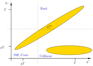
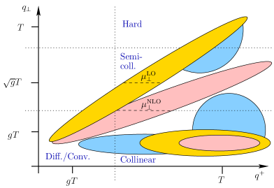
Figure 4: Left: kinematic regions, in terms of exchanged transverse momentum and exchanged light-cone momentum $q^{+}$, which are relevant at leading order. Right: the same regions (yellow) plus regions which are relevant at next-to-leading order (pink) and where subtractions of leading-order effects are needed (blue).

The relevant kinematics are summarized in Figure 4. Collinear processes correspond to a particle making a large change in energy but a small change in transverse momentum. Elastic scattering is a large change in both – or, for soft processes, a small change in both. The semi-collinear region is where the exchanged transverse momentum is intermediate between these two cases. Therefore it requires subtractions from each. It also requires a subtraction of its soft-exchange tail. We implement this as a cutoff on $q_{\perp}$ at the scale $\mu_{\perp}^{\mathrm{NLO}}$, but physically one could also see this as a way to cut off small energy (really $q^{+}$) exchanges.

To understand this region better, consider Eq. (23) and Eq. (24). In deriving the equation we assumed that $p,k\sim T$ and $\mathbf{h}\sim gT^{2}$. This allowed a collinear expansion; in particular we could equate $q_{\parallel}=\omega$ in exchange processes ($q^{-}=0$). But this breaks down as we consider larger $\mathbf{h}$ values. Fortunately in this regime there is a new simplifying approximation; the integral equation, Eq. (24), can be solved iteratively in large $\delta E$:

$$\mathbf{F}_{b1}(\mathbf{h}) =2\mathbf{h}/i\delta E(\mathbf{h})\,,$$ (70)

$$\mathbf{F}_{b2}(\mathbf{h}) =\frac{i}{\delta E(\mathbf{h})}\int\frac{d^{2}q_{\perp}}{(2\pi)^{2}}\bar{C}(q_{\perp})\left\{\left(C_{R_{b}}-\frac{C_{A}}{2}\right)[\mathbf{F}_{b1}(\mathbf{h})-\mathbf{F}_{b1}(\mathbf{h}-k\mathbf{q}_{\perp})]\right.$$

$$\quad\left.{}+\frac{C_{A}}{2}[\mathbf{F}_{b1}(\mathbf{h})-\mathbf{F}_{b1}(\mathbf{h}+p\mathbf{q}_{\perp})]+\frac{C_{A}}{2}[\mathbf{F}_{b1}(\mathbf{h})-\mathbf{F}_{b1}(\mathbf{h}-(p{-}k)\mathbf{q}_{\perp})]\right\}.$$

This is the same as treating the emission in the Bethe-Heitler limit, ignoring LPM corrections. We will make this approximation in the following. We can also assume that the $\mathbf{h}^{2}$ term dominates in the expression for $\delta E$, Eq. (26), so $\delta E(\mathbf{h})=h^{2}/(2pk(p{-}k))$.

However, as noted above, it is no longer sufficient to neglect $q^{-}$ relative to $q_{\perp}$, because $q^{-}=\delta E\sim gT\sim q_{\perp}$. Therefore the kinematics of scattering is changed and $\bar{C}(q_{\perp})$ must be recomputed. A more accurate form for $\bar{C}(q_{\perp})$ in this regime, replacing Eq. (25), is Ghiglieri:2013gia ; Ghiglieri:2015ala

$$\bar{C}_{\mathrm{NLO}}(q_{\perp},\delta E)=\frac{g^{2}Tm_{\scriptscriptstyle D}^{2}}{(q_{\perp}^{2}+\delta E^{2})(q_{\perp}^{2}+\delta E^{2}+m_{\scriptscriptstyle D}^{2})}+\frac{2g^{2}T\delta E^{2}}{q_{\perp}^{2}(q_{\perp}^{2}+\delta E^{2})}\,.$$ (71)

Physically this arises from two types of processes, in which the splitting is either induced by an elastic scattering or by the absorption of a soft on-shell particle, see Figure 5.

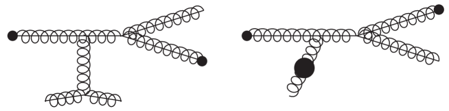
Figure 5: Diagrams for typical semi-collinear processes. The exchange of momentum $\mathbf{h}/p$ and energy with the plasma can be due to elastic scattering or absorption of a soft quasiparticle, leading to the semi-collinear splitting process.

Therefore we need to make two subtractions, corresponding to the already-computed LO ${1\leftrightarrow 2}$ contribution (the small $\delta E$ limit), and the already-included LO ${2\leftrightarrow 2}$ contribution (the small $m_{\scriptscriptstyle D}$ limit) Ghiglieri:2013gia :

$$\delta\bar{C}(q_{\perp},\delta E)=\frac{g^{2}Tm_{\scriptscriptstyle D}^{2}}{(q_{\perp}^{2}+\delta E^{2})(q_{\perp}^{2}+\delta E^{2}+m_{\scriptscriptstyle D}^{2})}-\frac{g^{2}Tm_{\scriptscriptstyle D}^{2}}{q_{\perp}^{2}(q_{\perp}^{2}+m_{\scriptscriptstyle D}^{2})}\,.$$ (72)

The second term is the LO collinear form for $\bar{C}$ (the small $\delta E$ limit of Eq. (71)). The other subtraction, of the $m_{\scriptscriptstyle D}\to 0$ limit, precisely removed the second term appearing in Eq. (71).

The semi-collinear contribution is found by substituting Eq. (72) into Eq. (70) and using it to evaluate Eq. (23) and hence Eq. (22). But one further simplification can be made. For generic $p,k\sim T$, we have $\delta E\sim h^{2}/T^{3}$. The two terms in Eq. (72) cancel up to small corrections unless $\delta E\sim m_{\scriptscriptstyle D}\sim gT$, which then requires the semi-collinear value $h\sim T^{2}\sqrt{g}$. On the other hand, $q_{\perp}\sim gT$; for larger values, $q_{\perp}^{2}\gg\delta E^{2}$ and the two terms again cancel. Therefore, we can make a systematic expansion in $p\mathbf{q}_{\perp}\ll\mathbf{h}$ in Eq. (70). And to get a strict NLO result, we also need to make such an expansion. Averaging over directions for $\mathbf{q}_{\perp}$, we have

$$\mathbf{F}_{b1}(\mathbf{h})-\mathbf{F}_{b1}(\mathbf{h}-p\mathbf{q}_{\perp})\simeq-\frac{p^{2}q_{\perp}^{2}}{4}\nabla_{\mathbf{h}}^{2}\mathbf{F}_{b1}(\mathbf{h})\,,$$ (73)

which we combine with the definition (see footnote 5)

$$\delta\bar{\hat{q}}(\delta E)\equiv\int\frac{d^{2}q_{\perp}}{(2\pi)^{2}}\>q_{\perp}^{2}\>\delta\bar{C}(q_{\perp},\delta E)$$ (74)

to get an explicit expression for $\mathbf{F}_{b2}(\mathbf{h})$, leading to Ghiglieri:2015ala

$$\gamma^{a}_{bc}\bigg{|}_{\mathrm{semi}}^{\mathrm{strict}}(p;p{-}k,k) =\frac{g^{2}}{8\pi^{4}}\left\{\begin{array}[]{cc}2d_{A}C_{A}^{2}\frac{(p^{2}+k^{2}-pk)^{3}}{pk(p-k)}&g\leftrightarrow gg\\ d_{F}C_{F}\frac{p^{2}+(p-k)^{2}}{k}[C_{F}k^{2}+C_{A}p(p-k)]&q\leftrightarrow qg\\ d_{F}C_{F}\frac{(p-k)^{2}+k^{2}}{p}[C_{F}p^{2}-C_{A}k(p-k)]&g\leftrightarrow q\bar{q}\end{array}\right\}$$ (78)

$$\quad{}\times\int\frac{d^{2}h}{(2\pi)^{2}}\frac{\delta\bar{\hat{q}}(\delta E_{s})}{h^{4}}.$$ (79)

When this result is inserted into Eq. (22) it leads to logarithmic small $k$ and $(p{-}k)$ divergences unless we impose an IR cutoff on the allowed value of $\mathbf{h}$, namely $\mathbf{h}\geq p\mu_{\perp}^{\mathrm{NLO}}$. The cutoff dependence cancels that in the NLO longitudinal momentum and identity change rates Ghiglieri:2015ala .

The problem with this procedure is the same as the problem with the strict LO rate. We need to insert a regulator scale which separates regions with finite $k$-momentum exchange from regions which are treated diffusively. Neither side is necessarily positive and the collision operator can have serious positivity problems when the coupling is not small. This necessitates a rewriting of the NLO contributions along the lines of the AMY method at LO. The problem arises because we made a strict $\mathbf{h}\gg p\mathbf{q}_{\perp}$ expansion in Eq. (73). Without this approximation, that is, by using the full expression for $\delta\bar{C}$, Eq. (72), in Eq. (70), we obtain instead the manifestly finite result

$$\gamma^{a}_{bc}\bigg{|}_{\mathrm{semi}}(p;p-k,k) =\frac{g^{2}}{32\pi^{4}}\left\{\begin{array}[]{cc}d_{A}C_{A}\frac{p^{4}+k^{4}+(p-k)^{4}}{p^{3}k^{3}(p-k)^{3}}&g\leftrightarrow gg\\ d_{F}C_{F}\frac{p^{2}+(p-k)^{2}}{p^{2}(p-k)^{2}k^{3}}&q\leftrightarrow qg\\ d_{F}C_{F}\frac{(p-k)^{2}+k^{2}}{(p-k)^{2}k^{2}p^{3}}&g\leftrightarrow q\bar{q}\end{array}\right.\int\frac{d^{2}h}{(2\pi)^{2}}\int\frac{d^{2}q_{\perp}}{(2\pi)^{2}}\delta\bar{C}(q_{\perp},\delta E)$$ (83)

$$\times\left[\left(C_{R}-\frac{C_{A}}{2}\right)\left(\frac{\mathbf{h}}{\delta E(\mathbf{h})}-\frac{\mathbf{h}-k\mathbf{q}_{\perp}}{\delta E(\mathbf{h}-k\mathbf{q}_{\perp})}\right)^{2}+\frac{C_{A}}{2}\left(\frac{\mathbf{h}}{\delta E(\mathbf{h})}-\frac{\mathbf{h}+p\mathbf{q}_{\perp}}{\delta E(\mathbf{h}+p\mathbf{q}_{\perp})}\right)^{2}\right.$$

$$\left.+\frac{C_{A}}{2}\left(\frac{\mathbf{h}}{\delta E(\mathbf{h})}-\frac{\mathbf{h}-(p-k)\mathbf{q}_{\perp}}{\delta E(\mathbf{h}-(p-k)\mathbf{q}_{\perp})}\right)^{2}\right],$$ (84)

with $(C_{R}-C_{A}/2)$ appearing on the $\mathbf{h}+p\mathbf{q}_{\perp}$ term for $g\leftrightarrow q\bar{q}$ processes. This is then inserted into Eq. (22), resulting in

$$\left(f_{1},\mathcal{C}^{\mathrm{semi}}f_{1}\right) \equiv \frac{2\pi}{T^{3}}\sum_{abc}\int_{0}^{\infty}\!\!dp\int_{0}^{p}dk\,\gamma^{a}_{bc}\bigg{|}_{\mathrm{semi}}\!\!(p;p-k,k)f^{a}_{0}(p)[1\pm f^{b}_{0}(k)][1\pm f^{c}_{0}(p-k)]$$ (85)

$$\times\left[f_{1}^{a}({\bm{p}})-f_{1}^{b}(k\hat{\bm{p}})-f_{1}^{c}((p-k)\hat{\bm{p}})\right]^{2}.$$

In the small $g$ limit, this single expression reduces to the sum of the previous NLO semi-collinear, $\delta\hat{q}_{\scriptscriptstyle L}$, and $\delta\Gamma^{\mathrm{conv}}$ contributions, as we show at some length in Appendix C. The appendix also explains how this result is related to the light-cone sum rules.

We conclude the illustration of this region with a remark. Currently, we treat the collinear region with Eq. (22) and the semi-collinear region, including a subtraction due to the collinear one, using Eq. (85). But we could combine them into a single calculation by adding $\delta\bar{C}(q_{\perp},\delta E)$ to $\bar{C}(q_{\perp})$ in Eq. (24). In this way one would perform LPM resummation with the $\delta E$-dependent kernel and thus would no longer need to subtract the strictly collinear one. The contribution would also be manifestly positive. However, this would be extremely impractical. Because $\bar{C}(q_{\perp})$ is quite simple, we can Fourier transform it analytically and solve Eq. (24) in impact-parameter space as a differential equation. But $\delta\bar{C}$ does not have a simple Fourier expression, so Eq. (24) would need to be solved as an integral equation in $\mathbf{q}_{\perp}$ space, making a numerical solution very intricate. Treating the parts separately as we do, with the expansion Eq. (70) used for the semi-collinear but not the collinear case, does not lead to a manifestly positive result. But the sum nevertheless tends to remain positive, even for large $m_{\scriptscriptstyle D}/T$, because $\delta\bar{C}(q_{\perp},\delta E)$ becomes smaller in that limit.

4.4 Estimate of NLO gain terms

We have now presented the NLO contributions except for possible gain terms, as explained in Section 3. Although we will not be able to compute these, we can at least estimate their size, which allows us to assign a systematic error budget for their exclusion. NLO effects arise from soft momenta and from corrections to collinear and semi-collinear physics. For the latter, a small momentum exchange induces a large change in the particle which splits, and since we capture all aspects of this large change, only the soft exchange partner is mistreated. This is a subleading effect. Therefore we only need concern ourselves about NLO gain terms due to momentum diffusion and identity change.

To get an estimate for their magnitude, we compute the soft contribution from gain terms in the LO calculation, where we know how to compute and include them. Then we estimate that the missing NLO gain terms are of order the same size, times a factor reflecting how much smaller NLO effects are relative to the leading order. In the $\ell=2$ case, where, as we’ve seen in the previous section, gain terms are only mediated by soft gluon exchange, we shall use

$$\Big{(}\chi_{ij},{\cal C}^{\delta\mathrm{gain}}\,\chi_{ij}\Big{)}=C_{\ell=2}\frac{m_{\scriptscriptstyle D}}{T}\left.\Big{(}\chi_{ij},{\cal C}^{2\leftrightarrow 2}_{\mathrm{diff}}\chi_{ij}\Big{)}\right|_{\rm gain},$$ (86)

where $C_{\ell=2}$ is a constant that we vary to incorporate our ignorance of the actual size (and sign!) of the NLO gain terms. We are thus making the Ansatz that the NLO corrections to the gain terms take the exact same form as at leading order, but rescaled by $m_{\scriptscriptstyle D}/T\sim g$ times an arbitrary constant. Similarly, for the $\ell=1$ case, where only fermionic gain terms contribute, we assume

$$\Big{(}\chi_{i},{\cal C}^{\delta\mathrm{gain}}\,\chi_{i}\Big{)}=C_{\ell=1}\frac{m_{\scriptscriptstyle D}}{T}\left.\Big{(}\chi_{i},{\cal C}^{2\leftrightarrow 2}_{\mathrm{conv}}\,\chi_{i}\Big{)}\right|_{\rm gain}.$$ (87)

We evaluate each expression, as given in Eqs. (41) and (58), in Appendix B.2. Our results will show that the impact of these gain terms is very modest.

4.5 Summary

We conclude this section by summarizing the form of the collisional part of the quadratic functional. At LO it is given by Eq. (20). At NLO we have

$$\Big{(}f_{1},{\cal C}_{\mathrm{NLO}}\,f_{1}\Big{)}{}=\Big{(}f_{1},{\cal C}_{\mathrm{LO}}\,f_{1}\Big{)}+\Big{(}f_{1},\delta{\cal C}\,f_{1}\Big{)}\,,$$ (88)

where

$$\Big{(}f_{1},\delta{\cal C}\,f_{1}\Big{)}\equiv \Big{(}f_{1},{\cal C}^{\delta\hat{q}}\,f_{1}\Big{)}-\Big{(}f_{1},{\cal C}^{2\leftrightarrow 2}_{\mathcal{O}(g)\,\mathrm{finite}}\,f_{1}\Big{)}+\Big{(}f_{1},{\cal C}^{\delta\mathrm{gain}}\,f_{1}\Big{)}$$ (89)

$$+\Big{(}f_{1},{\cal C}^{\mathrm{semi}}\,f_{1}\Big{)}+\Big{(}f_{1},\delta{\cal C}^{{1\leftrightarrow 2}}\,f_{1}\Big{)}.$$ (90)

Here the first contribution is found by inserting $\delta\hat{q}^{a}$ from Eq. (63) in place of $\hat{q}^{a}$ in Eq. (40). In the form most suited for numerical evaluation it reads

$$\Big{(}\chi_{i\cdots j},{\cal C}^{\delta\hat{q}}\,\chi_{i\cdots j}\Big{)}=\frac{\beta^{3}}{2}\sum_{a}\nu_{a}\,\delta\hat{q}^{a}\int_{\bm{p}}f^{a}_{0}(p)[1\pm f_{0}^{a}(p)]\frac{\ell(\ell+1)\chi^{a}(p)^{2}}{2p^{2}}.$$ (91)

The second term in Eq. (89) is the “counterterms” discussed in Subsection 4.2 and computed in Appendix B.3, the third is the estimate in Eq. (86) or Eq. (87), the fourth is from Eq. (85), and the last is the result of the modification of Eq. (66), inserted in Eq. (22).

5 Results

As we have mentioned in Sec. 2, we obtain the leading-order transport coefficients by maximizing the functional $\mathcal{Q}[\chi]$, as given by Eq. (16), with the source term given in Eq. (19) and the LO collision operator given in Eq. (20), with modifications described in Subsection 4.2, especially Eq. (69). In the previous section we have derived the NLO collision operator, as summarized in Eq. (88). This operator is the sum of the LO one and of its $\mathcal{O}(g)$ corrections. In principle, one could treat the latter as a perturbation. One extremizes Eq. (16) by series expanding $1/({\cal C}+\delta{\cal C})$ as a geometric series,

$$\beta^{4}\mathcal{Q}_{\mathrm{max}}=\Big{(}{\cal S},\frac{1}{{\cal C}+\delta{\cal C}}\,{\cal S}\Big{)}\;\Longrightarrow\;\Big{(}{\cal S},\frac{1}{{\cal C}}\,{\cal S}\Big{)}-\Big{(}{\cal S},\frac{1}{{\cal C}}\,\delta{\cal C}\,\frac{1}{{\cal C}}\,{\cal S}\Big{)}+\ldots\,.$$ (92)

We have however chosen not to pursue this avenue because $\delta{\cal C}$ can be large and positive, and the above expression becomes negative for intermediate $g$ values. Hence, we instead define the NLO transport coefficients as the expression before the $\Longrightarrow$ in Eq. (92), rather than the expression after the arrow. One way to think of this is that we are computing $1/\eta$ at NLO and then inverting it, similar to resumming self-energy insertions into a Dyson sum so they appear linearly in the denominator of the propagator.

We will plot the ratio $\eta/s$ using the leading-order, Stephan-Boltzmann value for the entropy density with $N_{f}$ massless quarks, since the first perturbative corrections to the partition function, from which all thermodynamic observables are obtained, are of order $g^{2}$. This is self-consistent within our kinetic approach, and to do otherwise would be treating particles’ contribution to the entropy and to the stress tensor differently and inconsistently.

We will start by presenting results in full QCD with fermions. Later on, in Sec. 5.2, we will also present results for the pure Yang-Mills theory and in Sec. 5.3 for QED. Accurate fits for the NLO results will be presented in App. D.

5.1 Results in full QCD

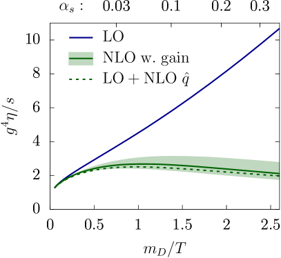
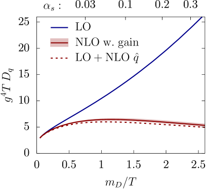
Figure 6: (a) The shear viscosity to entropy ratio $\eta/s$, and (b) the baryon number diffusion coefficient $D_{q}$ (times temperature) normalized by the leading $1/g^{4}$ as a function of $m_{\scriptscriptstyle D}/T$ for QCD with $N_{f}=3$ light flavors. (The corresponding value of $\alpha_{\mathrm{s}}$ is shown on the upper horizontal axis.) The LO result is from Arnold:2003zc . The uncertainty from the unknown gain terms is shown by the bands; it is estimated from the leading-order gain terms (which have the same structure as their NLO counterparts) by changing an unknown coefficient $C_{\ell}$ through the range $[-2,2]$ as specified by Eq. (86) and Eq. (87). The dashed lines represent an estimate in which we include only the NLO $\hat{q}$ to the LO collision operator – see Eq. (93) and surrounding text.

In Fig. 6 we show our results for the shear viscosity over entropy $\eta/s$ and quark number diffusion $D_{q}$ as a function of $m_{\scriptscriptstyle D}/T$ for QCD with $N_{f}=3$ flavors. We plot the LO results Arnold:2003zc in solid blue, and for NLO we plot our result in solid green (for $\eta/s$) and red (for $D_{q}$). To estimate the uncertainty from the undetermined NLO gain terms we provide bands in the same color around these central $C_{\ell}=0$ NLO values. The bands are obtained from taking $C_{\ell}$ in the range $[-2,2]$. This apparently arbitrary choice is motivated by comparing LO and NLO momentum diffusion rates; the NLO $\hat{q}$ to LO $\hat{q}$ ratio is $\delta\hat{q}^{a}/(\hat{q}^{a}m_{\scriptscriptstyle D}/T/\ln(\mu_{\perp}/m_{\scriptscriptstyle D}))$, which we can read off from Eqs. (39) and (63); it ranges from $\sim 1$ for $N_{f}=6$ to $\sim 2.2$ in the pure Yang-Mills case. Therefore $|C_{\ell}|=2$ appears to be a conservative value in estimating resulting errors. As we point out in App. B.2, we have made another conservative choice there in the evaluation of the gain terms. The uncertainty arising from the gain terms is smaller for $D_{q}$ than for the shear viscosity; in the former case we are dealing with the soft-fermion, $\ell=1$ term given by Eq. (87), whose LO value (Eqs. (58) and (108)) is numerically smaller than its $\ell=2$ counterpart (Eqs. (41) and (42)).

In both cases the main difference between LO and NLO results arises from $\delta\hat{q}$. This is reinforced by the dashed lines in Fig. 6, which shows results obtained from a collision operator containing, beyond leading order, only the NLO corrections to $\hat{q}$:

$$\Big{(}f_{1},{\cal C}^{\delta\hat{q}}_{\mathrm{only}}\,f_{1}\Big{)}\equiv\Big{(}f_{1},{\cal C}_{\mathrm{LO}}\,f_{1}\Big{)}+\Big{(}f_{1},{\cal C}^{\delta\hat{q}}\,f_{1}\Big{)}-\Big{(}f_{1},{\cal C}^{2\leftrightarrow 2}_{\mathcal{O}(g)\,\mathrm{finite}\,\hat{q}}\,f_{1}\Big{)}\,,$$ (93)

with the pertinent “counterterm” $(f_{1},{\cal C}^{2\leftrightarrow 2}_{\mathcal{O}(g)\,\mathrm{finite}\,\hat{q}}\,f_{1})$ given by Eq. (118). We see that this curve lies quite close to the ($C_{\ell}=0$) full NLO result, indicating that other corrections are small or largely cancel each other. But the $\delta\hat{q}$ contribution is so large that it starts to overtake the leading-order collision operator before $m_{\scriptscriptstyle D}=1T$ and represents a factor-5 modification for $\alpha_{\mathrm{s}}=0.3$. We present an accurate fit for the NLO curves (at $C_{\ell}=0$) in App. D, namely in Eqs. (150) and (151) for $\eta/s$ and in Eqs. (153) and (154) for $D_{q}$.

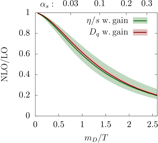
Figure 7: The NLO/LO ratio for the shear viscosity and diffusion constant for QCD with $N_{f}=3$. The uncertainty bands from the unknown gain terms are described in Fig. 6.

In order to study more quantitatively the observed similar trend between the NLO $\eta$ and $D_{q}$, compared to their respective leading orders, we plot the NLO/LO ratios in Fig. 7, complete with gain uncertainty bands, as a function of $m_{\scriptscriptstyle D}/T$ for QCD with $N_{f}=3$. As the plot shows, the two central values fall within the uncertainty bands. Each transport coefficient is dominated by elastic scattering and in each case the ratio of $\delta\hat{q}$ to the leading-order elastic effect is about the same; therefore the trend with coupling is very similar.

True vacuum renormalization effects will first arrive at NNLO (at $\mathcal{O}(g^{2})$), so we do not yet see effects of coupling renormalization. This makes it difficult to use any internal consistency to set the scale in our calculations. Nevertheless, we are clearly very interested in plotting the temperature dependence of the LO and NLO transport coefficients, which requires picking a prescription for $g(T)$ and for the quark mass thresholds, with the understanding that the different choices might differ starting parametrically from NNLO. Various choices are commonly employed in the literature. One widely used prescription is to simply take the $\overline{\mathrm{MS}}$ coupling at $n$ loops, with threshold matching at $n-1$ loops, and choose the renormalization scale $\mu$ to be a multiple of the Matsubara frequency $2\pi T$ (usually a set of values such as $\mu=\{0.5,1,2,4\}\pi T$ is employed to estimate the scale setting uncertainty). Another choice is to use the “effective QCD coupling”, introduced in Laine:2005ai as the matching coefficient appearing in the dimensionally reduced effective theory EQCD (Electrostatic QCD, Braaten:1994na ; Braaten:1995cm ; Braaten:1995jr ; Kajantie:1995dw ; Kajantie:1997tt ). The two-loop expression for this matching coefficient, as computed in Laine:2005ai , is better suited to describe the coupling in settings where contributions from the soft scales play a major role, as the computation of the spatial string tension and comparison with lattice data in Laine:2005ai display. Since the LO results are dominated by the logarithmically enhanced diffusion and conversion processes Arnold:2003zc , which are very sensitive to the soft scale, and the NLO results are dominated by the large corrections to $\hat{q}$, which are in turn determined from EQCD, we argue that the EQCD coupling is the best choice for these transport coefficients. Hence we will mostly use the EQCD coupling from Laine:2005ai in our plots.

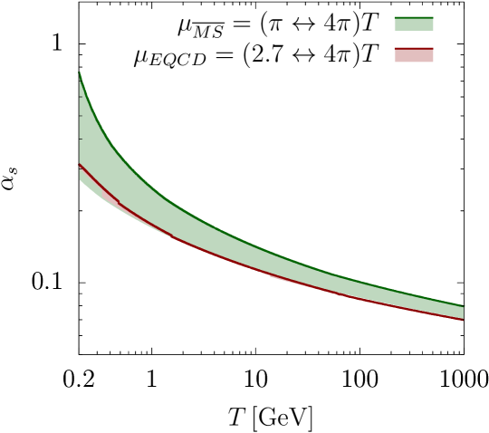
Figure 8: The different choices for the coupling as a function of the temperature adopted in this work. The green band (and bounding line) is obtained from a two-loop QCD ${\overline{\rm MS}}$ running with one-loop threshold matching (and hence is continuous at the thresholds) with $\mu_{\overline{MS}}=(\pi\leftrightarrow 4\pi)T$. The green bounding line is for the smallest scale $\mu_{\overline{MS}}=\pi T$. The corresponding red band and bounding line are obtained from the EQCD effective coupling with $\mu_{EQCD}=(2.7\leftrightarrow 4\pi)\,T$ Laine:2005ai , which is discontinuous at the quark thresholds.

We start by plotting the coupling itself, as shown in Fig. 8. The detailed definitions for the two choices of the coupling are given in App. E. The green line and band represent the QCD ${\overline{\rm MS}}$ coupling as given by Eq. (155), obtained from a numerical two-loop evolution from $\alpha_{\mathrm{s}}(M_{z})=0.1185$, with the $\overline{\mathrm{MS}}$ renormalization scale $\mu$ in the range $[\pi T,4\pi T]$ and with one-loop quark threshold matching at $\mu=m_{q}$, hence the continuity. The red line and band are instead obtained from the effective EQCD coupling, as given by Eq. (158), with threshold matching at $\mu=m_{q}$ and with renormalization scale $\mu$ in the range $[2.7T,4\pi T]$. The lower bound ($\mu=2.7T$) is at the quark mass value ($m_{q}=2.7T$) where a quark contributes half as much (Stephan-Boltzmann) entropy as a massless quark, which we therefore pick as our criterion for the quark’s decoupling temperature (for instance, the $b$ quark decouples at $T_{b}\approx 1.55$ GeV under this choice). As we remark in App. E, the matching to the EQCD coupling cancels the leading renormalization point dependence, which is why the EQCD curves are nearly identical.

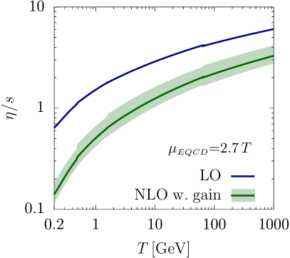
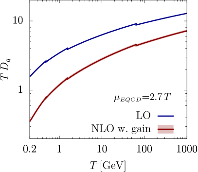
Figure 9: (a) The QCD shear viscosity to entropy density ratio $\eta/s$, and (b) diffusion coefficient $D_{q}$ as a function of $T$. All curves in this plot are obtained using the effective EQCD coupling with $\mu_{EQCD}=2.7\,T$. The uncertainty due to the gain terms which are estimated (and not computed) is shown by the shaded green and red bands respectively. This uncertainty estimate is described in Fig. 6.

Fig. 9 shows the LO (blue) and NLO results for $\eta/s$ (green) and $D_{q}$ (red) with the effective EQCD coupling, set at the entropy-motivated prescription $\mu=2.7T$. At the quark mass thresholds we switch from describing a system with $N_{f}+1$ massless quark flavors to describing a system with $N_{f}$ massless flavors, leading to a discontinuity in the coupling, the entropy density and the transport coefficients, and therefore in each curve. Our treatment is insufficient near each threshold because we have not developed an $\eta$ (or $D_{q}$) calculation which correctly treats massive quarks. We show the uncertainty bands corresponding to the previous values for the arbitrary constant in Eq. (86): $C_{\ell}=\pm 2$. As the plot shows, in the $\eta/s$ case the uncertainty band due to missing NLO (gain) contributions grows larger as $N_{f}$ increases with increasing temperature. This is because the LO gain term, which multiplies $C_{\ell=2}$ in Eq. (86), has terms proportional to $N_{f}$ and to $N_{f}^{2}$, as can be inferred from Eq. (41). We remark that, as expected from Fig. 6, the NLO results are much smaller than the leading order: at temperatures of the order of the QCD transition the NLO $\eta/s$ is smaller by a factor of 5, which becomes a factor of two for $T\sim 1$ TeV. The gain uncertainty band, on the other hand, represents a $+30\%$, $-20\%$ correction to the NLO result. In terms of the strong-coupling results Policastro:2001yc ; Policastro:2002se ; CaronHuot:2006te , the NLO results for $\eta/s$ ($D_{q}$) can get smaller than $2/(4\pi)$ ($2/(2\pi T)$) at the lowest temperatures, corresponding to couplings of the order of $\alpha_{\mathrm{s}}\sim 0.35$.

In Fig. 1 we analyzed another source of theoretical uncertainty, arising from a different scheme for the running coupling. Besides the LO and NLO results with the EQCD effective coupling, already presented in Fig. 9, we also show results obtained from the two-loop QCD ${\overline{\rm MS}}$ coupling discussed above. As the plot shows, the LO and NLO uncertainty bands introduced by the different choices adopted for the renormalization scale are well separated (except at the lowest temperatures, where, as Fig. 8 shows, the ${\overline{\rm MS}}$ coupling for $\mu=\pi T$ is $\mathcal{O}(1)$). This is consistent with the expectation that the running coupling is an NNLO effect and should thus be smaller than NLO corrections.

5.2 Results in pure Yang-Mills

Pure Yang-Mills theory is only of interest for academic reasons. Nevertheless, since it is straightforward, and since most lattice results for the viscosity Nakamura:2004sy ; Meyer:2007ic ; Astrakhantsev:2015jta ; Astrakhantsev:2017nrs ; Mages:2015rea ; Pasztor:2016wxq ; Pasztor:2018yae , as well as analytical studies Keegan:2015avk , are actually for pure Yang-Mills theory and not full QCD, we will present results for this case.

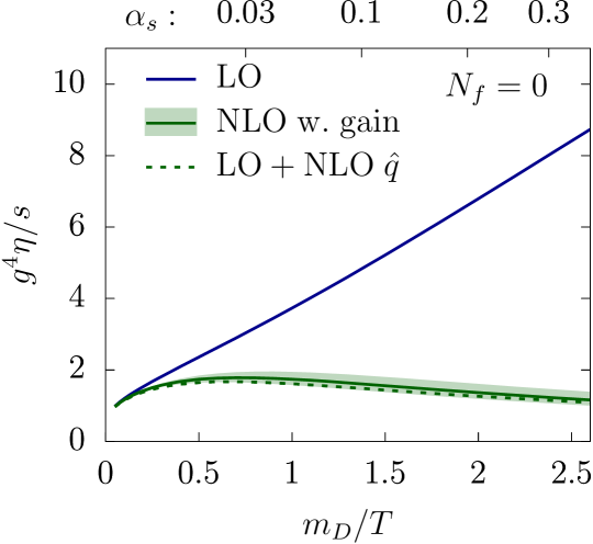
Figure 10: The $\eta/s$ ratio in units of $1/g^{4}$ as a function of $m_{\scriptscriptstyle D}/T$ for $N_{c}=3$ Yang-Mills theory. The uncertainty band is due to the unknown gain terms described in Fig. 6. A fit for the solid green curve is available in Eqs. (150) and (152). The dashed line shows a partial NLO result with only the NLO modifications to $\hat{q}$.

In Fig. 10 we show the $\eta/s$ ratio in pure Yang Mills for $N_{c}=3$. The general trends are the same as in full QCD but, interestingly, the NLO/LO ratio is smaller as a function of $m_{\scriptscriptstyle D}/T$ than it is for full QCD. When examined in terms of $g$ (see the upper scale in $\alpha_{\mathrm{s}}$) they are however similar. It is also worth noting that the absolute values for $\eta/s$ are larger than for $N_{f}=3$.

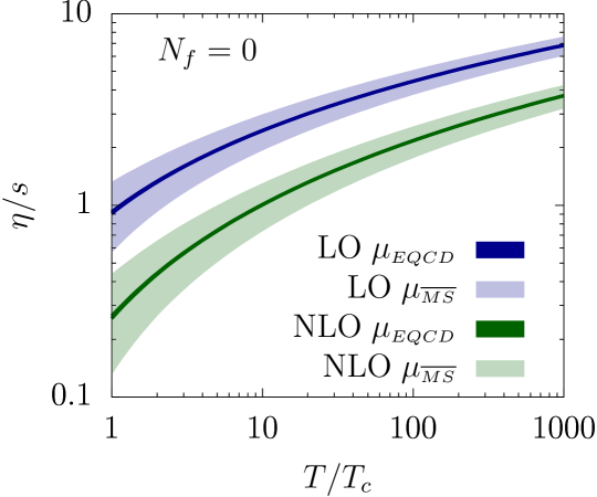
Figure 11: The $\eta/s$ ratio as a function of the temperature for $N_{c}=3$, $N_{f}=0$ pure Yang-Mills theory. The thin darker bands and the thicker lighter bands respectively show the EQCD and $\overline{MS}$ renormalization schemes with $\mu=(\pi\leftrightarrow 4\pi)T$.

In Fig. 11 we plot the $\eta/s$ ratio in $N_{c}=3$ Yang-Mills theory as a function of the temperature. The coupling is fixed as follows:

• At a sufficiently high scale we impose the two-loop asymptotics $\alpha_{\mathrm{s}}(\mu)/\pi=-8/(\beta_{0}t)-16\beta_{1}\ln(t)/(\beta_{0}^{3}t^{2})$, with $t=\ln(\mu^{2}/\Lambda^{2}_{\overline{\mathrm{MS}}})$, $\beta_{i}$ as given by Eq. (157) and $\Lambda_{\overline{\mathrm{MS}}}=1.24T_{c}$ Francis:2015lha , with $T_{c}$ the critical temperature.

• For the two-loop QCD ${\overline{\rm MS}}$ coupling, this asymptotic value is then evolved down to lower scales using the two-loop $\beta$-function in Eq. (155). We present LO and NLO results as wide blue and green bands respectively, reflecting the renormalization scale uncertainty. Uncertainties arising from the $\Lambda_{\overline{\mathrm{MS}}}/T_{c}$ ratio or from the two-loop truncation of the $\beta$-function should be smaller than the large bands arising from the variation of the renormalization scale.

• For the effective EQCD coupling we use Eq. (158) as before. The displayed darker blue (LO) and green (NLO) bands, for the the same $\mu$ interval as in the ${\overline{\rm MS}}$ case, are much narrower, given that the dependence on $\mu$ is very small in the absence of the discontinuities at the quark mass thresholds.

In this case one observes again two non-overlapping bands for the LO and NLO shear viscosity. Due to the smaller values of the couplings the shear viscosity over entropy density is larger than in full QCD in the transition region.

5.3 Results in QED

We have also obtained the shear viscosity for QED. In this theory the large NLO $\hat{q}$ contribution is absent, due to its non-abelian nature, and the coupling is small. We have taken $\alpha=0.0072973525664$ and one massless Dirac fermion, so as to describe an electron-positron-photon plasma at $m_{\mu}\gg T\gg m_{e}$. In QED $m_{D}^{2}=e^{2}T^{2}/3$ and hence $m_{D}/T\approx 0.17$. At leading order we obtain

$$\frac{\eta}{s}\bigg{|}_{\mathrm{QED}}^{\mathrm{LO}}=2779.2,$$ (94)

whereas our next-to-leading order results, for three values of the gain constant $C_{\ell=2}$, are

$$\frac{\eta}{s}\bigg{|}_{\mathrm{QED}}^{\mathrm{NLO,\,C_{\ell=2}=0}}=2818.5,\qquad\frac{\eta}{s}\bigg{|}_{\mathrm{QED}}^{\mathrm{NLO,\,C_{\ell=2}=+2}}=2836.1,\qquad\frac{\eta}{s}\bigg{|}_{\mathrm{QED}}^{\mathrm{NLO,\,C_{\ell=2}=-2}}=2801.2.$$ (95)

Hence, the NLO central value ($C_{\ell=2}=0$) corresponds to a 1.4% increase over the LO shear viscosity, while the upper and lower values correspond to a 2% and a 0.8% increase respectively. We can thus conclude that the abelian NLO corrections tend to decrease the collision operator and that in the case of QED perturbation theory works very well.

6 Conclusions

The main aim of this paper has been to compute the shear viscosity and quark diffusion coefficient of QCD at “almost” NLO in $g$. This involved partially resumming some $\mathcal{O}(g)$ effects in the leading-order treatment, and some $\mathcal{O}(g^{2})$ effects in the NLO treatment, in order to maintain positivity of the collision operator. Also we invert the full ${\cal C}+\delta{\cal C}$ (leading plus next-to-leading order) collision operator, rather than expanding in $\delta{\cal C}$ as suggested in Eq. (92). It also involved neglecting gain terms which we could not compute at NLO, but which proved to be small at leading order. We have estimated the possible effects of these missing contributions and found they are likely quite small. From a technical standpoint, the most important result of this paper is the methodology introduced in Sec. 4.3, where we introduce a ${1\leftrightarrow 2}$ rate, Eq. (84), which smoothly extends into regions of soft or semi-collinear (less collinear) radiation, without the need for intermediate regulators. In this paper we have only needed to treat this new equation in the single-scattering (Bethe-Heitler) regime, but it would be interesting to try to solve it as an integral equation, thereby incorporating LPM interference when needed. We leave this, together with applications of this approach to thermalization or jet quenching, to future studies.

The qualitative trend observed for the shear viscosity and the light quark diffusion coefficients as a function of the coupling $m_{\scriptscriptstyle D}/T$, both in QCD with three light fermions and in the pure gauge theory, is as follows (see Figs. 6, 7, 10): the NLO curves in green ($\eta/s$) or red ($D_{q}$) start to diverge significantly from the LO ones in blue for $m_{\scriptscriptstyle D}/T\sim 0.5$, with the NLO transport coefficients becoming as small as one fifth of the LO for values of $m_{\scriptscriptstyle D}/T$ corresponding to $\alpha_{\mathrm{s}}\sim 0.3$. Furthermore, the uncertainty band introduced by considering a rather large value for the gain terms at NLO only modify the NLO transport coefficients by 30% at most. In Figs. 1, 9 and 11, we plot instead the transport coefficients as functions of the temperature, which requires picking a prescription for the coupling as a function of the temperature and for the decoupling of heavy quarks. The LO and NLO curves do not overlap, even accounting for the uncertainties arising from the choice of the running prescription, renormalization scale and decoupling point. Therefore the limitations of perturbation theory are much more severe than simply the question of what to choose for the renormalization point. Indeed, even at temperatures of order one TeV, where perturbation theory would be expected to work well, the NLO transport coefficients are smaller than the LO value by about a factor of 2.

The dashed curves in Figs. 6 and 10 show that by far the dominant NLO effect is the large NLO correction to $\hat{q}$, first derived in Ref. CaronHuot:2008ni . This should perhaps not be too surprising. The corrections to splitting rates are not small, but they tend to be compensated by the semi-collinear ones Ghiglieri:2013gia . And as emphasized in Arnold:2003zc , elastic scattering is the principal contributor to shear viscosity and number diffusion, with splitting processes amounting to 10–20% effects. Further, the NLO contributions to $\hat{q}$ represent new physical processes not included at leading order; the inclusion of additional soft emissions in the course of scattering and interference between different scattering processes. Unfortunately the Euclidean methods used to compute $\delta\hat{q}$ do not allow us to evaluate these contributions separately. In order to test a theory that is not sensitive to this large $\delta\hat{q}$ contribution, we examined QED in Sec. 5.3, finding that the remaining abelian NLO contributions are a percent-level correction.

One important question to be addressed is what should we make of a perturbative expansion that does not converge above $m_{\scriptscriptstyle D}/T\sim 0.5$, or equivalently below temperatures well above the TeV scale. Taken at face value, the results plotted in Sec. 5 would perhaps suggest a grim answer to this question. However, one could optimistically think that, if we were to correctly identify the physics responsible for these large corrections, and rearrange the perturbative expansion by resumming it, possibly in the form of an Effective Field Theory, then the outlook on convergence would be quite different; a redefined LO somehow incorporating most of the NLO corrections to $\hat{q}$ would not look so different from the dashed lines in Fig. 6, so that the deviation from the NLO in solid green/red would be much less pronounced. Of course, much action is needed to move this scenario from the realm of wishful thinking into physically motivated perturbative schemes. One possible direction would be to treat the problematic soft sector non-perturbatively. The mapping to the Euclidean 3D theory makes a lattice determination of the soft contribution to $\mathcal{C}(q_{\perp})$ and $\hat{q}$ possible, with first results reported in Panero:2013pla . Refinements of this measurement, together with calculations of the shift in the dispersion relation $\delta m_{\infty}^{2}$ and of $\hat{q}(\delta E)$, seem within reach, due to their Euclidean nature. We also need a better understanding of how such Euclidean measurements can be systematically included into transport calculations within a rigorous Effective Field Theory framework. Other needed ingredients, such as the longitudinal momentum broadening, conversion rates and gain terms, on the other hand, cannot be mapped to the 3D Euclidean theory and cannot thus be currently determined on the lattice. Therefore we should view it as good news that these effects appear to be much smaller than $\delta\hat{q}$. One might hope that, with enough nonperturbative Euclidean contributions, the perturbative approach might work down closer to experimentally realizable temperatures.

Appendix A Hard Thermal Loop propagators

In the next appendices we will look at matrix elements with soft exchange momenta in more detail. Therefore we need to specify the hard thermal loops, which appear in the expressions for these soft, screened matrix elements. We start with the fermionic HTLs, which are most easily written in terms of components with positive and negative chirality-to-helicity ratio. The retarded fermion propagator reads

$$S_{R}(P)=h^{+}_{\mathbf{p}}S^{+}_{R}(P)+h^{-}_{\mathbf{p}}S^{-}_{R}(P)\,,$$ (96)

where

$$S^{\pm}_{R}(P)=\frac{i}{p^{0}\mp(p+\Sigma^{\pm}(p^{0}/p))}=\left.\frac{i}{\displaystyle p^{0}\mp\left[p+\frac{m_{\infty}^{2}}{2p}\left(1-\frac{p^{0}\mp p}{2p}\ln\left(\frac{p^{0}+p}{p^{0}-p}\right)\right)\right]}\right|_{p^{0}=p^{0}+i\epsilon},$$ (97)

where the upper (lower) sign refers to the positive (negative) chirality-to-helicity component. The projectors are $h^{\pm}_{\mathbf{p}}\equiv(\gamma^{0}\mp\vec{\gamma}\cdot\hat{p})/2$. Here $m_{\infty}^{2}$ is the fermionic asymptotic mass squared, defined such that the large-momentum dispersion relation for helicity=chirality fermions is $p_{0}^{2}=p^{2}+m_{\infty}^{2}$. We similarly define the asymptotic gluonic mass $M_{\infty}^{2}$. At leading order, their values are

$$M_{\infty}^{2}=\frac{m_{\scriptscriptstyle D}^{2}}{2}=\frac{g^{2}T^{2}}{6}\left(N_{c}+\frac{N_{f}}{2}\right),\qquad m_{\infty}^{2}=2m_{q}^{2}=C_{F}\frac{g^{2}T^{2}}{4},$$ (98)

where we have also shown the relations to the more commonly used Debye mass $m_{\scriptscriptstyle D}$ and quark “mass” $m_{q}$.

Gluons are described in the strict Coulomb gauge by

$$G^{00}_{R}(Q) = \frac{i}{\displaystyle q^{2}+m_{\scriptscriptstyle D}^{2}\left(1-\frac{\omega}{2q}\ln\frac{\omega+q+i\epsilon}{\omega-q+i\epsilon}\right)},$$ (99)

$$G^{ij}_{R}(Q) = (\delta^{ij}-\hat{q}^{i}\hat{q}^{j})G^{T}_{R}(Q)=\left.\frac{i(\delta^{ij}-\hat{q}^{i}\hat{q}^{j})}{\displaystyle\omega^{2}-q^{2}-M_{\infty}^{2}\left(\frac{\omega^{2}}{q^{2}}-\left(\frac{\omega^{2}}{q^{2}}-1\right)\frac{\omega}{2q}\ln\frac{\omega{+}q}{\omega{-}q}\right)}\right|_{\omega=\omega+i\epsilon}.$$

Appendix B Gain terms and finite order-g subtractions in 2 to 2 processes

In this section we first provide some details on the phase space integration coordinates in Sec. B.1. We then evaluate numerically the gain terms at leading order in Sec. B.2. In Sec. B.3 we will instead address the $\mathcal{O}(g)$ contributions in the $2\leftrightarrow 2$ collision operator that need to be subtracted, i.e. $(\chi_{i\cdots j},{\cal C}^{2\leftrightarrow 2}_{\mathcal{O}(g)\,\mathrm{finite}}\,\chi_{i\cdots j})$ in Eq. (89).

B.1 Phase space

In Sec. 3.1 we provided the phase space integration in the soft approximation in Eq. (32). We now set out to briefly justify that equation and provide more elements for the evaluations that will be performed in Sec. B.2 and B.3. One starts by eliminating a variable through the three-momentum $\delta$-function,

$$\int_{PS}\equiv\int_{{\bm{p}}{\bm{k}}{\bm{p}}^{\prime}{\bm{k}}^{\prime}}(2\pi)^{4}\delta(P+K-P^{\prime}-K^{\prime})=\int_{{\bm{p}}{\bm{k}}{\bm{p}}^{\prime}}2\pi\delta(p+k-p^{\prime}-k^{\prime})\,.$$ (101)

In the $t$ channel, ${\bm{p}}^{\prime}$ can then be shifted to ${\bm{q}}={\bm{p}}^{\prime}-{\bm{p}}$ and an extra $\omega$ integral is introduced, i.e.

$$\int_{PS}=\int_{{\bm{p}}{\bm{k}}{\bm{q}}}\int d\omega\,2\pi\delta(p-p^{\prime}+\omega)\,\delta(k-k^{\prime}-\omega)\simeq\int_{{\bm{p}}{\bm{k}}}\int\frac{d^{4}Q}{(2\pi)^{4}}\,2\pi\delta(v_{\bm{p}}\cdot Q)\,2\pi\delta(v_{\bm{k}}\cdot Q)\,,$$ (102)

where we have introduced the four-vector $Q=(\omega,{\bm{q}})$ and expanded the arguments of the $\delta$-functions for $\omega,q\sim gT\ll p,k$, recovering Eq. (32). Using the coordinate parameterization of Arnold:2003zc , Eq. (102) becomes

$$\int_{PS}\bigg{|}_{\mathrm{soft}} =\frac{1}{32\pi^{6}}\int_{0}^{\infty}dp\,p^{2}\int_{0}^{\infty}dk\,k^{2}\int_{0}dq\int_{-q}^{q}d\omega\int_{0}^{2\pi}d\phi$$

$$=\frac{1}{32\pi^{6}}\int_{0}^{\infty}dp\,p^{2}\int_{0}^{\infty}dk\,k^{2}\int_{0}dq_{\perp}\,q_{\perp}\int_{-\infty}^{\infty}\frac{d\omega}{q}\int_{0}^{2\pi}d\phi\,,$$ (103)

where $\phi$ is the angle between the ${\bm{p}},{\bm{q}}$ and ${\bm{k}},{\bm{q}}$ planes and in going from the first to the second line we have used the change of variables discussed in footnote 2, with $q=\sqrt{\omega^{2}+q_{\perp}^{2}}$. For future convenience we recall that in these coordinates and in the soft approximation

$$\hat{\bm{p}}\cdot\hat{\bm{k}}=\frac{\omega^{2}}{q^{2}}+\left(1-\frac{\omega^{2}}{q^{2}}\right)\cos\phi\,.$$ (104)

B.2 LO gain terms

Let us begin with the gluon exchange contribution at leading order. We recall that it only contributes for $\ell=2$. Starting from Eq. (41) and Eq. (42), using the results in Sec. B.1 for the phase space and the $\hat{\bm{p}}\cdot\hat{\bm{k}}$ angle, as well as the explicit form of the propagators in App. A, we have for $c_{1}$

$$c_{1} =\int\frac{d\Omega_{{\bm{k}}}}{4\pi}\int\frac{d^{4}Q}{(2\pi)^{4}}\,|G_{\mu\nu}^{R}(Q)v_{\bm{p}}^{\mu}v_{{\bm{k}}}^{\nu}|^{2}\,2\pi\delta(v_{\bm{p}}\cdot Q)\,2\pi\delta(v_{{\bm{k}}}\cdot Q)\,\omega^{2}P_{2}(\hat{\bm{p}}\cdot\hat{\bm{k}})$$

$$=\frac{1}{8\pi^{2}}\int_{0}^{\infty}dq_{\perp}\,q_{\perp}\int_{-\infty}^{\infty}\frac{d\omega}{q}\int_{0}^{2\pi}d\phi\left|G_{L}^{R}(Q)+\frac{q_{\perp}^{2}\cos\phi}{q^{2}}G_{T}^{R}(Q)\right|^{2}\omega^{2}P_{2}(\hat{\bm{p}}\cdot\hat{\bm{k}})=\frac{0.3066}{4\pi},$$ (105)

where the $q_{\perp}$ integration has been extended to infinity, and has been performed numerically, together with the $\omega$ integration. The other coefficients in Eq. (42) can be computed analogously, yielding

$$4\pi\,c_{2}=0.1360\,,\qquad 4\pi\,c_{3}=0.1833\,.$$ (107)

The fermion exchange contribution only arises at $\ell=1$. Starting with Eq. (59) and using Eqs. (55) and (49), together with the same techniques as the gluonic case, we have

$$c_{1} =\int\frac{d\Omega_{k}}{4\pi}{\cal C}_{q\rightarrow g}^{\rm conv}(\hat{\bm{p}}\cdot\hat{\bm{k}})P_{1}(\hat{\bm{p}}\cdot\hat{\bm{k}})$$

$$=\frac{g^{4}C_{F}^{2}}{16\pi^{2}}\int_{0}^{\infty}dq_{\perp}\,q_{\perp}\int_{-\infty}^{\infty}\frac{d\omega}{q}\int_{0}^{2\pi}d\phi\left[\left(1-\frac{\omega}{q}\right)^{2}\left|S^{+}_{R}(Q)\right|^{2}+\left(1+\frac{\omega}{q}\right)^{2}\left|S^{-}_{R}(Q)\right|^{2}\right.$$

$$\hskip 145.10922pt\left.-\frac{q_{\perp}^{2}}{q^{2}}\cos\phi\left(S^{+}_{R}(Q)S^{-}_{A}(Q)+S^{-}_{R}(Q)S^{+}_{A}(Q)\right)\right]P_{1}(\hat{\bm{p}}\cdot\hat{\bm{k}})$$

$$=0.9283\,\frac{g^{4}C_{F}^{2}}{8\pi},$$ (108)

where again the $\omega$ and $q_{\perp}$ integrations have been carried out numerically.

B.3 Order-g terms

In Eq. (89) we have introduced $(f_{1},{\cal C}^{2\leftrightarrow 2}_{\mathcal{O}(g)\,\mathrm{finite}}\,f_{1})$ as the $\mathcal{O}(g)$ region of the ${2\leftrightarrow 2}$ processes that needs to be subtracted. As we have argued, both gluon and quark exchange processes contribute to it. Let us then write it in terms of $\chi_{i\cdots j}$ as

$$\Big{(}\chi_{i\cdots j},{\cal C}^{2\leftrightarrow 2}_{\mathcal{O}(g)\,\mathrm{finite}}\,\chi_{i\cdots j}\Big{)}=\Big{(}\chi_{i\cdots j},{\cal C}^{2\leftrightarrow 2}_{\mathcal{O}(g)\,\mathrm{finite}\,g}\,\chi_{i\cdots j}\Big{)}+\Big{(}\chi_{i\cdots j},{\cal C}^{2\leftrightarrow 2}_{\mathcal{O}(g)\,\mathrm{finite}\,q}\,\chi_{i\cdots j}\Big{)},$$ (109)

where the $g$ and $q$ labels stand for gluon and quark (and antiquark) exchange contributions.

Let us then begin by evaluating the gluon exchange contribution. As we have stated in Sec. 4.2, we need to consider the region where $\omega$ and $q$ and an external gluon line ($p$ or $k$) are soft. Let us then take these assumptions in Eq. (67) and simplify accordingly:

$$\Big{(}\chi_{i\cdots j},{\cal C}^{2\leftrightarrow 2}\,\chi_{i\cdots j}\Big{)}_{\mathrm{soft\,g}\,k} =\frac{\beta}{(4\pi)^{6}}\sum_{a}\int_{-\infty}^{+\infty}d\omega\int_{0}^{\mu_{\perp}}dq_{\perp}\frac{q_{\perp}}{q}\int_{0}^{\infty}dp\int_{\frac{q+\omega}{2}}^{\mu_{k}}\frac{dk}{k(k-\omega)}\int_{0}^{2\pi}d\phi$$

$$\hskip 28.45274pt{}\times 2(2-\delta^{ag})\left|{\cal M}^{ag}_{ag}\right|^{2}_{\mathrm{soft\,g}\,t\,k}\>f^{a}_{0}(p)\,[1\pm f^{a}_{0}(p)]$$

$$\hskip 28.45274pt{}\times\Bigl{[}\chi^{a}_{i\cdots j}({\bm{p}})+\chi^{g}_{i\cdots j}({\bm{k}})-\chi^{a}_{i\cdots j}({\bm{p}}^{\prime})-\chi^{g}_{i\cdots j}({\bm{k}}^{\prime})\Bigr{]}^{2}.$$ (110)

We have already switched to $\omega,q_{\perp}$ coordinates; $\mu_{\perp}$ and $\mu_{k}$ are cutoffs separating the soft and hard scales. The three soft integrations in $q_{\perp}$, $\omega$ and $k$ contribute to a factor of $g^{3}$, the soft expansion of the Bose-Einstein distributions contributes a factor of $1/g^{2}$, which is compensated by the $g^{2}$ behavior of the matrix element squared (see Eq. (33)) and finally the departure from equilibrium contributes another $g^{2}$, bringing the total to $g^{5}$. The last line becomes

$$\left[\chi^{a}_{i\cdots j}({\bm{p}})+\chi^{g}_{i\cdots j}({\bm{k}})-\chi^{a}_{i\cdots j}({\bm{p}}^{\prime})-\chi^{g}_{i\cdots j}({\bm{k}}^{\prime})\right]^{2}_{\mathrm{soft}\,k} =\omega^{2}\big{[}(\chi^{a}(p)^{\prime})^{2}+(\chi^{g}(0)^{\prime})^{2}\big{]}$$

$$+\frac{\ell(\ell+1)}{2}q_{\perp}^{2}\left(\frac{\chi^{a}(p)}{p}\right)^{2}-2k(k-\omega)\left[P_{\ell}\left(1-\frac{q_{\perp}^{2}}{2k(k-\omega)}\right)-1\right](\chi^{g}(0)^{\prime})^{2}+\mathcal{O}(g^{3}),$$ (111)

where the $(\chi^{g}(0)^{\prime})^{2}$ arises due to the infrared nature of the $\ell=2$ departure from equilibrium, as illustrated in App. C.1. We have not included gain terms, where contributions proportional to $\chi(p)\chi^{\prime}(0)$ or $\chi^{\prime}(p)\chi^{\prime}(0)$ would arise. Since we do not know the NLO corrections to the gain terms, it makes little sense to subtract this contribution: in our current Ansatz, Eq. (86), it just amounts to picking a different arbitrary constant $C_{\ell=2}$. Finally, as we argue in Sec. 4.2, the matrix element in this scaling can be obtained from App. A of Arnold:2003zc . It reads

$$\left|{\cal M}^{ag}_{ag}\right|^{2}_{\mathrm{soft\,g}\,t\,k}=16d_{A}C_{A}T_{R_{a}}g^{4}p^{2}\left|(2k-\omega)G^{L}_{R}(Q)+\frac{q_{\perp}^{2}}{q^{2}}\cos(\phi)\sqrt{4k(k-\omega)-q_{\perp}^{2}}G_{R}^{T}(Q)\right|^{2},$$ (112)

which correctly reduces to Eq. (33) for $k\gg\omega,q$. For what concerns the symmetry factors, the $gg\leftrightarrow gg$ process receives a factor of 2 from the identical $u$-channel contribution and a factor of 2 from the $p\sim gT$, $k\sim T$ region. The $qg\leftrightarrow qg$ process receives a factor of 4 from the initial and final state symmetries, so that the full contribution is

$$\Big{(}\chi_{i\cdots j},{\cal C}^{2\leftrightarrow 2}_{\mathcal{O}(g)\,g}\,\chi_{i\cdots j}\Big{)} =\frac{d_{A}C_{A}g^{4}}{32\pi^{5}T}\int_{-\infty}^{+\infty}d\omega\int_{0}^{\infty}dq_{\perp}\frac{q_{\perp}}{q}\int_{0}^{\infty}dp\,p^{2}\int_{\frac{q+\omega}{2}}^{\mu_{k}}\frac{dk}{k(k-\omega)}$$

$$\hskip 14.22636pt{}\times\bigg{[}(2k-\omega)^{2}\left|G^{L}_{R}(Q)\right|^{2}+\frac{q_{\perp}^{4}}{2q^{4}}(4k(k-\omega)-q_{\perp}^{2})\left|G_{R}^{T}(Q)\right|^{2}\bigg{]}$$

$$\hskip 14.22636pt{}\times\sum_{a}T_{R_{a}}f^{a}_{0}(p)\,[1\pm f^{a}_{0}(p)]\bigg{[}\omega^{2}\big{[}(\chi^{a}(p)^{\prime})^{2}+(\chi^{g}(0)^{\prime})^{2}\big{]}$$

$$+\frac{\ell(\ell+1)}{2}\frac{q_{\perp}^{2}}{p^{2}}[\chi^{a}(p)]^{2}-2k(k-\omega)\left[P_{\ell}\left(1-\frac{q_{\perp}^{2}}{2k(k-\omega)}\right)-1\right](\chi^{g}(0)^{\prime})^{2}\bigg{]}\,,$$ (113)

where we have not used the “finite” label, as this equation contains also power-law UV divergences. Indeed, performing the $k$ integral with $\mu_{k}\gg gT$ yields a linear-in-$\mu_{k}$ divergent term plus a finite part, the latter responsible for the genuine, double-counted $\mathcal{O}(g)$ contribution. Keeping only the aforementioned finite contribution and dropping the odd-in-$\omega$ terms we have

$$\Big{(}\chi_{i\cdots j},{\cal C}^{2\leftrightarrow 2}_{\mathcal{O}(g)\,g}\,\chi_{i\cdots j}\Big{)} =\frac{d_{A}C_{A}g^{4}}{32\pi^{5}T}\int_{0}^{\infty}dq_{\perp}\,q_{\perp}\int_{-\infty}^{\infty}d\omega\int_{0}^{\infty}dp\,p^{2}\sum_{a}T_{R_{a}}f^{a}_{0}(p)\,[1\pm f^{a}_{0}(p)]$$

$$\times\bigg{\{}\bigg{[}-2\left|G^{L}_{R}(Q)\right|^{2}-\frac{q_{\perp}^{4}}{q^{4}}\left|G^{T}_{R}(Q)\right|^{2}{}\left.+\frac{1}{2\omega q}\left(2\omega^{2}\left|G^{L}_{R}(Q)\right|^{2}-\frac{q_{\perp}^{6}}{q^{4}}\left|G^{T}_{R}(Q)\right|^{2}\right)\ln\frac{q+\omega}{q-\omega}\right]$$

$${}\times\bigg{[}\omega^{2}\big{[}(\chi^{a}(p)^{\prime})^{2}+(\chi^{g}(0)^{\prime})^{2}\big{]}+\frac{\ell(\ell+1)}{2}\frac{q_{\perp}^{2}}{p^{2}}\big{[}(\chi^{a}(p))^{2}+(p\chi^{g}(0)^{\prime})^{2}\big{]}\bigg{]}$$

$$-\delta_{\ell 2}\frac{3q_{\perp}^{2}}{2\omega^{2}}\left[\frac{q_{\perp}^{2}}{2\omega q}\left(2\omega^{2}\left|G^{L}_{R}(Q)\right|^{2}+\frac{q_{\perp}^{4}(q_{\perp}^{2}+2\omega^{2})}{q^{4}}\left|G^{T}_{R}(Q)\right|^{2}\right)\ln\frac{q+\omega}{q-\omega}\right.$$

$$\left.+2\omega^{2}\left|G^{L}_{R}(Q)\right|^{2}-\frac{q_{\perp}^{6}}{q^{4}}\left|G^{T}_{R}(Q)\right|^{2}\right](\chi^{g}(0)^{\prime})^{2}\bigg{\}}\,.$$ (114)

The terms on the second and third line contribute to both $\ell=1$ and $\ell=2$ (and to any $\ell$ in general), whereas those on the final two lines, are specific for the $\ell=2$ case. We recall that in the diffusion case gluons are in equilibrium, so that $\chi^{g}(p)=0$. This expression is moreover still not UV finite. Indeed, by using the bare propagators $G^{L(0)}_{R}(Q)=i/q^{2}$, $G^{T(0)}_{R}(Q)=-i/q_{\perp}^{2}$ and performing the $\omega$ integrations we obtain

$$\Big{(}\chi_{i\cdots j},{\cal C}^{2\leftrightarrow 2}_{\mathcal{O}(g)\,\mathrm{UV}\,g}\,\chi_{i\cdots j}\Big{)}= -\frac{d_{A}C_{A}g^{4}\mu_{\perp}}{64\pi^{3}T}\sum_{a}T_{R_{a}}\int_{0}^{\infty}dp\,f^{a}_{0}(p)[1\pm f_{0}^{a}(p)]\left\{\frac{\ell(\ell+1)}{2}[\chi^{a}(p)]^{2}\right.$$

$$\hskip 113.81102pt\left.+\left(\frac{\ell(\ell+1)}{2}+\frac{9}{4}\delta_{\ell 2}\right)[p\chi^{g}(0)^{\prime}]^{2}\right\}.$$ (115)

As a consistency check, let us remark that the form of $\delta\hat{q}$ we have written in Eq. (63) includes the finite part only. In its evaluation CaronHuot:2008ni , Caron-Huot found also a linearly-divergent part in $\mu_{\perp}$, which cancels against a corresponding term in the IR expansion of the hard gluon exchange at NLO. Including such a term, Eq. (63) turns into

$$\delta\hat{q}=\frac{g^{4}C_{R}C_{A}T^{2}}{32\pi}\left[-\mu_{\perp}+m_{\scriptscriptstyle D}\frac{3\pi^{2}+10-4\ln 2}{\pi}\right].$$ (116)

When plugging its UV-divergent part in Eq. (91) this agrees with the transverse diffusion part of Eq. (115). The calculation of $\delta\hat{q}_{\scriptscriptstyle L}$ in Ghiglieri:2015ala , on the other hand, does not contain linear divergences in $\mu_{\perp}$, which also agrees with Eq. (115).

We can then subtract the bare, UV-divergent contribution Eq. (115) from (114). The resulting $d\omega$ integrations do not seem doable by means of analyticity techniques. Upon numerical integration we obtain

$$\Big{(}\chi_{i\cdots j},{\cal C}^{2\leftrightarrow 2}_{\mathcal{O}(g)\,\mathrm{finite}\,g}\,\chi_{i\cdots j}\Big{)} = \frac{d_{A}C_{A}g^{4}m_{\scriptscriptstyle D}}{32\pi^{5}T}\sum_{a}T_{R_{a}}\int_{0}^{\infty}dp\,p^{2}\,f^{a}_{0}(p)[1\pm f_{0}^{a}(p)]$$ (117)

$$\times\bigg{\{}4.2695\big{[}(\chi^{a}(p)^{\prime})^{2}+(\chi^{g}(0)^{\prime})^{2}\big{]}+7.1769\frac{\ell(\ell+1)}{2p^{2}}\big{[}(\chi^{a}(p))^{2}+(p\chi^{g}(0)^{\prime})^{2}\big{]}$$

$$\hskip 142.26378pt+18.0669\,\delta_{\ell 2}[\chi^{g}(0)^{\prime}]^{2}\bigg{\}}.$$

In Sec. 5 we needed the $(\chi(p))^{2}$ part of Eq. (117), i.e.

$$\Big{(}\chi_{i\cdots j},{\cal C}^{2\leftrightarrow 2}_{\mathcal{O}(g)\,\mathrm{finite}\,\hat{q}}\,\chi_{i\cdots j}\Big{)}= \frac{d_{A}C_{A}g^{4}m_{\scriptscriptstyle D}}{32\pi^{5}T}7.1769\sum_{a}T_{R_{a}}\int_{0}^{\infty}dp\,f^{a}_{0}(p)[1\pm f_{0}^{a}(p)]$$

$$\hskip 88.2037pt\times\frac{\ell(\ell+1)\,\big{[}(\chi^{a}(p))^{2}\big{]}}{2},$$ (118)

Upon comparing with Eq. (91) we see that $(\chi_{i\cdots j},{\cal C}^{2\leftrightarrow 2}_{\mathcal{O}(g)\,\mathrm{finite}\,\hat{q}}\,\chi_{i\cdots j})$ is approximately 1/8 of $(\chi_{i\cdots j},{\cal C}^{\delta\hat{q}}\,\chi_{i\cdots j})$.

Let us now look at the fermion exchange processes, i.e. Compton scattering and $q\bar{q}$ annihilation. We start again from Eq. (67) and we need to expand for $\omega,q,p\sim gT$, $k\sim T$. In both cases there will also be an equivalent contribution for $p\sim T$, $k\sim gT$. The deviation from equilibrium for Compton processes becomes

$$\left[\chi^{q}_{i\cdots j}({\bm{p}})+\chi^{g}_{i\cdots j}({\bm{k}})-\chi^{g}_{i\cdots j}({\bm{p}}^{\prime})-\chi^{q}_{i\cdots j}({\bm{k}}^{\prime})\right]^{2}_{\mathrm{soft}\,p}=(\chi^{g}(k)-\chi^{q}(k))^{2}+(\chi^{q}(0))^{2}+\mathcal{O}(g).$$ (119)

The annihilation case is equivalent. As we shall see in App. C.1, in the $\ell=1$ case the quark departure from equilibrium approaches a constant at LO in the IR, due to the action of the ${1\leftrightarrow 2}$ processes, while it vanishes for $\ell=2$, so that the $(\chi^{q}(0))^{2}$ term needs to be considered only when computing quark number diffusion. We have also neglected gain terms of the form $\chi^{q}(k)\chi^{q}(0)$. Given the $\hat{\bm{p}}\cdot\hat{\bm{k}}$- (and hence $\phi$-) independence of that expression, we can directly compute the $\phi$-averaged expansion of Eqs. (48) and (47), which is

$$\int_{0}^{2\pi}\frac{d\phi}{2\pi}\left|\mathcal{M}_{qg}^{qg}\right|^{2}_{\mathrm{soft\,q}\,t}=\int_{0}^{2\pi}\frac{d\phi}{2\pi}\left|\mathcal{M}_{qg}^{qg}\right|^{2}_{\mathrm{soft\,q}}=-\frac{8d_{F}C_{F}^{2}g^{4}k}{q^{2}}\left\{(p+\omega)\left[(\omega-q)^{2}S^{+}_{R}(Q)S^{+}_{A}(Q)\right.\right.$$

$$\left.\left.+(\omega+q)^{2}S^{-}_{R}(Q)S^{-}_{A}(Q)\right]-\frac{1}{2}\left[(\omega-q)^{3}S^{+}_{R}(Q)S^{+}_{A}(Q)+(\omega+q)^{3}S^{-}_{R}(Q)S^{-}_{A}(Q)\right]\right\},$$ (120)

so that the $\mathcal{O}(g)$ contribution from soft $p$ becomes, summing the Compton and annihilation contributions

$$\Big{(}\chi_{i\cdots j},{\cal C}^{2\leftrightarrow 2}_{\mathcal{O}(g)\,\mathrm{soft}\,p}\,\chi_{i\cdots j}\Big{)} = -\frac{d_{F}C_{F}^{2}N_{f}g^{4}}{16\pi^{5}T^{2}}\int_{0}^{\infty}\frac{dq_{\perp}\,q_{\perp}}{q^{3}}\int_{-\infty}^{\infty}d\omega\int_{0}^{\infty}dk\,k\int_{\frac{q-\omega}{2}}^{\mu_{p}}\frac{dp}{2(p+\omega)}$$ (121)

$$\times\left\{(p+\omega)\left[(\omega-q)^{2}S^{+}_{R}(Q)S^{+}_{A}(Q)+(\omega+q)^{2}S^{-}_{R}(Q)S^{-}_{A}(Q)\right]\right.$$

$$\left.-\frac{1}{2}\left[(\omega-q)^{3}S^{+}_{R}(Q)S^{+}_{A}(Q)+(\omega+q)^{3}S^{-}_{R}(Q)S^{-}_{A}(Q)\right]\right\}$$

$$\times f^{q}_{0}(k)[1+f_{0}^{g}(k)]\big{[}(\chi^{q}(k)-\chi^{g}(k))^{2}+(\chi^{q}(0))^{2}\big{]},$$

where we have included the factor of $8N_{f}$ to account for the initial and final state symmetries, the antiquark contribution in the Compton case and the $u$-channel contribution in the annihilation case. In the $\ell=2$ case we have used the fact that $\chi^{q}=\chi^{\bar{q}}$, whereas in the $\ell=1$ case we have used the fact that $\chi^{g}=0$ to sum the quark and antiquark contributions. We can perform the $dp$ integration with a UV cutoff and discard linearly divergent terms as in the gluon exchange case. Keeping only the terms that are even in $\omega$ we get to

$$\Big{(}\chi_{i\cdots j},{\cal C}^{2\leftrightarrow 2}_{\mathcal{O}(g)\,\mathrm{soft}\,p}\,\chi_{i\cdots j}\Big{)} =\frac{d_{F}C_{F}^{2}N_{f}g^{4}}{64\pi^{5}T^{2}}\int_{0}^{\infty}dk\,k\,f^{q}_{0}(k)[1+f_{0}^{g}(k)]\big{[}(\chi^{q}(k)-\chi^{g}(k))^{2}{+}(\chi^{q}(0))^{2}\big{]}$$

$$\times\int_{-\infty}^{\infty}d\omega\int_{0}^{\infty}\frac{dq_{\perp}\,q_{\perp}}{q^{3}}\left\{q\left[(\omega-q)^{2}S^{+}_{R}(Q)S^{+}_{A}(Q)+(\omega+q)^{2}S^{-}_{R}(Q)S^{-}_{A}(Q)\right]\right.$$

$$\left.-\tanh^{-1}\left(\frac{\omega}{q}\right)\left[(\omega-q)^{3}S^{+}_{R}(Q)S^{+}_{A}(Q)+(\omega+q)^{3}S^{-}_{R}(Q)S^{-}_{A}(Q)\right]\right\}.$$ (122)

The two-dimensional $\omega,q_{\perp}$ integration is finite, as expected, since there would be nothing to absorb UV divergences otherwise, given that the $\mathcal{O}(g)$ correction to the conversion rates is free of linear UV divergences in the transverse integrals. The numerical integration yields

$$\Big{(}\chi_{i\cdots j},{\cal C}^{2\leftrightarrow 2}_{\mathcal{O}(g)\,\mathrm{soft}\,p}\,\chi_{i\cdots j}\Big{)}= \,\frac{d_{F}C_{F}^{2}N_{f}g^{4}m_{\infty}}{64\pi^{5}T^{2}}\,9.95268\,\int_{0}^{\infty}dk\,k\,f^{q}_{0}(k)[1+f_{0}^{g}(k)]$$

$$\hskip 99.58464pt\times\big{[}(\chi^{q}(k)-\chi^{g}(k))^{2}+(\chi^{q}(0))^{2}\big{]}\,.$$ (123)

This was just the contribution from having $p$ soft and $k$ hard. The opposite case gives the same contribution, as can be inferred from the symmetries of the integrand, so that the total double-counted contribution amounts to 2 times Eq. (123), i.e.

$$\Big{(}\chi_{i\cdots j},{\cal C}^{2\leftrightarrow 2}_{\mathcal{O}(g)\,\mathrm{finite}\,q}\,\chi_{i\cdots j}\Big{)}= \,\frac{d_{F}C_{F}^{2}N_{f}g^{4}m_{\infty}}{32\pi^{5}T^{2}}\,9.95268\,\int_{0}^{\infty}dk\,k\,f^{q}_{0}(k)[1+f_{0}^{g}(k)]$$

$$\hskip 99.58464pt\times\big{[}(\chi^{q}(k)-\chi^{g}(k))^{2}+(\chi^{q}(0))^{2}\big{]}\,.$$ (124)

Appendix C Equivalence of semi-collinear implementations

In subsection 4.3 we argued that the semi-collinear regions and NLO contributions to longitudinal diffusion and identity change could all be treated simultaneously by evaluating the semi-collinear corrections without approximating $p{\bm{q}}\ll\mathbf{h}$ and without IR regulation. Here we verify this claim. We also analyze in greater detail the IR form of the ${1\leftrightarrow 2}$ processes and its consequences on the departures from equilibrium in Sec. C.1.

C.1 IR limits

Let us start from examining the IR behavior of the the ${1\leftrightarrow 2}$ rate given by Eq. (23), which determines the IR tail of the departures from equilibrium. To do so, let us start from the single soft scattering (Bethe-Heitler) limit of the ${1\leftrightarrow 2}$ rate. It can be easily obtained by solving Eq. (24) by substitution, as shown in Eq. (70), under the assumption that $\delta E$ is much larger than the effect of collisions. We then have

$$\gamma^{a}_{bc}\bigg{|}_{\mathrm{BH}}(p;p-k,k) = \frac{g^{2}}{32\pi^{4}}\left\{\begin{array}[]{cc}d_{A}C_{A}\frac{p^{4}+k^{4}+(p-k)^{4}}{p^{3}k^{3}(p-k)^{3}}&g\leftrightarrow gg\\ d_{F}C_{F}\frac{p^{2}+(p-k)^{2}}{p^{2}(p-k)^{2}k^{3}}&q\leftrightarrow qg\\ d_{F}C_{F}\frac{(p-k)^{2}+k^{2}}{(p-k)^{2}k^{2}p^{3}}&g\leftrightarrow q\bar{q}\end{array}\right.\int\frac{d^{2}h}{(2\pi)^{2}}\int\frac{d^{2}q_{\perp}}{(2\pi)^{2}}\bar{C}(q_{\perp})$$ (129)

$$\times\left[\left(C_{R_{b}}-\frac{C_{A}}{2}\right)\left(\frac{\mathbf{h}}{\delta E(\mathbf{h})}-\frac{\mathbf{h}-k\mathbf{q}_{\perp}}{\delta E(\mathbf{h}-k\mathbf{q}_{\perp})}\right)^{2}+\frac{C_{A}}{2}\left(\frac{\mathbf{h}}{\delta E(\mathbf{h})}-\frac{\mathbf{h}+p\mathbf{q}_{\perp}}{\delta E(\mathbf{h}+p\mathbf{q}_{\perp})}\right)^{2}\right.$$

$$\left.+\frac{C_{A}}{2}\left(\frac{\mathbf{h}}{\delta E(\mathbf{h})}-\frac{\mathbf{h}-(p-k)\mathbf{q}_{\perp}}{\delta E(\mathbf{h}-(p-k)\mathbf{q}_{\perp})}\right)^{2}\right],$$

where we remind that the $g\leftrightarrow q\bar{q}$ process has $C_{F}-C_{A}/2$ multiplying the second, rather than the first, term in square brackets. Let us first remark that for generic $p,k,p-k\sim T$ Eq. (129) is not, parametrically, a good approximation to Eq. (23), since it is missing the relative $\mathcal{O}(1)$ effect of LPM suppression. On the other hand, in the region of interest, i.e. when the final states $k$ or $p-k$ become soft, it becomes accurate, as LPM suppression becomes negligible. (It is easy to see that, in that limit, the effect of $\delta E$ in Eq. (24) does become much larger.) Hence, in the soft gluon radiation limit for $k\to 0$ we can reduce Eq. (129) to leading order in $k$ as

$$\gamma^{a}_{ag}\bigg{|}_{\mathrm{BH}}(p;p,k)= \frac{g^{2}d_{A}C_{A}T_{R_{a}}p^{2}}{64\pi^{8}k}\int d^{2}h^{\prime}d^{2}q_{\perp}\bar{C}(q_{\perp})\left(\frac{\mathbf{h}^{\prime}}{h^{\prime 2}+M_{\infty}^{2}}-\frac{\mathbf{h}^{\prime}+\mathbf{q}_{\perp}}{(\mathbf{h}^{\prime}+\mathbf{q}_{\perp})^{2}+M_{\infty}^{2}}\right)^{2}$$

$$= \frac{g^{4}d_{A}C_{A}T_{R_{a}}p^{2}T}{32\pi^{6}k}\ln\left(\frac{e^{2}}{2}\right),$$ (130)

where $h^{\prime}\equiv h/p$ and the two transverse integrations are finite, as shown. When plugged in the relevant corners of Eq. (22), it turns it into

$$\left(\chi_{i\cdots j},\mathcal{C}^{1\leftrightarrow 2}_{\mathrm{soft}\,g}\chi_{i\cdots j}\right) = \frac{g^{4}d_{A}C_{A}}{8\pi^{5}T}\ln\left(\frac{e^{2}}{2}\right)\sum_{a}T_{R_{a}}\int_{0}^{\infty}dp\int_{0}^{\mu_{k}}dk\,p^{2}\,f^{a}_{0}(p)[1\pm f^{a}_{0}(p)]$$ (131)

$$\hskip 179.25244pt\times\left[\chi^{a}(p)^{\prime}-\chi^{g}(0)^{\prime}\right]^{2},$$

where we have introduced a factor of 2 to accounts for the $k\sim gT$ and $p-k\sim gT$ corners in the $g\leftrightarrow gg$ process and for the final state symmetry in the $q\leftrightarrow qg$ process. We have furthermore assumed $\chi^{g}(k\to 0)=k\chi^{g}(0)^{\prime}$. That is because, even though the $k$ integration (with $gT\ll\mu_{k}\ll T$) might seem finite, since the soft $k$ expansion of the departures from equilibrium in Eq. (22) yields a factor of $k^{2}$ which compensates the $1/k$ in the rate and the $1/k$ from the Bose distribution, one should however recall that in writing the quadratic functional in the form of Eq. (22) we have performed a symmetrization by shifting some integrations, which is allowed only as long as these integrations are finite. If one were to work with $(\mathcal{C}^{1\leftrightarrow 2}\chi_{ij})^{a}(p)$, entering in Eq. (11), in the soft gluon limit, i.e. $(\mathcal{C}^{1\leftrightarrow 2}\chi_{ij})^{g}(p\to 0)$, one would see a fixed point arising, enforcing

$$\sum_{a}T_{R_{a}}\int_{0}^{\infty}dk\,k^{2}\,f^{a}_{0}(k)[1\pm f^{a}_{0}(k)]\left[\chi^{a}(k)^{\prime}-\chi^{g}(0)^{\prime}\right]=0\,,$$ (132)

i.e. giving rise to a boundary term which indeed forces a linear behavior for the gluonic departure from equilibrium in the IR (see also Hong:2010at ). The variational solution of the LO quadratic functional (Eqs. (16) and (20)) is sensitive to this effect: with an Ansatz that allows a single test function with a linear IR behavior, one sees that its coefficient approximately satisfies Eq. (132).

For what concerns the quark departure from equilibrium, one has for a soft quark

$$\gamma^{a}_{qc}\bigg{|}_{\mathrm{BH}}(p;p-k,p)=\frac{g^{2}d_{F}C_{F}^{2}p}{64\pi^{8}}\int d^{2}h^{\prime}d^{2}q_{\perp}\bar{C}(q_{\perp})\left(\frac{\mathbf{h}^{\prime}}{h^{\prime 2}+m_{\infty}^{2}}-\frac{\mathbf{h}^{\prime}-\mathbf{q}_{\perp}}{(\mathbf{h}^{\prime}-\mathbf{q}_{\perp})^{2}+m_{\infty}^{2}}\right)^{2}.$$ (133)

The analysis of $(\mathcal{C}^{1\leftrightarrow 2}\chi_{i\cdots j})^{q}(p\to 0)$ then shows that in the $\ell=2$ case

$$\int_{0}^{\infty}dk\,k\,f^{q}_{0}(k)[1+f^{g}_{0}(k)]\left[\chi^{g}(k)^{\prime}+\chi^{q}(k)^{\prime}-2\chi^{q}(0)^{\prime}\right]=0\,,$$ (134)

so that a linear behavior is enforced for $\chi^{q}(p\to 0)$. In the $\ell=1$ case one has instead

$$\int_{0}^{\infty}dk\,k\,f^{q}_{0}(k)[1+f^{g}_{0}(k)]\left[\chi^{q}(k)-\chi^{q}(0)\right]=0\,,$$ (135)

which enforces a constant behavior. Again, these constraints are approximately satisfied by the LO variational solution.

Let us now look at the semi-collinear implementation in Eq. (84). In the soft gluon radiation limit one has to replace $\bar{C}(q_{\perp})$ with $\delta\bar{C}(q_{\perp},\delta E)$ in Eq. (130), yielding

$$\gamma^{a}_{ag}\bigg{|}_{\mathrm{semi}}(p;p,k)=-\gamma^{a}_{ag}\bigg{|}_{\mathrm{BH}}(p;p,k)+\frac{g^{4}d_{A}C_{A}T_{R_{a}}kp^{2}T}{24\pi^{6}m_{\scriptscriptstyle D}^{2}}+\mathcal{O}(k^{3}),$$ (136)

where the negative $1/k$ contribution arises from the subtracted collinear limit in $\delta\bar{C}(q_{\perp},\delta E)$. It would seem that, once Eq. (136) is plugged into the quadratic functional, it would generate a contribution opposite to Eq. (131), canceling it and removing the linear behavior for the ($\ell=2$) infrared gluonic departure from equilibrium. However, Eq. (136) is valid when $k\sim g^{2}T$. It is easy to see from Eqs. (13) that the LO contribution comes from $k\sim T$, $\chi^{a}(p\sim T)\sim T^{\ell-1}/g^{4}$. The soft region ($k{\ \lower-1.2pt\vbox{\hbox{\hbox to0.0pt{$<$\hss}\lower 6.0pt\vbox{\hbox{$\sim$}}}}\ }gT$) has a large phase-space suppression, so that, even accounting for the Bose enhancement of soft gluons and the linear or constant LO form of $\chi^{a}(p\to 0)$, it always contributes beyond NLO for all transport coefficients under consideration. Hence, we only need to know the functional form of the deviations from equilibrium no further down than $T\gg k\gg gT$, and one can show that the semi-collinear implementation in Eq. (84) does not alter the linear behavior found at NLO in that region, so that we may keep the functional form given in Eq. (27) for the test functions.

For quarks one has instead

$$\gamma^{a}_{qc}\bigg{|}_{\mathrm{semi}}(p;p-k,p)=-\gamma^{a}_{qc}\bigg{|}_{\mathrm{BH}}(p;p-k,p)+\mathcal{O}((p-k)^{2}),$$ (137)

which is equally valid only for $k\sim g^{2}T$. The behavior at the interface $T\gg k\gg gT$ remains unaltered in this case too.

C.2 Equivalence

Let’s look at Eq. (85). The leading-order contribution to it would naively come from the strictly collinear scaling, i.e. $q_{\perp}\sim gT$, $h\sim gT^{2}$, $p,k,(p-k)\sim T$. This however implies that $\delta E(\mathbf{h})\sim g^{2}T$ and that it can thus safely be dropped from the denominators in the collision kernel in Eq. (72), as we have argued in Sec. 4.3, i.e.

$$\bar{\delta}C(q_{\perp},\delta E)=g^{2}T\bigg{[}\frac{m_{\scriptscriptstyle D}^{2}}{(q_{\perp}^{2}+\delta E^{2})(q_{\perp}^{2}+\delta E^{2}+m_{\scriptscriptstyle D}^{2})}-\frac{m_{\scriptscriptstyle D}^{2}}{q_{\perp}^{2}(q_{\perp}^{2}+m_{\scriptscriptstyle D}^{2})}\bigg{]}\stackrel{{\scriptstyle\delta E\sim g^{2}T}}{{=}}\mathcal{O}\left(\frac{g^{2}}{T}\right),$$ (138)

which, when plugged into Eq. (84), makes it of order $g^{6}$ and hence beyond NLO.

At relative $\mathcal{O}(g)$, three regions contribute. These are

1. The diffusion region, where a final-state gluon becomes soft. There, assuming $k$ is the gluon’s momentum, $p\sim T$, $k\sim gT$ and $h/T\sim q_{\perp}\sim gT$.

2. The analogous conversion region, where a final-state quark (or antiquark) becomes soft. Assuming now $p-k$ is the quark’s momentum, the scaling is the same: $p,k\sim T$, $p-k\sim gT$ and $h/T\sim q_{\perp}\sim gT$.

3. The semi-collinear region, where $p,k,(p-k)\sim T$, $h\sim\sqrt{g}T^{2}$ and $q_{\perp}\sim gT$.

$g\leftrightarrow gg$ and $q\leftrightarrow qg$ processes contribute to the diffusion region. Upon accounting for the $k$ and $p-k$ soft regions in the all-glue case and for the final state symmetry in the $q\leftrightarrow qg$ case we have

$$\left(\chi_{i\cdots j},\mathcal{C}^{\mathrm{semi}}_{\mathrm{diff}}\chi_{i\cdots j}\right) = \frac{d_{A}C_{A}g^{2}}{\pi^{3}T^{2}}\sum_{a}T_{R_{a}}\int_{0}^{\infty}dp\int_{0}^{\mu_{k}}dk\,p^{2}\,f^{a}_{0}(p)[1\pm f^{a}_{0}(p)]\left[\chi^{a}(p)^{\prime}-\chi^{g}(0)^{\prime}\right]^{2}$$ (139)

$$\times\int\frac{d^{2}h^{\prime}}{(2\pi)^{2}}\int\frac{d^{2}q_{\perp}}{(2\pi)^{2}}\delta\bar{C}(q_{\perp},\delta E_{d}(\mathbf{h}^{\prime}))\left(\frac{\mathbf{h}^{\prime}}{h^{\prime 2}+M_{\infty}^{2}}-\frac{\mathbf{h}^{\prime}-\mathbf{q}_{\perp}}{(\mathbf{h}^{\prime}-\mathbf{q}_{\perp})^{2}+M_{\infty}^{2}}\right)^{2},$$

where we have again rescaled $h=h^{\prime}p$ and $\delta E_{d}(\mathbf{h}^{\prime})\equiv(h^{\prime 2}+M_{\infty}^{2})/(2k)$ is the diffusion (soft gluon) limit of Eq. (26). Following the arguments of the previous section, we have kept a linear $\chi^{g}(k<\mu_{k})\approx k\chi^{g}(0)^{\prime}$ term in the square brackets on the first line. The $k$ integration to the cutoff $gT\ll\mu_{k}\ll T$ yields cutoff-linear and cutoff-independent terms, i.e.

$$\int_{0}^{\mu_{k}}dk\,\delta\bar{C}(q_{\perp},\delta E_{d}(\mathbf{h}^{\prime}))=g^{2}T\bigg{[} \frac{\mu_{k}m_{\scriptscriptstyle D}^{2}}{q_{\perp}^{2}(q_{\perp}^{2}+m_{\scriptscriptstyle D}^{2})}+\pi\frac{h^{\prime 2}+M_{\infty}^{2}}{4}\left(\frac{1}{(q_{\perp}^{2}+m_{\scriptscriptstyle D}^{2})^{3/2}}+\frac{1}{q_{\perp}^{3}}\right)$$

$$-\frac{\mu_{k}m_{\scriptscriptstyle D}^{2}}{q_{\perp}^{2}(q_{\perp}^{2}+m_{\scriptscriptstyle D}^{2})}-\pi\frac{h^{\prime 2}+M_{\infty}^{2}}{2q_{\perp}^{3}}\bigg{]},$$ (140)

where the terms on the first line arise from the $\bar{C}_{\mathrm{NLO}}$ terms in Eq. (72), whereas those on the second line result from the subtracted collinear and hard pieces of Eq. (72) respectively. Hence, the linearly divergent piece cancels out and

$$\left(\chi_{i\cdots j},\mathcal{C}^{\mathrm{semi}}_{\mathrm{diff}}\chi_{i\cdots j}\right)=\frac{d_{A}C_{A}g^{4}}{4\pi^{2}T}\sum_{a}T_{R_{a}}\int_{0}^{\infty}dp\,p^{2}\,f^{a}_{0}(p)[1\pm f^{a}_{0}(p)]\left[\chi^{a}(p)^{\prime}-\chi^{g}(0)^{\prime}\right]^{2}$$

$$\times\int\frac{d^{2}h^{\prime}}{(2\pi)^{2}}\int\frac{d^{2}q_{\perp}}{(2\pi)^{2}}\left(h^{\prime 2}{+}M_{\infty}^{2}\right)\left(\frac{1}{(q_{\perp}^{2}{+}m_{\scriptscriptstyle D}^{2})^{3/2}}-\frac{1}{q_{\perp}^{3}}\right)\left(\frac{\mathbf{h}^{\prime}}{h^{\prime 2}{+}M_{\infty}^{2}}-\frac{\mathbf{h}^{\prime}-\mathbf{q}_{\perp}}{(\mathbf{h}^{\prime}-\mathbf{q}_{\perp})^{2}{+}M_{\infty}^{2}}\right)^{2}.$$ (141)

This can be further simplified with a few manipulations in the $h^{\prime}$ integral. By shifting it to $\mathbf{h}^{\prime}\to\mathbf{h}^{\prime}+\mathbf{q}_{\perp}$, many terms in the final round brackets either cancel one another or vanish in the azimuthal integration, leaving us with

$$\left(\chi_{i\cdots j},\mathcal{C}^{\mathrm{semi}}_{\mathrm{diff}}\chi_{i\cdots j}\right)= \frac{d_{A}C_{A}g^{4}}{4\pi^{2}T}\sum_{a}T_{R_{a}}\int_{0}^{\infty}dp\,p^{2}\,f^{a}_{0}(p)[1\pm f^{a}_{0}(p)]\left[\chi^{a}(p)^{\prime}-\chi^{g}(0)^{\prime}\right]^{2}$$

$$\times\int\frac{d^{2}h^{\prime}}{(2\pi)^{2}}\int\frac{d^{2}q_{\perp}}{(2\pi)^{2}}\frac{h^{\prime 2}q_{\perp}^{2}}{(h^{\prime 2}+M_{\infty}^{2})^{2}}\left(\frac{1}{(q_{\perp}^{2}+m_{\scriptscriptstyle D}^{2})^{3/2}}-\frac{1}{q_{\perp}^{3}}\right)$$

$$= \frac{d_{A}C_{A}g^{4}m_{\scriptscriptstyle D}}{4\pi^{2}T}\ln\left[\frac{\sqrt{e}M_{\infty}}{\mu_{\perp}^{\mathrm{NLO}}}\right]\sum_{a}T_{R_{a}}\int_{\bm{p}}f^{a}_{0}(p)[1\pm f^{a}_{0}(p)]\left[\chi^{a}(p)^{\prime}-\chi^{g}(0)^{\prime}\right]^{2}\!,$$ (142)

where the $d^{2}h^{\prime}$ integration has been regulated with a $gT\ll\mu_{\perp}^{\mathrm{NLO}}\ll\sqrt{g}T$ UV cutoff. Upon accounting for the factor of $2N_{f}$ from the sum over $a$ in the $q\leftrightarrow qg$, the $[\chi^{a}(p)^{\prime}]^{2}$-proportional part of Eq. (142) agrees with the contribution one would obtain by plugging $\delta\hat{q}_{\scriptscriptstyle L}$, as given by Eq. (64), into Eq. (40). For what concerns the terms proportional to $\chi^{g}(0)^{\prime}$ in the $\ell=2$ case, it can be shown that the coefficient $c_{1}$ in Eq. (41) contains a term proportional to $\hat{q}_{\scriptscriptstyle L}$ (just rewrite $P_{\ell}(\hat{\bm{p}}\cdot\hat{\bm{k}})$ as $1+(P_{\ell}(\hat{\bm{p}}\cdot\hat{\bm{k}})-1)$ and compare with Eq. (31)). It reads

$$\left.(\chi_{i\cdots j},{\cal C}_{\mathrm{diff}}\chi_{i\cdots j})\right|_{{\rm gain},\hat{q}_{\scriptscriptstyle L}} =-\beta^{4}\,\sum_{ab}\hat{q}_{\scriptscriptstyle L}^{a}\frac{g^{2}\nu_{a}\nu_{b}C_{R_{b}}}{2m_{\scriptscriptstyle D}^{2}d_{A}}\int_{{\bm{p}}}\int_{0}^{\infty}dk\,k^{2}\,f_{0}^{a}(p)(1\pm f_{0}^{a}(p))$$

$$\hskip 113.81102ptf_{0}^{b}(k)(1\pm f_{0}^{b}(k))\chi^{a}(p)^{\prime}\chi^{b}(k)^{\prime}\,.$$ (143)

When substituting $\hat{q}_{\scriptscriptstyle L}$ with $\delta\hat{q}_{\scriptscriptstyle L}$, as given by Eq. (64), and using Eq. (132), this can be brought into agreement with the terms proportional to to $\chi^{g}(0)^{\prime}$ in Eq. (142).

In the conversion region the relevant processes are the $q\leftrightarrow qg$ and $g\leftrightarrow q\bar{q}$ ones. In the latter one there is an identical contribution from $k\sim gT$. It is easy to see that the resulting contribution is altogether similar to what we just found for the diffusion limit, yielding

$$\left(\chi_{i\cdots j},\mathcal{C}^{\mathrm{semi}}_{\mathrm{conv}}\chi_{i\cdots j}\right) = \frac{N_{f}d_{F}C_{F}^{2}g^{2}}{8\pi^{3}T^{3}}\int_{0}^{\infty}dp\int_{0}^{\mu}dk\,\frac{p}{k^{2}}f^{q}_{0}(p)[1+f^{g}_{0}(p)]\left[\chi^{q}(p)-\chi^{g}(p)-\chi^{q}(0)\right]^{2}$$ (144)

$$\times\int\frac{d^{2}h^{\prime}}{(2\pi)^{2}}\int\frac{d^{2}q_{\perp}}{(2\pi)^{2}}\delta\bar{C}(q_{\perp},\delta E_{c}(\mathbf{h}^{\prime}))\left(\frac{\mathbf{h}^{\prime}}{\delta E_{c}(\mathbf{h}^{\prime})}-\frac{\mathbf{h}^{\prime}-\mathbf{q}_{\perp}}{\delta E_{c}(\mathbf{h}^{\prime}-\mathbf{q}_{\perp})}\right)^{2},$$

where we have relabeled $k$ to be the soft quark’s momentum and $\delta E_{c}(\mathbf{h}^{\prime})\equiv(h^{\prime 2}+m_{\infty}^{2})/(2k)$ is the conversion limit of Eq. (26). This then results in

$$\left(\chi_{i\cdots j},\mathcal{C}^{\mathrm{semi}}_{\mathrm{conv}}\chi_{i\cdots j}\right) =\frac{N_{f}d_{F}C_{F}^{2}g^{4}m_{\scriptscriptstyle D}}{2T^{2}}\ln\left(\frac{\sqrt{e}m_{\infty}}{\mu_{\perp}^{\mathrm{NLO}}}\right)\int_{\bm{p}}\frac{f^{q}_{0}(p)[1+f^{g}_{0}(p)]}{p}\left[\chi^{q}(p)-\chi^{g}(p)\right.$$

$$\hskip 256.0748pt\left.-\chi^{q}(0)\right]^{2},$$ (145)

which agrees with the contribution that would arise form inserting $\delta\Gamma^{\mathrm{conv}}$, as given by Eq. (65), in Eq. (57). For what concerns the terms proportional to $\chi^{q}(0)$ in the $\ell=1$ case, they match those obtained from Eq. (58) through Eq. (135): as in the case of Eq. (143), we can rewrite $P_{1}(\hat{\bm{p}}\cdot\hat{\bm{k}})$ as $1+(P_{1}(\hat{\bm{p}}\cdot\hat{\bm{k}})-1)$ in Eq. (59).

Finally, as we mentioned in Sec. 4.3 in the main text, in the semi-collinear region, where $p,k,(p-k)\sim T$, $q_{\perp}\sim gT$ and $h\sim\sqrt{g}T^{2}$, Eq. (84) can be expanded back yielding, at $\mathcal{O}(g^{5})$, Eq. (78). Subleading terms in the expansion contribute at higher orders. This completes the proof of equivalence of the two approaches.

We conclude by commenting on the relation of this new approach with the contour sum rules used to obtain $\delta\hat{q}_{\scriptscriptstyle L}$ and $\delta\Gamma_{\mathrm{conv}}$ in Ghiglieri:2013gia ; Ghiglieri:2015ala . Take for instance the computation of $\delta\hat{q}_{\scriptscriptstyle L}$ described in App. F of Ghiglieri:2015ala . There we used the analytical properties of the light-cone amplitudes to deform the contour of the $k$ integration (it is called $q^{+}$ there). In doing so, we encounter poles in the $q^{-}$ variable (called $k^{-}$ there) that can be pinched or not, of the form $1/(k^{-}-\delta E)$ (see for instance (F.6) in Ghiglieri:2015ala ). Upon deforming the integration contour and expanding for large, complex $k$ ($q+$), the non-pinched poles contribute (see (F.7)) to a $\delta(k^{-})+\delta E/(k^{-})^{2}$ structure (in the variables of Ghiglieri:2015ala ). The first term is responsible for the linear-in-$\mu_{k}$ term on the first line of Eq. (140), whereas the second gives rise to the $\mu_{k}$ independent term (recall that $\delta E\propto 1/q^{+}$ in the variables of Ghiglieri:2015ala ). The same reasoning applies to the subtracted terms on the second line of Eq. (140). In obtaining Eq. (140) we have essentially inverted the order of the $q^{-}$ ($k^{-}$ in Ghiglieri:2015ala ) and $k$ ($q^{+}$) integrations. As a consequence, it is important to note that, between the new and old approaches, the rates themselves are different as functions of $p$ and $k$ (in the coordinates of this paper), it is only their integral, the collision operator, which agrees (at LO and NLO).

Appendix D Fits of the NLO results

In this section we will present fits that reproduce the NLO results by smoothly interpolating between the NLL behavior at small values of $m_{\scriptscriptstyle D}/T$ and the $\delta\hat{q}$-dominated one at the opposite end. The former is given by Arnold:2003zc

$$\frac{g^{4}}{T^{3}}\eta_{\mathrm{NLL}}=\frac{\eta_{1}}{\ln(\mu_{*}/m_{\scriptscriptstyle D})},\qquad g^{4}TD_{q\,\mathrm{NLL}}=\frac{D_{1}}{\ln(\mu_{*}/m_{\scriptscriptstyle D})},$$ (146)

where $\eta_{1}$ and $D_{1}$ are the leading-log coefficients Arnold:2000dr and $\mu_{*}$ is the next-to-leading-log one Arnold:2003zc .

To obtain the $\delta\hat{q}$-dominated behavior at large $m_{\scriptscriptstyle D}/T$ we first briefly show that the collision operator composed uniquely by Eq. (91) can be inverted analytically. Let us define

$$\mathcal{Q}^{\delta\hat{q}}[\chi]\equiv\Big{(}\chi_{i\cdots j},{\cal S}_{i\cdots j}\Big{)}-{\textstyle{\frac{1}{2}}}\,\Big{(}\chi_{i\cdots j},{\cal C}^{\delta\hat{q}}\,\chi_{i\cdots j}\Big{)},$$ (147)

which is simply the limiting form of Eq. (16) under the assumption that at large enough values of $m_{\scriptscriptstyle D}/T$ it becomes dominated by Eq. (91). Figures 6 and 10 already provide a motivation for this assumption, which will be reinforced later on.

The maximization of $\mathcal{Q}^{\delta\hat{q}}[\chi]$ can be done by functional differentiation with respect to the $\chi^{g}(p)$ and $\chi^{q}(p)$ (see Eq. (15)), which, since the source term is linear in these (see Eq. (19)) and the collision operator is quadratic, leads to a simple solution:

$$\chi^{a}(p)=\frac{4p^{\ell+1}T}{\ell(\ell+1)\delta\hat{q}^{a}},$$ (148)

where $\delta\hat{q}^{a}$, the $\mathcal{O}(g)$ correction to $\hat{q}$, is given by Eq. (63). Upon plugging this in Eq. (147) and recalling that $\eta=2\mathcal{Q}_{\mathrm{max}}/15$, $D_{q}=2\mathcal{Q}_{\mathrm{max}}/(N_{c}T^{2})$, we obtain

$$\eta^{\delta\hat{q}}=\frac{16\pi^{4}T^{6}}{945}\left(\frac{2d_{A}}{\delta\hat{q}^{g}}+\frac{31}{32}\frac{4N_{f}d_{F}}{\delta\hat{q}^{q}}\right),\qquad D_{q}^{\delta\hat{q}}=\frac{14\pi^{2}T^{2}}{15\,\delta\hat{q}^{q}},$$ (149)

where the factor of $31/32$ arises from the fermionic, rather than bosonic, integrations, similarly to the factor of $7/8$ in the Stephan-Boltzmann contribution of fermions to the pressure.

With these ingredients we can obtain simple fits for the NLO curves of Figures 6 and 10 at $C_{\ell}=0$. We fit the shear viscosity as

$$\frac{g^{4}}{T^{3}}\eta^{\mathrm{fit}}_{\mathrm{NLO}}=\frac{\eta_{1}}{b^{-1}\ln\left(a+\left(\frac{\mu_{*}}{m_{\scriptscriptstyle D}}\right)^{b}\right)+\frac{T^{3}\eta_{1}}{g^{4}\eta^{\delta\hat{q}}}\frac{m_{\scriptscriptstyle D}/T}{c+m_{\scriptscriptstyle D}/T}+\frac{d}{(1+m_{\scriptscriptstyle D}/T)^{3}}},$$ (150)

where $a$, $b$, $c$ and $d$ are fit parameters. As one can see, for small $m_{\scriptscriptstyle D}/T$ the curve approaches the NLL approximation (146), while at large $m_{\scriptscriptstyle D}/T$ they approach Eq. (149). Using the latter, the numerical values for $\eta_{1}$ and $\mu_{*}$ from Arnold:2003zc and fitting the parameters we obtain, for $N_{c}=3$

$$N_{f}=3\;(\mathrm{Fig.}~{}\ref{fig_visc_md}):\quad \eta_{1}=106.66,\,\mu_{*}/T=2.957,\,a=4.45096,\,b=1.2732,\,c=1.91568,$$

$$d=-0.0777985,$$ (151)

$$N_{f}=0\;(\mathrm{Fig.}~{}\ref{fig_visc_quench_md}):\quad \eta_{1}=27.126,\,\mu_{*}/T=2.765,\,a=8.5176,\,b=1.38936,\,c=1.66144,$$

$$d=-0.100421.$$ (152)

The fits are accurate to below 0.5% for $m_{\scriptscriptstyle D}/T<5$. We have tested that they remain below $2\%$ up to $m_{\scriptscriptstyle D}/T<10$.

With the same philosophy we can fit the NLO curve for $D_{q}$ (Fig. 6) as

$$g^{4}T\,D^{\mathrm{fit}}_{q\,\mathrm{NLO}}=\frac{D_{1}}{b^{-1}\ln\left(a+\left(\frac{\mu_{*}}{m_{\scriptscriptstyle D}}\right)^{b}\right)+\frac{D_{1}}{g^{4}TD_{q}^{\delta\hat{q}}}\frac{m_{\scriptscriptstyle D}/T}{c+m_{\scriptscriptstyle D}/T}+\frac{d}{1+m_{\scriptscriptstyle D}/T}},$$ (153)

with

$$N_{f}=3\;(\mathrm{Fig.}~{}\ref{fig_visc_md}):\quad D_{1}=11.869,\,\mu_{*}/T=2.949,\,a=1.33534,\,b=1.28963,\,c=0.0378486,$$

$$d=-0.0769937.$$ (154)

The fit is accurate to 0.5% for $m_{\scriptscriptstyle D}/T<4$. We have tested that it remains below $4\%$ up to $m_{\scriptscriptstyle D}/T<10$.

Appendix E Running coupling prescriptions

The two-loop QCD ${\overline{\rm MS}}$ coupling is defined as the solution of

$$\mu\frac{d}{d\mu}g^{2}_{{\scriptscriptstyle\mathrm{QCD}}\,(N_{f})}(\mu)= \,\frac{\beta_{0}^{(N_{f})}}{(4\pi)^{2}}g^{4}_{{\scriptscriptstyle\mathrm{QCD}}\,(N_{f})}(\mu)+\frac{\beta_{1}^{(N_{f})}}{(4\pi)^{4}}g^{6}_{{\scriptscriptstyle\mathrm{QCD}}\,(N_{f})}(\mu)\,,\qquad m_{q}^{(N_{f})}\leq\mu\leq m_{q}^{(N_{f}+1)}\,,$$ (155)

$$g^{2}_{{\scriptscriptstyle\mathrm{QCD}}\,(N_{f})}\left(m_{q}^{(N_{f}+1)}\right)= \,g^{2}_{{\scriptscriptstyle\mathrm{QCD}}\,(N_{f}+1)}\left(m_{q}^{(N_{f}+1)}\right)\,,$$ (156)

where $\beta_{i}^{(N_{f})}$ are the coefficients of the QCD $\beta$-function with $N_{f}$ massless flavors. Thus, Eq. (155) evolves the coupling with $N_{f}$ massless flavors from the mass scale of the heaviest of these, $m_{q}^{(N_{f})}$, up to the mass scale of the first heavier quark, $m_{q}^{(N_{f}+1)}$, where the one-loop threshold matching Eq. (156) imposes continuity. For reference and to fix conventions

$$\beta_{0}=\frac{-22C_{A}+4N_{f}}{3},\qquad\beta_{1}=\frac{-68C_{A}^{2}+20C_{A}N_{f}+12C_{F}N_{f}}{3}.$$ (157)

The effective EQCD coupling reads instead Laine:2005ai

$$g^{2}_{{\scriptscriptstyle\mathrm{EQCD}}\,(N_{f})}(\mu)=g^{2}_{{\scriptscriptstyle\mathrm{QCD}}\,(N_{f})}(\mu)+\alpha_{\mathrm{E}7}^{(N_{f})}\frac{g^{4}_{{\scriptscriptstyle\mathrm{QCD}}\,(N_{f})}(\mu)}{(4\pi)^{2}}+\gamma_{\mathrm{E1}}^{(N_{f})}\frac{g^{6}_{{\scriptscriptstyle\mathrm{QCD}}\,(N_{f})}(\mu)}{(4\pi)^{4}}\,,$$ (158)

where Huang:1994cu ; Kajantie:1995dw ; Laine:2005ai

$$\alpha_{\mathrm{E}7}= -\beta_{0}\ln\left(\frac{\mu e^{\gamma_{E}}}{4\pi T}\right)+\frac{C_{A}}{3}-\frac{8}{3}N_{f}\ln\,2\,,$$

$$\gamma_{\mathrm{E}1}= -\beta_{1}\ln\left(\frac{\mu e^{\gamma_{E}}}{4\pi T}\right)+\alpha_{\mathrm{E}7}^{2}-\frac{1}{18}\bigg{\{}C_{A}^{2}\big{[}-341+20\zeta(3)\big{]}$$

$$+2C_{A}N_{f}\big{[}43+24\ln\,2+5\zeta(3)\big{]}+3C_{F}N_{f}\big{[}23+80\ln\,2-14\zeta(3)\big{]}\bigg{\}}.$$ (159)

Eq. (158) holds for $m_{q}^{(N_{f})}\leq\mu\leq m_{q}^{(N_{f}+1)}$. At the fermion thresholds we switch to the values of the coefficients in Eq. (159) with $N_{f}\pm 1$. Hence, the EQCD coupling is not continuous at the thresholds. Corrections to Eqs. (155) and (158) are of order $g^{8}$.

We conclude by noting that it is easy to see how, in the one-loop approximation, i.e. neglecting $\beta_{1}$ and $\gamma_{\mathrm{E}1}$ in Eqs. (155) and (158), the $\mu$ dependence drops out of the EQCD coupling at order $g^{4}$.

References

- (1) E. V. Shuryak, Theory of Hadronic Plasma, Sov. Phys. JETP 47 (1978) 212–219.
- (2) A. M. Polyakov, Thermal Properties of Gauge Fields and Quark Liberation, Phys. Lett. B72 (1978) 477–480.
- (3) L. Susskind, Lattice Models of Quark Confinement at High Temperature, Phys. Rev. D20 (1979) 2610–2618.
- (4) E. Witten, Cosmic Separation of Phases, Phys. Rev. D30 (1984) 272–285.
- (5) H. D. Politzer, Reliable Perturbative Results for Strong Interactions?, Phys. Rev. Lett. 30 (1973) 1346–1349.
- (6) D. J. Gross and F. Wilczek, Ultraviolet Behavior of Nonabelian Gauge Theories, Phys. Rev. Lett. 30 (1973) 1343–1346.
- (7) S. Borsanyi, Z. Fodor, C. Hoelbling, S. D. Katz, S. Krieg and K. K. Szabo, Full result for the QCD equation of state with 2+1 flavors, Phys. Lett. B730 (2014) 99–104, [1309.5258].
- (8) HotQCD collaboration, A. Bazavov et al., Equation of state in ( 2+1 )-flavor QCD, Phys. Rev. D90 (2014) 094503, [1407.6387].
- (9) S. Borsanyi, Z. Fodor, S. D. Katz, S. Krieg, C. Ratti and K. Szabo, Fluctuations of conserved charges at finite temperature from lattice QCD, JHEP 01 (2012) 138, [1112.4416].
- (10) HotQCD collaboration, A. Bazavov et al., Fluctuations and Correlations of net baryon number, electric charge, and strangeness: A comparison of lattice QCD results with the hadron resonance gas model, Phys. Rev. D86 (2012) 034509, [1203.0784].
- (11) S. S. Gubser, I. R. Klebanov and A. A. Tseytlin, Coupling constant dependence in the thermodynamics of N=4 supersymmetric Yang-Mills theory, Nucl. Phys. B534 (1998) 202–222, [hep-th/9805156].
- (12) P. B. Arnold, G. D. Moore and L. G. Yaffe, Transport coefficients in high temperature gauge theories. 1. Leading log results, JHEP 0011 (2000) 001, [hep-ph/0010177].
- (13) P. B. Arnold, G. D. Moore and L. G. Yaffe, Transport coefficients in high temperature gauge theories. 2. Beyond leading log, JHEP 0305 (2003) 051, [hep-ph/0302165].
- (14) PHENIX collaboration, S. S. Adler et al., Elliptic flow of identified hadrons in Au+Au collisions at s(NN)**(1/2) = 200-GeV, Phys. Rev. Lett. 91 (2003) 182301, [nucl-ex/0305013].
- (15) STAR collaboration, J. Adams et al., Azimuthal anisotropy in Au+Au collisions at s(NN)**(1/2) = 200-GeV, Phys. Rev. C72 (2005) 014904, [nucl-ex/0409033].
- (16) ALICE collaboration, K. Aamodt et al., Higher harmonic anisotropic flow measurements of charged particles in Pb-Pb collisions at =2.76 TeV, Phys. Rev. Lett. 107 (2011) 032301, [1105.3865].
- (17) CMS collaboration, S. Chatrchyan et al., Multiplicity and transverse momentum dependence of two- and four-particle correlations in pPb and PbPb collisions, Phys. Lett. B724 (2013) 213–240, [1305.0609].
- (18) ATLAS collaboration, G. Aad et al., Measurement of event-plane correlations in TeV lead-lead collisions with the ATLAS detector, Phys. Rev. C90 (2014) 024905, [1403.0489].
- (19) ALICE collaboration, J. Adam et al., Correlated event-by-event fluctuations of flow harmonics in Pb-Pb collisions at TeV, Phys. Rev. Lett. 117 (2016) 182301, [1604.07663].
- (20) U. Heinz and R. Snellings, Collective flow and viscosity in relativistic heavy-ion collisions, Ann. Rev. Nucl. Part. Sci. 63 (2013) 123–151, [1301.2826].
- (21) C. Gale, S. Jeon and B. Schenke, Hydrodynamic Modeling of Heavy-Ion Collisions, Int. J. Mod. Phys. A28 (2013) 1340011, [1301.5893].
- (22) G. Policastro, D. T. Son and A. O. Starinets, The Shear viscosity of strongly coupled N=4 supersymmetric Yang-Mills plasma, Phys. Rev. Lett. 87 (2001) 081601, [hep-th/0104066].
- (23) P. Kovtun, D. T. Son and A. O. Starinets, Holography and hydrodynamics: Diffusion on stretched horizons, JHEP 10 (2003) 064, [hep-th/0309213].
- (24) P. Kovtun, D. T. Son and A. O. Starinets, Viscosity in strongly interacting quantum field theories from black hole physics, Phys. Rev. Lett. 94 (2005) 111601, [hep-th/0405231].
- (25) A. Nakamura and S. Sakai, Transport coefficients of gluon plasma, Phys. Rev. Lett. 94 (2005) 072305, [hep-lat/0406009].
- (26) H. B. Meyer, A Calculation of the shear viscosity in SU(3) gluodynamics, Phys. Rev. D76 (2007) 101701, [0704.1801].
- (27) N. Yu. Astrakhantsev, V. V. Braguta and A. Yu. Kotov, Study of shear viscosity of SU(2)-gluodynamics within lattice simulation, JHEP 09 (2015) 082, [1507.06225].
- (28) N. Yu. Astrakhantsev, V. V. Braguta and A. Yu. Kotov, Temperature dependence of shear viscosity of –gluodynamics within lattice simulation, JHEP 04 (2017) 101, [1701.02266].
- (29) S. W. Mages, S. Borsányi, Z. Fodor, A. Schäfer and K. Szabó, Shear Viscosity from Lattice QCD, PoS LATTICE2014 (2015) 232.
- (30) S. Borsányi, Z. Fodor, M. Giordano, S. D. Katz, S. Mages, A. Schäfer et al., Viscosity of the pure gauge theory revisited, PoS LATTICE2016 (2016) 073.
- (31) A. Pasztor, Z. Fodor, M. Giordano, S. D. Katz, A. Pasztor, C. Ratti et al., High statistics lattice study of stress tensor correlators in pure gauge theory, 1802.07718.
- (32) M. Haas, L. Fister and J. M. Pawlowski, Gluon spectral functions and transport coefficients in Yang–Mills theory, Phys. Rev. D90 (2014) 091501, [1308.4960].
- (33) N. Christiansen, M. Haas, J. M. Pawlowski and N. Strodthoff, Transport Coefficients in Yang–Mills Theory and QCD, Phys. Rev. Lett. 115 (2015) 112002, [1411.7986].
- (34) S. Caron-Huot, O(g) plasma effects in jet quenching, Phys.Rev. D79 (2009) 065039, [0811.1603].
- (35) J. Ghiglieri, J. Hong, A. Kurkela, E. Lu, G. D. Moore and D. Teaney, Next-to-leading order thermal photon production in a weakly coupled quark-gluon plasma, JHEP 1305 (2013) 010, [1302.5970].
- (36) J. Ghiglieri and G. D. Moore, Low Mass Thermal Dilepton Production at NLO in a Weakly Coupled Quark-Gluon Plasma, JHEP 1412 (2014) 29, [1410.4203].
- (37) J. Ghiglieri and D. Teaney, Parton energy loss and momentum broadening at NLO in high temperature QCD plasmas, Int. J. Mod. Phys. E24 (2015) 1530013, [1502.03730].
- (38) J. Ghiglieri, G. D. Moore and D. Teaney, Jet-Medium Interactions at NLO in a Weakly-Coupled Quark-Gluon Plasma, JHEP 03 (2016) 095, [1509.07773].
- (39) M. Laine and Y. Schroder, Two-loop QCD gauge coupling at high temperatures, JHEP 0503 (2005) 067, [hep-ph/0503061].
- (40) P. B. Arnold, G. D. Moore and L. G. Yaffe, Effective kinetic theory for high temperature gauge theories, JHEP 0301 (2003) 030, [hep-ph/0209353].
- (41) S. Jeon, Hydrodynamic transport coefficients in relativistic scalar field theory, Phys. Rev. D52 (1995) 3591–3642, [hep-ph/9409250].
- (42) S. Jeon and L. G. Yaffe, From quantum field theory to hydrodynamics: Transport coefficients and effective kinetic theory, Phys. Rev. D53 (1996) 5799–5809, [hep-ph/9512263].
- (43) P. B. Arnold, C. Dogan and G. D. Moore, The Bulk Viscosity of High-Temperature QCD, Phys. Rev. D74 (2006) 085021, [hep-ph/0608012].
- (44) M. Laine and K. A. Sohrabi, Charm contribution to bulk viscosity, Eur. Phys. J. C75 (2015) 80, [1410.6583].
- (45) R. Baier, P. Romatschke, D. T. Son, A. O. Starinets and M. A. Stephanov, Relativistic viscous hydrodynamics, conformal invariance, and holography, JHEP 04 (2008) 100, [0712.2451].
- (46) S. Bhattacharyya, V. E. Hubeny, S. Minwalla and M. Rangamani, Nonlinear Fluid Dynamics from Gravity, JHEP 02 (2008) 045, [0712.2456].
- (47) P. Romatschke, Relativistic Viscous Fluid Dynamics and Non-Equilibrium Entropy, Class. Quant. Grav. 27 (2010) 025006, [0906.4787].
- (48) F. M. Haehl, R. Loganayagam and M. Rangamani, Adiabatic hydrodynamics: The eightfold way to dissipation, JHEP 05 (2015) 060, [1502.00636].
- (49) G. Aarts and J. M. Martinez Resco, Ward identity and electrical conductivity in hot QED, JHEP 11 (2002) 022, [hep-ph/0209048].
- (50) G. Aarts and J. M. Martinez Resco, Shear viscosity in the O(N) model, JHEP 02 (2004) 061, [hep-ph/0402192].
- (51) G. Aarts and J. M. Martinez Resco, Transport coefficients in large N(f) gauge theories with massive fermions, JHEP 03 (2005) 074, [hep-ph/0503161].
- (52) J.-S. Gagnon and S. Jeon, Leading order calculation of electric conductivity in hot quantum electrodynamics from diagrammatic methods, Phys. Rev. D75 (2007) 025014, [hep-ph/0610235].
- (53) J.-S. Gagnon and S. Jeon, Leading Order Calculation of Shear Viscosity in Hot Quantum Electrodynamics from Diagrammatic Methods, Phys. Rev. D76 (2007) 105019, [0708.1631].
- (54) D. A. Teaney, Viscous Hydrodynamics and the Quark Gluon Plasma, in Quark-gluon plasma 4 (R. C. Hwa and X.-N. Wang, eds.), pp. 207–266. World Scientific, 2010. 0905.2433. DOI.
- (55) E. Braaten and R. D. Pisarski, Soft Amplitudes in Hot Gauge Theories: A General Analysis, Nucl.Phys. B337 (1990) 569.
- (56) J. Frenkel and J. Taylor, High Temperature Limit of Thermal QCD, Nucl.Phys. B334 (1990) 199.
- (57) R. Baier, Y. L. Dokshitzer, S. Peigne and D. Schiff, Induced gluon radiation in a QCD medium, Phys.Lett. B345 (1995) 277–286, [hep-ph/9411409].
- (58) R. Baier, Y. L. Dokshitzer, A. H. Mueller, S. Peigne and D. Schiff, Radiative energy loss of high-energy quarks and gluons in a finite volume quark - gluon plasma, Nucl.Phys. B483 (1997) 291–320, [hep-ph/9607355].
- (59) B. Zakharov, Fully quantum treatment of the Landau-Pomeranchuk-Migdal effect in QED and QCD, JETP Lett. 63 (1996) 952–957, [hep-ph/9607440].
- (60) B. Zakharov, Radiative energy loss of high-energy quarks in finite size nuclear matter and quark - gluon plasma, JETP Lett. 65 (1997) 615–620, [hep-ph/9704255].
- (61) P. B. Arnold, G. D. Moore and L. G. Yaffe, Photon and gluon emission in relativistic plasmas, JHEP 0206 (2002) 030, [hep-ph/0204343].
- (62) P. B. Arnold, G. D. Moore and L. G. Yaffe, Photon emission from ultrarelativistic plasmas, JHEP 0111 (2001) 057, [hep-ph/0109064].
- (63) P. Aurenche, F. Gelis and H. Zaraket, A Simple sum rule for the thermal gluon spectral function and applications, JHEP 0205 (2002) 043, [hep-ph/0204146].
- (64) J. Hong and D. Teaney, Spectral densities for hot QCD plasmas in a leading log approximation, Phys.Rev. C82 (2010) 044908, [1003.0699].
- (65) E. Braaten, Solution to the perturbative infrared catastrophe of hot gauge theories, Phys.Rev.Lett. 74 (1995) 2164–2167, [hep-ph/9409434].
- (66) E. Braaten and A. Nieto, Effective field theory approach to high temperature thermodynamics, Phys.Rev. D51 (1995) 6990–7006, [hep-ph/9501375].
- (67) E. Braaten and A. Nieto, Free energy of QCD at high temperature, Phys.Rev. D53 (1996) 3421–3437, [hep-ph/9510408].
- (68) K. Kajantie, M. Laine, K. Rummukainen and M. E. Shaposhnikov, Generic rules for high temperature dimensional reduction and their application to the standard model, Nucl.Phys. B458 (1996) 90–136, [hep-ph/9508379].
- (69) K. Kajantie, M. Laine, K. Rummukainen and M. E. Shaposhnikov, 3-D SU(N) + adjoint Higgs theory and finite temperature QCD, Nucl.Phys. B503 (1997) 357–384, [hep-ph/9704416].
- (70) G. Policastro, D. T. Son and A. O. Starinets, From AdS / CFT correspondence to hydrodynamics, JHEP 09 (2002) 043, [hep-th/0205052].
- (71) S. Caron-Huot, P. Kovtun, G. D. Moore, A. Starinets and L. G. Yaffe, Photon and dilepton production in supersymmetric Yang-Mills plasma, JHEP 0612 (2006) 015, [hep-th/0607237].
- (72) L. Keegan, A. Kurkela, P. Romatschke, W. van der Schee and Y. Zhu, Weak and strong coupling equilibration in nonabelian gauge theories, JHEP 04 (2016) 031, [1512.05347].
- (73) A. Francis, O. Kaczmarek, M. Laine, T. Neuhaus and H. Ohno, Critical point and scale setting in SU(3) plasma: An update, Phys. Rev. D91 (2015) 096002, [1503.05652].
- (74) M. Panero, K. Rummukainen and A. Schäfer, A lattice study of the jet quenching parameter, Phys.Rev.Lett. 112 (2014) 162001, [1307.5850].
- (75) S.-z. Huang and M. Lissia, The Relevant scale parameter in the high temperature phase of QCD, Nucl. Phys. B438 (1995) 54–66, [hep-ph/9411293].